Estimation of neural connections from partially observed neural spikes

Taishi Iwasaki Hideitsu Hino Masami Tatsuno Shotaro Akaho Noboru Murata Department of Electrical Engineering and Bioscience, Waseda University, Okubo 3-4-1, Shinjuku-ku, Tokyo 169-0072, Japan Department of Computer Science, University of Tsukuba, Tennoudai 1-1-1, Tsukuba, Ibaraki 305-8573, Japan Department of Neuroscience, University of Lethbridge, 4401 University Drive, Lethbridge, Alberta T1K 6T5, Canada Mathematical Neuroinformatics Group, National Institute of Advanced Industrial Science and Technology, Umezono 1-1-1 Tsukuba, Ibaraki 305-8568, Japan
Abstract

Plasticity is one of the most important properties of the nervous system, which enables animals to adjust their behavior to the ever-changing external environment. Changes in synaptic efficacy between neurons constitute one of the major mechanisms of plasticity. Therefore, estimation of neural connections is crucial for investigating information processing in the brain. Although many analysis methods have been proposed for this purpose, most of them suffer from one or all the following mathematical difficulties: (1) only partially observed neural activity is available; (2) correlations can include both direct and indirect pseudo-interactions; and (3) biological evidence that a neuron typically has only one type of connection (excitatory or inhibitory) should be considered. To overcome these difficulties, a novel probabilistic framework for estimating neural connections from partially observed spikes is proposed in this paper. First, based on the property of a sum of random variables, the proposed method estimates the influence of unobserved neurons on observed neurons and extracts only the correlations among observed neurons. Second, the relationship between pseudo-correlations and target connections is modeled by neural propagation in a multiplicative manner. Third, a novel information-theoretic framework is proposed for estimating neuron types. The proposed method was validated using spike data generated by artificial neural networks. In addition, it was applied to multi-unit data recorded from the CA1 area of a rat’s hippocampus. The results confirmed that our estimates are consistent with previous reports. These findings indicate that the proposed method is useful for extracting crucial interactions in neural signals as well as in other multi-probed point process data.

keywords:
effective connectivity, spike data, graph, partial observation
journal: Journal of  Templates

1 Introduction

One of the most important properties of the brain is its ability to modify its architecture on the basis of experience. This phenomenon, which is known as plasticity, enables living organisms to flexibly adjust their behavior to the external environment and improve their chances of survival. Various studies have shown that changes in synaptic connections constitute the primary mechanism of plasticity, in which many types of neurotransmitters and receptors are involved. Although the detailed processes of how synaptic efficacy is modified are complex, detecting the overall change in neural connections is essential for investigating information processing in the brain. Recent advancements in experimental technologies, such as multi-electrode recording from a freely behaving animal, enable us to record the activities of a large number of neurons simultaneously for extended periods (Tatsuno et al., 2006). After spike sorting of the multi-unit activity (MUA) data, sorted single-unit activity (SUA) data are obtained. SUA represents the timing of spike occurrence of each neuron, and it can be considered as a point process. Many studies have investigated the correlational properties of SUA data with the objective of understanding system-level information processing in the brain (Perkel et al., 1967; Gerstein and Perkel, 1969; Brown et al., 2004; Shimazaki et al., 2012; Hino et al., 2015; Takano et al., 2015). Toward this end, methods based on pairwise neuronal correlations, such as cross-correlation (Wilson and McNaughton, 1994; Barthó et al., 2004) and joint peristimulus time histogram (Aertsen et al., 1989; Ito and Tsuji, 2000) have been widely adopted. For instance, in the context of memory consolidation, Wilson and McNaughton (1994) estimated functional neural interactions in the CA1 area of the hippocampus by means of cross-correlation functions. They showed that pairwise correlations induced during a behavior task epoch were sustained during a post-task non-REM sleep epoch, thereby supporting the conjecture that reactivation of behaviorally induced neural activity during sleep (memory reactivation) plays an important role in memory consolidation. Other approaches based on graph structure estimation methods, such as sparse inverse covariance selection (SICS), have been also adopted (Banerjee et al., 2008; Friedman et al., 2008; Scheinberg and Rish, 2009). SICS assumes that observed data are generated from a Gaussian distribution and estimates a graph structure as its inverse covariance matrix. Efficient algorithms for SICS have been proposed, and they can estimate the functional connections of a network composed of numerous neurons. However, the above-mentioned methods suffer from several mathematical difficulties. First, owing to their focus on pairwise relationships, they cannot capture high-order correlations that might result in pseudo-correlations with pairwise measurements. Second, they generally provide functional correlations, which lack directional properties as a fundamental feature; therefore, it is difficult to discuss the direction of connections. Third, they usually do not consider the fact that only a limited number of neurons are recorded in experiments. Unobserved neurons affect the activity of observed neurons, but existing methods do not include a systematic treatment for interference from unobserved neurons. Recently, several attempts have been made to overcome the above-mentioned difficulties. For instance, some studies have adopted the information-theoretic approach to investigate high-order correlations (Nie and Tatsuno, 2012; Nakahara and Amari, 2002; Tatsuno et al., 2009). Assuming that spikes are generated from an exponential family of distributions, the method based on information geometry models the probability of coincident multi-neuronal firings, px1,x2,,xksubscript𝑝subscript𝑥1subscript𝑥2subscript𝑥𝑘p_{x_{1},x_{2},\cdots,x_{k}}, by a log-linear model:

lnpx1,x2,,xk=iθixi+i<jθijxixj++θ12kx1x2xkψ,subscript𝑝subscript𝑥1subscript𝑥2subscript𝑥𝑘subscript𝑖subscript𝜃𝑖subscript𝑥𝑖subscript𝑖𝑗subscript𝜃𝑖𝑗subscript𝑥𝑖subscript𝑥𝑗subscript𝜃12𝑘subscript𝑥1subscript𝑥2subscript𝑥𝑘𝜓\displaystyle\ln{p_{x_{1},x_{2},\cdots,x_{k}}}=\sum_{i}\theta_{i}x_{i}+\sum_{i<j}\theta_{ij}x_{i}x_{j}+\cdots+\theta_{12\cdots k}x_{1}x_{2}\cdots x_{k}-\psi, (1)

where xisubscript𝑥𝑖x_{i} is a binary variable representing the spikes of neuron i𝑖i, θ𝜃\theta is a parameter representing neural interactions, ψ𝜓\psi is a normalization factor for the integral to be 1, and k𝑘k is the number of observed neurons, following the same notation as that in the original paper. Further, θijsubscript𝜃𝑖𝑗\theta_{ij} represents the interaction between neurons i𝑖i and j𝑗j. Although this model mitigates the problem of pseudo-correlations, it suffers from two drawbacks. First, its computational cost increases with k𝑘k. Second, it assumes that connections are symmetric. For the problem of directionality, a method based on Granger causality has been proposed to extract information regarding the direction of connections (Arnold et al., 2007; Kim et al., 2011; Quinn et al., 2011; Hu et al., 2015). Suppose that the activities of two neurons, xisubscript𝑥𝑖x_{i} and xjsubscript𝑥𝑗x_{j}, are observed. If xjsubscript𝑥𝑗x_{j} provides statistically significant improvements of the future values of xisubscript𝑥𝑖x_{i}, the directed influence from xjsubscript𝑥𝑗x_{j} to xisubscript𝑥𝑖x_{i} is estimated, and it is said that there is Granger causality from xjsubscript𝑥𝑗x_{j} to xisubscript𝑥𝑖x_{i}. However, it is difficult to capture higher-order correlations with this approach, which focuses on two spike trains. To overcome the problems of high-order correlations and directionality simultaneously, Noda et al. (2014) recently proposed the graph structure estimation method based on the graph Laplacian. They modeled the correlations between nodes i𝑖i and j𝑗j, including higher-order ones, by

ξij=c0+cijθij+kcijkθikθkj+k,jcijklθikθklθlj+subscript𝜉𝑖𝑗subscript𝑐0subscript𝑐𝑖𝑗subscript𝜃𝑖𝑗subscript𝑘superscriptsubscript𝑐𝑖𝑗𝑘subscript𝜃𝑖𝑘subscript𝜃𝑘𝑗subscript𝑘𝑗superscriptsubscript𝑐𝑖𝑗𝑘𝑙subscript𝜃𝑖𝑘subscript𝜃𝑘𝑙subscript𝜃𝑙𝑗\displaystyle\xi_{ij}=c_{0}+c_{ij}\theta_{ij}+\sum_{k}c_{ij}^{k}\theta_{ik}\theta_{kj}+\sum_{k,j}c_{ij}^{kl}\theta_{ik}\theta_{kl}\theta_{lj}+\cdots
forij,for𝑖𝑗\displaystyle\qquad{\rm for}\quad i\neq j, (2)

where θijsubscript𝜃𝑖𝑗\theta_{ij} is the connection from j𝑗j to i𝑖i and c𝑐c is a decay coefficient, following the same notation as that in the original paper. Assuming that the influence deteriorates as it propagates to other neurons, the method models the propagation of influence on the basis of random walk. However, this method is inadequate for estimating inhibitory connections because the influence can take only positive values. Finally, regarding the problem of unobserved neurons, to the best of our knowledge, no existing method can explicitly deal with the influence of unobserved neurons. In this study, we develop a novel mathematical framework that can systematically address the problems of pseudo-correlations, directed connections, and the influence of unobserved neurons.

2 Problem setting

In this section, we introduce the notations used and corresponding assumptions.

Suppose that N𝑁N neurons out of many are observed. Let Xi(t){1,0}subscript𝑋𝑖𝑡10X_{i}(t)\in\{1,0\} be a random variable representing the state of neuron i{1,2,,N}𝑖12𝑁i\in\{1,2,\cdots,N\} at time t𝑡t (i.e., 1 denotes firing and 0 denotes non-firing). These neurons’ activities are recorded at time t=1,2,,T𝑡12𝑇t=1,2,\cdots,T discretely, and the spike data are given by

𝒟={X1(t),X2(t),,XN(t)}t=1T.𝒟superscriptsubscriptsubscript𝑋1𝑡subscript𝑋2𝑡subscript𝑋𝑁𝑡𝑡1𝑇\displaystyle\mathcal{D}=\bigl{\{}X_{1}(t),X_{2}(t),\cdots,X_{N}(t)\bigr{\}}_{t=1}^{T}. (3)

Neural connections are represented as a graph structure. Let V𝑉V be a set of nodes {1,2,,N}12𝑁\{1,2,\cdots,N\} and E𝐸E be a set of edges {(i,j),i,jV}𝑖𝑗𝑖𝑗𝑉\bigl{\{}(i,j),i,j\in V\bigr{\}}. Neural connections are characterized by a graph (V,E)𝑉𝐸(V,E), where V𝑉V corresponds to a set of neurons and E𝐸E corresponds to a set of synaptic connections. The graph is also represented by a matrix WN×N𝑊superscript𝑁𝑁W\in\mathbb{R}^{N\times N}. Let wijsubscript𝑤𝑖𝑗w_{ij} be element (i,j)𝑖𝑗(i,j) of W𝑊W. Here, wijsubscript𝑤𝑖𝑗w_{ij} represents the strength of a connection from neuron j𝑗j to neuron i𝑖i. Connections are classified into two types, namely excitatory and inhibitory connections. According to neuroscience, a neuron is known to have only one type of connection; thus, neurons are either excitatory or and inhibitory. Excitatory neurons promote firing of the neurons to which they connect. On the other hand, inhibitory neurons suppress firing of the connected neurons. Therefore, wijsubscript𝑤𝑖𝑗w_{ij} is classified as follows:

{wij>0,excitatory connection from j to i,wij=0,no connection from j to i,wij<0,inhibitory connection from j to i.\displaystyle\left\{\begin{aligned} &w_{ij}>0,&\qquad&\mbox{excitatory connection from $j$ to $i$},\\ &w_{ij}=0,&\qquad&\mbox{no connection from $j$ to $i$},\\ &w_{ij}<0,&\qquad&\mbox{inhibitory connection from $j$ to $i$}.\end{aligned}\right. (4)

We assume that observed neurons do not have self-connections and that the strength of connection wijsubscript𝑤𝑖𝑗w_{ij} remains unchanged during the observed period [1,T]1𝑇[1,T].

3 Stochastic firing model

We assume that firing of neuron i𝑖i at time t𝑡t is determined by its internal state Ui(t)subscript𝑈𝑖𝑡U_{i}(t) that corresponds to the membrane potential:

Pr(Xi(t)=1)=Φ(Ui(t)),Prsubscript𝑋𝑖𝑡1Φsubscript𝑈𝑖𝑡\displaystyle\mathrm{Pr}\bigl{(}X_{i}(t)=1\bigr{)}=\Phi\bigl{(}U_{i}(t)\bigr{)}, (5)

where ΦΦ\Phi is the cumulative distribution function of probability density function ϕitalic-ϕ\phi,

Φ(x)Φ𝑥\displaystyle\Phi(x) =xϕ(z)𝑑z.absentsuperscriptsubscript𝑥italic-ϕ𝑧differential-d𝑧\displaystyle=\int_{-\infty}^{x}\phi(z)dz. (6)

In this study, for mathematical simplicity, we assume that the probability density function ϕitalic-ϕ\phi is a Gaussian distribution with mean 0 and variance σ2superscript𝜎2\sigma^{2}. The Gaussian distribution function is denoted by ϕσ2subscriptitalic-ϕsuperscript𝜎2\phi_{\sigma^{2}} and the cumulative distribution function is denoted by Φσ2subscriptΦsuperscript𝜎2\Phi_{\sigma^{2}}:

Φσ2(x)subscriptΦsuperscript𝜎2𝑥\displaystyle\Phi_{\sigma^{2}}(x) =xϕσ2(z)𝑑z,absentsuperscriptsubscript𝑥subscriptitalic-ϕsuperscript𝜎2𝑧differential-d𝑧\displaystyle=\int_{-\infty}^{x}\phi_{\sigma^{2}}(z)dz, (7)
ϕσ2(z)subscriptitalic-ϕsuperscript𝜎2𝑧\displaystyle\phi_{\sigma^{2}}(z) =12πσ2exp(z22σ2).absent12𝜋superscript𝜎2superscript𝑧22superscript𝜎2\displaystyle=\frac{1}{\sqrt{2\pi\sigma^{2}}}\exp{\Bigl{(}-\frac{z^{2}}{2\sigma^{2}}\Bigr{)}}. (8)

We consider that the internal state Ui(t)subscript𝑈𝑖𝑡U_{i}(t) is affected by both observed and unobserved neurons:

Ui(t)=Bi(t)+j=1NwijXj(tSij),subscript𝑈𝑖𝑡subscript𝐵𝑖𝑡superscriptsubscript𝑗1𝑁subscript𝑤𝑖𝑗subscript𝑋𝑗𝑡subscript𝑆𝑖𝑗\displaystyle U_{i}(t)=B_{i}(t)+\sum_{j=1}^{N}w_{ij}X_{j}(t-S_{ij}), (9)

where Sijsubscript𝑆𝑖𝑗S_{ij} is a random variable representing the transmission delay from neuron j𝑗j to neuron i𝑖i and Bi(t)subscript𝐵𝑖𝑡B_{i}(t) is a random variable representing the input from unobserved neurons. In practice, the influence from neuron j𝑗j to neuron i𝑖i can be examined using a short time window because the delay Sijsubscript𝑆𝑖𝑗S_{ij} is unknown. Therefore, we introduce a stochastic firing model with a short window:

Ui(t)=Bi(t)nuisanceinput+j=1NλijXj[tΔ]pseudocorrelations,subscript𝑈𝑖𝑡subscriptsubscript𝐵𝑖𝑡nuisanceinputsubscriptsuperscriptsubscript𝑗1𝑁subscript𝜆𝑖𝑗subscript𝑋𝑗delimited-[]subscript𝑡Δpseudocorrelations\displaystyle U_{i}(t)=\underbrace{B_{i}(t)}_{\rm nuisance\;input}+\underbrace{\sum_{j=1}^{N}\lambda_{ij}X_{j}[t_{\Delta}]}_{\rm pseudo\mathchar 45\relax correlations}, (10)

where [tΔ]delimited-[]subscript𝑡Δ[t_{\Delta}] is a short period of time, [tΔ]=[tΔ,tΔ+1,,t1](Δ)delimited-[]subscript𝑡Δ𝑡Δ𝑡Δ1𝑡1Δ[t_{\Delta}]=[t-\Delta,t-\Delta+1,\cdots,t-1](\Delta\in\mathbb{N}), and Xj[tΔ]{1,0}subscript𝑋𝑗delimited-[]subscript𝑡Δ10X_{j}[t_{\Delta}]\in\{1,0\} is a random variable representing the state of neuron i𝑖i during period [tΔ]delimited-[]subscript𝑡Δ[t_{\Delta}] (i.e., it equals 1 if at least one spike exists during [tΔ]delimited-[]subscript𝑡Δ[t_{\Delta}] and 0 otherwise). We assume that the length of the time window ΔΔ\Delta is longer than the transmission delays Sijsubscript𝑆𝑖𝑗S_{ij} of any pair of observed neurons: Δ>Sij,(i,j)Δsubscript𝑆𝑖𝑗subscriptfor-all𝑖𝑗\Delta>S_{ij},\forall_{(i,j)}. The influence from neuron j𝑗j to neuron i𝑖i during [tΔ]delimited-[]subscript𝑡Δ[t_{\Delta}] is denoted by λijsubscript𝜆𝑖𝑗\lambda_{ij}, including not only a direct influence through connection wijsubscript𝑤𝑖𝑗w_{ij} but also an indirect influence via other neurons. We refer to such an indirect influence as a pseudo-correlation and to the coefficient λijsubscript𝜆𝑖𝑗\lambda_{ij} as a pseudo-connection

4 Proposed method

In this section, we first characterize the property of a sum of random variables and discuss how to deal with inputs from unobserved neurons. Together with the stochastic firing model, we propose a method to estimate pseudo-connection λijsubscript𝜆𝑖𝑗\lambda_{ij} from spike trains. Then, we propose a method to estimate connection wijsubscript𝑤𝑖𝑗w_{ij} from pseudo-connection λijsubscript𝜆𝑖𝑗\lambda_{ij}. A schematic of the proposed method is shown in Fig. 1.

Refer to caption
Figure 1: Schematic of the proposed method. In the first step ((a) and (b)), pseudo-connection λijsubscript𝜆𝑖𝑗\lambda_{ij} is estimated from spike trains. The first procedure (a) is to estimate the total inputs, including the nuisance input, to neuron i𝑖i. The second procedure (b) is to remove the nuisance input and estimate pseudo-connection λijsubscript𝜆𝑖𝑗\lambda_{ij}. In the second step (c), connection wijsubscript𝑤𝑖𝑗w_{ij} is estimated by decomposing pseudo-connection λijsubscript𝜆𝑖𝑗\lambda_{ij}

4.1 Property of a sum of random variables

Consider random variables X𝑋X and Y𝑌Y with probability density functions fXsubscript𝑓𝑋f_{X} and fYsubscript𝑓𝑌f_{Y}, respectively.

Theorem 1. Let X𝑋X and Y𝑌Y be independent random variables. Then, for any bounded function g𝑔g, we have

𝔼[g(X+Y)]𝔼delimited-[]𝑔𝑋𝑌\displaystyle{\mathbb{E}}[g(X+Y)] =𝔼[h(X+𝔼[Y])],absent𝔼delimited-[]𝑋𝔼delimited-[]𝑌\displaystyle={\mathbb{E}}\bigl{[}h\bigl{(}X+\mathbb{E}[Y]\bigr{)}\bigr{]},
h\displaystyle h =gfY,absent𝑔subscriptsuperscript𝑓𝑌\displaystyle=g*f^{-}_{Y}, (11)

where fY(x)=fY(𝔼[Y]x)subscriptsuperscript𝑓𝑌𝑥subscript𝑓𝑌𝔼delimited-[]𝑌𝑥f^{-}_{Y}(x)=f_{Y}(\mathbb{E}[Y]-x).

If the function g𝑔g is a Gaussian density function, we have the following corollary.

Corollary 1. If the function g𝑔g is ϕσ2subscriptitalic-ϕsuperscript𝜎2\phi_{\sigma^{2}} in Eq. (8) and the probability density function fYsubscript𝑓𝑌f_{Y} is a Gaussian distribution with mean 𝔼[Y]𝔼delimited-[]𝑌\mathbb{E}[Y] and variance τ2superscript𝜏2\tau^{2}, we have

𝔼[ϕσ2(X+Y)]=𝔼[ϕσ2+τ2(X+𝔼[Y])].𝔼delimited-[]subscriptitalic-ϕsuperscript𝜎2𝑋𝑌𝔼delimited-[]subscriptitalic-ϕsuperscript𝜎2superscript𝜏2𝑋𝔼delimited-[]𝑌\displaystyle{\mathbb{E}}[\phi_{\sigma^{2}}(X+Y)]={\mathbb{E}}\bigl{[}\phi_{\sigma^{2}+\tau^{2}}\bigl{(}X+\mathbb{E}[Y]\bigr{)}\bigr{]}. (12)

When 𝔼[Y]=0𝔼delimited-[]𝑌0\mathbb{E}[Y]=0, Eq. (12) is equivalent to the theorem for Gaussian moments given by Hyvärinen (1999). The proof of Theorem 1 and Corollary 1 is given in Appendix A.

Theorem 2. Let a function G𝐺G be the cumulative distribution function of a probability density function g𝑔g. If random variables X𝑋X and Y𝑌Y are independent, we have

𝔼[G(X+Y)]𝔼delimited-[]𝐺𝑋𝑌\displaystyle{\mathbb{E}}[G(X+Y)] =𝔼[H(X+𝔼[Y])],absent𝔼delimited-[]𝐻𝑋𝔼delimited-[]𝑌\displaystyle={\mathbb{E}}\bigl{[}H\bigl{(}X+\mathbb{E}[Y]\bigr{)}\bigr{]}, (13)
H(x)𝐻𝑥\displaystyle H(x) =x(gfY)(z)𝑑z,absentsuperscriptsubscript𝑥𝑔subscriptsuperscript𝑓𝑌𝑧differential-d𝑧\displaystyle=\int_{-\infty}^{x}(g*f^{-}_{Y})(z)dz, (14)

where fY(x)=fY(𝔼[Y]x)subscriptsuperscript𝑓𝑌𝑥subscript𝑓𝑌𝔼delimited-[]𝑌𝑥f^{-}_{Y}(x)=f_{Y}(\mathbb{E}[Y]-x).

We also have the following corollary for a cumulative Gaussian distribution function Φσ2subscriptΦsuperscript𝜎2\Phi_{\sigma^{2}}.

Corollary 2. If the function G𝐺G is Φσ2subscriptΦsuperscript𝜎2\Phi_{\sigma^{2}} in Eq. (7), the random variable X𝑋X takes a constant value x𝑥x, and Y𝒩(𝔼[Y],τ2)similar-to𝑌𝒩𝔼delimited-[]𝑌superscript𝜏2Y\sim\mathcal{N}(\mathbb{E}[Y],\tau^{2}), we have

𝔼[Φσ2(x+Y)]=Φσ2+τ2(x+𝔼[Y]).𝔼delimited-[]subscriptΦsuperscript𝜎2𝑥𝑌subscriptΦsuperscript𝜎2superscript𝜏2𝑥𝔼delimited-[]𝑌\displaystyle{\mathbb{E}}[\Phi_{\sigma^{2}}(x+Y)]=\Phi_{\sigma^{2}+\tau^{2}}\bigl{(}x+\mathbb{E}[Y]\bigr{)}. (15)

The proof of Theorem 2 and Corollary 2 can be found in Appendix A.

4.2 Removal of nuisance effects

We introduce a framework for removing the nuisance input and extracting only pseudo-connection λijsubscript𝜆𝑖𝑗\lambda_{ij}. This is achieved by combining the property of a sum of random variables discussed in the previous subsection and the firing probabilities based on a stochastic firing model. Regarding the influence from neuron j𝑗j to neuron i𝑖i, we treat two cases separately; one is that neuron j𝑗j fires and the other is that neuron j𝑗j does not fire.

First, consider the case in which neuron j𝑗j fires and then neuron i𝑖i fires during the period [tΔ]delimited-[]subscript𝑡Δ[t_{\Delta}]. In this case, firing of neuron i𝑖i is caused by the influence from firing of neuron j𝑗j and other neurons. Therefore, the internal state conditioned on Xj[tΔ]=1subscript𝑋𝑗delimited-[]subscript𝑡Δ1X_{j}[t_{\Delta}]=1 is represented by

Ui(tXj[tΔ]=1)subscript𝑈𝑖conditional𝑡subscript𝑋𝑗delimited-[]subscript𝑡Δ1\displaystyle U_{i}\bigl{(}t\mid X_{j}[t_{\Delta}]=1\bigr{)} =Bi(t)+λijXj[tΔ]+kjλikXk[tΔ]absentsubscript𝐵𝑖𝑡subscript𝜆𝑖𝑗subscript𝑋𝑗delimited-[]subscript𝑡Δsubscript𝑘𝑗subscript𝜆𝑖𝑘subscript𝑋𝑘delimited-[]subscript𝑡Δ\displaystyle=B_{i}(t)+\lambda_{ij}X_{j}[t_{\Delta}]+\sum_{k\neq j}\lambda_{ik}X_{k}[t_{\Delta}]
=λij+Cij(tXj[tΔ]=1),absentsubscript𝜆𝑖𝑗subscript𝐶𝑖𝑗conditional𝑡subscript𝑋𝑗delimited-[]subscript𝑡Δ1\displaystyle=\lambda_{ij}+C_{ij}\bigl{(}t\mid X_{j}[t_{\Delta}]=1\bigr{)}, (16)

where Cij(tXj[tΔ]=1)subscript𝐶𝑖𝑗conditional𝑡subscript𝑋𝑗delimited-[]subscript𝑡Δ1C_{ij}\bigl{(}t\mid X_{j}[t_{\Delta}]=1\bigr{)} is a random variable representing a nuisance input: Cij(tXj[tΔ]=1)=Bi(t)+kjλikXk[tΔ]subscript𝐶𝑖𝑗conditional𝑡subscript𝑋𝑗delimited-[]subscript𝑡Δ1subscript𝐵𝑖𝑡subscript𝑘𝑗subscript𝜆𝑖𝑘subscript𝑋𝑘delimited-[]subscript𝑡ΔC_{ij}\bigl{(}t\mid X_{j}[t_{\Delta}]=1\bigr{)}=B_{i}(t)+\sum_{k\neq j}\lambda_{ik}X_{k}[t_{\Delta}]. The expectation of neuron i𝑖i’s state Xi(t)subscript𝑋𝑖𝑡X_{i}(t) conditioned on Xj[tΔ]=1subscript𝑋𝑗delimited-[]subscript𝑡Δ1X_{j}[t_{\Delta}]=1 is obtained as

𝔼[Xi(t)Xj[tΔ]=1]𝔼delimited-[]conditionalsubscript𝑋𝑖𝑡subscript𝑋𝑗delimited-[]subscript𝑡Δ1\displaystyle\mathbb{E}\bigl{[}X_{i}(t)\mid X_{j}[t_{\Delta}]=1\bigr{]} =𝔼[Φσ2(Ui(tXj[tΔ]=1))]absent𝔼delimited-[]subscriptΦsuperscript𝜎2subscript𝑈𝑖conditional𝑡subscript𝑋𝑗delimited-[]subscript𝑡Δ1\displaystyle=\mathbb{E}\Bigl{[}\Phi_{\sigma^{2}}\Bigl{(}U_{i}\bigl{(}t\mid X_{j}[t_{\Delta}]=1\bigr{)}\Bigr{)}\Bigr{]}
=𝔼[Φσ2(λij+Cij(tXj[tΔ]=1))].absent𝔼delimited-[]subscriptΦsuperscript𝜎2subscript𝜆𝑖𝑗subscript𝐶𝑖𝑗conditional𝑡subscript𝑋𝑗delimited-[]subscript𝑡Δ1\displaystyle=\mathbb{E}\bigl{[}\Phi_{\sigma^{2}}\bigl{(}\lambda_{ij}+C_{ij}(t\mid X_{j}[t_{\Delta}]=1\bigr{)}\bigr{)}\bigr{]}. (17)

To simplify the formula further, we make the following assumption.

Assumption 1. In the case that neuron j𝑗j fires, the nuisance input Cij(tXj[tΔ]=1)subscript𝐶𝑖𝑗conditional𝑡subscript𝑋𝑗delimited-[]subscript𝑡Δ1C_{ij}\bigl{(}t\mid X_{j}[t_{\Delta}]=1\bigr{)} is subject to a Gaussian distribution with mean C¯ijsubscript¯𝐶𝑖𝑗\bar{C}_{ij} and variance τ2superscript𝜏2\tau^{2}.

Under this assumption, we can apply Corollary 2 to the right-hand side of Eq. (17) and obtain

𝔼[Φσ2(λij+Cij(tXj[tΔ]=1))]=Φρ2(λij+C¯ij),𝔼delimited-[]subscriptΦsuperscript𝜎2subscript𝜆𝑖𝑗subscript𝐶𝑖𝑗conditional𝑡subscript𝑋𝑗delimited-[]subscript𝑡Δ1subscriptΦsuperscript𝜌2subscript𝜆𝑖𝑗subscript¯𝐶𝑖𝑗\displaystyle\mathbb{E}\Bigl{[}\Phi_{\sigma^{2}}\Bigl{(}\lambda_{ij}+C_{ij}\bigl{(}t\mid X_{j}[t_{\Delta}]=1\bigr{)}\Bigr{)}\Bigr{]}=\Phi_{\rho^{2}}\bigl{(}\lambda_{ij}+\bar{C}_{ij}\bigr{)}, (18)

where ρ2=σ2+τ2superscript𝜌2superscript𝜎2superscript𝜏2\rho^{2}=\sigma^{2}+\tau^{2}. In addition, the expectation of spike train Xi(t)subscript𝑋𝑖𝑡X_{i}(t) is equal to its firing probability, i.e.,

𝔼[Xi(t)Xj[tΔ]=1]=Pr(Xi(t)=1Xj[tΔ]=1).𝔼delimited-[]conditionalsubscript𝑋𝑖𝑡subscript𝑋𝑗delimited-[]subscript𝑡Δ1Prsubscript𝑋𝑖𝑡conditional1subscript𝑋𝑗delimited-[]subscript𝑡Δ1\displaystyle\mathbb{E}\bigl{[}X_{i}(t)\mid X_{j}[t_{\Delta}]=1\bigr{]}=\mathrm{Pr}(X_{i}(t)=1\mid X_{j}[t_{\Delta}]=1). (19)

Thus, we obtain the following relationship:

Φρ2(λij+C¯ij)subscriptΦsuperscript𝜌2subscript𝜆𝑖𝑗subscript¯𝐶𝑖𝑗\displaystyle\Phi_{\rho^{2}}\bigl{(}\lambda_{ij}+\bar{C}_{ij}\bigr{)} =Pr(Xi(t)=1Xj[tΔ]=1)absentPrsubscript𝑋𝑖𝑡conditional1subscript𝑋𝑗delimited-[]subscript𝑡Δ1\displaystyle=\mathrm{Pr}(X_{i}(t)=1\mid X_{j}[t_{\Delta}]=1)
λij+C¯ijabsentsubscript𝜆𝑖𝑗subscript¯𝐶𝑖𝑗\displaystyle\Leftrightarrow\lambda_{ij}\!+\!\bar{C}_{ij} =ρΦ11(Pr(Xi(t)=1Xj[tΔ]=1)).absent𝜌subscriptsuperscriptΦ11Prsubscript𝑋𝑖𝑡conditional1subscript𝑋𝑗delimited-[]subscript𝑡Δ1\displaystyle\!=\!\rho\cdot\Phi^{-1}_{1}\Bigl{(}\mathrm{Pr}(X_{i}(t)=1\mid X_{j}[t_{\Delta}]=1)\Bigr{)}. (20)

With an empirical estimate of the conditional probability Pr(Xi(t)=1Xj[tΔ]=1)Prsubscript𝑋𝑖𝑡conditional1subscript𝑋𝑗delimited-[]subscript𝑡Δ1\mathrm{Pr}(X_{i}(t)=1\mid X_{j}[t_{\Delta}]=1) by using spike trains Xisubscript𝑋𝑖X_{i} and Xjsubscript𝑋𝑗X_{j}, we can estimate the sum of pseudo-connection λijsubscript𝜆𝑖𝑗\lambda_{ij} and other influence C¯ijsubscript¯𝐶𝑖𝑗\bar{C}_{ij}.

Second, consider the case in which neuron j𝑗j does not fire but neuron i𝑖i fires during the period [tΔ]delimited-[]subscript𝑡Δ[t_{\Delta}]. Firing of neuron i𝑖i is caused only by the influence from other neurons besides neuron j𝑗j:

Ui(tXj[tΔ]=0)=Cij(tXj[tΔ]=0).subscript𝑈𝑖conditional𝑡subscript𝑋𝑗delimited-[]subscript𝑡Δ0subscript𝐶𝑖𝑗conditional𝑡subscript𝑋𝑗delimited-[]subscript𝑡Δ0\displaystyle U_{i}\bigl{(}t\mid X_{j}[t_{\Delta}]=0\bigr{)}=C_{ij}\bigl{(}t\mid X_{j}[t_{\Delta}]=0\bigr{)}. (21)

As in the case of Xj[tΔ]=1subscript𝑋𝑗delimited-[]subscript𝑡Δ1X_{j}[t_{\Delta}]=1, we make the following assumption.

Assumption 2. In the case that neuron j𝑗j does not fire, the nuisance input Cij(tXj[tΔ]=0)subscript𝐶𝑖𝑗conditional𝑡subscript𝑋𝑗delimited-[]subscript𝑡Δ0C_{ij}(t\mid X_{j}[t_{\Delta}]=0\bigr{)} is subject to a Gaussian distribution with mean C¯ijsubscript¯𝐶𝑖𝑗\bar{C}_{ij} and variance τ2superscript𝜏2\tau^{2}.

Note that this is the same distribution as that for the nuisance input Cij(tXj[tΔ]=1)subscript𝐶𝑖𝑗conditional𝑡subscript𝑋𝑗delimited-[]subscript𝑡Δ1C_{ij}(t\mid X_{j}[t_{\Delta}]=1\bigr{)} because the effect of the firing of neuron j𝑗j is negligible compared to the nuisance input from a large number of other neurons. In other words, the difference between these two nuisance inputs is whether the input includes the influence from neuron j𝑗j. It is reasonable to assume that one of many neurons’ firings does not change a distribution. Under this assumption, we obtain the following relationship in the same way as Eq. (20):

C¯ij=ρΦ11(Pr(Xi(t)=1Xj[tΔ]=0)).subscript¯𝐶𝑖𝑗𝜌subscriptsuperscriptΦ11Prsubscript𝑋𝑖𝑡conditional1subscript𝑋𝑗delimited-[]subscript𝑡Δ0\displaystyle\bar{C}_{ij}=\rho\cdot\Phi^{-1}_{1}\Bigl{(}\mathrm{Pr}(X_{i}(t)=1\mid X_{j}[t_{\Delta}]\!=\!0)\Bigr{)}. (22)

By taking the difference between Eq. (20) and Eq. (22), we have

λij=ρ{Φ11(Pr(Xi(t)=1Xj[tΔ]=1))\displaystyle\lambda_{ij}=\rho\Bigl{\{}\Phi^{-1}_{1}\Bigl{(}\mathrm{Pr}(X_{i}(t)=1\mid X_{j}[t_{\Delta}]\!=\!1)\Bigr{)}
Φ11(Pr(Xi(t)=1Xj[tΔ]=0))}.\displaystyle-\Phi^{-1}_{1}\Bigl{(}\mathrm{Pr}(X_{i}(t)=1\mid X_{j}[t_{\Delta}]\!=\!0)\Bigr{)}\Bigr{\}}. (23)

We can exclude the influence from unobserved neurons and extract pseudo-connection λijsubscript𝜆𝑖𝑗\lambda_{ij} up to constant ρ𝜌\rho, which is defined in Eq. (18). We note that the firing probabilities in Eq. (23) are calculated by

Pr(Xi(t)=\displaystyle\mathrm{Pr}(X_{i}(t)= 1Xj[tΔ]=1)\displaystyle 1\mid X_{j}[t_{\Delta}]\!=\!1)
=1Fjt=Δ+1TXi(tXj[tΔ]=1)absent1subscript𝐹𝑗superscriptsubscript𝑡Δ1𝑇subscript𝑋𝑖conditional𝑡subscript𝑋𝑗delimited-[]subscript𝑡Δ1\displaystyle=\frac{1}{F_{j}}\sum_{t=\Delta+1}^{T}X_{i}(t\mid X_{j}[t_{\Delta}]=1) (24)
Pr(Xi(t)=\displaystyle\mathrm{Pr}(X_{i}(t)= 1Xj[tΔ]=0)\displaystyle 1\mid X_{j}[t_{\Delta}]\!=\!0)
=1(TΔ)Fjt=Δ+1TXi(tXj[tΔ]=0),absent1𝑇Δsubscript𝐹𝑗superscriptsubscript𝑡Δ1𝑇subscript𝑋𝑖conditional𝑡subscript𝑋𝑗delimited-[]subscript𝑡Δ0\displaystyle=\frac{1}{(T-\Delta)-F_{j}}\sum_{t=\Delta+1}^{T}X_{i}(t\mid X_{j}[t_{\Delta}]=0), (25)

where Fj=t=Δ+1TXj[tΔ]subscript𝐹𝑗superscriptsubscript𝑡Δ1𝑇subscript𝑋𝑗delimited-[]subscript𝑡ΔF_{j}=\sum_{t=\Delta+1}^{T}X_{j}[t_{\Delta}].

4.3 Decomposition of pseudo-connection to estimate connection

We propose a method to estimate connection wijsubscript𝑤𝑖𝑗w_{ij} from pseudo-connection λijsubscript𝜆𝑖𝑗\lambda_{ij} obtained by Eq. (23). The key idea is the introduction of virtual propagation probability during the period [tδ,t)𝑡𝛿𝑡[t-\delta,t), which is shorter than the period [tΔ,t)𝑡Δ𝑡[t-\Delta,t); this enables us to model the relationship between connection wijsubscript𝑤𝑖𝑗w_{ij} and pseudo-connection λijsubscript𝜆𝑖𝑗\lambda_{ij}.

4.3.1 Estimation of virtual propagation probability

We consider a short period [tδ]=[tδ,t)delimited-[]subscript𝑡𝛿𝑡𝛿𝑡[t_{\delta}]=[t-\delta,t) in which only a direct influence of neuron j𝑗j on neuron i𝑖i is observed. In this case, the internal state of neuron i𝑖i in the period [tδ]delimited-[]subscript𝑡𝛿[t_{\delta}] is represented by

Ui(tXj[tδ]=1)=wij+Cij(t),subscript𝑈𝑖conditional𝑡subscript𝑋𝑗delimited-[]subscript𝑡𝛿1subscript𝑤𝑖𝑗subscriptsuperscript𝐶𝑖𝑗𝑡\displaystyle U_{i}\bigl{(}t\mid X_{j}[t_{\delta}]=1\bigr{)}=w_{ij}+C^{\prime}_{ij}(t), (26)

where Cij(t)subscriptsuperscript𝐶𝑖𝑗𝑡C^{\prime}_{ij}(t) is the input from unobserved neurons at time t𝑡t. Let θijsubscript𝜃𝑖𝑗\theta_{ij} denote the virtual propagation probability of neuron i𝑖i after neuron j𝑗j fires during the period [tδ]delimited-[]subscript𝑡𝛿[t_{\delta}]:

θij=Pr(Xi(t)=1Xj[tδ]=1).subscript𝜃𝑖𝑗Prsubscript𝑋𝑖𝑡conditional1subscript𝑋𝑗delimited-[]subscript𝑡𝛿1\theta_{ij}=\mathrm{Pr}(X_{i}(t)=1\mid X_{j}[t_{\delta}]=1). (27)

This probability is equal to the expectation of status Xisubscript𝑋𝑖X_{i} conditioned on Xj[tδ]=1subscript𝑋𝑗delimited-[]subscript𝑡𝛿1X_{j}[t_{\delta}]=1. Therefore, in the same way as Eq. (20), Eq. (27) becomes

θij=𝔼[Φσ2(wij+Cij)]=Φρ2(wij+𝔼[Cij]).subscript𝜃𝑖𝑗𝔼delimited-[]subscriptΦsuperscript𝜎2subscript𝑤𝑖𝑗subscriptsuperscript𝐶𝑖𝑗subscriptΦsuperscript𝜌2subscript𝑤𝑖𝑗𝔼delimited-[]subscriptsuperscript𝐶𝑖𝑗\theta_{ij}=\mathbb{E}\bigl{[}\Phi_{\sigma^{2}}(w_{ij}+C^{\prime}_{ij})\bigr{]}=\Phi_{\rho^{2}}\bigl{(}w_{ij}+\mathbb{E}[C^{\prime}_{ij}]\bigr{)}. (28)

Now, we make the following assumption.

Assumption 3. Nuisance inputs Cij(t)subscript𝐶𝑖𝑗𝑡C_{ij}(t) in the longer period of [tΔ]delimited-[]subscript𝑡Δ[t_{\Delta}] and Cij(t)subscriptsuperscript𝐶𝑖𝑗𝑡C^{\prime}_{ij}(t) in the shorter period of [tδ]delimited-[]subscript𝑡𝛿[t_{\delta}] are subject to the same Gaussian distribution, with mean C¯ijsubscript¯𝐶𝑖𝑗\bar{C}_{ij} and variance τ2superscript𝜏2\tau^{2}.

This means that the observed input in Cij(t)(=Bi(t)+(observed input))annotatedsubscript𝐶𝑖𝑗𝑡absentsubscript𝐵𝑖𝑡observed inputC_{ij}(t)\Bigl{(}=B_{i}(t)+(\mbox{observed input})\Bigr{)} is sufficiently smaller than the nuisance input Bi(t)subscript𝐵𝑖𝑡B_{i}(t). Because of this assumption, the short period δ𝛿\delta does not need to be specified when detecting the direct transition. Then, Eq. (28) becomes

θij=Φρ2(wij+C¯ij).subscript𝜃𝑖𝑗subscriptΦsuperscript𝜌2subscript𝑤𝑖𝑗subscript¯𝐶𝑖𝑗\theta_{ij}=\Phi_{\rho^{2}}(w_{ij}+\bar{C}_{ij}). (29)

4.3.2 Decomposition of pseudo-connection with direct connection

The pseudo-connection λijsubscript𝜆𝑖𝑗\lambda_{ij} is regarded as the averaged influence from neuron j𝑗j on neuron i𝑖i. As shown in Fig. 2, the pseudo-connection λijsubscript𝜆𝑖𝑗\lambda_{ij} includes not only a direct influence wijsubscript𝑤𝑖𝑗w_{ij} but also an indirect influence via other neurons.

Refer to caption
Figure 2: Decomposition of pseudo-connection λijsubscript𝜆𝑖𝑗\lambda_{ij} into multi-step connections

We make the following assumption to decompose the pseudo-connection.

Assumption 4. Indirect connections in the pseudo-connection λijsubscript𝜆𝑖𝑗\lambda_{ij} propagate in a multiplicative manner.

The strength of the connection from neuron j𝑗j to neuron i𝑖i through neuron k𝑘k can be regarded as the expectation of the input to neuron i𝑖i from neuron k𝑘k, which is affected by neuron j𝑗j. It is represented by wikPr(Xk(t)=1Xj[tδ]=1)subscript𝑤𝑖𝑘Prsubscript𝑋𝑘𝑡conditional1subscript𝑋𝑗delimited-[]subscript𝑡𝛿1w_{ik}\cdot\mathrm{Pr}(X_{k}(t)=1\mid X_{j}[t_{\delta}]=1), i.e., wikθkjsubscript𝑤𝑖𝑘subscript𝜃𝑘𝑗w_{ik}\theta_{kj}. Therefore, pseudo-connection λijsubscript𝜆𝑖𝑗\lambda_{ij} is decomposed as a sum of multi-step connections:

λij=wij+kVwikθkj+k,lVwikθklθlj+k,l,mVwikθklθlmθmj+.subscript𝜆𝑖𝑗subscript𝑤𝑖𝑗subscript𝑘𝑉subscript𝑤𝑖𝑘subscript𝜃𝑘𝑗subscript𝑘𝑙𝑉subscript𝑤𝑖𝑘subscript𝜃𝑘𝑙subscript𝜃𝑙𝑗subscript𝑘𝑙𝑚𝑉subscript𝑤𝑖𝑘subscript𝜃𝑘𝑙subscript𝜃𝑙𝑚subscript𝜃𝑚𝑗\displaystyle\lambda_{ij}\!=\!w_{ij}\!+\!\sum_{k\in V}\!w_{ik}\theta_{kj}\!+\!\sum_{k,l\in V}\!w_{ik}\theta_{kl}\theta_{lj}\!+\!\sum_{k,l,m\in V}\!w_{ik}\theta_{kl}\theta_{lm}\theta_{mj}\!+\!\cdots. (30)

Let W,Λ,Θ𝑊ΛΘW,\Lambda,\Theta be matrices whose (i,j)𝑖𝑗(i,j) elements are wij,λijsubscript𝑤𝑖𝑗subscript𝜆𝑖𝑗w_{ij},\lambda_{ij}, and θijsubscript𝜃𝑖𝑗\theta_{ij}, respectively. Then, Eq. (30) is also represented in matrix form:

Λ=W(I+Θ+Θ2+Θ3+)=W(IΘ)1.Λ𝑊𝐼ΘsuperscriptΘ2superscriptΘ3𝑊superscript𝐼Θ1\displaystyle\Lambda=W(I+\Theta+\Theta^{2}+\Theta^{3}+\cdots)=W(I-\Theta)^{-1}. (31)

4.4 Algorithm to estimate connections

Now, connection wijsubscript𝑤𝑖𝑗w_{ij} can be estimated from pseudo-connection λijsubscript𝜆𝑖𝑗\lambda_{ij} by Eq. (29) and Eq. (31). We need to obtain connection wijsubscript𝑤𝑖𝑗w_{ij} that is consistent with two propagations: the short period one in Eq. (29) and the long period one in Eq. (31). The problem is solved by alternating iterative procedures.

Pseudo-connection λijsubscript𝜆𝑖𝑗\lambda_{ij} is estimated from spike trains by Eq. (23). We can specify the pseudo-connection up to the unknown multiplicative factor ρ𝜌\rho. To estimate the relative strength of connections, we set ρ=1𝜌1\rho=1. Let W(τ),Λ(τ),Θ(τ)superscript𝑊𝜏superscriptΛ𝜏superscriptΘ𝜏W^{(\tau)},\Lambda^{(\tau)},\Theta^{(\tau)} be W,Λ,Θ𝑊ΛΘW,\Lambda,\Theta in the τ𝜏\tau-th iteration. For τ=0𝜏0\tau=0, the elements of ΘΘ\Theta are initialized by uniform random numbers in [0,1]01[0,1]. First, by fixing Λ(τ1)superscriptΛ𝜏1\Lambda^{(\tau-1)} and Θ(τ1)superscriptΘ𝜏1\Theta^{(\tau-1)}, we estimate W(τ)superscript𝑊𝜏W^{(\tau)} as

W(τ)=Λ(τ1)(IΘ(τ1)).superscript𝑊𝜏superscriptΛ𝜏1𝐼superscriptΘ𝜏1\displaystyle W^{(\tau)}=\Lambda^{(\tau-1)}(I-\Theta^{(\tau-1)}). (32)

Second, we estimate Θ(τ)superscriptΘ𝜏\Theta^{(\tau)} by fixing W(τ)superscript𝑊𝜏W^{(\tau)} as

[Θ(τ)]ij=Φ1([W(τ)]ij+C¯ij),subscriptdelimited-[]superscriptΘ𝜏𝑖𝑗subscriptΦ1subscriptdelimited-[]superscript𝑊𝜏𝑖𝑗subscript¯𝐶𝑖𝑗\displaystyle\bigl{[}\Theta^{(\tau)}\bigr{]}_{ij}=\Phi_{1}\bigl{(}[W^{(\tau)}]_{ij}+\bar{C}_{ij}\bigr{)}, (33)

where C¯ijsubscript¯𝐶𝑖𝑗\bar{C}_{ij} is calculated by Eq. (22) from spike data. The diagonal elements of Θ(τ)superscriptΘ𝜏\Theta^{(\tau)} are replaced by 00 to impose the assumption that a neuron does not have self-connection. We also approximate self-pseudo-connection λiisubscript𝜆𝑖𝑖\lambda_{ii} during a long period [tΔ]delimited-[]subscript𝑡Δ[t_{\Delta}] as follows:

λiikVλikθki.similar-to-or-equalssubscript𝜆𝑖𝑖subscript𝑘𝑉subscript𝜆𝑖𝑘subscript𝜃𝑘𝑖\displaystyle\lambda_{ii}\simeq\sum_{k\in V}\lambda_{ik}{\theta}_{ki}. (34)

The right-hand side of this equation represents the expectation of inputs via multiplicative neurons from neuron k𝑘k firing owing to the firing of neuron i𝑖i. In matrix form, Eq. (34) is represented by

diag(Λ(τ))diagsuperscriptΛ𝜏\displaystyle\mathrm{diag}\bigl{(}\Lambda^{(\tau)}\bigr{)} diag(Λ(τ1)Θ(τ)),absentdiagsuperscriptΛ𝜏1superscriptΘ𝜏\displaystyle\leftarrow\mathrm{diag}\bigl{(}\Lambda^{(\tau-1)}\Theta^{(\tau)}\bigr{)}, (35)

where diag(A)diag𝐴\mathrm{diag}(A) denotes the diagonal elements of matrix A𝐴A. These procedures are iterated for the pre-set number of iterations M𝑀M. Empirically, the result of estimating W𝑊W converges sufficiently when M=10𝑀10M=10. The obtained W(M)superscript𝑊𝑀W^{(M)} provides the estimation of connection W𝑊W. These procedures are summarized in Algorithm 1.

The connections obtained by Algorithm 1 tend to yield neurons that have both excitatory and inhibitory influences on the target neurons. This result is not consistent with the general neuroscience principle that a single neuron has only one type of connection. To explicitly incorporate this requirement into the estimation procedure, we propose an improved algorithm in the next subsection.

Algorithm 1 Estimating connections W𝑊W
1:Inputs:  ΛΛ\Lambda, C¯¯𝐶\bar{C}
2:function estimateW(ΛΛ\Lambda, C¯¯𝐶\bar{C})
3:     Initialization:  Θ(0)[0,1]N×NsuperscriptΘ0superscript01𝑁𝑁\Theta^{(0)}\leftarrow[0,1]^{N\times N},  Λ(0)ΛsuperscriptΛ0Λ\Lambda^{(0)}\leftarrow\Lambda
4:     for τ=1𝜏1\tau=1 to τ=M𝜏𝑀\tau=M do
5:         W(τ)Λ(τ1)(IΘ(τ1))superscript𝑊𝜏superscriptΛ𝜏1𝐼superscriptΘ𝜏1W^{(\tau)}\leftarrow\Lambda^{(\tau-1)}(I-\Theta^{(\tau-1)}) \triangleright Eq. (32)
6:         for i=1𝑖1i=1 to i=N𝑖𝑁i=N do
7:              for j=1𝑗1j=1 to j=N𝑗𝑁j=N do
8:                  [Θ(τ)]ijΦ1([W(τ)]ij+[C¯]ij)subscriptdelimited-[]superscriptΘ𝜏𝑖𝑗subscriptΦ1subscriptdelimited-[]superscript𝑊𝜏𝑖𝑗subscriptdelimited-[]¯𝐶𝑖𝑗\bigl{[}\Theta^{(\tau)}\bigr{]}_{ij}\leftarrow\Phi_{1}\bigl{(}[W^{(\tau)}]_{ij}+[\bar{C}]_{ij}\bigr{)} \triangleright Eq. (33)
9:              end for
10:         end for
11:         diag(Θ(τ))0diagsuperscriptΘ𝜏0\mathrm{diag}(\Theta^{(\tau)})\leftarrow 0
12:         diag(Λ(τ))diag(Λ(τ1)Θ(τ))diagsuperscriptΛ𝜏diagsuperscriptΛ𝜏1superscriptΘ𝜏\mathrm{diag}\bigl{(}\Lambda^{(\tau)}\bigr{)}\leftarrow\mathrm{diag}\bigl{(}\Lambda^{(\tau-1)}\Theta^{(\tau)}\bigr{)} \triangleright Eq. (35)
13:     end for
14:end function
15:Output:  W(M)superscript𝑊𝑀W^{(M)}

4.5 Algorithm to estimate connections on the basis of excitatory and inhibitory labels

We propose an improved algorithm to estimate connections W𝑊W by pruning inconsistent connections on the basis of labels indicating whether a neuron is excitatory or inhibitory. Suppose that we know the type of the observed neurons. Let 𝒛=(z1,z2,,zN){1,0}N𝒛subscript𝑧1subscript𝑧2subscript𝑧𝑁superscript10𝑁\bm{z}=(z_{1},z_{2},\cdots,z_{N})\in\{1,0\}^{N}, where zi=1subscript𝑧𝑖1z_{i}=1 implies that neuron i𝑖i has only excitatory connections and zi=0subscript𝑧𝑖0z_{i}=0 implies that neuron i𝑖i has only inhibitory connections. We refer to the binary vector 𝒛𝒛\bm{z} as an excitatory-inhibitory label or a label. First, connections W(τ)superscript𝑊𝜏W^{(\tau)} are estimated using Eq. (32). Second, the inconsistent connections in W(τ)superscript𝑊𝜏W^{(\tau)} are truncated on the basis of label 𝒛𝒛\bm{z}. This yields a new estimator W[𝒛](τ)𝑊superscriptdelimited-[]𝒛𝜏W[\bm{z}]^{(\tau)}, which is consistent with the neuroscience principle that a single neuron has only one type of connection. The procedure is implemented as follows. If neuron j𝑗j is excitatory (zj=1subscript𝑧𝑗1z_{j}=1), the estimated inhibitory connections from neuron j𝑗j are truncated as

[W[𝒛](τ)]ijmax([W(τ)]ij,0).subscriptdelimited-[]𝑊superscriptdelimited-[]𝒛𝜏𝑖𝑗subscriptdelimited-[]superscript𝑊𝜏𝑖𝑗0\displaystyle\Bigl{[}W[\bm{z}]^{(\tau)}\Bigr{]}_{ij}\leftarrow\max{\Bigl{(}[W^{(\tau)}]_{ij},0\Bigr{)}}. (36)

If neuron j𝑗j is inhibitory (zj=0subscript𝑧𝑗0z_{j}=0), the estimated excitatory connections from neuron j𝑗j are truncated as

[W[𝒛](τ)]ijmin([W(τ)]ij,0).subscriptdelimited-[]𝑊superscriptdelimited-[]𝒛𝜏𝑖𝑗subscriptdelimited-[]superscript𝑊𝜏𝑖𝑗0\displaystyle\Bigl{[}W[\bm{z}]^{(\tau)}\Bigr{]}_{ij}\leftarrow\min{\Bigl{(}[W^{(\tau)}]_{ij},0\Bigr{)}}. (37)

Then, we update the parameters ΘΘ\Theta by fixing W[𝒛](τ)𝑊superscriptdelimited-[]𝒛𝜏W[\bm{z}]^{(\tau)} and replace the diagonal elements of Θ(τ)superscriptΘ𝜏\Theta^{(\tau)} and Λ(τ1)superscriptΛ𝜏1\Lambda^{(\tau-1)} in the same way as in Algorithm 1. These procedures are iterated for the pre-set number of iteration M𝑀M. We obtain W[𝒛](M)𝑊superscriptdelimited-[]𝒛𝑀W[\bm{z}]^{(M)} as the estimation of connections W𝑊W. These procedures are summarized in Algorithm 2.

However, in general, we do not know whether a neuron is excitatory or inhibitory in advance. Therefore, we develop an information-theoretic framework for estimating neuron types.

Algorithm 2 Estimating connections W𝑊W given excitatory-inhibitory labels
1:Inputs:  ΛΛ\Lambda, C¯¯𝐶\bar{C}, 𝒛𝒛\bm{z}
2:function estimateW_label(ΛΛ\Lambda, C¯¯𝐶\bar{C}, 𝒛𝒛\bm{z})
3:     Initialization:  Θ(0)[0,1]N×NsuperscriptΘ0superscript01𝑁𝑁\Theta^{(0)}\leftarrow[0,1]^{N\times N},  Λ(0)ΛsuperscriptΛ0Λ\Lambda^{(0)}\leftarrow\Lambda
4:     for τ=1𝜏1\tau=1 to τ=M𝜏𝑀\tau=M do
5:         W(τ)Λ(τ1)(IΘ(τ1))superscript𝑊𝜏superscriptΛ𝜏1𝐼superscriptΘ𝜏1W^{(\tau)}\leftarrow\Lambda^{(\tau-1)}(I-\Theta^{(\tau-1)}) \triangleright Eq. (32)
6:         for i=1𝑖1i=1 to i=N𝑖𝑁i=N do
7:              for j=1𝑗1j=1 to j=N𝑗𝑁j=N do
8:                  if zj=1subscript𝑧𝑗1z_{j}=1 then
9:                       [W[𝒛](τ)]ijmax([W(τ)]ij,0)subscriptdelimited-[]𝑊superscriptdelimited-[]𝒛𝜏𝑖𝑗subscriptdelimited-[]superscript𝑊𝜏𝑖𝑗0\Bigl{[}W[\bm{z}]^{(\tau)}\Bigr{]}_{ij}\leftarrow\max{\Bigl{(}[W^{(\tau)}]_{ij},0\Bigr{)}} \triangleright Eq. (36)
10:                  else if zj=0subscript𝑧𝑗0z_{j}=0 then
11:                       [W[𝒛](τ)]ijmin([W(τ)]ij,0)subscriptdelimited-[]𝑊superscriptdelimited-[]𝒛𝜏𝑖𝑗subscriptdelimited-[]superscript𝑊𝜏𝑖𝑗0\Bigl{[}W[\bm{z}]^{(\tau)}\Bigr{]}_{ij}\leftarrow\min{\Bigl{(}[W^{(\tau)}]_{ij},0\Bigr{)}} \triangleright Eq. (37)
12:                  end if
13:              end for
14:         end for
15:         for i=1𝑖1i=1 to i=N𝑖𝑁i=N do
16:              for j=1𝑗1j=1 to j=N𝑗𝑁j=N do
17:                  [Θ(τ)]ijΦ1([W(τ)]ij+C¯ij)subscriptdelimited-[]superscriptΘ𝜏𝑖𝑗subscriptΦ1subscriptdelimited-[]superscript𝑊𝜏𝑖𝑗subscript¯𝐶𝑖𝑗\bigl{[}\Theta^{(\tau)}\bigr{]}_{ij}\leftarrow\Phi_{1}\bigl{(}[W^{(\tau)}]_{ij}+\bar{C}_{ij}\bigr{)} \triangleright Eq. (33)
18:              end for
19:         end for\triangleright Eq. (33)
20:         diag(Θ(τ))0diagsuperscriptΘ𝜏0\mathrm{diag}(\Theta^{(\tau)})\leftarrow 0
21:         diag(Λ(τ))diag(Λ(τ1)Θ(τ))diagsuperscriptΛ𝜏diagsuperscriptΛ𝜏1superscriptΘ𝜏\mathrm{diag}\bigl{(}\Lambda^{(\tau)}\bigr{)}\leftarrow\mathrm{diag}\bigl{(}\Lambda^{(\tau-1)}\Theta^{(\tau)}\bigr{)} \triangleright Eq. (35)
22:     end for
23:end function
24:Output:  W[𝒛](M)𝑊superscriptdelimited-[]𝒛𝑀W[\bm{z}]^{(M)}

5 Estimation of excitatory probability

In this section, we describe an information-theoretic framework that classifies a neuron as an excitatory or inhibitory neuron. The framework uses the em𝑒𝑚em algorithm to obtain the optimal excitatory-inhibitory label.

5.1 Model

We assume that a binary random variable zi{1,0}subscript𝑧𝑖10z_{i}\in\{1,0\} follows a Bernoulli distribution with parameter αisubscript𝛼𝑖\alpha_{i} and that the variables zi(i=1,,N)subscript𝑧𝑖𝑖1𝑁z_{i}\;(i=1,\cdots,N) are mutually independent. Therefore, a random variable vector 𝒛{1,0}N𝒛superscript10𝑁\bm{z}\in\{1,0\}^{N} follows the distribution of the form :

p(𝒛;𝜶)=i=1Nαizi(1αi)(1zi),superscript𝑝𝒛𝜶superscriptsubscriptproduct𝑖1𝑁superscriptsubscript𝛼𝑖subscript𝑧𝑖superscript1subscript𝛼𝑖1subscript𝑧𝑖\displaystyle p^{\prime}(\bm{z};\bm{\alpha})=\prod_{i=1}^{N}\alpha_{i}^{z_{i}}(1-\alpha_{i})^{(1-z_{i})}, (38)

where 𝒛=(z1,,zN)T𝒛superscriptsubscript𝑧1subscript𝑧𝑁T\bm{z}=(z_{1},\cdots,z_{N})^{\mathrm{T}} and 𝜶=(α1,,αN)T𝜶superscriptsubscript𝛼1subscript𝛼𝑁T\bm{\alpha}=(\alpha_{1},\cdots,\alpha_{N})^{\mathrm{T}}. In this study, we estimate the parameter vector 𝜶𝜶\bm{\alpha} by the em𝑒𝑚em algorithm (Amari, 1995), which is widely used to identify a model including latent variables. If the estimated parameter αisubscript𝛼𝑖\alpha_{i} is larger than the pre-set threshold, neuron i𝑖i is classified as excitatory and vice versa. How to set the threshold will be discussed later. Hereafter, we refer to the parameter αisubscript𝛼𝑖\alpha_{i} as the excitatory probability.

5.2 em𝑒𝑚em algorithm

Consider a probability distribution space 𝒮𝒮\mathcal{S}. The KL divergence DKLsubscript𝐷KLD_{\mathrm{KL}} between two distributions p(x)𝑝𝑥p(x) and q(x)𝑞𝑥q(x) is defined by

DKL(p,q)=xp(x)logp(x)q(x).subscript𝐷KL𝑝𝑞subscript𝑥𝑝𝑥𝑝𝑥𝑞𝑥\displaystyle D_{\mathrm{KL}}(p,q)=\sum_{x}p(x)\log{\frac{p(x)}{q(x)}}. (39)

In this space, two geodesics can be defined, namely e𝑒e-geodesic and m𝑚m-geodesic, which are natural in terms of the KL divergence. The m𝑚m-geodesic in 𝒮𝒮\mathcal{S} is the set of internal divisions between two distributions. The m𝑚m-geodesic connecting the distributions p(x)𝑝𝑥p(x) and q(x)𝑞𝑥q(x) in 𝒮𝒮\mathcal{S} is defined by

r(x,t)=(1t)p(x)+tq(x),0t1,formulae-sequence𝑟𝑥𝑡1𝑡𝑝𝑥𝑡𝑞𝑥0𝑡1\displaystyle r(x,t)=(1-t)\cdot p(x)+t\cdot q(x),\qquad 0\leq t\leq 1, (40)

where t𝑡t is a parameter. On the other hand, the e𝑒e-geodesic in 𝒮𝒮\mathcal{S} is the set of internally dividing points between two distributions in logarithmic form. The e𝑒e-geodesic connecting the distributions p(x)𝑝𝑥p(x) and q(x)𝑞𝑥q(x) in 𝒮𝒮\mathcal{S} is defined by

logr(x,t)=(1t)logp(x)+tlogq(x)ψ(t),0t1,formulae-sequence𝑟𝑥𝑡1𝑡𝑝𝑥𝑡𝑞𝑥𝜓𝑡0𝑡1\displaystyle\log{r(x,t)}=(1-t)\cdot\log{p(x)}+t\cdot\log{q(x)}-\psi(t),\qquad 0\leq t\leq 1, (41)

where ψ(t)𝜓𝑡\psi(t) is a normalization factor that ensures that points r(x,𝒕)𝑟𝑥𝒕r(x,\bm{t}) are probability distributions. Similar to extending a line to a surface, an m𝑚m-flat subspace msubscript𝑚\mathcal{M}_{m} consisting of K𝐾K distributions {pk(x)}k=1,,Ksubscriptsubscript𝑝𝑘𝑥𝑘1𝐾\{p_{k}(x)\}_{k=1,\cdots,K} is defined by

m={r(x,𝒕)=k=1Ktkpk(x),tk>0,k=1Ktk=1},subscript𝑚formulae-sequence𝑟𝑥𝒕superscriptsubscript𝑘1𝐾subscript𝑡𝑘subscript𝑝𝑘𝑥formulae-sequencesubscript𝑡𝑘0superscriptsubscript𝑘1𝐾subscript𝑡𝑘1\displaystyle\mathcal{M}_{m}=\Biggl{\{}r(x,\bm{t})=\sum_{k=1}^{K}t_{k}p_{k}(x),t_{k}>0,\sum_{k=1}^{K}t_{k}=1\Biggr{\}}, (42)

and an e𝑒e-flat subspace esubscript𝑒\mathcal{M}_{e} is defined by

e={r(x,𝒕)=exp(k=1Ktklogpk(x)ψ(𝒕),tk>0,k=1Ktk=1)}.subscript𝑒𝑟𝑥𝒕superscriptsubscript𝑘1𝐾subscript𝑡𝑘subscript𝑝𝑘𝑥𝜓𝒕subscript𝑡𝑘0superscriptsubscript𝑘1𝐾subscript𝑡𝑘1\displaystyle\mathcal{M}_{e}=\Biggl{\{}r(x,\bm{t})=\exp\Bigl{(}\sum_{k=1}^{K}t_{k}\log{p_{k}(x)}-\psi(\bm{t}),t_{k}>0,\sum_{k=1}^{K}t_{k}=1\Bigr{)}\Biggr{\}}. (43)

Then, we define the projection of a point p𝑝p in msubscript𝑚\mathcal{M}_{m} to esubscript𝑒\mathcal{M}_{e} by

rm=missingargminreDKL(p,r),subscript𝑟𝑚missing𝑎𝑟𝑔𝑚𝑖subscript𝑛𝑟subscript𝑒subscript𝐷KL𝑝𝑟\displaystyle r_{m}=\mathop{\mathrm{missing}}{argmin}\limits_{r\in\mathcal{M}_{e}}D_{\mathrm{KL}}(p,r), (44)

which is called the m𝑚m-projection. We also define the projection of a point q𝑞q in esubscript𝑒\mathcal{M}_{e} to msubscript𝑚\mathcal{M}_{m} by

re=missingargminrmDKL(r,q),subscript𝑟𝑒missing𝑎𝑟𝑔𝑚𝑖subscript𝑛𝑟subscript𝑚subscript𝐷KL𝑟𝑞\displaystyle r_{e}=\mathop{\mathrm{missing}}{argmin}\limits_{r\in\mathcal{M}_{m}}D_{\mathrm{KL}}(r,q), (45)

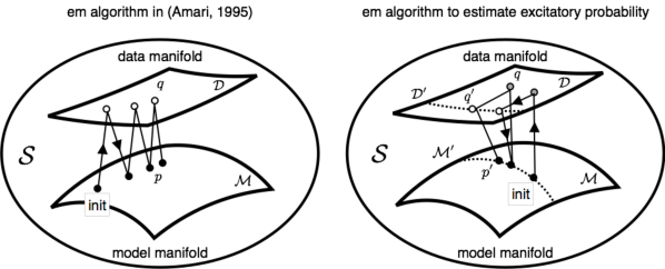
which is called the e𝑒e-projection. The em𝑒𝑚em algorithm consists of two projection steps: the e𝑒e-step and the m𝑚m-step. We note that our model manifold \mathcal{M} has the e𝑒e-flat structure and the observed data manifold 𝒟𝒟\mathcal{D} has the m𝑚m-flat structure. By iterating e𝑒e- and m𝑚m-steps alternately, the em𝑒𝑚em algorithm finds a point in esubscript𝑒\mathcal{M}\subset\mathcal{M}_{e} that is the closest to 𝒟m𝒟subscript𝑚\mathcal{D}\subset\mathcal{M}_{m}. The projection steps of the em𝑒𝑚em algorithm are shown in Fig. 3 (left).

5.3 Estimation of excitatory probability using the em𝑒𝑚em algorithm

In this study, the pseudo-connections ΛΛ\Lambda are regarded as observed random variables and the labels 𝒛𝒛\bm{z} are regarded as latent variables. Let the set of the empirical marginal distribution of ΛΛ\Lambda be a data manifold 𝒟𝒟\mathcal{D}, which is an m𝑚m-flat subspace. Any point on 𝒟𝒟\mathcal{D} represents the following distribution:

q(Λ,𝒛;𝜷)=q(Λ)q(𝒛Λ;𝜷),𝑞Λ𝒛𝜷𝑞Λ𝑞conditional𝒛Λ𝜷\displaystyle q(\Lambda,\bm{z};\bm{\beta})=q(\Lambda)q(\bm{z}\mid\Lambda;\bm{\beta}), (46)

where q(Λ)𝑞Λq(\Lambda) is the empirical distribution of ΛΛ\Lambda and 𝜷𝜷\bm{\beta} is a parameter vector with 𝒛𝒛\bm{z} similar to the parameter 𝜶𝜶\bm{\alpha}. On the other hand, a model manifold \mathcal{M} is an e𝑒e-flat subspace; hence, any point on \mathcal{M} represents the following distribution:

p(Λ,𝒛;𝜶)=p(𝒛;𝜶)p(Λ𝒛;W).𝑝Λ𝒛𝜶𝑝𝒛𝜶𝑝conditionalΛ𝒛𝑊\displaystyle p(\Lambda,\bm{z};\bm{\alpha})=p(\bm{z};\bm{\alpha})p(\Lambda\mid\bm{z};W). (47)

We assume that the distribution p(𝒛;𝜶)𝑝𝒛𝜶p(\bm{z};\bm{\alpha}) is a factorization model of a Bernoulli distribution as Eq. (38). The factorial distribution p(Λ,𝒛;𝜶)(=p(𝒛;𝜶)p(Λ𝒛;W))annotatedsuperscript𝑝Λ𝒛𝜶absentsuperscript𝑝𝒛𝜶𝑝conditionalΛ𝒛𝑊p^{\prime}(\Lambda,\bm{z};\bm{\alpha})\Bigl{(}=p^{\prime}(\bm{z};\bm{\alpha})p(\Lambda\mid\bm{z};W)\Bigr{)} consists of the e𝑒e-flat subspace superscript\mathcal{M}^{\prime}\subset\mathcal{M}. We also assume that the distribution of label 𝒛𝒛\bm{z} given observation ΛΛ\Lambda is a factorial model:

q(𝒛Λ;𝜷)=i=1Nβizi(1βi)(1zi).superscript𝑞conditional𝒛Λ𝜷superscriptsubscriptproduct𝑖1𝑁superscriptsubscript𝛽𝑖subscript𝑧𝑖superscript1subscript𝛽𝑖1subscript𝑧𝑖\displaystyle q^{\prime}(\bm{z}\mid\Lambda;\bm{\beta})=\prod_{i=1}^{N}\beta_{i}^{z_{i}}(1-\beta_{i})^{(1-z_{i})}. (48)

The distribution q(Λ,𝒛;𝜷)(=q(Λ)q(𝒛Λ;𝜷))annotatedsuperscript𝑞Λ𝒛𝜷absent𝑞Λsuperscript𝑞conditional𝒛Λ𝜷q^{\prime}(\Lambda,\bm{z};\bm{\beta})\Bigl{(}=q(\Lambda)q^{\prime}(\bm{z}\mid\Lambda;\bm{\beta})\Bigr{)} consists of the e𝑒e-flat subspace 𝒟𝒟superscript𝒟𝒟\mathcal{D}^{\prime}\subset\mathcal{D}. Therefore, we estimate the parameter 𝜶𝜶\bm{\alpha} by finding a distribution psuperscript𝑝superscriptp^{\prime}\in\mathcal{M}^{\prime} that is the closest to 𝒟superscript𝒟\mathcal{D}^{\prime}. We update two parameters, namely 𝜶𝜶\bm{\alpha} and 𝜷𝜷\bm{\beta}, as shown in Fig. 3 (right). First, the parameter 𝜷𝜷\bm{\beta} is updated by e𝑒e-projection from superscript\mathcal{M}^{\prime} to 𝒟𝒟\mathcal{D} and e𝑒e-projection from 𝒟𝒟\mathcal{D} to 𝒟superscript𝒟\mathcal{D}^{\prime}. Then, the parameter 𝜶𝜶\bm{\alpha} is updated by m𝑚m-projection from 𝒟superscript𝒟\mathcal{D}^{\prime} to superscript\mathcal{M}^{\prime}. These procedures are iterated alternately until a condition with the parameter 𝜶𝜶\bm{\alpha} is satisfied. The projection from superscript\mathcal{M}^{\prime} to 𝒟superscript𝒟\mathcal{D}^{\prime} cannot be obtained analytically; therefore, we modified the procedures from the original em𝑒𝑚em algorithm in Amari (1995). The iterative approach is described below.
Refer to caption
Figure 3: The em𝑒𝑚em algorithm in Amari (1995) is on the left and the em𝑒𝑚em algorithm to estimate excitatory probability is on the right. In the em𝑒𝑚em algorithm on the left, the projections are iterated between the dual spaces. In our em𝑒𝑚em algorithm on the right, the projections are iterated between subspaces restricted in the factorial model on the dual spaces (dashed line).

5.3.1 Projection from superscript\mathcal{M}^{\prime} to 𝒟superscript𝒟\mathcal{D}^{\prime}

The projection from the model subspace superscript\mathcal{M}^{\prime} to the data subspace 𝒟superscript𝒟\mathcal{D}^{\prime} consists of two inner steps.

Step 1. A point psuperscript𝑝superscriptp^{\prime}\in\mathcal{M}^{\prime} is projected to a point q𝒟𝑞𝒟q\in\mathcal{D} by e𝑒e-projection as

𝜷(τ+1)=missingargmin𝜷DKL[q(Λ,𝒛;𝜷),p(Λ,𝒛;𝜶(τ))].superscript𝜷𝜏1missing𝑎𝑟𝑔𝑚𝑖subscript𝑛𝜷subscript𝐷K𝐿𝑞Λ𝒛𝜷superscript𝑝Λ𝒛superscript𝜶𝜏\displaystyle\bm{\beta}^{(\tau+1)}=\mathop{\mathrm{missing}}{argmin}\limits_{\bm{\beta}}D_{\mathrm{K}L}[q(\Lambda,\bm{z};\bm{\beta}),p^{\prime}(\Lambda,\bm{z};\bm{\alpha}^{(\tau)})]. (49)

Practically, the distribution q(𝒛Λ;𝜷)𝑞conditional𝒛Λ𝜷q(\bm{z}\mid\Lambda;\bm{\beta}) is substituted by the distribution p(𝒛Λ;𝜶(τ))superscript𝑝conditional𝒛Λsuperscript𝜶𝜏p^{\prime}(\bm{z}\mid\Lambda;\bm{\alpha}^{(\tau)}) on the basis of the property of e𝑒e-projection given in Amari (1995):

q(𝒛Λ;𝜷)p(𝒛Λ;𝜶(τ)).𝑞conditional𝒛Λ𝜷superscript𝑝conditional𝒛Λsuperscript𝜶𝜏\displaystyle q(\bm{z}\mid\Lambda;\bm{\beta})\leftarrow p^{\prime}(\bm{z}\mid\Lambda;\bm{\alpha}^{(\tau)}). (50)

By Bayes’ theorem, the right-hand side of Eq. (50) is calculated by

p(𝒛Λ;𝜶(τ))=p(Λ𝒛;W)p(𝒛;𝜶(τ))𝒛p(Λ𝒛;W)p(𝒛;𝜶(τ)),superscript𝑝conditional𝒛Λsuperscript𝜶𝜏𝑝conditionalΛ𝒛𝑊superscript𝑝𝒛superscript𝜶𝜏subscript𝒛𝑝conditionalΛ𝒛𝑊superscript𝑝𝒛superscript𝜶𝜏\displaystyle p^{\prime}(\bm{z}\mid\Lambda;\bm{\alpha}^{(\tau)})=\frac{p(\Lambda\mid\bm{z};W)p^{\prime}(\bm{z};\bm{\alpha}^{(\tau)})}{\sum_{\bm{z}}p(\Lambda\mid\bm{z};W)p^{\prime}(\bm{z};\bm{\alpha}^{(\tau)})}, (51)

where p(Λ𝒛;W)𝑝conditionalΛ𝒛𝑊p(\Lambda\mid\bm{z};W) is the likelihood of observation ΛΛ\Lambda given the truncated estimator Λ^[z](=W[𝒛](IΘ)1)annotated^Λdelimited-[]𝑧absent𝑊delimited-[]𝒛superscript𝐼Θ1\hat{\Lambda}[z]\Bigl{(}=W[\bm{z}](I-\Theta)^{-1}\Bigr{)}, and we assume that the error in each pseudo-connection follows a Gaussian distribution with mean 00 and variance σe2superscriptsubscript𝜎𝑒2\sigma_{e}^{2}. Then, the distribution p(Λ𝒛;W)𝑝conditionalΛ𝒛𝑊p(\Lambda\mid\bm{z};W) is calculated by

p(Λ𝒛;W)𝑝conditionalΛ𝒛𝑊\displaystyle p(\Lambda\mid\bm{z};W) =i,j[12πσe2exp{(λijλ^ij)22σe2}]\displaystyle=\prod_{i,j}\Biggr{[}\frac{1}{\sqrt{2\pi\sigma_{e}^{2}}}\exp\Bigl{\{}-\frac{(\lambda_{ij}-\hat{\lambda}_{ij})^{2}}{2\sigma_{e}^{2}}\Bigr{\}}\Biggl{]}
=i,j,λij>0[12πσe2exp{(λijλ^ij)22σe2}]\displaystyle=\prod_{i,j,\lambda_{ij}>0}\Biggr{[}\frac{1}{\sqrt{2\pi\sigma_{e}^{2}}}\exp\Bigl{\{}-\frac{(\lambda_{ij}-\hat{\lambda}_{ij})^{2}}{2\sigma_{e}^{2}}\Bigr{\}}\Biggl{]}
×i,j,λij<0[12πσe2exp{(λijλ^ij)22σe2}]\displaystyle\qquad\qquad\times\prod_{i,j,\lambda_{ij}<0}\Biggr{[}\frac{1}{\sqrt{2\pi\sigma_{e}^{2}}}\exp\Bigl{\{}-\frac{(\lambda_{ij}-\hat{\lambda}_{ij})^{2}}{2\sigma_{e}^{2}}\Bigr{\}}\Biggl{]}
i,j,λij>0[12πσe2exp{(λijλ^ij)22σe2}].\displaystyle\simeq\prod_{i,j,\lambda_{ij}>0}\Biggr{[}\frac{1}{\sqrt{2\pi\sigma_{e}^{2}}}\exp\Bigl{\{}-\frac{(\lambda_{ij}-\hat{\lambda}_{ij})^{2}}{2\sigma_{e}^{2}}\Bigr{\}}\Biggl{]}. (52)

In the above expansion, we assume that σe0much-greater-thansubscript𝜎𝑒0\sigma_{e}\gg 0 if λij<0subscript𝜆𝑖𝑗0\lambda_{ij}<0.

Step 2. A point q𝒟𝑞𝒟q\in\mathcal{D} is projected to a point q𝒟superscript𝑞superscript𝒟q^{\prime}\in\mathcal{D}^{\prime} by e𝑒e-projection as

𝜷(τ+1)=missingargmin𝜷DKL[q(Λ,𝒛;𝜶(τ)),q(Λ,𝒛;𝜷)].superscript𝜷𝜏1missing𝑎𝑟𝑔𝑚𝑖subscript𝑛𝜷subscript𝐷KLsuperscript𝑞Λ𝒛superscript𝜶𝜏𝑞Λ𝒛𝜷\displaystyle\bm{\beta}^{(\tau+1)}=\mathop{\mathrm{missing}}{argmin}\limits_{\bm{\beta}}D_{\mathrm{KL}}[q^{\prime}(\Lambda,\bm{z};\bm{\alpha}^{(\tau)}),q(\Lambda,\bm{z};\bm{\beta})]. (53)

Hence, the parameter 𝜷𝜷\bm{\beta} is updated by

βi(τ+1)superscriptsubscript𝛽𝑖𝜏1\displaystyle\beta_{i}^{(\tau+1)} 11+exp{A(τ)},absentcontinued-fraction11superscript𝐴𝜏\displaystyle\leftarrow\cfrac{1}{1+\exp{\bigl{\{}-A^{(\tau)}\bigr{\}}}}, (54)
A(τ)superscript𝐴𝜏\displaystyle A^{(\tau)} =𝒛iq(𝒛iΛ;β)logp(𝒛iΛ,zi=1;𝜶(τ))p(𝒛iΛ,zi=0;𝜶(τ)),absentsubscriptsubscript𝒛𝑖superscript𝑞conditionalsubscript𝒛𝑖Λ𝛽continued-fractionsuperscript𝑝conditionalsubscript𝒛𝑖Λsubscript𝑧𝑖1superscript𝜶𝜏superscript𝑝conditionalsubscript𝒛𝑖Λsubscript𝑧𝑖0superscript𝜶𝜏\displaystyle=\sum_{\bm{z}_{-i}}q^{\prime}(\bm{z}_{-i}\mid\Lambda;\beta)\log{\cfrac{p^{\prime}(\bm{z}_{-i}\mid\Lambda,z_{i}=1;\bm{\alpha}^{(\tau)})}{p^{\prime}(\bm{z}_{-i}\mid\Lambda,z_{i}=0;\bm{\alpha}^{(\tau)})}}, (55)

where 𝒛i=(z1,,zi1,zi+1,,zN)subscript𝒛𝑖subscript𝑧1subscript𝑧𝑖1subscript𝑧𝑖1subscript𝑧𝑁\bm{z}_{-i}=(z_{1},\cdots,z_{i-1},z_{i+1},\cdots,z_{N}) and q(𝒛iΛ;β)superscript𝑞conditionalsubscript𝒛𝑖Λ𝛽q^{\prime}(\bm{z}_{-i}\mid\Lambda;\beta) is given by q(𝒛iΛ;β)=jiβjzj(1βj)1zjsuperscript𝑞conditionalsubscript𝒛𝑖Λ𝛽subscriptproduct𝑗𝑖superscriptsubscript𝛽𝑗subscript𝑧𝑗superscript1subscript𝛽𝑗1subscript𝑧𝑗q^{\prime}(\bm{z}_{-i}\mid\Lambda;\beta)=\prod_{j\neq i}\beta_{j}^{z_{j}}(1-\beta_{j})^{1-z_{j}}. In this step, q𝒟superscript𝑞superscript𝒟q^{\prime}\in\mathcal{D}^{\prime}, the closest point to q𝒟𝑞𝒟q\in\mathcal{D}, needs to be obtained by projection. Both e𝑒e-projection and m𝑚m-projection can be used in this step because the KL divergence between q𝒟superscript𝑞superscript𝒟q^{\prime}\in\mathcal{D}^{\prime} and q𝒟𝑞𝒟q\in\mathcal{D} is small. In this study, e𝑒e-projection is adopted. The subspace 𝒟superscript𝒟\mathcal{D}^{\prime} is e𝑒e-flat; hence, the e𝑒e-projection to 𝒟superscript𝒟\mathcal{D}^{\prime} is not uniquely determined in general. However, it is experimentally confirmed that there is no significant difference between the estimations of the excitatory probability 𝜶𝜶\bm{\alpha} by e𝑒e-projection and m𝑚m-projection in this step.

5.3.2 Projection from 𝒟superscript𝒟\mathcal{D}^{\prime} to superscript\mathcal{M}^{\prime}

The m𝑚m-projection of the distribution q𝒟superscript𝑞superscript𝒟q^{\prime}\in\mathcal{D}^{\prime} to superscript\mathcal{M}^{\prime} gives the distribution psuperscript𝑝p^{\prime}, i.e.,

𝜶(τ+1)=missingargmin𝜶DKL[q(Λ,𝒛;𝜷(τ)),p(Λ,𝒛;𝜶)].superscript𝜶𝜏1missing𝑎𝑟𝑔𝑚𝑖subscript𝑛𝜶subscript𝐷KLsuperscript𝑞Λ𝒛superscript𝜷𝜏𝑝Λ𝒛𝜶\displaystyle\bm{\alpha}^{(\tau+1)}=\mathop{\mathrm{missing}}{argmin}\limits_{\bm{\alpha}}D_{\mathrm{KL}}[q^{\prime}(\Lambda,\bm{z};\bm{\beta}^{(\tau)}),p(\Lambda,\bm{z};\bm{\alpha})]. (56)

Therefore, parameter 𝜶𝜶\bm{\alpha} is updated by

αi(τ+1)𝒛ziq(ziΛ;𝜷(τ)).superscriptsubscript𝛼𝑖𝜏1subscript𝒛subscript𝑧𝑖superscript𝑞conditionalsubscript𝑧𝑖Λsuperscript𝜷𝜏\displaystyle\alpha_{i}^{(\tau+1)}\leftarrow\sum_{\bm{z}}z_{i}q^{\prime}(z_{i}\mid\Lambda;\bm{\beta}^{(\tau)}). (57)

The derivation of the em𝑒𝑚em algorithm to estimate parameter 𝜶𝜶\bm{\alpha} is given in Appendix B.

These two steps are iterated until parameter 𝜶𝜶\bm{\alpha} converges. The proposed algorithm is summarized in Algorithm 3. If the estimated value of αisubscript𝛼𝑖\alpha_{i} is equal to 111, neuron i𝑖i is classified as excitatory; otherwise, neuron i𝑖i is classified as inhibitory.

Algorithm 3 em𝑒𝑚em algorithm to estimate excitatory probability
1:Inputs: ΛΛ\Lambda, C^^𝐶\hat{C}
2:Initialization: αi(1)12,i=1,2,,Nformulae-sequencesuperscriptsubscript𝛼𝑖112𝑖12𝑁{\alpha}_{i}^{(1)}\leftarrow\frac{1}{2},\;\;i=1,2,\cdots,N
3:while until convergence do
4:     for all 𝒛{0,1}N𝒛superscript01𝑁\bm{z}\in\{0,1\}^{N} do
5:         W(𝒛)estimateW_label(Λ,C¯,𝒛)𝑊𝒛estimateW_labelΛ¯𝐶𝒛W(\bm{z})\leftarrow\textsc{estimateW\_label}(\Lambda,\bar{C},\bm{z})
6:         Λ^=W[𝒛](IΘ)1^Λ𝑊delimited-[]𝒛superscript𝐼Θ1\hat{\Lambda}=W[\bm{z}](I-\Theta)^{-1}
7:         p(Λ𝒛)=i,j[12πσe2exp{(λijλ^ij)22σe2}]p(\Lambda\mid\bm{z})=\prod_{i,j}\Bigr{[}\frac{1}{\sqrt{2\pi\sigma_{e}^{2}}}\exp\Bigl{\{}-\frac{(\lambda_{ij}-\hat{\lambda}_{ij})^{2}}{2\sigma_{e}^{2}}\Bigr{\}}\Bigl{]} \triangleright Eq. (52)
8:     end for
9:     q(𝒛Λ;𝜶(τ))p(Λ𝒛)p(𝒛;𝜶(τ))𝒛p(Λ𝒛)p(𝒛;𝜶(τ))𝑞conditional𝒛Λsuperscript𝜶𝜏𝑝conditionalΛ𝒛𝑝𝒛superscript𝜶𝜏subscript𝒛𝑝conditionalΛ𝒛𝑝𝒛superscript𝜶𝜏q(\bm{z}\mid\Lambda;\bm{\alpha}^{(\tau)})\leftarrow\frac{p(\Lambda\mid\bm{z})p(\bm{z};\bm{\alpha}^{(\tau)})}{\sum_{\bm{z}}p(\Lambda\mid\bm{z})p(\bm{z};\bm{\alpha}^{(\tau)})} \triangleright Eq. (50)
10:     A(τ)=𝒛iq(𝒛iΛ;β)logp(𝒛iΛ,zi=1;𝜶(τ))p(𝒛iΛ,zi=0;𝜶(τ))superscript𝐴𝜏subscriptsubscript𝒛𝑖superscript𝑞conditionalsubscript𝒛𝑖Λ𝛽𝑝conditionalsubscript𝒛𝑖Λsubscript𝑧𝑖1superscript𝜶𝜏𝑝conditionalsubscript𝒛𝑖Λsubscript𝑧𝑖0superscript𝜶𝜏A^{(\tau)}=\sum_{\bm{z}_{-i}}q^{\prime}(\bm{z}_{-i}\mid\Lambda;\beta)\log{\frac{p(\bm{z}_{-i}\mid\Lambda,z_{i}=1;\bm{\alpha}^{(\tau)})}{p(\bm{z}_{-i}\mid\Lambda,z_{i}=0;\bm{\alpha}^{(\tau)})}} \triangleright Eq. (55)
11:     βi(τ+1)11+exp{A(τ)}superscriptsubscript𝛽𝑖𝜏111superscript𝐴𝜏\beta_{i}^{(\tau+1)}\leftarrow\frac{1}{1+\exp{\bigl{\{}-A^{(\tau)}\bigr{\}}}}
12:     αi(τ+1)𝒛ziq(ziΛ;𝜷(τ+1))superscriptsubscript𝛼𝑖𝜏1subscript𝒛subscript𝑧𝑖superscript𝑞conditionalsubscript𝑧𝑖Λsuperscript𝜷𝜏1\alpha_{i}^{(\tau+1)}\leftarrow\sum_{\bm{z}}z_{i}q^{\prime}(z_{i}\mid\Lambda;\bm{\beta}^{(\tau+1)}) \triangleright Eq. (57)
13:end while
14:Output: 𝜶𝜶\bm{\alpha}

5.3.3 Approximated algorithm by Gibbs sampling

Algorithm 3 is computationally expensive because of the combinatorial explosion. The variables 𝒛{1,0}N𝒛superscript10𝑁\bm{z}\in\{1,0\}^{N} have 2Nsuperscript2𝑁2^{N} combinations. The computational costs of Eq. (50), Eq. (55), and Eq. (57) rapidly increase with the number of neurons N𝑁N. To overcome this difficulty, we approximate Eq. (55) by Gibbs sampling. Gibbs sampling is a Markov chain Monte Carlo (MCMC) sampling technique that is used for computing the statistics of a target distribution approximately when direct sampling from the distribution is difficult. Here, the target distribution is qsuperscript𝑞q^{\prime} in Eq. (55). Suppose that we generate K𝐾K samples from distribution qsuperscript𝑞q^{\prime}. The k𝑘k-th sample zi(k)superscriptsubscript𝑧𝑖𝑘z_{i}^{(k)} of zisubscript𝑧𝑖z_{i} is sampled by

zi(k+1)q(ziz1(k),zi1(k),zi+1(k),,zN(k),Λ;𝜶).similar-tosuperscriptsubscript𝑧𝑖𝑘1superscript𝑞conditionalsubscript𝑧𝑖superscriptsubscript𝑧1𝑘superscriptsubscript𝑧𝑖1𝑘superscriptsubscript𝑧𝑖1𝑘superscriptsubscript𝑧𝑁𝑘Λ𝜶\displaystyle z_{i}^{(k+1)}\sim q^{\prime}(z_{i}\mid z_{1}^{(k)},\cdots z_{i-1}^{(k)},z_{i+1}^{(k)},\cdots,z_{N}^{(k)},\Lambda;\bm{\alpha}). (58)

From Eq. (50), Eq. (58) is given by

zi(k+1)p1p1+p0,similar-tosuperscriptsubscript𝑧𝑖𝑘1subscript𝑝1subscript𝑝1subscript𝑝0\displaystyle z_{i}^{(k+1)}\sim\frac{p_{1}}{p_{1}+p_{0}}, (59)

where p1subscript𝑝1p_{1} and p0subscript𝑝0p_{0} are calculated by

p1subscript𝑝1\displaystyle p_{1} =p(Λzi=1,𝒛i(k);W)p(zi=1,𝒛i(k);𝜶(τ)),absent𝑝conditionalΛsubscript𝑧𝑖1superscriptsubscript𝒛𝑖𝑘𝑊𝑝subscript𝑧𝑖1superscriptsubscript𝒛𝑖𝑘superscript𝜶𝜏\displaystyle=p(\Lambda\!\mid\!z_{i}\!=\!1,\bm{z}_{-i}^{(k)};W)p(z_{i}\!=\!1,\bm{z}_{-i}^{(k)};\bm{\alpha}^{(\tau)}), (60)
p0subscript𝑝0\displaystyle p_{0} =p(Λzi=0,𝒛i(k);W)p(zi=0,𝒛i(k);𝜶(τ)),absent𝑝conditionalΛsubscript𝑧𝑖0superscriptsubscript𝒛𝑖𝑘𝑊𝑝subscript𝑧𝑖0superscriptsubscript𝒛𝑖𝑘superscript𝜶𝜏\displaystyle=p(\Lambda\!\mid\!z_{i}\!=\!0,\bm{z}_{-i}^{(k)};W)p(z_{i}\!=\!0,\bm{z}_{-i}^{(k)};\bm{\alpha}^{(\tau)}), (61)

where 𝒛i(k)={z1(k),zi1(k),zi+1(k),,zN(k)}superscriptsubscript𝒛𝑖𝑘superscriptsubscript𝑧1𝑘superscriptsubscript𝑧𝑖1𝑘superscriptsubscript𝑧𝑖1𝑘superscriptsubscript𝑧𝑁𝑘\bm{z}_{-i}^{(k)}=\{z_{1}^{(k)},\cdots z_{i-1}^{(k)},z_{i+1}^{(k)},\cdots,z_{N}^{(k)}\}. By using sampled {𝒛(k)}k=1,,Ksubscriptsuperscript𝒛𝑘𝑘1𝐾\{\bm{z}^{(k)}\}_{k=1,\cdots,K}, we approximate Eq. (50) and Eq. (55) by

𝜷i(τ+1)1Kk=1Kq(𝒛i(k)Λ;β)logp(𝒛i(k)Λ,zi=1;𝜶(τ))p(𝒛i(k)Λ,zi=0;𝜶(τ)).superscriptsubscript𝜷𝑖𝜏11𝐾superscriptsubscript𝑘1𝐾superscript𝑞conditionalsuperscriptsubscript𝒛𝑖𝑘Λ𝛽continued-fraction𝑝conditionalsuperscriptsubscript𝒛𝑖𝑘Λsubscript𝑧𝑖1superscript𝜶𝜏𝑝conditionalsuperscriptsubscript𝒛𝑖𝑘Λsubscript𝑧𝑖0superscript𝜶𝜏\displaystyle\bm{\beta}_{i}^{(\tau+1)}\leftarrow\frac{1}{K}\sum_{k=1}^{K}q^{\prime}(\bm{z}_{-i}^{(k)}\mid\Lambda;\beta)\log{\cfrac{p(\bm{z}_{-i}^{(k)}\mid\Lambda,z_{i}=1;\bm{\alpha}^{(\tau)})}{p(\bm{z}_{-i}^{(k)}\mid\Lambda,z_{i}=0;\bm{\alpha}^{(\tau)})}}. (62)

Eq. (57) is calculated by sampling 𝒛𝒛\bm{z} randomly. We let the estimator of 𝜶𝜶\bm{\alpha} be the mean of M𝜶subscript𝑀𝜶M_{\bm{\alpha}} estimates of 𝜶𝜶\bm{\alpha} by using the em𝑒𝑚em algorithm:

α¯i=1M𝜶m=1M𝜶αim,subscript¯𝛼𝑖1subscript𝑀𝜶superscriptsubscript𝑚1subscript𝑀𝜶superscriptsubscript𝛼𝑖𝑚\displaystyle\bar{\alpha}_{i}=\frac{1}{M_{\bm{\alpha}}}\sum_{m=1}^{M_{\bm{\alpha}}}\alpha_{i}^{m}, (63)

where αimsuperscriptsubscript𝛼𝑖𝑚\alpha_{i}^{m} is a parameter of the m𝑚m-th label estimation. If the value of α¯isubscript¯𝛼𝑖\bar{\alpha}_{i} is equal to 111, neuron i𝑖i is classified as excitatory; otherwise, neuron i𝑖i is classified as inhibitory.

6 Numerical simulations

In this section, the proposed methods are verified using synthesized data.

6.1 Spiking model

We generated synthetic data using a simple spiking model proposed by Izhikevich (2003). This model is known to be able to simulate various types of cortical neuron behaviors. Following Izhikevich (2003), we used regular spiking cells to model excitatory neurons and fast spiking cells to model inhibitory neurons. The four parameters that specify a neuron’s behavior are summarized in Table 1. The variables resubscript𝑟𝑒r_{e} and risubscript𝑟𝑖r_{i} are random variables from a uniform distribution with the interval [0,1]01[0,1].

Table 1: Parameters that specify a neuron’s behavior in Izhikevich (2003)
a𝑎a b𝑏b c𝑐c d𝑑d
excitatory 0.020.020.02 0.20.20.2 65+15re26515superscriptsubscript𝑟𝑒2-65+15r_{e}^{2} 86re286superscriptsubscript𝑟𝑒28-6r_{e}^{2}
inhibitory 0.02+0.08ri0.020.08subscript𝑟𝑖0.02+0.08r_{i} 0.250.05ri0.250.05subscript𝑟𝑖0.25-0.05r_{i} 6565-65 222

6.2 Synthetic data

6.2.1 Network of 100 neurons

To investigate the performance of the proposed method in a simple setting, we constructed a network of 100 neurons (NA=100subscript𝑁𝐴100N_{A}=100). On the basis of neuroscience evidence, 808080 neurons were excitatory and 202020 neurons were inhibitory, and the number of connections from one neuron to others was set to at most 101010 (corresponding to a 10%percent1010\% connection ratio). Their excitatory and inhibitory connect weights follow uniform distributions [0,10]010[0,10] and [10,0]100[-10,0], respectively. To investigate the performance for partial observations, we randomly sampled N=33𝑁33N=33 neurons and constructed a connection matrix WN×Nsuperscript𝑊superscript𝑁𝑁W^{*}\in\mathbb{R}^{N\times N} from NA=100subscript𝑁𝐴100N_{A}=100 neurons. The number of unobserved neurons was set to be twice as high as that of observed ones. A network activity was simulated for 1 h with a temporal resolution of 1 ms.

6.2.2 Network of 10,000 neurons

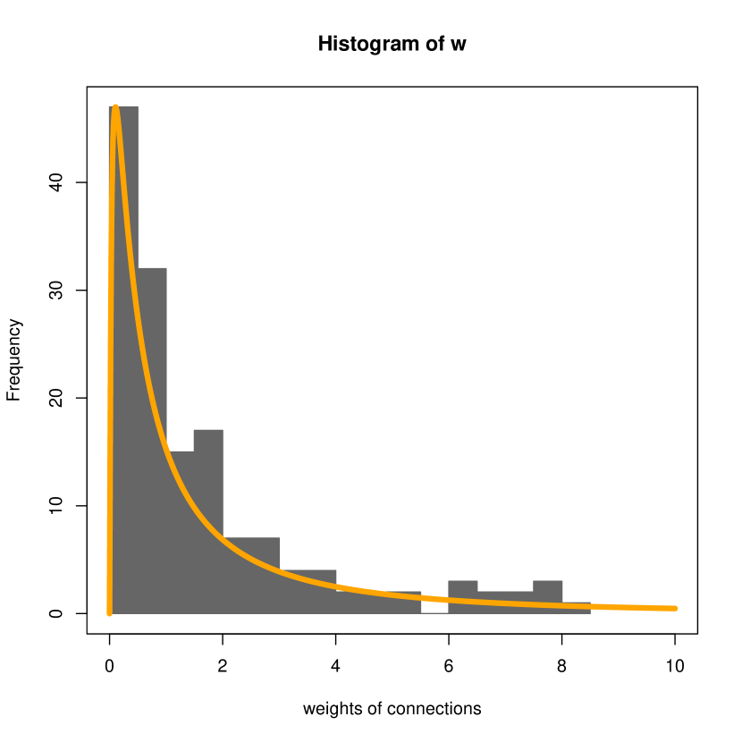
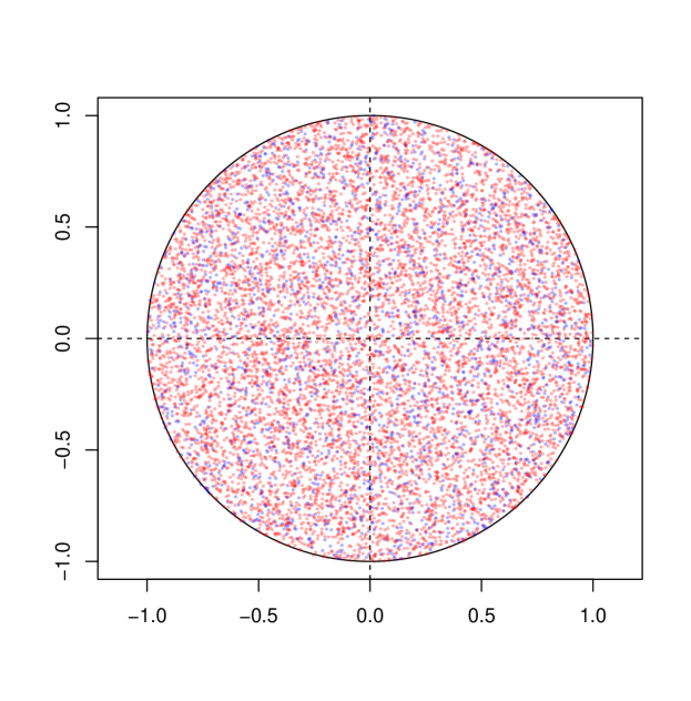
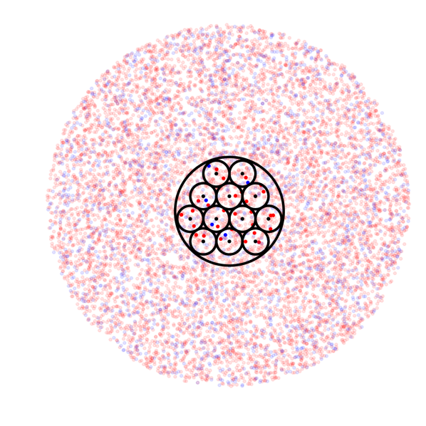
To evaluate how the proposed method works under a realistic condition, we also constructed a network of 10,0001000010,000 neurons (NA=10,000subscript𝑁𝐴10000N_{A}=10,000) in which 8,00080008,000 neurons are excitatory and 2,00020002,000 neurons are inhibitory. The neurons are scattered on a 2-D plane and the connection weights follow a log-normal distribution (Song et al., 2005), as shown in Fig. 4. The number of connections of each neuron is set to 150.
Refer to caption
Refer to caption
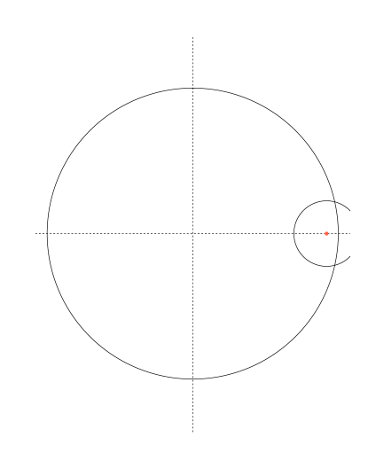
Figure 4: Schematic illustration of 10,0001000010,000-neuron simulation and distribution of the connection weights. Left: Positions of 10,000 neurons and sampled neurons and 12 tetrodes. The light red and blue dots represent excitatory and inhibitory neurons, respectively. The 12 small black circles represent the recording range of the tetrodes. The dark red and blue dots represent the sampled neurons. Right: Histogram of connection weights. The orange line represents the log-normal distribution (mean 00 and variance 1.52superscript1.521.5^{2}) from which the connection weights were sampled.

The details of how the network was generated are given in Appendix C. To investigate the performance for partial observation, we randomly sampled N=33𝑁33N=33 neurons out of NA=10,000subscript𝑁𝐴10000N_{A}=10,000 neurons and constructed a connection matrix WN×Nsuperscript𝑊superscript𝑁𝑁W^{*}\in\mathbb{R}^{N\times N}. In multi-electrode recording, such as hyper-drive recording (Gothard et al., 1996), 12 tetrodes (TTs) are arranged as shown in Fig. 4. The small inner circles represent the recording range of each TT and the large outer circle represents the entire hyper-drive recording range, which is approximately 1 mm in diameter. A network activity was simulated for 1 h with a temporal resolution of 1 ms.

6.3 Comparative methods

We compared the proposed method with two commonly used methods, namely the cross-correlation function and binary logistic regression.

6.3.1 Cross-correlation function

The cross-correlation function is often used to estimate neural interactions (Wilson and McNaughton, 1994; Barthó et al., 2004). A cross-correlation function between neurons i𝑖i and j𝑗j for a time lag s𝑠s\in\mathbb{N}, CCij(s)subscriptCC𝑖𝑗𝑠\mathrm{CC}_{ij}(s) is defined as

CCij(s)=t=1TXi(t)Xj(t+s).subscriptCC𝑖𝑗𝑠superscriptsubscript𝑡1𝑇subscript𝑋𝑖𝑡subscript𝑋𝑗𝑡𝑠\displaystyle\mathrm{CC}_{ij}(s)=\sum_{t=1}^{T}X_{i}(t)X_{j}(t+s). (64)

Connection weight wijsubscript𝑤𝑖𝑗w_{ij} from neuron j𝑗j to neuron i𝑖i is estimated by

wij=maxsCCij(s)s=1Δ|CCij(s)|,subscript𝑤𝑖𝑗subscript𝑠continued-fractionsubscriptCC𝑖𝑗𝑠superscriptsubscript𝑠1ΔsubscriptCC𝑖𝑗𝑠\displaystyle w_{ij}=\max_{s}{\cfrac{\mathrm{CC}_{ij}(s)}{\sum_{s=1}^{\Delta}\left|\mathrm{CC}_{ij}(s)\right|}}, (65)

where the value ΔΔ\Delta is the maximum time lag, which is the same as the time window ΔΔ\Delta used in the proposed method.

6.3.2 Binary logistic regression with L1subscript𝐿1L_{1} regularization

Binary logistic regression is a standard statistical method to estimate the probability that a response variable is 1 and to assess an unobserved input. To estimate the connections to neuron i𝑖i, let a variable set

𝑿i[tΔ]={X1[tΔ],,Xi1[tΔ],Xi+1[tΔ],,XN[tΔ]}subscript𝑿𝑖delimited-[]subscript𝑡Δsubscript𝑋1delimited-[]subscript𝑡Δsubscript𝑋𝑖1delimited-[]subscript𝑡Δsubscript𝑋𝑖1delimited-[]subscript𝑡Δsubscript𝑋𝑁delimited-[]subscript𝑡Δ\displaystyle\bm{X}_{-i}[t_{\Delta}]=\{X_{1}[t_{\Delta}],\cdots,X_{i-1}[t_{\Delta}],X_{i+1}[t_{\Delta}],\cdots,X_{N}[t_{\Delta}]\} (66)

consist of explanatory variables and let a variable Xi(t)subscript𝑋𝑖𝑡X_{i}(t) be a response variable. The estimated probability pisubscript𝑝𝑖p_{i} is given by

pi(t)=Pr(Xi(t)=1𝑿i[tΔ])=11+exp(bi𝒘iT𝑿i[tΔ]),subscript𝑝𝑖𝑡Prsubscript𝑋𝑖𝑡conditional1subscript𝑿𝑖delimited-[]subscript𝑡Δ11subscript𝑏𝑖superscriptsubscript𝒘𝑖Tsubscript𝑿𝑖delimited-[]subscript𝑡Δ\displaystyle p_{i}(t)=\mathrm{Pr}(X_{i}(t)=1\mid\bm{X}_{-i}[t_{\Delta}])=\frac{1}{1+\exp{\Bigl{(}-b_{i}-\bm{w}_{i}^{\mathrm{T}}\bm{X}_{-i}[t_{\Delta}]\Bigr{)}}}, (67)

where bisubscript𝑏𝑖b_{i} is a parameter representing an unobserved input and 𝒘iN1subscript𝒘𝑖superscript𝑁1\bm{w}_{i}\in\mathbb{R}^{N-1} is a coefficient. The j𝑗j-th element wijsubscript𝑤𝑖𝑗w_{ij} of 𝒘isubscript𝒘𝑖\bm{w}_{i} represents the connection weight from neuron j𝑗j to neuron i𝑖i. The parameters bisubscript𝑏𝑖b_{i} and 𝒘isubscript𝒘𝑖\bm{w}_{i} are estimated by maximizing the log likelihood function with L1subscript𝐿1L_{1} regularization:

bi,𝒘i=missingargminbi,𝒘i{(bi,𝒘i)+λj=1N1|wij|},subscript𝑏𝑖subscript𝒘𝑖missing𝑎𝑟𝑔𝑚𝑖subscript𝑛subscript𝑏𝑖subscript𝒘𝑖subscript𝑏𝑖subscript𝒘𝑖𝜆superscriptsubscript𝑗1𝑁1subscript𝑤𝑖𝑗\displaystyle b_{i},\bm{w}_{i}=\mathop{\mathrm{missing}}{argmin}\limits_{b_{i},\bm{w}_{i}}\Bigl{\{}-\ell(b_{i},\bm{w}_{i})+\lambda\sum_{j=1}^{N-1}|w_{ij}|\Bigr{\}}, (68)

where λ𝜆\lambda is a regularization parameter, which is determined by 10-fold cross-validation in this study. The log-likelihood function (bi,𝒘i)subscript𝑏𝑖subscript𝒘𝑖\ell(b_{i},\bm{w}_{i}) is given by

(bi,𝒘i)=t=ΔT{logpi(t)+(1Xi(t))(bi𝒘iT𝑿i[tΔ])}.subscript𝑏𝑖subscript𝒘𝑖superscriptsubscript𝑡Δ𝑇subscript𝑝𝑖𝑡1subscript𝑋𝑖𝑡subscript𝑏𝑖superscriptsubscript𝒘𝑖Tsubscript𝑿𝑖delimited-[]subscript𝑡Δ\displaystyle\ell(b_{i},\bm{w}_{i})=\sum_{t=\Delta}^{T}\Bigl{\{}\log{p_{i}(t)}+\bigl{(}1-X_{i}(t)\bigr{)}\Bigl{(}-b_{i}-\bm{w}_{i}^{\mathrm{T}}\bm{X}_{-i}[t_{\Delta}]\Bigr{)}\Bigr{\}}. (69)

6.4 Evaluation of estimated W𝑊W

The performance of the proposed method was assessed by comparing the estimated graph W𝑊W and the true graph Wsuperscript𝑊W^{*}. We used two evaluation indices, namely sensitivity and Kendall rank correlation coefficient.

6.4.1 Sensitivity

The true positive (TP) is defined by the number of connections that satisfy both wij0subscript𝑤𝑖𝑗0w_{ij}\neq 0 and wij0superscriptsubscript𝑤𝑖𝑗0w_{ij}^{*}\neq 0, and the false negative (FN) is defined by the number of connections that satisfy wij=0subscript𝑤𝑖𝑗0w_{ij}=0 and wij0superscriptsubscript𝑤𝑖𝑗0w_{ij}^{*}\neq 0. The sensitivity is calculated by

Senstivity=TPTP+FN[0,1].SenstivityTPTPFN01\displaystyle\mathrm{Senstivity}=\frac{{\rm TP}}{{\rm TP}+{\rm FN}}\in[0,1]. (70)

The sensitivity gives the rate of correctly estimated connections.

6.4.2 Kendall rank correlation coefficient

If Wsuperscript𝑊W^{*} and W𝑊W are vectorized as 𝒘N2superscript𝒘superscriptsuperscript𝑁2{\bm{w}}^{*}\in\mathbb{R}^{N^{2}} and 𝒘N2𝒘superscriptsuperscript𝑁2{\bm{w}}\in\mathbb{R}^{N^{2}}, wisubscriptsuperscript𝑤𝑖w^{*}_{i} and wisubscript𝑤𝑖w_{i} are the i𝑖i-th elements of 𝒘superscript𝒘{\bm{w}}^{*} and 𝒘𝒘\bm{w}, respectively. The Kendall rank correlation coefficient τKsubscript𝜏K\tau_{\mathrm{K}} is defined by

τKsubscript𝜏K\displaystyle\tau_{\mathrm{K}} =i,jNQijP2N,absentsuperscriptsubscript𝑖𝑗𝑁subscript𝑄𝑖𝑗subscriptsubscript𝑃2𝑁\displaystyle=\frac{\sum_{i,j}^{N}Q_{ij}}{{}_{N}P_{2}}, (71)
Qijsubscript𝑄𝑖𝑗\displaystyle Q_{ij} =sgn(wiwi)sgn(wjwj).absentsgnsubscriptsuperscript𝑤𝑖subscript𝑤𝑖sgnsubscriptsuperscript𝑤𝑗subscript𝑤𝑗\displaystyle=\mathrm{sgn}(w^{*}_{i}-w_{i})\cdot\mathrm{sgn}(w^{*}_{j}-w_{j}). (72)

τK=1subscript𝜏K1\tau_{\mathrm{K}}=1 is obtained when the method estimates the rank of connections exactly. Note that the Kendall rank correlation coefficient requires W𝑊W and Wsuperscript𝑊W^{*} to have the same number of connections. Therefore, we calculate the Kendall rank correlation coefficient by choosing the connections included in both W𝑊W and in Wsuperscript𝑊W^{*}.

6.5 Results

6.5.1 Network of 100 neurons

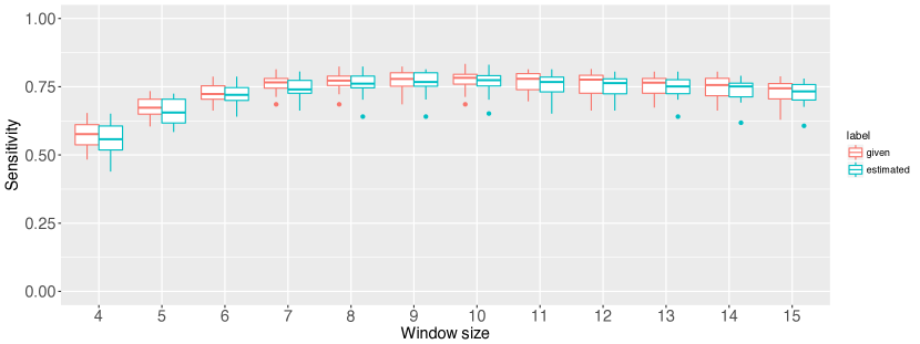
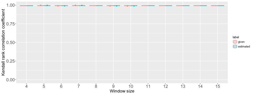
We generated five different networks. From each of them, 20 different graphs consisting of 33 neurons were sampled. Starting from the window size Δ=4Δ4\Delta=4, simulations were conducted until the sensitivity did not change significantly. We examined 12 different time window sizes: Δ=4,5,6,,14,15Δ4561415\Delta=4,5,6,\cdots,14,15[ms]. To simplify the evaluation of the results, we removed weak connections from W𝑊W such that the number of connections in W𝑊W was the same as that in Wsuperscript𝑊W^{*}. Fig. 5 and Fig. 6 show the results of sensitivity and Kendall rank correlation coefficient analyses, respectively. The horizontal axis represents the size of the time window, Δ=4,5,6,,14,15Δ4561415\Delta=4,5,6,\cdots,14,15. For each value of ΔΔ\Delta, there are two box plots. The ones on the left are the results obtained from Algorithm 2 given excitatory-inhibitory labels 𝒛𝒛\bm{z}. The ones on the right are the results obtained from Algorithm 2 and the estimated excitatory-inhibitory labels 𝒛𝒛\bm{z}. In Fig. 5, we see relatively high sensitivity, which peaks at around 0.760.760.76 around Δ=10Δ10\Delta=10[ms]. The results show that the proposed method estimated 76%percent7676\% of Wsuperscript𝑊W^{*} connections correctly when spike interactions over 10similar-toabsent10\sim 10[ms] were considered. When Δ>10Δ10\Delta>10[ms], i.e., in the case of a long time window, more propagations via multiple neurons were detected and the sensitivity was reduced. In Fig. 6, the value of the Kendall rank correlation coefficient is nearly 1, suggesting that the proposed method detected the order of strong connections correctly. Together with Fig. 5, we confirmed that our method detected the major connections in the network of 100 neurons successfully, even if only part of the neurons was observed. Importantly, the performance did not decline significantly when the label 𝒛𝒛\bm{z} was also estimated from the data (shown in blue in Fig. 5 and Fig. 6). This is a particularly favorable property because the neuron type, whether excitatory or inhibitory, may not be easily obtained in real experiments.
Refer to caption
Figure 5: Sensitivity measures to evaluate the performance of the proposed method in graphs composed of 33 neurons sampled from a network of 100 neurons. The horizontal axis represents the size of the time window: Δ=4,5,6,,14,15Δ4561415\Delta=4,5,6,\cdots,14,15. For each ΔΔ\Delta, the left box plot represents the sensitivity estimated by Algorithm 2 given excitatory-inhibitory labels 𝒛𝒛\bm{z} and the right box plot represents the sensitivity estimated by Algorithm 2 and the estimated label 𝒛𝒛\bm{z}.
Refer to caption
Figure 6: Kendall rank correlation coefficient measures to evaluate the performance of the proposed method in graphs composed of 33 neurons sampled from a network of 100 neurons. The horizontal axis represents the size of the time window: Δ=4,5,6,,14,15Δ4561415\Delta=4,5,6,\cdots,14,15. For each ΔΔ\Delta, the left box plot represents the Kendall rank correlation coefficient estimated by Algorithm 2 given excitatory-inhibitory label 𝒛𝒛\bm{z} and the right box plot represents the Kendall rank correlation coefficient estimated by Algorithm 2 and the estimated excitatory-inhibitory label 𝒛𝒛\bm{z}.

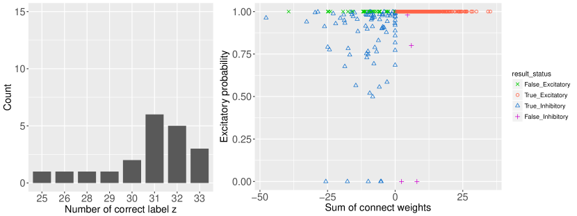
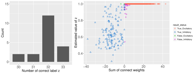
To investigate how the proposed method with the estimated label 𝒛𝒛\bm{z} achieved the good performance, we show how the label 𝒛𝒛\bm{z} was estimated in the time window Δ=10Δ10\Delta=10[ms] in Fig. 7. On the left, the number of correctly estimated labels is plotted. In Fig. 7, we see that the number of incorrectly estimated neurons is at most 3 among the 33 sampled neurons. On the right, the estimated values of label 𝒛𝒛\bm{z} are plotted as a function of the sum of out-going connection weights of each neuron. The results are summarized by four different symbols:  correctly estimated excitatory neurons (\circ), incorrectly estimated excitatory neurons (++), correctly estimated inhibitory neurons (\bigtriangleup), and incorrectly estimated inhibitory neurons (×\times). We see that incorrectly estimated neurons have weak out-going connections, indicating that misclassification does not have a significant effect on the estimation of major connections.
Refer to caption
Figure 7: Estimation of label 𝒛𝒛\bm{z} for 33 neurons sampled from a network of 100 neurons. Left: Bar plot of the number of correctly estimated labels 𝒛𝒛\bm{z}. Right: Estimated value of label 𝒛𝒛\bm{z} as a function of the sum of out-going connection weights of each neuron. The circles (\circ), plus signs (++), triangles (\bigtriangleup), and crosses (×\times) represent correctly estimated excitatory neurons, incorrectly estimated excitatory neurons, correctly estimated inhibitory neurons, and incorrectly estimated inhibitory neurons, respectively.

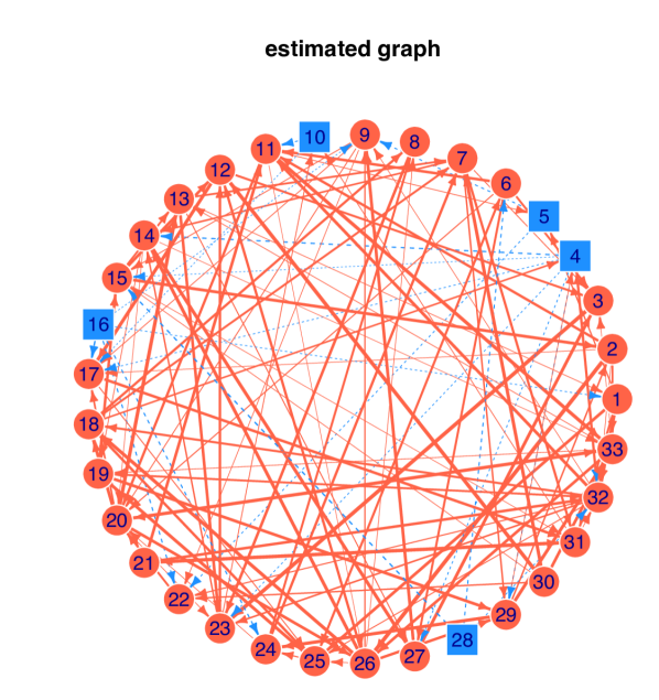
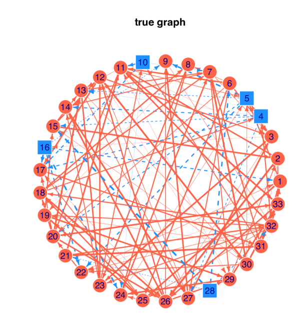
In Fig. 8, we present an example of estimation. The left graph shows the estimated connections W𝑊W and the right graph shows the true connections Wsuperscript𝑊W^{*}. The colors red and blue correspond to excitatory and inhibitory neurons, respectively, and the thickness of the edges represents the strength of the connections. The results confirm that the proposed method can extract the major connections successfully.
Refer to caption
Refer to caption
Figure 8: Example of the estimated graph W𝑊W and the true graph Wsuperscript𝑊W^{*}. The red circular nodes represent excitatory neurons and the red arrows represent excitatory connections. The blue square nodes represent inhibitory neurons and the blue dashed arrows represent inhibitory connections. The thickness of the arrows represents the strength of connections.

6.5.2 Network of 10,000 neurons

We generated one network. From this network, 20 different graphs consisting of 33 neurons were sampled. This simulation was performed to verify the proposed method under conditions comparable to real neuroscience experiments. Motivated by the result of the 100-neuron network, we set the size of the time window to Δ=10Δ10\Delta=10[ms]. We removed small values of the estimated connections W𝑊W and set the number of connections in W𝑊W to a pre-set value. Further, we assessed the performances by the correct detection of the strongest connections between observed neuron pairs. We systematically varied the number from the top 101010 connections to the top 100100100 connections. The sensitivity and Kendall rank correlation coefficient are plotted in Fig. 9 and Fig. 10, respectively, as functions of the number of connections. There are three box plots for each number of connections (from left to right, the results by Algorithm 2 and the estimated excitatory-inhibitory labels 𝒛𝒛\bm{z}, the cross-correlation function, and the binary logistic regression). In Fig. 9, we observe that the proposed method outperforms the other methods. In particular, on average, our method extracted 70%percent7070\% of the connections correctly, up to the top 20%percent2020\% of the connections. In terms of the Kendall rank correlation coefficient, as shown in Fig. 10, these three methods estimate the rank of connections nearly equally well.

We also investigated the sensitivity for excitatory and inhibitory connections separately. As shown in the left column of Fig. 11, the proposed method as well as logistic regression exhibited high sensitivity for excitatory connections. Specifically, the average sensitivity of the proposed method for the top 20 connections was greater than 75%percent7575\%. Song et al. (2005) demonstrated that the top 17%percent1717\% of synaptic connections contribute to half of the total connection strength. The result suggests that the proposed method detects the majority of the major excitatory connections successfully. Regarding inhibitory connections, as shown in the right column of Fig. 11, the proposed method clearly outperformed the other two methods. Such excellent performance is due to two features of the proposed method: removal of nuisance inputs and decomposition of pseudo-connections. In addition, we investigated how the proposed method estimates excitatory-inhibitory labels 𝒛𝒛\bm{z} in Fig. 12, in the same way as in Fig. 7. We found that many neuron types are estimated correctly in Fig. 12 left. We also confirmed that nearly all excitatory neurons are estimated correctly Fig. 12 right.

From an overall perspective, the numerical investigation using partially observed synthetic data demonstrated that the proposed method can detect both excitatory and inhibitory connections reliably.
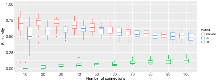
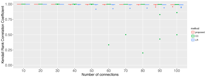
Refer to caption
Figure 9: Sensitivity measures to evaluate the performance of the proposed method in graphs composed of 33 neurons sampled from a network of 10,000 neurons. The horizontal axis represents the number of strongest connections from 10 to 100. There are three box plots for each connection number (from left to right, the results by Algorithm 2 and the estimated excitatory-inhibitory labels 𝒛𝒛\bm{z}, the cross-correlation function, and the binary logistic regression).
Refer to caption
Figure 10: Kendall rank correlation coefficient measures to evaluate the performance of the proposed method in graphs composed of 33 neurons sampled from a network of 10,000 neurons. The horizontal axis represents the number of strongest connections from 10 to 100. There are three box plots for each connection number (from left to right, the results by Algorithm 2 and the estimated excitatory-inhibitory labels 𝒛𝒛\bm{z}, the cross-correlation function, and the binary logistic regression.
Refer to caption
Figure 11: Sensitivity evaluated separately for excitatory and inhibitory connections in graphs composed of 33 neurons sampled from a network of 10,000 neurons. Left: the horizontal axis represents the number of strongest excitatory connections from 10 to 80. Right: the horizontal axis represents the number of strongest inhibitory connections from 5 to 20. There are three box plots for each connection number (from left to right, the results by Algorithm 2 and the estimated excitatory-inhibitory labels 𝒛𝒛\bm{z}, the cross-correlation function, and the binary logistic regression.
Refer to caption
Figure 12: Estimation of label 𝒛𝒛\bm{z} for 33 neurons sampled from a network of 10,000 neurons. Left: bar plot of the number of correctly estimated labels 𝒛𝒛\bm{z}. Right: estimated value of label 𝒛𝒛\bm{z} as a function of the sum of out-going connection weights of each neuron. The circles (\circ), plus signs, (++), triangles (\bigtriangleup), and crosses (×\times) represent correctly estimated excitatory neurons, incorrectly estimated excitatory neurons, correctly estimated inhibitory neurons, and incorrectly estimated inhibitory neurons, respectively.

7 Real data experiment

In this section, we apply the proposed method to electrophysiological data. We investigate whether the behaviorally induced effective connectivity assessed by the proposed method is sustained during a post-task sleep epoch.

7.1 Experiment outline

The electrophysiological data analyzed in this study were originally reported in Tatsuno et al. (2006). Briefly, an adult male brown Norway/Fischer 344 hybrid rat was used for 25 h of continuous recording. Based on the experimental protocol of Ribeiro et al. (2004), the recording sessions consisted of three epochs: a 12-h free-running pre-task epoch, a 1-h task epoch, and a 12-h post-task epoch. After implantation of the microdrive, the rat was housed in a recording box (height 42[cm], length 46.5[cm], and width 46.5[cm]) for at least 1 week before recording. This ensured that the animal was accustomed to the recording environment. Throughout the recording, the rat was allowed to move, eat, and sleep freely in the recording box, following its preferred sleep/wake cycle. During the task, the animal explored four novel objects located at each corner of the recording box. Encounters with these novel objects were considered novel experiences, as in a study by Ribeiro et al. (2004).

The recording was made by the microdrive with 12 independently adjustable tetrodes, covering a circular area of approximately 1 mm in diameter (Gothard et al., 1996). The drive was implanted above the hippocampus [3.8 mm posterior and 2.5 lateral (left) to the bregma], and lowered to the CA1 area. A reference electrode was implanted in the corpus callosum and an electrode for recording the hippocampal theta oscillation was implanted in the hippocampal fissure. The neural signals were bandpass filtered between 600 Hz and 6 kHz, and spike waveforms were recorded at 32 kHz whenever the signal exceeded a predetermined threshold. The recording of all data was performed using Cheetah Data Acquisition Systems (Neuralynx, Bozeman, MT, USA). The rat’s head position was identified by light emitting diodes on the microdrive and monitored by a color camera mounted on the ceiling of the recording room. The rat was also monitored by an infrared camera to allow for observation of behavior during the dark cycle. The video data were time-stamped and used for off-line detection of motion and motionless periods. To identify REM episodes within motionless periods, local field potential (LFP) traces were bandpass filtered in the delta (2–4 Hz) and theta (6–10 Hz) bands. The power in each band was computed and REM episodes were identified as periods of elevated theta-delta power ratio, such as >2.0absent2.0>2.0. The rest of the motionless periods was considered non-REM sleep. The units were isolated using a multidimensional cluster cutting software (MClust by A. D. Redish, University of Minnesota, Minneapolis, MN, USA). Only units with <1%absentpercent1<1\% of inter-spike-interval distribution falling within the 2 ms refractory period were used in the analysis. This process yielded 48 CA1 units. The type of neuron (excitatory or inhibitory) was estimated using the firing rate and spike width (Markus et al., 1994). For detection of effective connectivity by the proposed method, neurons with a low firing rate (<0.5absent0.5<0.5 Hz) were excluded because such neurons prevent reliable detection of connectivity.

7.2 Data analysis

7.2.1 Target data of interest

We focused on 5 h of recording data (2 h immediately before the task, 1 h of the task, and 2 hours immediately after the task) because memory replay of this type of spatial memory task is typically detected within 1 h after the task experience (Kudrimoti et al., 1999; Tatsuno et al., 2006). For analytical clarity, 2-h pre-task and post-task epochs were divided into approximately 1-h segments, respectively, which yielded 5 diagrams, as shown in Fig. 13. Following Wilson and McNaughton (1994), we analyzed the non-REM episodes during the pre-task and post-task epochs and the waking activity during task epoch.
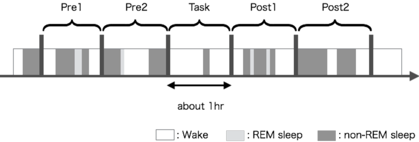
Refer to caption
Figure 13: Schematic illustration of electrophysiological data. The 5 h of spike data were divided into 5 segments of nearly equal duration: Pre1, Pre2, Task, Post1, and Post2. The colors white, light gray, and dark gray represent wake, REM sleep, and non-REM sleep epochs, respectively. Waking portions during the task epoch and non-REM portions during the pre-task and post-task epochs were used in the analysis.

7.2.2 Results

The size of the time window of the proposed method was set to 151515 ms on the basis of the spike-timing-dependent plasticity (STDP) window (Bi and Poo, 1998). Because the excitatory and inhibitory neurons were already estimated from the spike waveforms, we used the proposed method under the condition that the excitatory-inhibitory labels were already known. The estimated effective connectivity during the five segments is shown in the left column of Fig. 14. To quantify the similarity between waking and sleep epochs in the connection diagram, we defined the overlap rate o(p)superscript𝑜𝑝o^{(p)} for estimated connections {wij}i,jVsubscriptsubscript𝑤𝑖𝑗𝑖𝑗𝑉\{w_{ij}\}_{i,j\in V} by

o(p)=i,j(|sgn(wij)||sgn(w~ij(p))|)i,j|sgn(w~ij(p))|,superscript𝑜𝑝subscript𝑖𝑗sgnsubscript𝑤𝑖𝑗sgnsubscriptsuperscript~𝑤𝑝𝑖𝑗subscript𝑖𝑗sgnsubscriptsuperscript~𝑤𝑝𝑖𝑗\displaystyle o^{(p)}=\frac{\sum_{i,j}\Bigl{(}|{\rm sgn}(w_{ij})|\cdot|{\rm sgn}\bigl{(}\tilde{w}^{(p)}_{ij}\bigr{)}|\Bigr{)}}{\sum_{i,j}|{\rm sgn}\bigl{(}\tilde{w}^{(p)}_{ij}\bigr{)}|}, (73)

where sgn()sgn{\rm sgn}(\cdot) is the sign function. The top p%percent𝑝p\% connections {w~ij(p)}i,jVsubscriptsuperscriptsubscript~𝑤𝑖𝑗𝑝𝑖𝑗𝑉\{\tilde{w}_{ij}^{(p)}\}_{i,j\in V} during the task epoch were obtained by truncating the other weaker connections:

w~ij(p)={w~ijw~ij>ζ(p),0otherwise,subscriptsuperscript~𝑤𝑝𝑖𝑗casessubscript~𝑤𝑖𝑗subscript~𝑤𝑖𝑗superscript𝜁𝑝0otherwise\displaystyle\tilde{w}^{(p)}_{ij}=\begin{cases}\tilde{w}_{ij}&\tilde{w}_{ij}>\zeta^{(p)},\\ 0&\mbox{otherwise},\end{cases}

where ζ(p)superscript𝜁𝑝\zeta^{(p)} is the strength of the top p%percent𝑝p\% connections. Table 2 summarizes the overlap between the estimated connections during the task and during sleep epochs (Pre1, Pre2, Post1 and Post2). For the top 25%percent2525\% connections, the overlap rate of Post1 is the highest among the four sleep epochs; nearly half of the behaviorally induced connections remain during Post1. For the top 50%percent5050\% and 100%percent100100\%, the Post1 similarity is weakened, suggesting that the learned information is encoded by strong connections. The right column of Fig. 14 shows that new effective connections emerge on top of the existing stationary connections, and they are sustained during Post1. The result is also consistent with the previous finding that memory replay is typically observed within 30 min after the task training (Kudrimoti et al., 1999).

Table 2: Overlap rate of estimated connections between the task and sleep epochs.
p%percent𝑝p\% Pre1 Pre2 Post1 Post2
25%percent2525\% 0.286 0.200 0.429 0.229
50%percent5050\% 0.486 0.357 0.429 0.300
100%percent100100\% 0.471 0.364 0.450 0.336
Refer to caption
Figure 14: Estimated effective connectivity for each epoch. From top to bottom, each diagram represents the Pre1, Pre2, Task, Post1, and Post2 epoch, respectively. Left column: estimated effective connectivity drawn as in Fig. 8. Right column: the estimated effective connectivity drawn as by Wilson and McNaughton (1994). The red, green, and yellow lines represent connection weights of the top 25%percent2525\%, 50%percent5050\%, and 100%percent100100\%, respectively. The bold lines represent the connections that exist during the task and during either the pre-task or the post-task sleep epochs (Pre1, Pre2, Post1, and Post2).

8 Conclusion

In this paper, we proposed a novel method to estimate neural connections from partially observed spike trains. Specifically, we addressed three mathematical difficulties: influence of pseudo-correlations, influence from unobserved neurons, and estimation of excitatory and inhibitory neurons (hence, excitatory and inhibitory directed connections). The proposed method extracted the connections between the observed neurons by explicitly quantifying the influence from unobserved neurons. This was achieved by using the property of a sum of random variables and the assumption that nuisance inputs follow Gaussian distributions. Then, by modeling all possible spike propagations over multiple neurons, we eliminated the pseudo-correlations. Finally, we proposed a framework for estimating neuron types (excitatory or inhibitory) using the em𝑒𝑚em algorithm. Through numerical simulations, we confirmed that the proposed method can detect the major connection reliably for a small random network as well as for a large realistic network. In particular, for the estimation of inhibitory connections, the proposed method outperformed other standard methods, such as the cross-correlation function and binary logistic regression. In addition, we applied the method to multi-electrode data from the CA1 area of rat’s hippocampus. We found that the behavior-induced effective connections and the detected connections were sustained during the subsequent sleep.

The proposed method can be used for providing a macroscopic measure of connections within a temporal window of interest and for selecting specific connections for further analyses. However, note that it estimates averaged connections within a certain observation period specified by the width of the temporal window, but not dynamical connections. The validity of the average of neural connections is discussed in (Toyoizumi et al., 2009).

There are some issues that warrant further investigation. First, the proposed method tends to estimate inhibitory connections that are weaker than excitatory connections. This problem may arise from the same activation functions for both excitatory and inhibitory neurons even though they tend to fire at different frequencies. Separate activation functions may alleviate this problem. Second, in the present approach, the number of connections is given as an ad hoc parameter to the proposed algorithm. In other words, the proposed method does not have a mechanism to estimate the number of connections from each neuron. This could be determined by stability-based methods, such as StARS (Liu et al., 2010) and TIGRESS (Haury et al., 2012), but it should be noted that these methods tend to overestimate the number of connections. An important direction for future work is to develop an appropriate method to estimate the number of connections by considering the assumed signal propagation model.

Acknowledgements

Part of this work was supported by JSPS KAKENHI No.15H02669, 16K16108, 17H01793, and 25120009, and JST CREST ACA20935 and MJCR14D7.

Appendix A Proof of the property of the sum of random variables

A.1 Proof of Theorem 1

Let X𝑋X and Y𝑌Y be independent random variables with probability density functions fXsubscript𝑓𝑋f_{X} and fYsubscript𝑓𝑌f_{Y}, respectively. We show the proof of the property of the sum X+Y𝑋𝑌X+Y when 𝔼[Y]=0𝔼delimited-[]𝑌0\mathbb{E}[Y]=0. Consider any bonded function g𝑔g. The expectation of g(X+Y)𝑔𝑋𝑌g(X+Y) is represented by

𝔼[g(X+Y)]𝔼delimited-[]𝑔𝑋𝑌\displaystyle\mathbb{E}[g(X+Y)] =g(z)fX+Y(z)𝑑zabsent𝑔𝑧subscript𝑓𝑋𝑌𝑧differential-d𝑧\displaystyle=\int g(z)f_{X+Y}(z)dz
=g(z)[fX(x)fY(zx)𝑑x]𝑑zabsent𝑔𝑧delimited-[]subscript𝑓𝑋𝑥subscript𝑓𝑌𝑧𝑥differential-d𝑥differential-d𝑧\displaystyle=\int g(z)\Biggl{[}\int f_{X}(x)f_{Y}(z-x)dx\Biggr{]}dz
=fX(x)g(z)fY(zx)𝑑z𝑑x.absentdouble-integralsubscript𝑓𝑋𝑥𝑔𝑧subscript𝑓𝑌𝑧𝑥differential-d𝑧differential-d𝑥\displaystyle=\iint f_{X}(x)g(z)f_{Y}(z-x)dzdx. (74)

We define fY(x)=fY(x)subscriptsuperscript𝑓𝑌𝑥subscript𝑓𝑌𝑥f^{-}_{Y}(x)=f_{Y}(-x) and obtain

fX(x)g(z)fY(zx)𝑑z𝑑xdouble-integralsubscript𝑓𝑋𝑥𝑔𝑧subscript𝑓𝑌𝑧𝑥differential-d𝑧differential-d𝑥\displaystyle\iint f_{X}(x)g(z)f_{Y}(z-x)dzdx =fX(x)(g(z)fY(xz)𝑑z)𝑑xabsentsubscript𝑓𝑋𝑥𝑔𝑧subscriptsuperscript𝑓𝑌𝑥𝑧differential-d𝑧differential-d𝑥\displaystyle=\int f_{X}(x)\Biggl{(}\int g(z)f^{-}_{Y}(x-z)dz\Biggr{)}dx
=fX(x)h(x)𝑑xabsentsubscript𝑓𝑋𝑥𝑥differential-d𝑥\displaystyle=\int f_{X}(x)h(x)dx
=𝔼[h(X)],absent𝔼delimited-[]𝑋\displaystyle={\mathbb{E}}[h(X)], (75)

where h=gfY𝑔subscriptsuperscript𝑓𝑌h=g*f^{-}_{Y}, i.e., convolution of functions g𝑔g and fYsubscriptsuperscript𝑓𝑌f^{-}_{Y}. Thus, we get the following equation:

𝔼[g(X+Y)]=𝔼[h(X)].𝔼delimited-[]𝑔𝑋𝑌𝔼delimited-[]𝑋\displaystyle{\mathbb{E}}[g(X+Y)]={\mathbb{E}}[h(X)]. (76)

Then, we show the proof when 𝔼[Y]0𝔼delimited-[]𝑌0\mathbb{E}[Y]\neq 0. In this case, we transform variables X𝑋X and Y𝑌Y into Xsuperscript𝑋X^{\prime} and Ysuperscript𝑌Y^{\prime} as follows:

Xsuperscript𝑋\displaystyle X^{\prime} =X+𝔼[Y],absent𝑋𝔼delimited-[]𝑌\displaystyle=X+\mathbb{E}[Y],
Ysuperscript𝑌\displaystyle Y^{\prime} =Y𝔼[Y].absent𝑌𝔼delimited-[]𝑌\displaystyle=Y-\mathbb{E}[Y].

As with the proof when 𝔼[Y]=0𝔼delimited-[]𝑌0\mathbb{E}[Y]=0, we obtain

𝔼[g(X+Y)]𝔼delimited-[]𝑔𝑋𝑌\displaystyle{\mathbb{E}}[g(X+Y)] =𝔼[g((X+𝔼[Y])+(Y𝔼[Y]))]absent𝔼delimited-[]𝑔𝑋𝔼delimited-[]𝑌𝑌𝔼delimited-[]𝑌\displaystyle={\mathbb{E}}\Bigl{[}g\Bigl{(}(X+\mathbb{E}[Y])+(Y-\mathbb{E}[Y])\Bigr{)}\Bigr{]}
=𝔼[g(X+Y)]absent𝔼delimited-[]𝑔superscript𝑋superscript𝑌\displaystyle={\mathbb{E}}[g(X^{\prime}+Y^{\prime})]
=𝔼[h(X)].absent𝔼delimited-[]superscript𝑋\displaystyle={\mathbb{E}}[h(X^{\prime})]. (77)

Thus, we obtain the following equation:

𝔼[g(X+Y)]=𝔼[h(X+𝔼[Y])].𝔼delimited-[]𝑔𝑋𝑌𝔼delimited-[]𝑋𝔼delimited-[]𝑌\displaystyle{\mathbb{E}}[g(X+Y)]={\mathbb{E}}[h(X+\mathbb{E}[Y])]. (78)

A.2 Proof of Corollary 1

Assume that a function g𝑔g is Gaussian density function ϕσ2(x)=x𝒩(z;0,σ2)𝑑zsubscriptitalic-ϕsuperscript𝜎2𝑥superscriptsubscript𝑥𝒩𝑧0superscript𝜎2differential-d𝑧\phi_{\sigma^{2}}(x)=\int_{-\infty}^{x}\mathcal{N}(z;0,\sigma^{2})dz and fYsubscript𝑓𝑌f_{Y} is a Gaussian distribution with mean 𝔼[Y]𝔼delimited-[]𝑌\mathbb{E}[Y] and variance τ2superscript𝜏2\tau^{2}. The Gaussian density function is symmetric with 𝔼[Y]𝔼delimited-[]𝑌\mathbb{E}[Y]; hence, fY=fYsubscriptsuperscript𝑓𝑌subscript𝑓𝑌f^{-}_{Y}=f_{Y}. The convolution of g𝑔g and fYsubscriptsuperscript𝑓𝑌f^{-}_{Y} is represented by

gfY=ϕσ2ϕτ2=ϕσ2+τ2,𝑔subscriptsuperscript𝑓𝑌subscriptitalic-ϕsuperscript𝜎2subscriptitalic-ϕsuperscript𝜏2subscriptitalic-ϕsuperscript𝜎2superscript𝜏2\displaystyle g*f^{-}_{Y}=\phi_{\sigma^{2}}*\phi_{\tau^{2}}=\phi_{\sigma^{2}+\tau^{2}}, (79)

and we obtain

𝔼[ϕσ2(X+Y)]=ϕσ2+τ2(X+𝔼[Y]).𝔼delimited-[]subscriptitalic-ϕsuperscript𝜎2𝑋𝑌subscriptitalic-ϕsuperscript𝜎2superscript𝜏2𝑋𝔼delimited-[]𝑌\displaystyle\mathbb{E}[\phi_{\sigma^{2}}(X+Y)]=\phi_{\sigma^{2}+\tau^{2}}(X+\mathbb{E}[Y]). (80)

A.3 Proof of Theorem 2

Consider a cumulative distribution function G𝐺G of a probability density function g𝑔g. First, we show the following equation:

Gf(x)=xgf(z)𝑑z,𝐺𝑓𝑥superscriptsubscript𝑥𝑔𝑓𝑧differential-d𝑧\displaystyle G*f(x)=\int_{-\infty}^{x}g*f(z)dz, (81)

where f𝑓f is a probability density function. The right-hand side of the above equation is transformed as follows:

Gf(x)𝐺𝑓𝑥\displaystyle G*f(x) =G(y)f(xy)𝑑yabsent𝐺𝑦𝑓𝑥𝑦differential-d𝑦\displaystyle=\int G(y)f(x-y)dy
=g(z)𝟙y(z)f(xy)𝑑z𝑑y,absentdouble-integral𝑔𝑧subscriptdouble-struck-𝟙𝑦𝑧𝑓𝑥𝑦differential-d𝑧differential-d𝑦\displaystyle=\iint g(z)\mathbb{1}_{y}(z)f(x-y)dz\;dy, (82)

where 𝟙y(z),zsubscriptdouble-struck-𝟙𝑦𝑧𝑧\mathbb{1}_{y}(z),z\in\mathbb{R} is the following function:

𝟙y(z)={1,z<y,0,z>y.\displaystyle\mathbb{1}_{y}(z)=\left\{\begin{aligned} &1,\qquad&z<y,\\ &0,\qquad&z>y.\end{aligned}\right. (83)

We define w=xy𝑤𝑥𝑦w=x-y and obtain

g(z)𝟙y(z)f(xy)𝑑z𝑑ydouble-integral𝑔𝑧subscriptdouble-struck-𝟙𝑦𝑧𝑓𝑥𝑦differential-d𝑧differential-d𝑦\displaystyle\iint g(z)\mathbb{1}_{y}(z)f(x-y)dz\;dy =g(z)𝟙xw(z)f(w)𝑑z𝑑wz[,xw]formulae-sequenceabsentdouble-integral𝑔𝑧subscriptdouble-struck-𝟙𝑥𝑤𝑧𝑓𝑤differential-d𝑧differential-d𝑤𝑧𝑥𝑤\displaystyle=\iint g(z)\mathbb{1}_{x-w}(z)f(w)dz\;dw\qquad z\in[-\infty,x-w]
=xwg(z)f(w)𝑑z𝑑w.absentsuperscriptsubscriptsuperscriptsubscript𝑥𝑤𝑔𝑧𝑓𝑤differential-d𝑧differential-d𝑤\displaystyle=\int_{-\infty}^{\infty}\int_{-\infty}^{x-w}g(z)f(w)dz\;dw. (84)

On the other hand, the left-hand side of Eq. 81 is transformed as follows :

xgf(z)𝑑zsuperscriptsubscript𝑥𝑔𝑓𝑧differential-d𝑧\displaystyle\int_{-\infty}^{x}g*f(z)dz =xg(z)f(yz)𝑑z𝑑yabsentsuperscriptsubscript𝑥superscriptsubscript𝑔𝑧𝑓𝑦𝑧differential-d𝑧differential-d𝑦\displaystyle=\int_{-\infty}^{x}\int_{-\infty}^{\infty}g(z)f(y-z)dz\;dy
=g(z)f(yz)𝟙x(y)𝑑z𝑑y.absentdouble-integral𝑔𝑧𝑓𝑦𝑧subscriptdouble-struck-𝟙𝑥𝑦differential-d𝑧differential-d𝑦\displaystyle=\iint g(z)f(y-z)\mathbb{1}_{x}(y)dz\;dy. (85)

We define w=yz𝑤𝑦𝑧w=y-z and obtain

g(z)f(yz)𝟙x(y)𝑑z𝑑ydouble-integral𝑔𝑧𝑓𝑦𝑧subscriptdouble-struck-𝟙𝑥𝑦differential-d𝑧differential-d𝑦\displaystyle\iint g(z)f(y-z)\mathbb{1}_{x}(y)dz\;dy =g(z)f(w)𝟙x(w+z)𝑑z𝑑wabsentdouble-integral𝑔𝑧𝑓𝑤subscriptdouble-struck-𝟙𝑥𝑤𝑧differential-d𝑧differential-d𝑤\displaystyle=\iint g(z)f(w)\mathbb{1}_{x}(w+z)dz\;dw
=xwg(z)f(w)𝑑z𝑑w.absentsuperscriptsubscriptsuperscriptsubscript𝑥𝑤𝑔𝑧𝑓𝑤differential-d𝑧differential-d𝑤\displaystyle=\int_{-\infty}^{\infty}\int_{-\infty}^{x-w}g(z)f(w)dz\;dw. (86)

Eq. 84 coincides with Eq. 86 and it proves Eq. 81. By applying Theorem 1 to the expectation of G(X+Y)𝐺𝑋𝑌G(X+Y), we get the following equation :

𝔼[G(X+Y)]𝔼delimited-[]𝐺𝑋𝑌\displaystyle\mathbb{E}[G(X+Y)] =𝔼[H(X+𝔼[Y])],absent𝔼delimited-[]𝐻𝑋𝔼delimited-[]𝑌\displaystyle=\mathbb{E}[H(X+\mathbb{E}[Y])], (87)

where H(x)=(GfY)(x)=x(gfY)(z)𝑑z𝐻𝑥𝐺subscriptsuperscript𝑓𝑌𝑥superscriptsubscript𝑥𝑔subscriptsuperscript𝑓𝑌𝑧differential-d𝑧H(x)=(G*f^{-}_{Y})(x)=\int_{-\infty}^{x}(g*f^{-}_{Y})(z)dz.

A.4 Proof of Corollary 2

Consider the case G(x)=Φσ2(x)=ϕσ2(z)𝑑z𝐺𝑥subscriptΦsuperscript𝜎2𝑥subscriptitalic-ϕsuperscript𝜎2𝑧differential-d𝑧G(x)=\Phi_{\sigma^{2}}(x)=\int\phi_{\sigma^{2}}(z)dz and let fYsubscript𝑓𝑌f_{Y} be a Gaussian distribution with mean 𝔼[Y]𝔼delimited-[]𝑌\mathbb{E}[Y] and variance τ2superscript𝜏2\tau^{2}. The convolution of G𝐺G and fYsubscriptsuperscript𝑓𝑌f^{-}_{Y} is represented by

(GfY)(x)𝐺subscriptsuperscript𝑓𝑌𝑥\displaystyle(G*f^{-}_{Y})(x) =x(gfY)(z)𝑑zabsentsuperscriptsubscript𝑥𝑔subscriptsuperscript𝑓𝑌𝑧differential-d𝑧\displaystyle=\int_{-\infty}^{x}(g*f^{-}_{Y})(z)dz
=x(ϕσ2ϕτ2)(z)𝑑zabsentsuperscriptsubscript𝑥subscriptitalic-ϕsuperscript𝜎2subscriptitalic-ϕsuperscript𝜏2𝑧differential-d𝑧\displaystyle=\int_{-\infty}^{x}(\phi_{\sigma^{2}}*\phi_{\tau^{2}})(z)dz
=xϕσ2+τ2(z)𝑑zabsentsuperscriptsubscript𝑥subscriptitalic-ϕsuperscript𝜎2superscript𝜏2𝑧differential-d𝑧\displaystyle=\int_{-\infty}^{x}\phi_{\sigma^{2}+\tau^{2}}(z)dz
=Φσ2+τ2(x).absentsubscriptΦsuperscript𝜎2superscript𝜏2𝑥\displaystyle=\Phi_{\sigma^{2}+\tau^{2}}(x). (88)

Therefore, we obtain

𝔼[Φσ2(X+Y)]=Φσ2+τ2(X+𝔼[Y]).𝔼delimited-[]subscriptΦsuperscript𝜎2𝑋𝑌subscriptΦsuperscript𝜎2superscript𝜏2𝑋𝔼delimited-[]𝑌\displaystyle\mathbb{E}[\Phi_{\sigma^{2}}(X+Y)]=\Phi_{\sigma^{2}+\tau^{2}}(X+\mathbb{E}[Y]). (89)

Appendix B Derivation of projection steps in the em𝑒𝑚em algorithm to estimate excitatory probability

B.1 Derivation of the projection from 𝒟𝒟\mathcal{D} to 𝒟superscript𝒟\mathcal{D}^{\prime}

Consider the e𝑒e-projection from 𝒟𝒟\mathcal{D} to 𝒟superscript𝒟\mathcal{D}^{\prime}:

𝜷(τ+1)=missingargmin𝜷DKL[q(Λ,𝒛;𝜷),q(Λ,𝒛;𝜶(τ))].superscript𝜷𝜏1missing𝑎𝑟𝑔𝑚𝑖subscript𝑛𝜷subscript𝐷KLsuperscript𝑞Λ𝒛𝜷𝑞Λ𝒛superscript𝜶𝜏\displaystyle\bm{\beta}^{(\tau+1)}=\mathop{\mathrm{missing}}{argmin}\limits_{\bm{\beta}}D_{\mathrm{KL}}[q^{\prime}(\Lambda,\bm{z};\bm{\beta}),q(\Lambda,\bm{z};\bm{\alpha}^{(\tau)})]. (90)

Substituting p(Λ,𝒛;𝜶(τ))𝑝Λ𝒛superscript𝜶𝜏p(\Lambda,\bm{z};\bm{\alpha}^{(\tau)}) with q(Λ,𝒛;𝜶(τ))𝑞Λ𝒛superscript𝜶𝜏q(\Lambda,\bm{z};\bm{\alpha}^{(\tau)}) in the previous projection step, the above equation is equivalent to

𝜷(τ+1)superscript𝜷𝜏1\displaystyle\bm{\beta}^{(\tau+1)} =missingargmin𝜷DKL[q(𝒛Λ;𝜷),p(𝒛Λ;𝜶(τ))]absentmissing𝑎𝑟𝑔𝑚𝑖subscript𝑛𝜷subscript𝐷KLsuperscript𝑞conditional𝒛Λ𝜷𝑝conditional𝒛Λsuperscript𝜶𝜏\displaystyle=\mathop{\mathrm{missing}}{argmin}\limits_{\bm{\beta}}D_{\mathrm{KL}}[q^{\prime}(\bm{z}\mid\Lambda;\bm{\beta}),p(\bm{z}\mid\Lambda;\bm{\alpha}^{(\tau)})]
=missingargmin𝜷𝒛q(𝒛Λ;𝜷)logq(𝒛Λ;𝜷)q(𝒛Λ;𝜷)logp(𝒛Λ;𝜶(τ))absentmissing𝑎𝑟𝑔𝑚𝑖subscript𝑛𝜷subscript𝒛superscript𝑞conditional𝒛Λ𝜷superscript𝑞conditional𝒛Λ𝜷superscript𝑞conditional𝒛Λ𝜷𝑝conditional𝒛Λsuperscript𝜶𝜏\displaystyle=\mathop{\mathrm{missing}}{argmin}\limits_{\bm{\beta}}\sum_{\bm{z}}q^{\prime}(\bm{z}\mid\Lambda;\bm{\beta})\log{q^{\prime}(\bm{z}\mid\Lambda;\bm{\beta})}-q^{\prime}(\bm{z}\mid\Lambda;\bm{\beta})\log{p(\bm{z}\mid\Lambda;\bm{\alpha}^{(\tau)})}
=missingargmin𝜷𝒛{i=1Nβizi(1βi)1zilogi=1Nβizi(1βi)1zi\displaystyle=\mathop{\mathrm{missing}}{argmin}\limits_{\bm{\beta}}\sum_{\bm{z}}\Bigl{\{}\prod_{i=1}^{N}\beta_{i}^{z_{i}}(1-\beta_{i})^{1-z_{i}}\log{\prod_{i=1}^{N}\beta_{i}^{z_{i}}(1-\beta_{i})^{1-z_{i}}}
i=1Nβizi(1βi)1zilogp(𝒛Λ;𝜶(τ))}\displaystyle\qquad\qquad\qquad-\prod_{i=1}^{N}\beta_{i}^{z_{i}}(1-\beta_{i})^{1-z_{i}}\log{p(\bm{z}\mid\Lambda;\bm{\alpha}^{(\tau)})}\Bigr{\}}
=missingargmin𝜷𝒛[i=1Nβizi(1βi)1zi{logi=1Nβizi(1βi)1zilogp(𝒛Λ;𝜶(τ))}].absentmissing𝑎𝑟𝑔𝑚𝑖subscript𝑛𝜷subscript𝒛delimited-[]superscriptsubscriptproduct𝑖1𝑁superscriptsubscript𝛽𝑖subscript𝑧𝑖superscript1subscript𝛽𝑖1subscript𝑧𝑖superscriptsubscriptproduct𝑖1𝑁superscriptsubscript𝛽𝑖subscript𝑧𝑖superscript1subscript𝛽𝑖1subscript𝑧𝑖𝑝conditional𝒛Λsuperscript𝜶𝜏\displaystyle=\mathop{\mathrm{missing}}{argmin}\limits_{\bm{\beta}}\sum_{\bm{z}}\Biggl{[}\prod_{i=1}^{N}\beta_{i}^{z_{i}}(1-\beta_{i})^{1-z_{i}}\Biggl{\{}\log{\prod_{i=1}^{N}\beta_{i}^{z_{i}}(1-\beta_{i})^{1-z_{i}}}-\log{p(\bm{z}\mid\Lambda;\bm{\alpha}^{(\tau)})}\Biggr{\}}\Biggr{]}. (91)

Here, we define

q(𝒛iΛ,𝜷)=jiβjzj(1βj)1zjsuperscript𝑞conditionalsubscript𝒛𝑖Λ𝜷subscriptproduct𝑗𝑖superscriptsubscript𝛽𝑗subscript𝑧𝑗superscript1subscript𝛽𝑗1subscript𝑧𝑗\displaystyle q^{\prime}(\bm{z}_{-i}\mid\Lambda,\bm{\beta})=\prod_{j\neq i}\beta_{j}^{z_{j}}(1-\beta_{j})^{1-z_{j}}

and partially differentiate the terms in Eq. 91 with the parameter βisubscript𝛽𝑖\beta_{i}.

βii=1Nβizi(1βi)1zi=q(𝒛iΛ,𝜷){zi(1βiβi)1zi(1zi)(βi1βi)zi}subscript𝛽𝑖superscriptsubscriptproduct𝑖1𝑁superscriptsubscript𝛽𝑖subscript𝑧𝑖superscript1subscript𝛽𝑖1subscript𝑧𝑖superscript𝑞conditionalsubscript𝒛𝑖Λ𝜷subscript𝑧𝑖superscript1subscript𝛽𝑖subscript𝛽𝑖1subscript𝑧𝑖1subscript𝑧𝑖superscriptsubscript𝛽𝑖1subscript𝛽𝑖subscript𝑧𝑖\displaystyle\frac{\partial}{\partial\beta_{i}}\prod_{i=1}^{N}\beta_{i}^{z_{i}}(1-\beta_{i})^{1-z_{i}}=q^{\prime}(\bm{z}_{-i}\mid\Lambda,\bm{\beta})\Biggl{\{}z_{i}\Bigl{(}\frac{1-\beta_{i}}{\beta_{i}}\Bigr{)}^{1-z_{i}}-(1-z_{i})\Bigl{(}\frac{\beta_{i}}{1-\beta_{i}}\Bigr{)}^{z_{i}}\Biggr{\}}
βi{logi=1Nβizi(1βi)1zilogp(𝒛Λ;𝜶(τ))}=ziβi1zi1βi.subscript𝛽𝑖superscriptsubscriptproduct𝑖1𝑁superscriptsubscript𝛽𝑖subscript𝑧𝑖superscript1subscript𝛽𝑖1subscript𝑧𝑖𝑝conditional𝒛Λsuperscript𝜶𝜏subscript𝑧𝑖subscript𝛽𝑖1subscript𝑧𝑖1subscript𝛽𝑖\displaystyle\frac{\partial}{\partial\beta_{i}}\Biggl{\{}\log{\prod_{i=1}^{N}\beta_{i}^{z_{i}}(1-\beta_{i})^{1-z_{i}}}-\log{p(\bm{z}\mid\Lambda;\bm{\alpha}^{(\tau)})}\Biggr{\}}=\frac{z_{i}}{\beta_{i}}-\frac{1-z_{i}}{1-\beta_{i}}.

Thus, we solve Eq. 91 as follows:

00\displaystyle 0 =βi𝒛[i=1Nβizi(1βi)1zilogq(𝒛Λ;𝜷)p(𝒛Λ;𝜶(τ))]absentsubscript𝛽𝑖subscript𝒛delimited-[]superscriptsubscriptproduct𝑖1𝑁superscriptsubscript𝛽𝑖subscript𝑧𝑖superscript1subscript𝛽𝑖1subscript𝑧𝑖superscript𝑞conditional𝒛Λ𝜷𝑝conditional𝒛Λsuperscript𝜶𝜏\displaystyle=\frac{\partial}{\partial\beta_{i}}\sum_{\bm{z}}\Biggl{[}\prod_{i=1}^{N}\beta_{i}^{z_{i}}(1-\beta_{i})^{1-z_{i}}\log{\frac{q^{\prime}(\bm{z}\mid\Lambda;\bm{\beta})}{p(\bm{z}\mid\Lambda;\bm{\alpha}^{(\tau)})}}\Biggr{]}
=𝒛[q(𝒛iΛ,𝜷){zi(1βiβi)1zi(1zi)(βi1βi)zi}{logq(𝒛Λ;𝜷)p(𝒛Λ;𝜶(τ))}\displaystyle=\sum_{\bm{z}}\!\Biggl{[}q^{\prime}(\bm{z}_{-i}\mid\Lambda,\bm{\beta})\Biggl{\{}z_{i}\!\Bigl{(}\frac{1\!-\!\beta_{i}}{\beta_{i}}\Bigr{)}^{1\!-\!z_{i}}\!-\!(1\!-\!z_{i})\Bigl{(}\frac{\beta_{i}}{1\!-\!\beta_{i}}\Bigr{)}^{z_{i}}\Biggr{\}}\Biggl{\{}\log{\frac{q^{\prime}(\bm{z}\!\mid\!\Lambda;\!\bm{\beta})}{p(\bm{z}\!\mid\!\Lambda;\!\bm{\alpha}^{(\tau)})}}\Biggr{\}}
+q(𝒛iΛ,𝜷)βizi(1βi)1zi{ziβi1zi1βi}]\displaystyle\qquad\qquad+\!q^{\prime}(\bm{z}_{-i}\mid\Lambda,\bm{\beta})\beta_{i}^{z_{i}}(1\!-\!\beta_{i})^{1\!-\!z_{i}}\Biggl{\{}\frac{z_{i}}{\beta_{i}}\!-\!\frac{1\!-\!z_{i}}{1\!-\!\beta_{i}}\Biggr{\}}\Biggr{]}
=𝒛[q(𝒛iΛ,𝜷){zi(1βiβi)1zi(1zi)(βi1βi)zi}{logq(𝒛Λ;𝜷)p(𝒛Λ;𝜶(τ))}\displaystyle=\sum_{\bm{z}}\!\Biggl{[}q^{\prime}(\bm{z}_{-i}\mid\Lambda,\bm{\beta})\Biggl{\{}z_{i}\!\Bigl{(}\frac{1\!-\!\beta_{i}}{\beta_{i}}\Bigr{)}^{1\!-\!z_{i}}\!-\!(1\!-\!z_{i})\Bigl{(}\frac{\beta_{i}}{1\!-\!\beta_{i}}\Bigr{)}^{z_{i}}\Biggr{\}}\Biggl{\{}\log{\frac{q^{\prime}(\bm{z}\!\mid\!\Lambda;\!\bm{\beta})}{p(\bm{z}\!\mid\!\Lambda;\!\bm{\alpha}^{(\tau)})}}\Biggr{\}}
+q(𝒛iΛ,𝜷){zi(1βiβi)1zi(1zi)(βi1βi)zi}]\displaystyle\qquad\qquad+q^{\prime}(\bm{z}_{-i}\mid\Lambda,\bm{\beta})\Biggl{\{}z_{i}\!\Bigl{(}\frac{1\!-\!\beta_{i}}{\beta_{i}}\Bigr{)}^{1\!-\!z_{i}}\!-\!(1\!-\!z_{i})\Bigl{(}\frac{\beta_{i}}{1\!-\!\beta_{i}}\Bigr{)}^{z_{i}}\!\Biggr{\}}\Biggr{]}
=𝒛[q(𝒛iΛ,𝜷){zi(1βiβi)1zi(1zi)(βi1βi)zi}{logq(𝒛Λ;𝜷)p(𝒛Λ;𝜶(τ))+1}].absentsubscript𝒛delimited-[]superscript𝑞conditionalsubscript𝒛𝑖Λ𝜷subscript𝑧𝑖superscript1subscript𝛽𝑖subscript𝛽𝑖1subscript𝑧𝑖1subscript𝑧𝑖superscriptsubscript𝛽𝑖1subscript𝛽𝑖subscript𝑧𝑖superscript𝑞conditional𝒛Λ𝜷𝑝conditional𝒛Λsuperscript𝜶𝜏1\displaystyle=\sum_{\bm{z}}\!\Biggl{[}q^{\prime}(\bm{z}_{-i}\mid\Lambda,\bm{\beta})\Biggl{\{}z_{i}\!\Bigl{(}\frac{1\!-\!\beta_{i}}{\beta_{i}}\Bigr{)}^{1\!-\!z_{i}}\!-\!(1\!-\!z_{i})\Bigl{(}\frac{\beta_{i}}{1\!-\!\beta_{i}}\Bigr{)}^{z_{i}}\Biggr{\}}\Biggl{\{}\log{\frac{q^{\prime}(\bm{z}\!\mid\!\Lambda;\!\bm{\beta})}{p(\bm{z}\!\mid\!\Lambda;\!\bm{\alpha}^{(\tau)})}}\!+\!1\Biggr{\}}\Biggr{]}.

Therefore, the above equation becomes

𝒛q(𝒛iΛ,𝜷)zi(1βiβi)1zi{logq(𝒛Λ;𝜷)p(𝒛Λ;𝜶(τ))+1}subscript𝒛superscript𝑞conditionalsubscript𝒛𝑖Λ𝜷subscript𝑧𝑖superscript1subscript𝛽𝑖subscript𝛽𝑖1subscript𝑧𝑖superscript𝑞conditional𝒛Λ𝜷𝑝conditional𝒛Λsuperscript𝜶𝜏1\displaystyle\sum_{\bm{z}}q^{\prime}(\bm{z}_{-i}\mid\Lambda,\bm{\beta})z_{i}\Bigl{(}\frac{1-\beta_{i}}{\beta_{i}}\Bigr{)}^{1-z_{i}}\Biggl{\{}\log{\frac{q^{\prime}(\bm{z}\mid\Lambda;\bm{\beta})}{p(\bm{z}\mid\Lambda;\bm{\alpha}^{(\tau)})}}+1\Biggr{\}}
=𝒛q(𝒛iΛ,𝜷)(1zi)(βi1βi)zi{logq(𝒛Λ;𝜷)p(𝒛Λ;𝜶(τ))+1}absentsubscript𝒛superscript𝑞conditionalsubscript𝒛𝑖Λ𝜷1subscript𝑧𝑖superscriptsubscript𝛽𝑖1subscript𝛽𝑖subscript𝑧𝑖superscript𝑞conditional𝒛Λ𝜷𝑝conditional𝒛Λsuperscript𝜶𝜏1\displaystyle\qquad\qquad=\sum_{\bm{z}}q^{\prime}(\bm{z}_{-i}\mid\Lambda,\bm{\beta})(1-z_{i})\Bigl{(}\frac{\beta_{i}}{1-\beta_{i}}\Bigr{)}^{z_{i}}\Biggl{\{}\log{\frac{q^{\prime}(\bm{z}\mid\Lambda;\bm{\beta})}{p(\bm{z}\mid\Lambda;\bm{\alpha}^{(\tau)})}}+1\Biggr{\}}
\displaystyle\Leftrightarrow 𝒛iq(𝒛iΛ,𝜷){logq(𝒛iΛ,zi=1;𝜷)p(𝒛iΛ,zi=1;𝜶(τ))+1}subscriptsubscript𝒛𝑖superscript𝑞conditionalsubscript𝒛𝑖Λ𝜷superscript𝑞conditionalsubscript𝒛𝑖Λsubscript𝑧𝑖1𝜷𝑝conditionalsubscript𝒛𝑖Λsubscript𝑧𝑖1superscript𝜶𝜏1\displaystyle\sum_{\bm{z}_{-i}}q^{\prime}(\bm{z}_{-i}\mid\Lambda,\bm{\beta})\Biggl{\{}\log{\frac{q^{\prime}(\bm{z}_{-i}\mid\Lambda,z_{i}=1;\bm{\beta})}{p(\bm{z}_{-i}\mid\Lambda,z_{i}=1;\bm{\alpha}^{(\tau)})}}+1\Biggr{\}}
=𝒛iq(𝒛iΛ,𝜷){logq(𝒛iΛ,zi=0;𝜷)p(𝒛iΛ,zi=0;𝜶(τ))+1}absentsubscriptsubscript𝒛𝑖superscript𝑞conditionalsubscript𝒛𝑖Λ𝜷superscript𝑞conditionalsubscript𝒛𝑖Λsubscript𝑧𝑖0𝜷𝑝conditionalsubscript𝒛𝑖Λsubscript𝑧𝑖0superscript𝜶𝜏1\displaystyle\qquad\qquad=\sum_{\bm{z}_{-i}}q^{\prime}(\bm{z}_{-i}\mid\Lambda,\bm{\beta})\Biggl{\{}\log{\frac{q^{\prime}(\bm{z}_{-i}\mid\Lambda,z_{i}=0;\bm{\beta})}{p(\bm{z}_{-i}\mid\Lambda,z_{i}=0;\bm{\alpha}^{(\tau)})}}+1\Biggr{\}}
\displaystyle\Leftrightarrow 𝒛iq(𝒛iΛ,𝜷)logq(𝒛iΛ,zi=1;𝜷)q(𝒛iΛ,zi=0;𝜷)subscriptsubscript𝒛𝑖superscript𝑞conditionalsubscript𝒛𝑖Λ𝜷superscript𝑞conditionalsubscript𝒛𝑖Λsubscript𝑧𝑖1𝜷superscript𝑞conditionalsubscript𝒛𝑖Λsubscript𝑧𝑖0𝜷\displaystyle\sum_{\bm{z}_{-i}}q^{\prime}(\bm{z}_{-i}\mid\Lambda,\bm{\beta})\log{\frac{q^{\prime}(\bm{z}_{-i}\mid\Lambda,z_{i}=1;\bm{\beta})}{q^{\prime}(\bm{z}_{-i}\mid\Lambda,z_{i}=0;\bm{\beta})}}
=𝒛iq(𝒛iΛ,𝜷)logp(𝒛iΛ,zi=1;𝜶(τ))p(𝒛iΛ,zi=0;𝜶(τ))absentsubscriptsubscript𝒛𝑖superscript𝑞conditionalsubscript𝒛𝑖Λ𝜷𝑝conditionalsubscript𝒛𝑖Λsubscript𝑧𝑖1superscript𝜶𝜏𝑝conditionalsubscript𝒛𝑖Λsubscript𝑧𝑖0superscript𝜶𝜏\displaystyle\qquad\qquad=\sum_{\bm{z}_{-i}}q^{\prime}(\bm{z}_{-i}\mid\Lambda,\bm{\beta})\log{\frac{p(\bm{z}_{-i}\mid\Lambda,z_{i}=1;\bm{\alpha}^{(\tau)})}{p(\bm{z}_{-i}\mid\Lambda,z_{i}=0;\bm{\alpha}^{(\tau)})}}
\displaystyle\Leftrightarrow logβi1βi=𝒛iq(𝒛iΛ,𝜷)logp(𝒛iΛ,zi=1;𝜶(τ))p(𝒛iΛ,zi=0;𝜶(τ)).subscript𝛽𝑖1subscript𝛽𝑖subscriptsubscript𝒛𝑖superscript𝑞conditionalsubscript𝒛𝑖Λ𝜷continued-fraction𝑝conditionalsubscript𝒛𝑖Λsubscript𝑧𝑖1superscript𝜶𝜏𝑝conditionalsubscript𝒛𝑖Λsubscript𝑧𝑖0superscript𝜶𝜏\displaystyle\log{\frac{\beta_{i}}{1-\beta_{i}}}=\sum_{\bm{z}_{-i}}q^{\prime}(\bm{z}_{-i}\mid\Lambda,\bm{\beta})\log{\cfrac{p(\bm{z}_{-i}\mid\Lambda,z_{i}=1;\bm{\alpha}^{(\tau)})}{p(\bm{z}_{-i}\mid\Lambda,z_{i}=0;\bm{\alpha}^{(\tau)})}}. (92)

Thus, we define the right-hand side in the above equation as A(τ)superscript𝐴𝜏A^{(\tau)} and obtain

βi(τ+1)11+exp{A(τ)}.superscriptsubscript𝛽𝑖𝜏1continued-fraction11superscript𝐴𝜏\displaystyle\beta_{i}^{(\tau+1)}\leftarrow\cfrac{1}{1+\exp{\bigl{\{}-A^{(\tau)}\bigr{\}}}}. (93)

B.2 Derivation of the projection from 𝒟superscript𝒟\mathcal{D}^{\prime} to superscript\mathcal{M}^{\prime}

We consider m𝑚m-projection from 𝒟superscript𝒟\mathcal{D}^{\prime} to superscript\mathcal{M}^{\prime}:

𝜶(τ+1)=missingargmin𝜶DKL[q(Λ,𝒛;𝜷(τ)),p(Λ,𝒛;𝜶)].superscript𝜶𝜏1missing𝑎𝑟𝑔𝑚𝑖subscript𝑛𝜶subscript𝐷KLsuperscript𝑞Λ𝒛superscript𝜷𝜏𝑝Λ𝒛𝜶\displaystyle\bm{\alpha}^{(\tau+1)}=\mathop{\mathrm{missing}}{argmin}\limits_{\bm{\alpha}}D_{\mathrm{KL}}[q^{\prime}(\Lambda,\bm{z};\bm{\beta}^{(\tau)}),p(\Lambda,\bm{z};\bm{\alpha})]. (94)

The KL divergence is explicitly given by

DKL[q(Λ,𝒛;𝜷(τ)),p(Λ,𝒛;𝜶)]subscript𝐷KLsuperscript𝑞Λ𝒛superscript𝜷𝜏𝑝Λ𝒛𝜶\displaystyle D_{\mathrm{KL}}[q^{\prime}(\Lambda,\bm{z};\bm{\beta}^{(\tau)}),p(\Lambda,\bm{z};\bm{\alpha})]
=Λ𝒛{q(Λ,𝒛;𝜷(τ))logq(Λ,𝒛;𝜷(τ))\displaystyle=\sum_{\Lambda}\sum_{\bm{z}}\Bigr{\{}q^{\prime}(\Lambda,\bm{z};\bm{\beta}^{(\tau)})\log{q^{\prime}(\Lambda,\bm{z};\bm{\beta}^{(\tau)})}
q(Λ,𝒛;𝜷(τ))logp(Λ,𝒛;𝜶)}.\displaystyle\qquad\qquad\qquad-q^{\prime}(\Lambda,\bm{z};\bm{\beta}^{(\tau)})\log{p(\Lambda,\bm{z};\bm{\alpha})}\Bigr{\}}. (95)

Therefore, the minimization in Eq. 94 is equivalent to the following maximization:

𝜶(τ+1)superscript𝜶𝜏1\displaystyle\bm{\alpha}^{(\tau+1)} =missingargmax𝜶Λ𝒛q(Λ,𝒛;𝜷(τ))logp(Λ,𝒛;𝜶)absentmissing𝑎𝑟𝑔𝑚𝑎subscript𝑥𝜶subscriptΛsubscript𝒛superscript𝑞Λ𝒛superscript𝜷𝜏𝑝Λ𝒛𝜶\displaystyle=\mathop{\mathrm{missing}}{argmax}\limits_{\bm{\alpha}}\sum_{\Lambda}\sum_{\bm{z}}q^{\prime}(\Lambda,\bm{z};\bm{\beta}^{(\tau)})\log{p(\Lambda,\bm{z};\bm{\alpha})}
=missingargmax𝜶Λ𝒛q(Λ)q(𝒛Λ;𝜷(τ))logp(Λ𝒛)p(𝒛;𝜶)absentmissing𝑎𝑟𝑔𝑚𝑎subscript𝑥𝜶subscriptΛsubscript𝒛superscript𝑞Λsuperscript𝑞conditional𝒛Λsuperscript𝜷𝜏𝑝conditionalΛ𝒛𝑝𝒛𝜶\displaystyle=\mathop{\mathrm{missing}}{argmax}\limits_{\bm{\alpha}}\sum_{\Lambda}\sum_{\bm{z}}q^{\prime}(\Lambda)q^{\prime}(\bm{z}\mid\Lambda;\bm{\beta}^{(\tau)})\log{p(\Lambda\mid\bm{z})p(\bm{z};\bm{\alpha})}
=missingargmax𝜶Λ𝒛q(Λ)q(𝒛Λ;𝜷(τ))logp(𝒛;𝜶)absentmissing𝑎𝑟𝑔𝑚𝑎subscript𝑥𝜶subscriptΛsubscript𝒛superscript𝑞Λsuperscript𝑞conditional𝒛Λsuperscript𝜷𝜏𝑝𝒛𝜶\displaystyle=\mathop{\mathrm{missing}}{argmax}\limits_{\bm{\alpha}}\sum_{\Lambda}\sum_{\bm{z}}q^{\prime}(\Lambda)q^{\prime}(\bm{z}\mid\Lambda;\bm{\beta}^{(\tau)})\log{p(\bm{z};\bm{\alpha})}
=missingargmax𝜶Λq(Λ)𝒛q(𝒛Λ;𝜷(τ))logj=1Np(zj;αj)absentmissing𝑎𝑟𝑔𝑚𝑎subscript𝑥𝜶subscriptΛsuperscript𝑞Λsubscript𝒛superscript𝑞conditional𝒛Λsuperscript𝜷𝜏superscriptsubscriptproduct𝑗1𝑁𝑝subscript𝑧𝑗subscript𝛼𝑗\displaystyle=\mathop{\mathrm{missing}}{argmax}\limits_{\bm{\alpha}}\sum_{\Lambda}q^{\prime}(\Lambda)\sum_{\bm{z}}q^{\prime}(\bm{z}\mid\Lambda;\bm{\beta}^{(\tau)})\log{\prod_{j=1}^{N}p(z_{j};\alpha_{j})}
=missingargmax𝜶𝒛q(𝒛Λ;𝜷(τ))j=1Nlogp(zj;αj).absentmissing𝑎𝑟𝑔𝑚𝑎subscript𝑥𝜶subscript𝒛superscript𝑞conditional𝒛Λsuperscript𝜷𝜏superscriptsubscript𝑗1𝑁𝑝subscript𝑧𝑗subscript𝛼𝑗\displaystyle=\mathop{\mathrm{missing}}{argmax}\limits_{\bm{\alpha}}\sum_{\bm{z}}q^{\prime}(\bm{z}\mid\Lambda;\bm{\beta}^{(\tau)})\sum_{j=1}^{N}\log{p(z_{j};\alpha_{j})}. (96)

Partial differentiation of the right-hand side of Eq.96 with respect to αisubscript𝛼𝑖\alpha_{i} gives

00\displaystyle 0 =αi{𝒛q(𝒛Λ;𝜷(τ))j=1Nlogp(zj;αj)}absentsubscript𝛼𝑖subscript𝒛superscript𝑞conditional𝒛Λsuperscript𝜷𝜏superscriptsubscript𝑗1𝑁𝑝subscript𝑧𝑗subscript𝛼𝑗\displaystyle=\frac{\partial}{\partial\alpha_{i}}\Bigl{\{}\sum_{\bm{z}}q^{\prime}(\bm{z}\mid\Lambda;\bm{\beta}^{(\tau)})\sum_{j=1}^{N}\log{p(z_{j};\alpha_{j})}\Bigr{\}}
=𝒛q(𝒛Λ;𝜷(τ)){ziαi1zi1αi}.absentsubscript𝒛superscript𝑞conditional𝒛Λsuperscript𝜷𝜏subscript𝑧𝑖subscript𝛼𝑖1subscript𝑧𝑖1subscript𝛼𝑖\displaystyle=\sum_{\bm{z}}q^{\prime}(\bm{z}\mid\Lambda;\bm{\beta}^{(\tau)})\Bigl{\{}\frac{z_{i}}{\alpha_{i}}-\frac{1-z_{i}}{1-\alpha_{i}}\Bigr{\}}. (97)

We can solve this equation as

𝒛q(𝒛Λ;𝜷(τ))ziαi=𝒛q(𝒛Λ;𝜷(τ))1zi1αisubscript𝒛superscript𝑞conditional𝒛Λsuperscript𝜷𝜏subscript𝑧𝑖subscript𝛼𝑖subscript𝒛superscript𝑞conditional𝒛Λsuperscript𝜷𝜏1subscript𝑧𝑖1subscript𝛼𝑖\displaystyle\sum_{\bm{z}}q^{\prime}(\bm{z}\mid\Lambda;\bm{\beta}^{(\tau)})\frac{z_{i}}{\alpha_{i}}=\sum_{\bm{z}}q^{\prime}(\bm{z}\mid\Lambda;\bm{\beta}^{(\tau)})\frac{1-z_{i}}{1-\alpha_{i}}
\displaystyle\Leftrightarrow 𝒛q(𝒛Λ;𝜷(τ))zi(1αi)=𝒛q(𝒛Λ;𝜷(τ))(1zi)αisubscript𝒛superscript𝑞conditional𝒛Λsuperscript𝜷𝜏subscript𝑧𝑖1subscript𝛼𝑖subscript𝒛superscript𝑞conditional𝒛Λsuperscript𝜷𝜏1subscript𝑧𝑖subscript𝛼𝑖\displaystyle\sum_{\bm{z}}q^{\prime}(\bm{z}\mid\Lambda;\bm{\beta}^{(\tau)})z_{i}(1-\alpha_{i})=\sum_{\bm{z}}q^{\prime}(\bm{z}\mid\Lambda;\bm{\beta}^{(\tau)})(1-z_{i})\alpha_{i}
\displaystyle\Leftrightarrow 𝒛q(𝒛Λ;𝜷(τ))zi=𝒛q(𝒛Λ;𝜷(τ))αisubscript𝒛superscript𝑞conditional𝒛Λsuperscript𝜷𝜏subscript𝑧𝑖subscript𝒛superscript𝑞conditional𝒛Λsuperscript𝜷𝜏subscript𝛼𝑖\displaystyle\sum_{\bm{z}}q^{\prime}(\bm{z}\mid\Lambda;\bm{\beta}^{(\tau)})z_{i}=\sum_{\bm{z}}q^{\prime}(\bm{z}\mid\Lambda;\bm{\beta}^{(\tau)})\alpha_{i}
\displaystyle\Leftrightarrow αi=𝒛ziq(𝒛Λ;𝜷(τ)),subscript𝛼𝑖subscript𝒛subscript𝑧𝑖superscript𝑞conditional𝒛Λsuperscript𝜷𝜏\displaystyle\alpha_{i}=\sum_{\bm{z}}z_{i}q^{\prime}(\bm{z}\mid\Lambda;\bm{\beta}^{(\tau)}),

and obtain the following updated formula:

αi(τ+1)𝒛ziq(𝒛Λ;𝜷(τ)).superscriptsubscript𝛼𝑖𝜏1subscript𝒛subscript𝑧𝑖superscript𝑞conditional𝒛Λsuperscript𝜷𝜏\displaystyle\alpha_{i}^{(\tau+1)}\leftarrow\sum_{\bm{z}}z_{i}q^{\prime}(\bm{z}\mid\Lambda;\bm{\beta}^{(\tau)}). (98)

Appendix C Generation of network of 10,000 neurons

We describe how to generate a network of 10,000 neurons similar to real-world data. Here, we assume that these 10,000 neurons exist in the same cortical column.

C.1 Location of neurons and generation of connections

The 10,000 neurons are located randomly in a circular area having a radius of 1[mm]1delimited-[]mm1[{\rm mm}] with center coordinates (0,0)00(0,0), as shown in Fig. 15. This circular area is regarded as a cortical column. The coordinates of neuron i𝑖i are given by

xisubscript𝑥𝑖\displaystyle x_{i} =(xi(1),xi(2))=(ricosθi,risinθi),absentsuperscriptsubscript𝑥𝑖1superscriptsubscript𝑥𝑖2subscript𝑟𝑖subscript𝜃𝑖subscript𝑟𝑖subscript𝜃𝑖\displaystyle=(x_{i}^{(1)},x_{i}^{(2)})=(r_{i}\cos{\theta_{i}},r_{i}\sin{\theta_{i}}), (99)
risubscript𝑟𝑖\displaystyle r_{i} =2u,u[0,12],formulae-sequenceabsent2𝑢similar-to𝑢012\displaystyle=\sqrt{2u},\quad u\sim\Bigl{[}0,\frac{1}{2}\Bigr{]}, (100)
θisubscript𝜃𝑖\displaystyle\theta_{i} [0,2π].similar-toabsent02𝜋\displaystyle\sim[0,2\pi]. (101)
Refer to caption
Figure 15: 10,000 neurons located in a circular area having a radius of 111[mm]. In this figure, the red points represent excitatory neurons and the blue points represent inhibitory neurons.

We assume that the Euclidean distance dijsubscript𝑑𝑖𝑗d_{ij} between directly connected neurons i𝑖i and j𝑗j follows a Gaussian distribution with mean 00 and variance σi2superscriptsubscript𝜎𝑖2\sigma_{i}^{2}:

pj(i)subscriptsuperscript𝑝𝑖𝑗\displaystyle p^{(i)}_{j} =f(dijσi)jif(dijσi),absent𝑓conditionalsubscript𝑑𝑖𝑗subscript𝜎𝑖subscript𝑗𝑖𝑓conditionalsubscript𝑑𝑖𝑗subscript𝜎𝑖\displaystyle=\frac{f(d_{ij}\mid\sigma_{i})}{\sum_{j\neq i}f(d_{ij}\mid\sigma_{i})}, (102)
f(xσi)𝑓conditional𝑥subscript𝜎𝑖\displaystyle f(x\mid\sigma_{i}) =2πσi2exp(x22σi2).absent2𝜋superscriptsubscript𝜎𝑖2superscript𝑥22superscriptsubscript𝜎𝑖2\displaystyle=\sqrt{\frac{2}{\pi\sigma_{i}^{2}}}\exp{\Bigl{(}-\frac{x^{2}}{2\sigma_{i}^{2}}\Bigr{)}}. (103)

The variance σisubscript𝜎𝑖\sigma_{i} depends on whether the neuron is excitatory or inhibitory. It is known that inhibitory neurons connect more distantly located neurons than excitatory neurons. On the basis of the settings in (Song et al., 2005), σisubscript𝜎𝑖\sigma_{i} of an excitatory neuron is set as 75[μm]75delimited-[]𝜇m75[{\rm\mu m}] and σisubscript𝜎𝑖\sigma_{i} of an inhibitory neuron is set as 250[μm]250delimited-[]𝜇m250[{\rm\mu m}].

Then, we set the number of connections for each neuron. Taking the circular shape of the area of interest into account, peripheral neurons may have fewer connections than neurons located at the center. Therefore, the number of connections Misubscript𝑀𝑖M_{i} for peripheral neurons is defined by

Mi=round(γiM),subscript𝑀𝑖roundsubscript𝛾𝑖𝑀\displaystyle M_{i}=\mathrm{round}(\gamma_{i}M), (104)

where γisubscript𝛾𝑖\gamma_{i} is the ratio of the entire circle and the small circle around the peripheral neuron (for simplicity, the connection from the peripheral neuron is within this small circle), as shown in Fig. 17. M𝑀M is the maximum number of connections of neurons, i.e., following Song et al. (2005), we determined that around 101010% of 400400400 neurons sampled from a circular region with diameter 600[μm]600delimited-[]𝜇m600[{\rm\mu m}] are mutually connected. The function round()round\mathrm{round}(\cdot) is to round off to an integer value. In this study, the range is a circular area with ri=3σi[μm]subscript𝑟𝑖3subscript𝜎𝑖delimited-[]𝜇mr_{i}=3\sigma_{i}[{\rm\mu m}].

Refer to caption
Figure 16: Circular area and range of connections for a peripheral neuron (red point).

We set the connection weights of each connection. In this experiment, the excitatory weights are subject to a lognormal distribution based on (Song et al., 2005) :

wij12πσw2wexp{(lnw)22σw2},similar-tosubscript𝑤𝑖𝑗12𝜋superscriptsubscript𝜎𝑤2𝑤superscript𝑤22superscriptsubscript𝜎𝑤2\displaystyle w_{ij}\sim\frac{1}{\sqrt{2\pi\sigma_{w}^{2}}w}\exp\Bigl{\{}-\frac{(\ln{w})^{2}}{2\sigma_{w}^{2}}\Bigr{\}}, (105)

where the parameter σwsubscript𝜎𝑤\sigma_{w} is set to 1.51.51.5 in this experiment. The inhibitory weights are subject to uniform distribution [10,0]100[-10,0].

C.2 Examples of synthesize networks

Examples of the synthesized networks are shown in Fig. 17, in which connections from a single neuron (excitatory on the left and inhibitory on the right) are visualized.
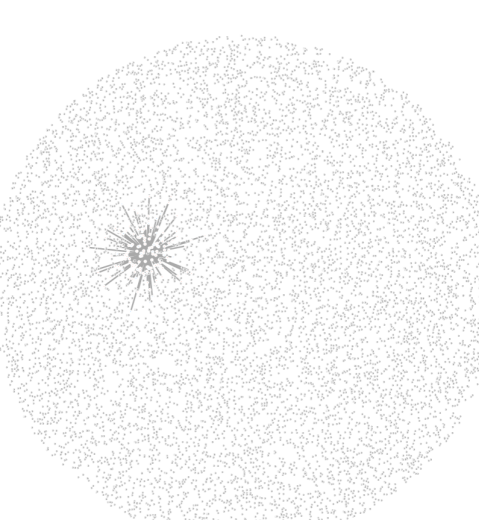
Refer to caption
Refer to caption
Figure 17: Synthesized network of 10,000 neurons; connections of only one of them are visualized. Left: excitatory connections; Right: inhibitory connections.

References

  • Aertsen et al. (1989) AM Aertsen, GL Gerstein, MK Habib, and G Palm. Dynamics of neuronal firing correlation: modulation of ”effective connectivity”. Journal of neurophysiology, 61(5):900–917, 1989.
  • Amari (1995) Shun-Ichi Amari. Information geometry of the em and em algorithms for neural networks. Neural networks, 8(9):1379–1408, 1995.
  • Arnold et al. (2007) Andrew Arnold, Yan Liu, and Naoki Abe. Temporal causal modeling with graphical granger methods. In Proceedings of the 13th ACM SIGKDD international conference on Knowledge discovery and data mining, pages 66–75. ACM, 2007.
  • Banerjee et al. (2008) Onureena Banerjee, Laurent El Ghaoui, and Alexandre d’Aspremont. Model selection through sparse maximum likelihood estimation for multivariate gaussian or binary data. Journal of machine learning research, 9(Mar):485–516, 2008.
  • Barthó et al. (2004) Peter Barthó, Hajime Hirase, Lenaïc Monconduit, Michael Zugaro, Kenneth D Harris, and György Buzsáki. Characterization of neocortical principal cells and interneurons by network interactions and extracellular features. Journal of neurophysiology, 92(1):600–608, 2004.
  • Bi and Poo (1998) Guo-qiang Bi and Mu-ming Poo. Synaptic modifications in cultured hippocampal neurons: dependence on spike timing, synaptic strength, and postsynaptic cell type. Journal of neuroscience, 18(24):10464–10472, 1998.
  • Brown et al. (2004) Emery N Brown, Robert E Kass, and Partha P Mitra. Multiple neural spike train data analysis: state-of-the-art and future challenges. Nature neuroscience, 7(5):456–461, 2004.
  • Friedman et al. (2008) Jerome Friedman, Trevor Hastie, and Robert Tibshirani. Sparse inverse covariance estimation with the graphical lasso. Biostatistics, 9(3):432–441, 2008.
  • Gerstein and Perkel (1969) George L Gerstein and Donald H Perkel. Simultaneously recorded trains of action potentials: analysis and functional interpretation. Science, 164(3881):828–830, 1969.
  • Gothard et al. (1996) Katalin M Gothard, William E Skaggs, and Bruce L McNaughton. Dynamics of mismatch correction in the hippocampal ensemble code for space: interaction between path integration and environmental cues. Journal of Neuroscience, 16(24):8027–8040, 1996.
  • Haury et al. (2012) Anne-Claire Haury, Fantine Mordelet, Paola Vera-Licona, and Jean-Philippe Vert. Tigress: trustful inference of gene regulation using stability selection. BMC systems biology, 6(1):145, 2012.
  • Hino et al. (2015) Hideitsu Hino, Ken Takano, and Noboru Murata. mmpp: A package for calculating similarity and distance metrics for simple and marked temporal point processes. R JOURNAL, 7(2):237–248, 2015.
  • Hu et al. (2015) Meng Hu, Wu Li, and Hualou Liang. A copula-based granger causality measure for the analysis of neural spike train data. IEEE/ACM Transactions on Computational Biology and Bioinformatics, 2015.
  • Hyvärinen (1999) Aapo Hyvärinen. Gaussian moments for noisy independent component analysis. IEEE Signal Processing Letters, 6(6):145–147, 1999.
  • Ito and Tsuji (2000) Hiroyuki Ito and Satoshi Tsuji. Model dependence in quantification of spike interdependence by joint peri-stimulus time histogram. Neural computation, 12(1):195–217, 2000.
  • Izhikevich (2003) Eugene M Izhikevich. Simple model of spiking neurons. IEEE Transactions on neural networks, 14(6):1569–1572, 2003.
  • Kim et al. (2011) Sanggyun Kim, David Putrino, Soumya Ghosh, and Emery N Brown. A granger causality measure for point process models of ensemble neural spiking activity. PLoS Comput Biol, 7(3):e1001110, 2011.
  • Kudrimoti et al. (1999) Hemant S Kudrimoti, Carol A Barnes, and Bruce L McNaughton. Reactivation of hippocampal cell assemblies: effects of behavioral state, experience, and eeg dynamics. Journal of Neuroscience, 19(10):4090–4101, 1999.
  • Liu et al. (2010) Han Liu, Kathryn Roeder, and Larry Wasserman. Stability approach to regularization selection (stars) for high dimensional graphical models. In Advances in neural information processing systems, pages 1432–1440, 2010.
  • Markus et al. (1994) Etan J Markus, Carol A Barnes, Bruce L McNaughton, Victoria L Gladden, and William E Skaggs. Spatial information content and reliability of hippocampal ca1 neurons: effects of visual input. Hippocampus, 4(4):410–421, 1994.
  • Nakahara and Amari (2002) Hiroyuki Nakahara and Shun-ichi Amari. Information-geometric measure for neural spikes. Neural computation, 14(10):2269–2316, 2002.
  • Nie and Tatsuno (2012) Yimin Nie and Masami Tatsuno. Information-geometric measures for estimation of connection weight under correlated inputs. Neural computation, 24(12):3213–3245, 2012.
  • Noda et al. (2014) Atsushi Noda, Hideitsu Hino, Masami Tatsuno, Shotaro Akaho, and Noboru Murata. Intrinsic graph structure estimation using graph laplacian. Neural computation, 26(7):1455–1483, 2014.
  • Perkel et al. (1967) Donald H Perkel, George L Gerstein, and George P Moore. Neuronal spike trains and stochastic point processes. 1967.
  • Quinn et al. (2011) Christopher J Quinn, Todd P Coleman, Negar Kiyavash, and Nicholas G Hatsopoulos. Estimating the directed information to infer causal relationships in ensemble neural spike train recordings. Journal of computational neuroscience, 30(1):17–44, 2011.
  • Ribeiro et al. (2004) Sidarta Ribeiro, Damien Gervasoni, Ernesto S Soares, Yi Zhou, Shih-Chieh Lin, Janaina Pantoja, Michael Lavine, and Miguel AL Nicolelis. Long-lasting novelty-induced neuronal reverberation during slow-wave sleep in multiple forebrain areas. PLoS biology, 2(1):e24, 2004.
  • Scheinberg and Rish (2009) Katya Scheinberg and Irina Rish. SINCO-a greedy coordinate ascent method for sparse inverse covariance selection problem. preprint, 2009.
  • Shimazaki et al. (2012) Hideaki Shimazaki, Shun-ichi Amari, Emery N Brown, and Sonja Grün. State-space analysis of time-varying higher-order spike correlation for multiple neural spike train data. PLoS Comput Biol, 8(3):e1002385, 2012.
  • Song et al. (2005) Sen Song, Per Jesper Sjöström, Markus Reigl, Sacha Nelson, and Dmitri B Chklovskii. Highly nonrandom features of synaptic connectivity in local cortical circuits. PLoS biology, 3(3):e68, 2005.
  • Takano et al. (2015) Ken Takano, Hideitsu Hino, Yuki Yoshikawa, and Noboru Murata. Patchworking multiple pairwise distances for learning with distance matrices. In International Conference on Latent Variable Analysis and Signal Separation, pages 287–294. Springer, 2015.
  • Tatsuno et al. (2006) Masami Tatsuno, Peter Lipa, and Bruce L McNaughton. Methodological considerations on the use of template matching to study long-lasting memory trace replay. Journal of Neuroscience, 26(42):10727–10742, 2006.
  • Tatsuno et al. (2009) Masami Tatsuno, Jean-Marc Fellous, and Shun-ichi Amari. Information-geometric measures as robust estimators of connection strengths and external inputs. Neural computation, 21(8):2309–2335, 2009.
  • Toyoizumi et al. (2009) Taro Toyoizumi, Kamiar Rahnama Rad, and Liam Paninski. Mean-field approximations for coupled populations of generalized linear model spiking neurons with markov refractoriness. Neural computation, 21(5):1203–1243, 2009.
  • Wilson and McNaughton (1994) Matthew A Wilson and Bruce L McNaughton. Reactivation of hippocampal ensemble memories during sleep. Science, 265(5172):676–679, 1994.