Membrane Paradigm and Holographic DC Conductivity for Nonlinear Electrodynamics

Abstract

Membrane paradigm is a powerful tool to study properties of black hole horizons. We first explore the properties of the nonlinear electromagnetic membrane of black holes. For a general nonlinear electrodynamics field, we show that the conductivities of the horizon usually have off-diagonal components and depend on the normal electric and magnetic fields on the horizon. Via the holographic duality, we find a model-independent expression for the holographic DC conductivities of the conserved current dual to a probe nonlinear electrodynamics field in a neutral and static black brane background. It shows that these DC conductivities only depend on the geometric and electromagnetic quantities evaluated at the horizon. We can also express the DC conductivities in terms of the temperature, charge density and magnetic field in the boundary theory, as well as the values of the couplings in the nonlinear electrodynamics at the horizon.

I Introduction

Black holes are among the most intriguing concepts of general relativity. The event horizon of a black hole is a puzzling and fascinating object, in that natural descriptions of physics often have trouble accommodating the horizon. One of the challenges of extending theories to the horizon is defining boundary conditions on the horizon. The horizon is a null hypersurface, which possesses a singular Jacobian and a both normal and tangential vector field. If one believes that $\left(1\right)$ the effective number of degrees of freedom within a few Planck lengths away from the horizon is very small, $\left(2\right)$ the interior of the black hole is a classically inaccessible region to an outside observer, an effective timelike membrane can be put just outside the horizon to have boundary conditions defined on it, instead of the horizon. These observations form the basis of the membrane paradigm for black holes.

The membrane paradigm was proposed and developed by Thorne and his Caltech colleagues in a series of papers IN-Thorn:1982mn ; IN-MacDonald:1982mn ; IN-MacDonald:1984ds ; IN-Price:1986yy ; IN-Suen:1988kq . Later, a more systematic action-based derivation was obtained by Parikh and Wilczek in IN-Parikh:1997ma , which could determine membrane properties for various field theories. The membrane paradigm was originally developed to serves as an efficient computational tool useful in dealing with some astrophysical physics in black hole backgrounds IN-Masso:1998fi ; IN-Komissarov:2004ms ; IN-Penna:2013rga . On the other hand, the membrane paradigm is also useful to study microscopic properties of black hole horizons. For example, the membrane paradigm predicts that black hole horizons are the fastest scramblers in nature IN-Susskind2005sw ; IN-Sekino:2008he . In particular, authors of IN-Fischler:2015cma studied the electromagnetic membrane properties of the horizon and considered a charged particle dropping onto the horizon in the framework of Maxwell-Chern-Simons theory. They found that black hole horizon behaved as a Hall conductor, and there were vortices introduced to the way perturbations scramble on the horizon.

The AdS/CFT duality IN-Banks:1996vh ; IN-Maldacena:1997re conjectures a connection between a strongly coupled gauge theory in $d$-dimensions on the boundary and a dual weakly coupled gravity in $\left(d+1\right)$ dimensional bulk spacetime. Recently, a renewed interest has emerged in the study of membrane paradigm in the context of the AdS/CFT duality. It has been shown that the membrane paradigm fluid on the black hole horizon is conjectured to give the low frequency limit of linear response of a strongly coupled quantum field theory at a finite temperature IN-Kovtun:2003wp ; IN-Kovtun:2004de ; IN-Iqbal:2008by ; IN-Bredberg:2010ky . In particular, identifying the currents in the boundary theory with radially independent quantities in bulk, authors of IN-Iqbal:2008by showed that the low frequency limit of the boundary theory transport coefficients could be expressed in terms of geometric quantities evaluated at the horizon. This method was later extended to calculate the DC conductivity in the presence of momentum dissipation IN-Blake:2013bqa ; IN-Donos:2014cya ; IN-Cremonini:2016avj ; IN-Bhatnagar:2017twr , where the zero mode of the current, not the current itself, did not evolve in the radial direction. Specifically, the DC thermoelectric conductivity has recently been obtained by solving a system of Stokes equations on the black hole horizon for a charged fluid in Einstein-Maxwell theory IN-Donos:2015gia . Later, the technology of IN-Donos:2015gia has been extended to various theories, e.g. Einstein-Maxwell-scalar theory IN-Banks:2015wha and including a $\theta F\wedge F$ term in the Lagrangian IN-Donos:2017mhp .

Nonlinear electrodynamics (NLED) are effective models incorporating quantum corrections to Maxwell electromagnetic theory. Among the various NLED, there are two well-known ones: $\left(1\right)$ Heisenberg–Euler effective Lagrangian that contains logarithmic terms IN-Heisenberg:1935qt . These terms describe the vacuum polarization effects and take into account one-loop quantum corrections to QED; $\left(2\right)$ Born-Infeld electrodynamics that incorporates maximal electric fields and smooths divergences of the electrostatic self-energy of point charges IN-Born:1934gh . Coupling NLED to gravity, various NLED charged black holes were derived in a number of papers IN-Soleng:1995kn ; IN-AyonBeato:1998ub ; IN-Cai:2004eh ; IN-Maeda:2008ha ; IN-Hendi:2017mgb . Some of these black holes are non–singular exact black hole solutions IN-AyonBeato:1998ub . In the framework of AdS/CFT duality, the shear viscosity was calculated in Einstein-Born-Infeld gravity IN-Cai:2008in . Holographic superconductors were studied in several NLED-gravity theory IN-Jing:2010zp ; IN-Jing:2011vz ; IN-Gangopadhyay:2012np ; IN-Roychowdhury:2012hp . In IN-Dehyadegari:2017fqo , the holographic conductivity for the black brane solutions in the massive gravity with a power-law Maxwell field was numerically investigated. A class of holographic models for Mott insulators, whose gravity dual contained NLED, was studied in IN-Baggioli:2016oju . The properties of magnetotransport in holographic Dirac-Born-Infeld models were discussed in a probe case IN-Kiritsis:2016cpm and taking into account the effects of backreaction on the geometry In-Cremonini:2017qwq .

In this paper, we will consider a neutral and static black brane background with a probe NLED field and its dual theory. The aim of the paper is to study the NLED electromagnetic membrane properties and find a model-independent expression for the holographic DC conductivities of the dual conserved current in the boundary theory. Specifically, we give a quick review of nonlinear electromagnetic fields in the curved spacetime in section II. In section III, we use the membrane paradigm to compute the conductivities of the stretched horizon. Unlike Maxwell or Maxwell-Chern-Simons theories, we find that, for a general NLED field, the conductivities would usually depend on the normal electric and magnetic fields on the stretched horizon. In section IV, we consider a charged point particle infalling into the horizon in Rindler space. It shows that effects of NLED do not affect the charge density on the stretched horizon or the scrambling time, but only could change the way the charge scramble. In section V, the DC conductivities of the dual conserved current are calculated in the framework of Gauge/Gravity duality. We show that these DC conductivities usually depend on both the geometry and values of the couplings in NLED at the black hole horizon as well as the probe charge density and magnetic field in the boundary theory. In section VI, we conclude with a brief discussion of our results. We use convention that the Minkowski metric has signature of the metric $\left(-+++\right)\,$in this paper,.

II Nonlinear Electrodynamics

In this section, we will briefly review nonlinear electromagnetic fields in the curved spacetime, mainly in order to define terms and notation and derive formulas for later use. Let us consider the action of a nonlinear electromagnetic field $A_{a}$ in a $\left(3+1\right)$-dimensional manifold $\mathcal{M}$

$$S=\int\limits_{\mathcal{M}}d^{4}x\sqrt{-g}\left[\mathcal{L}\left(s,p\right)+J^{a}A_{a}\right],$$ (1)

where we build two independent nontrivial scalars using $F_{ab}$ and none of its derivatives:

$$s =-\frac{1}{4}F^{ab}F_{ab}\text{,}$$

$$p =-\frac{1}{8}\epsilon^{abcd}F_{ab}F_{cd}\text{;}$$ (2)

the field strength is defined by $F_{ab}=\partial_{a}A_{b}-\partial_{b}A_{a}$; $\epsilon^{abcd}\equiv-\left[a\text{ }b\text{ }c\text{ }d\right]/\sqrt{-g}$ is a totally antisymmetric Lorentz tensor, and $\left[a\text{ }b\text{ }c\text{ }d\right]$ is the permutation symbol; the Lagrangian density $\mathcal{L}\left(s,p\right)$ is an arbitrary function of $s$ and $p$; $J^{a}$ is the external current. We also assume that the NLED Lagrangian would reduce to the form of Maxwell-Chern-Simons Lagrangian for small fields:

$$\mathcal{L}\left(s,p\right)\approx g\left(x\right)s+\theta\left(x\right)p,$$ (3)

where, for later convenience, we define

$$g\left(x\right)\equiv\mathcal{L}^{\left(1,0\right)}\left(0,0\right)\text{ and }\theta\left(x\right)\equiv\mathcal{L}^{\left(0,1\right)}\left(0,0\right).$$ (4)

Here we allow coordinate dependent couplings in $\mathcal{L}\left(s,p\right)$. The equations of motion obtained from the action $\left(\ref{eq:action}\right)$ are

$$\nabla_{a}G^{ab}+J^{b}=0\text{,}$$ (5)

where we define

$$G^{ab}=-\frac{\partial\mathcal{L}\left(s,p\right)}{\partial F_{ab}}=\frac{\partial\mathcal{L}\left(s,p\right)}{\partial s}F^{ab}+\frac{1}{2}\frac{\partial\mathcal{L}\left(s,p\right)}{\partial p}\epsilon^{abcd}F_{cd}.$$ (6)

Meanwhile, from the definition of $F_{ab}$, the field strength also satisfies the Bianchi identity

$$F_{\left[ab,c\right]}=\frac{1}{3}\left(F_{ab,c}+F_{bc,a}+F_{ca,b}\right)=0.$$ (7)

The electric and magnetic fields measured by an observer with $4$-velovity $U^{a}$ are given by

$$E^{a} =F^{ab}U_{b},$$

$$B^{a} =\frac{1}{2}\epsilon^{bacd}F_{cd}U_{b},$$ (8)

Note that the fields $E^{a}$ and $B^{a}$ are $3$-vectors since $E^{a}U_{a}=B^{a}U_{a}=0$. The variables $s$ and $p$ can be rewritten in terms of $E^{a}$ and $B^{a}$:

$$s =\frac{1}{2}\left(E^{a}E_{a}-B^{a}B_{a}\right),$$

$$p =-E^{a}B_{a}.$$ (9)

Similarly for $G^{ab}$, we can define auxiliary fields $D^{a}$ and $H^{a}$:

$$D^{a} =G^{ab}U_{b},$$

$$H^{a} =\frac{1}{2}\epsilon^{bacd}G_{cd}U_{b},$$ (10)

which are related to $E^{a}$ and $B^{a}$ by

$$D^{a} =\frac{\partial\mathcal{L}\left(s,p\right)}{\partial s}E^{a}-\frac{\partial\mathcal{L}\left(s,p\right)}{\partial p}B^{a},$$

$$H^{a} =\frac{\partial\mathcal{L}\left(s,p\right)}{\partial s}B^{a}+\frac{\partial\mathcal{L}\left(s,p\right)}{\partial p}E^{a}.$$ (11)

The electromagnetic $4$-current $J^{a}$ can be split into the charge density $\rho$ and current density $\mathbf{J}^{a}$ measured by the observer:

$$\rho =-J^{a}U_{a},$$

$$\mathbf{J}^{a} =J^{a}-\sigma U^{a},$$ (12)

where $\mathbf{J}^{a}$ is a 2-vector since $\mathbf{J}^{a}U_{a}=\mathbf{J}^{a}n_{a}=0$.

Born-Infeld electrodynamics is described by the Lagrangian density

$$\mathcal{L}_{\text{BI}}\left(s,p\right)=-b^{2}\sqrt{1-\frac{2s}{b^{2}}-\frac{p^{2}}{b^{4}}}+b^{2},$$ (13)

where the coupling parameter $b$ is related to the string tension $\alpha^{\prime}$ as $b=1/2\pi\alpha^{\prime}$. For small fields $s,p\ll b^{2}$, we can recover the Maxwell Lagrangian. A simple example of an electrodynamics Lagrangian with a logarithmic term has the form

$$\mathcal{L}_{\text{Log}}\left(s,p\right)=-b^{2}\log\left(1-\frac{s}{b^{2}}\right).$$ (14)

This Lagrangian also reduces to the Maxwell case in the limit $b\rightarrow\infty$.

As a simple example, let us calculate the electric and magnetic fields of a point charge in four-dimensional Minkowski space. In Minkowski space, eqns. $\left(\ref{eq:eomS}\right)$ and $\left(\ref{eq:eomB}\right)$ become

$$\nabla\times\vec{E} =-\frac{\partial\vec{B}}{\partial t}\text{,}$$

$$\nabla\cdot\vec{B} =0\text{,}$$

$$\nabla\cdot\vec{D} =\rho\text{,}$$ (15)

$$\nabla\times\vec{H} =\vec{j}+\frac{\partial\vec{D}}{\partial t}\text{,}$$

where $\rho=Q\delta^{3}\left(\vec{r}\right)$ and $\vec{j}=0$ for a point charge sitting at $\vec{r}=0$. Since $\partial\vec{E}/\partial t=\partial\vec{B}/\partial t=0$ in this case, eqns. $\left(\ref{eq:eomEB}\right)$ lead to

$$\vec{D}=\frac{Q}{4\pi r^{2}}\hat{r}\text{ and }B=0\text{.}$$ (16)

Considering $s=E^{2}/2$ and $p=0$, we can solve eqns. $\left(\ref{eq:EBDH}\right)$ for $\vec{E}$ and find that

$$\vec{E}=\frac{Q}{4\pi r^{2}}F\left(\frac{Q}{4\pi r^{2}}\right)\hat{r},$$ (17)

where $y\left(x\right)=xF\left(x\right)$ is the inverse of the function $x\left(y\right)=\mathcal{L}^{\left(1,0\right)}\left(\frac{y^{2}}{2},0\right)y$. For example, one has

$$F\left(x\right)=\left\{\begin{array}[c]{c}\frac{1}{\sqrt{1+x^{2}/b^{2}}}\text{ \ \ \ \ \ \ \ Born-Infeld electrodynamics}\\ \frac{-1+\sqrt{1+2x^{2}/b^{2}}}{x^{2}/b^{2}}\text{ \ \ \ Logarithmic electrodynamics}\end{array}\right..$$ (18)

III Membrane Paradigm

In this section, we will begin with a brief discussion of the action formulation of the black hole membrane paradigm and then examine the electromagnetic membrane in the framework of NLED. The interested reader can find a detailed discussion of the action formulation of the membrane paradigm in IN-Parikh:1997ma .

The black hole has an event horizon, $\mathcal{H}$, which is a 3-dimensional null hypersurface with a null geodesic generator $l_{a}$. We then choose a time-like surface just outside $\mathcal{H}$, which is called the stretched horizon and denoted by $\mathcal{S}$. We regard $\mathcal{S}$ as the world-tube of a family of fiducial observers, which have world lines $U^{a}$. The stretched horizon also possesses a spacelike the outward pointing normal vector $n_{a}$, which satisfies $n^{a}\nabla_{a}n^{c}=0$ on $\mathcal{S}$. Since the region inside the black hole cannot classically affect an outside observer $\mathcal{O}$, the classical equations of motion for $\mathcal{O}$ must be obtained by extremizing the action restricted to the spacetime outside the black hole, $S_{\text{out}}$. However, $S_{\text{out}}$ is not stationary on its own because there are no boundary conditions fixed at $\mathcal{H}$. To have the correct Euler-Lagrange equations, it is necessary to add a surface term $S_{\text{surf}}$ to $S_{\text{out}}$ to exactly cancel all the boundary terms. In practice, it is often more convenient to define $S_{\text{surf}}$ on $\mathcal{S}$. Consequently, the total action can be rewritten as

$$S_{\text{tot}}=\left(S_{\text{out}}+S_{\text{surf}}\right)+\left(S_{\text{in}}-S_{\text{surf}}\right),$$ (19)

where $\delta S_{\text{out}}+\delta S_{\text{surf}}=0$ will give the correct equations of motion outside $\mathcal{S}$. For the Maxwell action, the surface term can be interpreted as sources such as surface electric charges and currents IN-Parikh:1997ma .

For a nonlinear electromagnetic field $A_{a}$, the external action is given by eqn. $\left(\ref{eq:action}\right)$:

$$S_{\text{out}}=\int d^{4}x\sqrt{-g}\left[\mathcal{L}\left(s,p\right)+J^{a}A_{a}\right].$$ (20)

Integration by parts on the kinetic term of the nonlinear electromagnetic field leads to a variation at the boundary

$$-\int\limits_{\mathcal{S}}d^{3}x\sqrt{-h}n_{b}G^{ab}\delta A_{a},$$ (21)

where $h_{ab}=g_{ab}-n_{a}n_{b}$ is the induced metric on $\mathcal{S}$. To cancel this boundary contribution, we add a surface term $S_{\text{surf}}$

$$S_{\text{surf}}=\int\limits_{\mathcal{S}}d^{3}x\sqrt{\left|h\right|}j_{\text{s}}^{a}A_{a},$$ (22)

where we define the membrane current as

$$j_{\text{s}}^{a}=G^{ab}n_{b}.$$ (23)

The current $j_{\text{s}}^{a}$ is on the stretched horizon since $n_{a}j_{\text{s}}^{a}=0$. As in the Maxwell case, this surface term corresponds to the surface electric charge density $\rho=-j_{\text{s}}^{a}U_{a}$ and current density $\mathbf{j}_{\text{s}}^{a}=j_{\text{s}}^{a}-\sigma U^{a}$. From eqns. $\left(\ref{eq:eomS}\right)$, one can find a continuity equation for the membrane current $j_{\text{s}}^{a}$:

$$\nabla_{a}j_{\text{s}}^{a}=-J^{a}n_{a},$$ (24)

where $-J^{a}n_{a}$ describes the charges crossing the stretched horizon.

We now consider a general black brane background, the metric of which takes the form

$$ds^{2} =g_{ab}dx^{a}dx^{b}=g_{rr}\left(r\right)dr^{2}+g_{\mu\nu}\left(r\right)dx^{\mu}dx^{\nu}$$

$$=-g_{tt}\left(r\right)dt^{2}+g_{rr}\left(r\right)dr^{2}+g_{AB}\left(r\right)dx^{A}dx^{B}$$ (25)

$$=-g_{tt}\left(r\right)dt^{2}+g_{rr}\left(r\right)dr^{2}+g_{zz}\left(r\right)\left(dy^{2}+dz^{2}\right),$$

where indices $\left\{a,b\right\}$ run over the $\left(3+1\right)$-dimensional bulk space, $\left\{\mu,\nu\right\}$ over $3$-dimensional constant-$r$ hypersurface, and $\left\{A,B\right\}$ over spatial coordinates. We assume that there is an event horizon at $r=r_{h}$, where $g_{tt}\left(r\right)$ has a first order zero, $g_{rr}\left(r\right)$ has a first order pole, and $g_{zz}\left(r\right)$ is nonzero and finite. The Hawking temperature of the metric $\left(\ref{eq:metric}\right)$ is

$$T=\frac{\sqrt{g_{tt}^{\prime}\left(r_{h}\right)g^{rr\prime}\left(r_{h}\right)}}{4\pi}.$$ (26)

We also assume that the couplings in $\mathcal{L}\left(s,p\right)$ only depend on $r$.

Now put the stretched horizon at $r=r_{0}$ with $r_{0}-r_{h}\ll r_{h}$. This stretched horizon would have

$$n_{a}=\sqrt{g_{rr}\left(r_{0}\right)}\delta_{ar}\text{ and }U_{a}=-\sqrt{g_{tt}\left(r_{0}\right)}\delta_{at}.$$ (27)

Thus, the membrane current $\left(\ref{eq:jas}\right)$ reduces to

$$j_{\text{s}}^{\mu}=\sqrt{g_{rr}\left(r_{0}\right)}G^{\mu r}$$ (28)

To find relations among $F_{ab}\left(r_{0}\right)$, we consider a radially freely falling observer in our background. It is easy to obtain the $4$-velocity vector of this infalling observer:

$$U_{\text{FFO}}^{a}=\left(\tilde{E}g_{tt}^{-1},-\tilde{E}g_{tt}^{-1}\sqrt{\frac{g_{tt}}{g_{rr}}}\sqrt{1-\tilde{E}^{-2}g_{tt}},0,0\right),$$ (29)

where $\tilde{E}$ is the conserved energy per unit mass. The fact that $\tau$ is the proper time along the infalling world lines means that $U_{\text{FFO},a}$ is equal to the gradient of $\tau$

$$U_{\text{FFO},a}=-\partial_{\mu}\tau,$$ (30)

from which one finds

$$\frac{\partial\tau}{\partial t}=\tilde{E}\text{ and }\frac{\partial\tau}{\partial r}=\tilde{E}\sqrt{\frac{g_{rr}}{g_{tt}}}\sqrt{1-\tilde{E}^{-2}g_{tt}}.$$ (31)

Since this freely falling observer does not see the coordinate singularity at the horizon, the field strength observed by this observer must be regular. Relating $F^{\tau A}$ to $F^{rA}$ and $F^{tA}$, we obtain

$$F^{\tau A}=\frac{\partial\tau}{\partial r}F^{rA}+\frac{\partial\tau}{\partial t}F^{tA}\Longrightarrow\tilde{E}\left(\sqrt{g_{rr}}\sqrt{1-\tilde{E}^{-2}g_{tt}}F^{rA}+\sqrt{g_{tt}}F^{tA}\right)=F^{\tau A}\sqrt{g_{tt}},$$ (32)

where $F^{\tau A}$ is finite at $r=r_{h}$. On the stretched horizon, $\sqrt{g_{tt}}F^{tA}$ is the electric field measured by the fiducial observers, hence it would not go to zero as $r_{0}\rightarrow r_{h}$. Since $F^{\tau A}\sqrt{g_{tt}}\,$goes to zero as $r_{0}\rightarrow r_{h}$, eqn. $\left(\ref{eq:taoA}\right)$ leads to

$$F^{rA}\left(r_{0}\right)=-\sqrt{\frac{g_{tt}\left(r_{0}\right)}{g_{rr}\left(r_{0}\right)}}F^{tA}\left(r_{0}\right)\text{,}$$ (33)

for $r_{0}-r_{h}\ll r_{h}$.

Using eqns. $\left(\ref{eq:Gab}\right)$, $\left(\ref{eq:mur}\right)$ and $\left(\ref{eq:rt}\right)$, we find that

$$j_{\text{s}}^{A}=\mathcal{L}^{\left(1,0\right)}\left(s,p\right)|_{r=r_{0}}E^{A}-\left[A\text{ }B\right]\mathcal{L}^{\left(0,1\right)}\left(s,p\right)|_{r=r_{0}}E^{B},$$ (34)

where $\mathcal{L}^{\left(1,0\right)}\left(s,p\right)=\partial\mathcal{L}\left(s,p\right)/\partial s$ and $\mathcal{L}^{\left(0,1\right)}\left(s,p\right)=\partial\mathcal{L}\left(s,p\right)/\partial p$; the electric and magnetic fields measured by the fiducial observers on the stretched horizon are

$$E^{a}=F^{ta}\left(r_{0}\right)\sqrt{g_{tt}\left(r_{0}\right)}\text{ and }B^{a}\left(r_{0}\right)=\frac{1}{2}\frac{\left[t\text{ }a\text{ }c\text{ }d\right]}{\sqrt{g_{rr}\left(r_{0}\right)}g_{zz}\left(r_{0}\right)}F_{cd}\left(r_{0}\right)\text{, respectively;}$$

two variables $s$ and $p$ on the stretched horizon become

$$s\left(r_{0}\right)=\frac{1}{2}\left(E^{r}E_{r}-B^{r}B_{r}\right)\text{ and }p\left(r_{0}\right)=-E^{r}B_{r}.$$ (35)

Since $s$ and $p$ are scalars and the field strength observed by the freely falling observer is regular on the horizon, $s\left(r_{0}\right)$ and $p\left(r_{0}\right)$ stay finite as $r_{0}\rightarrow r_{h}$.

The conductivities of the stretched horizon can be read off from eqn. $\left(\ref{eq:mcurrent}\right)$:

$$\sigma_{\text{s}}^{yy}=\sigma_{\text{s}}^{zz}=\mathcal{L}^{\left(1,0\right)}\left(s,p\right)|_{r=r_{0}}\text{ and }\sigma_{\text{s}}^{zy}=-\sigma_{\text{s}}^{yz}=\mathcal{L}^{\left(0,1\right)}\left(s,p\right)|_{r=r_{0}},$$ (36)

where $\sigma^{zy}$ is the surface Hall conductance. In Maxwell-Chern-Simons theory with $\mathcal{L}\left(s,p\right)=s+\theta p$, one has

$$\sigma_{\text{s}}^{yy}=\sigma_{\text{s}}^{zz}=1\text{ and }\sigma_{\text{s}}^{zy}=-\sigma_{\text{s}}^{yz}=\theta,$$ (37)

which agree with what was found in IN-Fischler:2015cma . However in NLED models, the conductivities of the stretched horizon usually depend on the external fields through $s\left(r_{0}\right)$ and $p\left(r_{0}\right)$. In particular, the conductivities only depend on the normal electric and magnetic fields measured by the fiducial observers on the stretched horizon. Note that the normal components of the electric and magnetic fields in an orthonormal frame of fiducial observers are the same as in those of freely falling observers. It is noteworthy that the surface charge density $\rho_{\text{s}}$ of the stretched horizon can be related to $E_{r}$ and $B_{r}$ via

$$\rho_{\text{s}}=n_{a}D^{a}=\sqrt{g_{rr}\left(r_{0}\right)}\left[\mathcal{L}^{\left(1,0\right)}\left(s,p\right)|_{r=r_{0}}E_{r}-\mathcal{L}^{\left(0,1\right)}\left(s,p\right)|_{r=r_{0}}B_{r}\right].$$ (38)

Using this equation, we can rewrite the conductivities in terms of the surface charge density and normal magnetic field.

IV Infalling Charge in Rindler Space

In this section, we will consider dropping a charged point particle into the horizon in Rindler space. Rindler space is a good approximation to the Schwarzschild geometry in the near-horizon region $r-2M\ll 2M$ and ignores the spatial curvature there. The metric of Rindler space takes form

$$ds^{2}=-r^{2}d\omega^{2}+dr^{2}+dy^{2}+dz^{2},$$ (39)

which describes a portion of Minkowski space, namely the Rindler wedge. Minkowski coordinates $t$ and $x$ can be defined by

$$t=r\sinh\omega\text{ and }x=r\cosh\omega$$ (40)

to get the familiar Minkowski metric

$$ds^{2}=-dt^{2}+dx^{2}+dy^{2}+dz^{2}\text{.}$$ (41)

The Rindler coordinate has a coordinate singularity at $r=0$, where the determinant of the metric tensor becomes zero. In fact, there is an event horizon at $r=0$, which becomes $x=\left|t\right|$ in Minkowski coordinates and is the edge of the Rindler wedge. We will put the stretched horizon at $r=r_{0}\ll 1$, which has

$$n^{a}=\left(0,1,0,0\right)\text{ and }U^{a}=\left(r_{0}^{-1},0,0,0\right).$$ (42)

Without loss of generality, we can take a single charge to be at static at position $x=a$ in Minkowski coordinates. In the Rindler coordinates, the charge is freely falling into the horizon. In this case, the magnetic and electric fields in Minkowski coordinates have been obtained in section II and are given by eqns. $\left(\ref{eq:DB}\right)$ and $\left(\ref{eq:E}\right)$ with $r^{2}=\left(x-a\right)^{2}+y^{2}+z^{2}$, respectively. In Minkowski coordinates, the field strength is

$$F_{\text{M}}^{tx} =-F_{\text{M}}^{xt}=\frac{Q\left(x-a\right)}{4\pi\left[\left(x-a\right)^{2}+y^{2}+z^{2}\right]^{\frac{3}{2}}}F\left(\frac{Q}{4\pi\left[\left(x-a\right)^{2}+y^{2}+z^{2}\right]}\right),$$

$$F_{\text{M}}^{ty} =-F_{\text{M}}^{yt}=\frac{Qy}{4\pi\left[\left(x-a\right)^{2}+y^{2}+z^{2}\right]^{\frac{3}{2}}}F\left(\frac{Q}{4\pi\left[\left(x-a\right)^{2}+y^{2}+z^{2}\right]}\right),$$ (43)

$$F_{\text{M}}^{tz} =-F_{\text{M}}^{zt}=\frac{Qz}{4\pi\left[\left(x-a\right)^{2}+y^{2}+z^{2}\right]^{\frac{3}{2}}}F\left(\frac{Q}{4\pi\left[\left(x-a\right)^{2}+y^{2}+z^{2}\right]}\right),$$

and all the other components are zero. Performing the change of coordinates to calculate $F_{\text{R}}^{ab}$ leads to

$$j_{\text{s}}^{\omega} =\frac{Q\left(r_{0}\cosh\omega-a\right)}{4\pi r_{0}\left[\left(r_{0}\cosh\omega-a\right)^{2}+y^{2}+z^{2}\right]^{\frac{3}{2}}},$$

$$j_{\text{s}}^{\rho} =0,$$

$$j_{\text{s}}^{y} =\frac{Q}{4\pi\left[\left(r_{0}\cosh\omega-a\right)^{2}+y^{2}+z^{2}\right]^{\frac{3}{2}}}\left[y\sinh\omega-z\cosh\omega\frac{\mathcal{L}^{\left(0,1\right)}\left(s,0\right)}{\mathcal{L}^{\left(1,0\right)}\left(s,0\right)}|_{r=r_{0}}\right],$$ (44)

$$j_{\text{s}}^{z} =\frac{Q}{4\pi\left[\left(r_{0}\cosh\omega-a\right)^{2}+y^{2}+z^{2}\right]^{\frac{3}{2}}}\left[z\sinh\omega+y\cosh\omega\frac{\mathcal{L}^{\left(0,1\right)}\left(s,0\right)}{\mathcal{L}^{\left(1,0\right)}\left(s,0\right)}|_{r=r_{0}}\right]$$

where we use $F\left(X\right)\mathcal{L}^{\left(1,0\right)}\left(\frac{X^{2}}{2}F^{2}\left(X\right),0\right)=1$ to eliminate the function $F\left(X\right)$, and

$$s\left(r_{0}\right)=\frac{Q^{2}}{32\pi^{2}\left[\left(r_{0}\cosh\omega-a\right)^{2}+y^{2}+z^{2}\right]^{2}}F^{2}\left(\frac{Q}{4\pi\left[\left(r_{0}\cosh\omega-a\right)^{2}+y^{2}+z^{2}\right]}\right).$$ (45)

For Maxwell-Chern-Simons theory, we also reproduce the results in IN-Fischler:2015cma . An fiducial observer will measure a surface charge density $\rho_{\text{s}}=-j_{\text{s}}^{a}U_{a}=r_{0}j_{\text{s}}^{\omega}$. In NLED, the surface charge density $\rho_{\text{s}}$ of the stretched horizon is exactly the same as in Maxwell theory. In NLED, there is no corrections to $\rho_{\text{s}}$, but the surface currents $j_{\text{s}}^{y}$ and $j_{\text{s}}^{z}$ could receive corrections.

Let us study scrambling of a point charges on the stretched horizon for large Rindler time. When $\omega\gg 1$, we obtain

$$\rho_{\text{s}} =\frac{r_{0}Qe^{-2\omega}}{\pi\left(r_{0}^{2}+r_{\perp}^{2}\right)^{\frac{3}{2}}},$$

$$j_{\text{s}}^{y} =\frac{Q}{\pi\left(r_{0}^{2}+r_{\perp}^{2}\right)^{\frac{3}{2}}}\left[y-\frac{\theta\left(r_{0}\right)}{g\left(r_{0}\right)}z\right]$$

$$j_{\text{s}}^{z} =\frac{Q}{\pi\left(r_{0}^{2}+r_{\perp}^{2}\right)^{\frac{3}{2}}}\left[z+\frac{\theta\left(r_{0}\right)}{g\left(r_{0}\right)}y\right]$$

where $r_{\perp}^{2}=4e^{-2\omega}\left(y^{2}+z^{2}\right)$, and we use $s\left(r_{0}\right)\sim e^{-2\omega}$ in this limit. Whenever $\theta\left(r_{0}\right)\equiv\mathcal{L}^{\left(0,1\right)}\left(0,0\right)|_{r=r_{0}}\neq 0$, effects of NLED would change the way the charge scramble but not the scrambling time. In this case, there is the presence of vortices on the stretched horizon IN-Fischler:2015cma .

V DC Conductivity From Gauge/Gravity Duality

Under the long wavelength and low frequency limit, it is expected that there are connections between the near-horizon region geometry of the bulk gravity and the dual field theory living on the boundary. Observing that the currents in the boundary theory could be identified with radially independent quantities in the bulk, authors of IN-Iqbal:2008by found that the low frequency limit of linear response of the boundary theory could be determined by the membrane paradigm fluid on the stretched horizon. In particular, they derived expression for the DC conductivity of the boundary theory in terms of geometric quantities evaluated at the horizon. In IN-Iqbal:2008by , the conserved current in the boundary theory was dual to a Maxwell field in the bulk. In this section, we will follow the method in IN-Iqbal:2008by to calculate the DC conductivities of the conserved current in the boundary theory, which is dual to a NLED field in bulk.

We now consider a probe NLED field in the background of a $\left(3+1\right)$-dimensional black brane with the metric $\left(\ref{eq:metric}\right)$. For simplicity, we assume that this black brane is electrically neutral with trivial background configuration of the NLED field. This black brane describes an equilibrium state at finite temperature $T$, which is given by eqn. $\left(\ref{eq:HT}\right)$. The action of the NLED field is

$$S=\int d^{4}x\sqrt{-g}\mathcal{L}\left(s,p\right).$$ (46)

This NLED field is a U$\left(1\right)$ gauge field and dual to a conserved current $\mathcal{J}^{\mu}$ in the boundary theory. The corresponding AC conductivities are given by

$$\left\langle\mathcal{J}^{A}\left(k_{\mu}\right)\right\rangle=\sigma^{AB}\left(k_{\mu}\right)F_{Bt}\left(r_{B}\right),$$ (47)

where the boundary theory lives at $r=r_{B}\rightarrow\infty$. The DC conductivity is obtained in the long wavelength and low frequency limit:

$$\sigma^{AB}=\lim_{\omega\rightarrow 0}\lim_{\vec{k}\rightarrow 0}\sigma^{AB}\left(k_{\mu}\right).$$ (48)

Apart from varying the action, we can also derive the equations of motion using Hamiltonian formulation. Using gauge choice $A_{r}=0$, we will find the equations of motion for $A_{\mu}$ in a Hamiltonian form. From the action $\left(\ref{eq:actionN}\right)$, the conjugate momentum of the field $A_{\mu}$ with respect to $r$-foliation is given by

$$\Pi^{\mu}=\frac{\delta S}{\delta\left(\partial_{r}A_{\mu}\right)}=-\sqrt{-g}G^{r\mu},$$ (49)

where $G^{r\mu}$ are defined in eqn. $\left(\ref{eq:Gab}\right)$. Since $G^{r\mu}$ are functions of $F^{r\mu}$ and $F^{\mu\nu}$, one could solve eqn. $\left(\ref{eq:pi}\right)$ to find an expression for $F^{r\mu}$ in terms of $\Pi^{\mu}$ and $F^{\mu\nu}$:

$$F^{r\mu}=F^{r\mu}\left(\Pi^{\nu},F^{\rho\sigma}\right)\text{,}$$ (50)

where, as will be shown later, the exact form of the function $F^{r\mu}\left(\Pi^{\nu},F^{\rho\sigma}\right)$ is not important for our discussion. So the Hamiltonian is given by

$$H=\int d^{4}x\sqrt{-g}\mathcal{H}\left(\Pi^{\nu},F^{\rho\sigma}\right)=\int d^{4}x\sqrt{-g}\left[F_{r\mu}\left(\Pi^{\nu},F^{\rho\sigma}\right)\Pi^{\mu}-\mathcal{L}\left(s,p\right)\right],$$ (51)

where we use eqn. $\left(\ref{eq:Frmu}\right)$ to rewrite $s$ and $p$ in terms of $\Pi^{\nu}$ and $F^{\rho\sigma}$. Varying the Hamiltonian with respect to $A_{\mu}$, we write the equations of motion for $A_{\mu}$ in a Hamiltonian form as

$$\partial_{r}\Pi^{\mu}=-2\sqrt{-g}\partial_{\nu}\left[\frac{\partial\mathcal{H}\left(\Pi^{\eta},F^{\rho\sigma}\right)}{\partial F_{\nu\mu}}\right].$$ (52)

Moreover, the Bianchi identity gives

$$\partial_{r}F_{\mu\nu}+\partial_{\mu}F_{\nu r}\left(\Pi^{\eta},F^{\rho\sigma}\right)+\partial_{\nu}F_{r\mu}\left(\Pi^{\eta},F^{\rho\sigma}\right)=0\text{.}$$ (53)

In the long wavelength and low frequency limit, i.e. $\omega\rightarrow 0$ and $\vec{k}\rightarrow 0$ with $F^{\rho\sigma}$ and $\Pi^{\eta}$ fixed, eqns. $\left(\ref{eq:pir}\right)$ and $\left(\ref{eq:Fmunvr}\right)$ become

$$\partial_{r}\Pi^{\mu}=0\text{ and }\partial_{r}F_{\mu\nu}=0.$$ (54)

Now we discuss boundary conditions for $F_{ab}$ on the stretched horizon at $r=r_{0}\rightarrow r_{h}$ and the boundary of bulk at $r=r_{B}\rightarrow\infty$. On the stretched horizon, $s$ and $p$ become

$$s\left(r_{0}\right) =\frac{1}{2}\left[g_{rr}\left(r_{0}\right)g_{tt}\left(r_{0}\right)F^{rt}\left(r_{0}\right)^{2}-\frac{F_{yz}^{2}}{g_{zz}^{2}\left(r_{0}\right)}\right],$$

$$p\left(r_{0}\right) =\frac{g_{rr}\left(r_{0}\right)g_{tt}\left(r_{0}\right)}{\sqrt{-g\left(r_{0}\right)}}F^{rt}\left(r_{0}\right)F_{yz},$$ (55)

where we use eqn. $\left(\ref{eq:rt}\right)$ to express $F^{rA}\left(r_{0}\right)$ in terms of $F^{tA}\left(r_{0}\right)$, and $F_{yz}$ is an $r$-independent quantity. Using eqns. $\left(\ref{eq:mur}\right)$ and $\left(\ref{eq:pi}\right)$, one can relate $\Pi^{A}\left(r_{0}\right)$ to $j_{\text{s}}^{A}$:

$$\Pi^{A}\left(r_{0}\right)=\sqrt{g_{tt}\left(r_{0}\right)}g_{zz}\left(r_{0}\right)j_{s}^{A}=\mathcal{L}^{\left(1,0\right)}\left(s,p\right)|_{r=r_{0}}F_{At}-\left[A\text{ }B\right]\mathcal{L}^{\left(0,1\right)}\left(s,p\right)|_{r=r_{0}}F_{Bt},$$ (56)

where $F_{At}$ is also $r$-independent. On the boundary of bulk, it showed in IN-Iqbal:2008by ; DCFGGD-Hartnoll:2009sz that one point function of $\mathcal{J}^{A}$ in the presence of source $F_{\mu v}$ can be written as

$$\left\langle\mathcal{J}^{\mu}\right\rangle=\Pi^{\mu}\left(r_{B}\right).$$ (57)

Since $\Pi^{A}$ and $F_{At}$ are $r$-independent in zero momentum limit, we can use eqns. $\left(\ref{eq:piI0}\right)$ and $\left(\ref{eq:Jpi}\right)$ to show that

$$\left\langle\mathcal{J}^{A}\left(k_{\mu}\rightarrow 0\right)\right\rangle=\mathcal{L}^{\left(1,0\right)}\left(s,p\right)|_{r=r_{0}}F_{At}\left(k_{\mu}\rightarrow 0\right)-\left[A\text{ }B\right]\mathcal{L}^{\left(0,1\right)}\left(s,p\right)|_{r=r_{0}}F_{Bt}\left(k_{\mu}\rightarrow 0\right).$$ (58)

Comparing eqn. $\left(\ref{eq:sigma}\right)$ with eqn. $\left(\ref{eq;J}\right)$, we can read off the DC conductivities in the dual theory:

$$\sigma^{yy}=\sigma^{zz}=\mathcal{L}^{\left(1,0\right)}\left(s,p\right)|_{r=r_{h}}\text{ and }\sigma^{zy}=-\sigma^{yz}=\mathcal{L}^{\left(0,1\right)}\left(s,p\right)|_{r=r_{h}},$$ (59)

where we take the limit $r\rightarrow r_{h}$. Note that the DC conductivity in NLED just with $s$ was also obtained in IN-Baggioli:2016oju , where their eqn. $\left(31\right)$ in the probe case agrees with our expression for $\sigma^{yy}$ in eqns. $\left(\ref{eq:Conrh}\right)$.

To express $F^{rt}\left(r_{h}\right)$ in terms of quantities in the boundary theory, we can use the following formula

$$\Pi^{t}\left(r_{h}\right)=\Pi^{t}\left(r\rightarrow\infty\right)=\left\langle\mathcal{J}^{0}\right\rangle=\rho,$$ (60)

where $\rho$ can be interpreted as the charge density in the dual field theory. Eqn. $\left(\ref{eq:rho}\right)$ becomes

$$\sqrt{\eta}g_{zz}\left(r_{h}\right)\mathcal{L}^{\left(1,0\right)}\left(s,p\right)|_{r=r_{h}}F^{rt}\left(r_{h}\right)+\mathcal{L}^{\left(0,1\right)}\left(s,p\right)|_{r=r_{h}}F_{yz}=-\rho,$$ (61)

where eqns. $\left(\ref{eq:sp}\right)$ give

$$s\left(r_{h}\right) =\frac{1}{2}\left[\eta F^{rt}\left(r_{h}\right)^{2}-\frac{F_{yz}^{2}}{g_{zz}^{2}\left(r_{h}\right)}\right],$$

$$p\left(r_{h}\right) =\frac{\sqrt{\eta}}{g_{zz}\left(r_{h}\right)}F^{rt}\left(r_{h}\right)F_{yz}.$$ (62)

One could solve eqn. $\left(\ref{eq:rhoF}\right)$ to express $F^{rt}\left(r_{h}\right)$ in terms of $\rho$ and $F_{yz}$ and the plug this expression into eqn. $\left(\ref{eq:Conrh}\right)$ to write $\sigma^{AB}$ in terms of $\rho$ and $F_{yz}$. Note $F_{yz}$ can be treated as the magnetic field in the $\left(2+1\right)$ dimensional boundary theory, in which the magnetic field is a scalar filed. .

Let us consider $\sigma^{AB}$ in Born-Infeld and Logarithmic electrodynamics discussed above. We find that for Born-Infeld electrodynamics,

$$\sigma^{yy}=\sigma^{zz}=\frac{\sqrt{1+F_{yz}^{2}/\left[b^{2}g_{zz}^{2}\left(r_{h}\right)\right]+\rho^{2}/\left[b^{2}g_{zz}^{2}\left(r_{h}\right)\right]}}{1+F_{yz}^{2}/\left[b^{2}g_{zz}^{2}\left(r_{h}\right)\right]},$$

$$\sigma^{yz}=-\sigma^{zy}=\frac{\rho F_{yz}/\left[b^{2}g_{zz}^{2}\left(r_{h}\right)\right]}{1+F_{yz}^{2}/\left[b^{2}g_{zz}^{2}\left(r_{h}\right)\right]},$$ (63)

and for Logarithmic electrodynamics

$$\sigma^{yy}=\sigma^{zz}=\frac{1+\sqrt{1+\left\{2+F_{yz}^{2}/\left[b^{2}g_{zz}^{2}\left(r_{h}\right)\right]\right\}\rho^{2}/\left[g_{zz}^{2}\left(r_{h}\right)b^{2}\right]}}{2+F_{yz}^{2}/\left[b^{2}g_{zz}^{2}\left(r_{h}\right)\right]},$$

$$\sigma^{zy}=-\sigma^{yz}=0.$$ (64)

Note that the DC conductivity matrix of a holographic Dirac-Born-Infeld model in the probe limit has been calculated in IN-Kiritsis:2016cpm . The eqns. $\left(3.1\right)$ and $\left(3.2\right)$ with $S=0$ in IN-Kiritsis:2016cpm turn out to be the same as our results $\left(\ref{eq:sigmaB}\right)$. In FIG. 1, we plot the DC conductivities versus $\rho$ and $F_{yz}$, of the conserved current dual to the bulk electromagnetic field in both Born-Infeld and Logarithmic electrodynamics. The parameter $b^{2}g_{zz}^{2}\left(r_{h}\right)$ sets a scale in the dual field theory. When $\rho^{2},F_{yz}^{2}\ll b^{2}g_{zz}^{2}\left(r_{h}\right)$, we practically reproduce the results for Maxwell theory. On the other hand, effects of nonlinearity of the electromagnetic fields start to play an important role when $\rho^{2}$ or $F_{yz}^{2}$ are around the scale $b^{2}g_{zz}^{2}\left(r_{h}\right)$. At zero charge density, the diagonal components of the DC conductivities in both Born-Infeld and Logarithmic electrodynamics are non-zero. These non-zero values can be interpreted as incoherent contributions DCFGGD-Davison:2015bea , known as the charge conjugation symmetric terms, which are independent of the charge density $\rho$. As shown in FIG. 1, the diagonal DC conductivity $\sigma^{yy}$ increases with increasing $\left|\rho\right|$ at constant $F_{yz}$, which is a feature similar to the Drude metal. For the Drude metal, a larger charge density provides more available mobile charge carriers to efficiently transport charge. At constant $\rho$, $\sigma^{yy}$ decreases with increasing $\left|F_{yz}\right|$, which means a positive magneto-resistance.

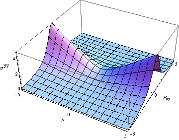
(a) Plot of $\sigma^{yy}$ against $\rho$ and $F_{yz}$ for Born-Infeld electrodynamics

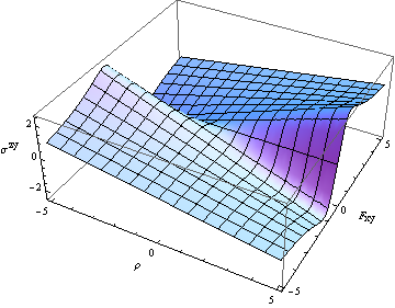
(b) Plot of $\sigma^{yz}$ against $\rho$ and $F_{yz}$ for Born-Infeld electrodynamics

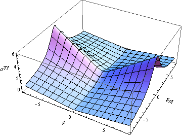
(c) Plot of $\sigma^{yy}$ against $\rho$ and $F_{yz}$ for Logarithmic electrodynamics

Figure 1: Plots of the DC conductivities of the conserved current dual to the bulk electromagnetic field in Born-Infeld and Logarithmic electrodynamics. Here we set $b^{2}g_{zz}^{2}\left(r_{h}\right)=1$.

Since $r_{h}$ is related to the Hawking temperature $T$ by eqn. $\left(\ref{eq:HT}\right)$, we can now discuss the temperature dependence of the conductivities. For simplicity and concreteness, we consider the Schwarzschild AdS black brane

$$ds^{2}=-\left(r^{2}-r_{h}^{3}/r\right)dt^{2}+\frac{dr^{2}}{\left(r^{2}-r_{h}^{3}/r\right)}+r^{2}\left(dy^{2}+dz^{2}\right),$$ (65)

where we take the AdS radius $L=1$, and $r_{h}$ determines the Hawking temperature of the black brane:

$$T=\frac{3r_{h}}{4\pi}\text{.}$$ (66)

Therefore, we obtain that for Born-Infeld electrodynamics,

$$\sigma^{yy} =\sigma^{zz}=\frac{\sqrt{1+\lambda F_{yz}^{2}/T^{4}+\lambda\rho^{2}/T^{4}}}{\lambda F_{yz}^{2}/T^{4}+1}$$ (67)

$$\sigma^{yz} =-\sigma^{zy}=\frac{\lambda\rho F_{yz}/T^{4}}{1+\lambda F_{yz}^{2}/T^{4}},$$ (68)

and for Logarithmic electrodynamics

$$\sigma^{yy}=\sigma^{zz}=\frac{1+\sqrt{1+\left(2+\lambda F_{yz}^{2}/T^{4}\right)\lambda\rho^{2}/T^{4}}}{2+\lambda F_{yz}^{2}/T^{4}},$$ (69)

where $\lambda\equiv b^{-2}\left(4\pi/3\right)^{-4}$ is a parameter associated with the conserved current $\mathcal{J}^{\mu}$ in the boundary theory. In the high temperature limit, we would recover the results for Maxwell theory. When $T^{4}\ll\rho^{2}/b^{2}$ and $F_{yz}^{2}/b^{2}$, the low temperature behavior of $\sigma^{AB}$ is

$$\sigma^{yy}=\sigma^{zz}\sim T^{2}\text{ and }\sigma^{zy}=-\sigma^{yz}\sim T^{0}\text{ for Born-Infeld electrodynamics,}$$ (70)

and

$$\sigma^{yy}=\sigma^{zz}\sim T^{0}\text{ for Logarithmic electrodynamics.}$$ (71)

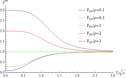
Figure 2: Plot of $\rho^{yy}$ versus $T/\sqrt{\rho}$ in Logarithmic electrodynamics.

One can define a metal and an insulator for $d\rho^{yy}/dt>0$ and $d\rho^{yy}/dt<0$, respectively, where the resistivity matrix $\left\{\rho^{AB}\right\}$ is the inverse of the conductivity matrix $\left\{\sigma^{AB}\right\}$. The metal-insulator transition in Born-Infeld electrodynamics has been discussed in In-Cremonini:2017qwq . So we here focus on Logarithmic electrodynamics. In FIG. 2, we plot $\rho^{yy}$ versus $T/\sqrt{\rho}$ for various values of $F_{yz}/\sqrt{\rho}$. The temperature dependence of $\rho^{yy}$ is similar to the case with a larger value of the momentum dissipation parameter in In-Cremonini:2017qwq . One has an insulator phase for $F_{yz}<\rho$ and a metal one for $F_{yz}>\rho$. A metal-insulator transition could occur at $F_{yz}=\rho$, where $\rho^{yy}=1$ is independent of the temperature.

VI Discussion and Conclusion

In the first part of this paper, we have used the membrane paradigm to study the electromagnetic membrane of black holes in NLED. In the membrane paradigm, the stretched horizon is regarded as a boundary hypersurface with the surface charge and current, which terminate the normal $D$ and tangential $H$ fields in the region exterior to the horizon, and annul them in the interior region. For Maxwell theory, it is well known that the horizon can be interpreted as an ohmic conductor with a constant resistivity. It showed in IN-Fischler:2015cma that the horizon behaved as a Hall conductor with surface Hall conductance in Maxwell-Chern-Simons theory. We derived the conductivities of the surface current for a general NLED and found that the conductivities usually depended on the normal electric and magnetic fields on the stretched horizon. We also showed that there was Hall conductance for the stretched horizon when $\mathcal{L}^{\left(0,1\right)}\left(s,p\right)$ was not zero on the horizon.

To study effects of NLED on charges scrambling on the stretched horizon, we considered a simple scenario, in which a charged point particle freely falls into the horizon in Rindler space. Our results showed that, during the free falling, the surface charge density in NLED was the same as in Maxwell theory. However, the effects of NLED would play a role in the surface current density. In particular, when $\mathcal{L}^{\left(0,1\right)}\left(s,p\right)$ did not vanish on the horizon, there would be presence of vortices. In the late time limit, NLED would not change the scrambling time. This is expected since electric field becomes smaller and smaller in this limit, and we assume that NLED would reduce to Maxwell-Chern-Simons theory for small fields. In IN-Fischler:2015cma , it was found that $\theta$-term only changed the way the charge scramble but not the scrambling time in Maxwell-Chern-Simons theory. If some NLED differs from Maxwell-Chern-Simons theory in IR limit, one would expect the scrambling time might be changed in this NLED.

In the second part of this paper, we used the membrane paradigm approach of IN-Iqbal:2008by to calculate DC conductivities of an conserved current in a field theory living on the boundary of some black brane. We assumed the this conserved current was dual to a probe NLED field in bulk. We found that the conjugate momentum of the NLED field encoded the information about the conductivities both on the stretched horizon and in the boundary theory and, in the zero frequency limit, did not evolve in the radial direction. Therefore, we showed that these DC conductivities depended only on the geometry and NLED fields at the black hole horizon, not on these of the whole bulk geometry. Relating electromagnetic quantities at the horizon to these in the boundary theory, we also showed that the DC conductivities usually depended on the probe charge density and magnetic field in the boundary theory.

We conclude this paper with a few remarks. First, we showed that the DC conductivities depended on the values of the couplings in NLED at the horizon. However, authors of IN-Iqbal:2008by showed, in Maxwell-Chern-Simons theory, the Hall conductivity $\sigma^{yz}$ was determined by the value of $\theta$ coupling at the boundary of the bulk. We think that the discrepancy comes from that authors of IN-Iqbal:2008by failed to realize that the first term on the left-hand side of eqn. $\left(53\right)$ in IN-Iqbal:2008by was not $r$-independent any more in Maxwell-Chern-Simons theory. On the stretched horizon, this term only contributes to the diagonal components of the conductivities. However, this term is now $r$-dependent and would contribute to the off-diagonal components as well as the diagonal ones on the boundary of bulk. In other words, the Hall conductivity of the boundary theory receives contributions from both terms on the left-hand side of eqn. $\left(53\right)$, not just the first one. These two contributions indeed make the Hall conductivity depend on the value of $\theta$ coupling at the horizon. This incorrect statement of IN-Iqbal:2008by has also been noted in IN-Donos:2017mhp , where the authors found that the $\theta$ parameter could vanish on the boundary with non-vanishing values on the horizon, hence giving rise to non-vanishing Hall conductivity.

Second, one usually only turns on the electric field in the boundary theory to calculate the holographic conductivities due to difficulties of solving the differential equations. On the other hand, membrane paradigm provides a simple way to obtain the dependence of holographic DC conductivities on the electromagnetic quantities in the boundary theory, e.g. the charge density and magnetic field. Our analysis was carried out in the long wavelength and low frequency limit, which corresponds to an equilibrium and homogeneous state. In particular, the charge density and magnetic field in the boundary theory are kept fixed, time independent and homogeneous in this limit.

Finally, we only considered a neutral black brane, which is dual to a boundary theory without a background charge density. As shown in IN-Blake:2013bqa , the low frequency behavior of the conductivities depends crucially on whether there is a background charge density. It is very interesting to study the behavior of DC conductivities in a boundary theory with a non-vanishing background charge density, which is dual to a NLED charged black hole.

- (1) K. S. Thorne and D. MacDonald, “Electrodynamics in curved spacetime: 3 + 1 formulation,” Mon. Not. Roy. Astron. Soc. 198, 339 (1982). doi:10.1093/mnras/198.2.339
- (2) D. MacDonald and K. S. Thorne, “Black-hole electrodynamics: an absolute-space/universal-time formulation,” Mon. Not. Roy. Astron. Soc. 198, 345 (1982). doi:10.1093/mnras/198.2.345
- (3) D. MacDonald and W. M. Suen, “Membrane viewpoint on black holes: Dynamical electromagnetic fields near the horizon,” Phys. Rev. D 32, 828 (1984). doi:10.1103/PhysRevD.32.848
- (4) R. H. Price and K. S. Thorne, “Membrane Viewpoint on Black Holes: Properties and Evolution of the Stretched Horizon,” Phys. Rev. D 33, 915 (1986). doi:10.1103/PhysRevD.33.915
- (5) W. M. Suen, R. H. Price and I. H. Redmount, “Membrane Viewpoint on Black Holes: Gravitational Perturbations of the Horizon,” Phys. Rev. D 37, 2761 (1988). doi:10.1103/PhysRevD.37.2761
- (6) M. Parikh and F. Wilczek, “An Action for black hole membranes,” Phys. Rev. D 58, 064011 (1998) doi:10.1103/PhysRevD.58.064011 [gr-qc/9712077].
- (7) J. Masso, E. Seidel, W. M. Suen and P. Walker, “Event horizons in numerical relativity 2.: Analyzing the horizon,” Phys. Rev. D 59, 064015 (1999) doi:10.1103/PhysRevD.59.064015 [gr-qc/9804059].
- (8) S. S. Komissarov, “Electrodynamics of black hole magnetospheres,” Mon. Not. Roy. Astron. Soc. 350, 407 (2004) doi:10.1111/j.1365-2966.2004.07446.x [astro-ph/0402403].
- (9) R. F. Penna, R. Narayan and A. Sadowski, “General Relativistic Magnetohydrodynamic Simulations of Blandford-Znajek Jets and the Membrane Paradigm,” Mon. Not. Roy. Astron. Soc. 436, 3741 (2013) doi:10.1093/mnras/stt1860 [arXiv:1307.4752 [astro-ph.HE]].
- (10) L. Susskind and J. S. Lindesay, Black Holes, Information, and the String Theory Revolution: The Holographic Universe (Singapore, World Scientific, 2005).
- (11) Y. Sekino and L. Susskind, “Fast Scramblers,” JHEP 0810, 065 (2008) doi:10.1088/1126-6708/2008/10/065 [arXiv:0808.2096 [hep-th]].
- (12) W. Fischler and S. Kundu, “Hall Scrambling on Black Hole Horizons,” Phys. Rev. D 92, no. 4, 046008 (2015) doi:10.1103/PhysRevD.92.046008 [arXiv:1501.01316 [hep-th]].
- (13) T. Banks, W. Fischler, S. H. Shenker and L. Susskind, “M theory as a matrix model: A Conjecture,” Phys. Rev. D 55, 5112 (1997) doi:10.1103/PhysRevD.55.5112 [hep-th/9610043].
- (14) J. M. Maldacena, “The Large N limit of superconformal field theories and supergravity,” Int. J. Theor. Phys. 38, 1113 (1999) [Adv. Theor. Math. Phys. 2, 231 (1998)] doi:10.1023/A:1026654312961 [hep-th/9711200].
- (15) P. Kovtun, D. T. Son and A. O. Starinets, “Holography and hydrodynamics: Diffusion on stretched horizons,” JHEP 0310, 064 (2003) doi:10.1088/1126-6708/2003/10/064 [hep-th/0309213].
- (16) P. Kovtun, D. T. Son and A. O. Starinets, “Viscosity in strongly interacting quantum field theories from black hole physics,” Phys. Rev. Lett. 94, 111601 (2005) doi:10.1103/PhysRevLett.94.111601 [hep-th/0405231].
- (17) N. Iqbal and H. Liu, “Universality of the hydrodynamic limit in AdS/CFT and the membrane paradigm,” Phys. Rev. D 79, 025023 (2009) doi:10.1103/PhysRevD.79.025023 [arXiv:0809.3808 [hep-th]].
- (18) I. Bredberg, C. Keeler, V. Lysov and A. Strominger, “Wilsonian Approach to Fluid/Gravity Duality,” JHEP 1103, 141 (2011) doi:10.1007/JHEP03(2011)141 [arXiv:1006.1902 [hep-th]].
- (19) M. Blake and D. Tong, “Universal Resistivity from Holographic Massive Gravity,” Phys. Rev. D 88, no. 10, 106004 (2013) doi:10.1103/PhysRevD.88.106004 [arXiv:1308.4970 [hep-th]].
- (20) A. Donos and J. P. Gauntlett, “Thermoelectric DC conductivities from black hole horizons,” JHEP 1411, 081 (2014) doi:10.1007/JHEP11(2014)081 [arXiv:1406.4742 [hep-th]].
- (21) S. Cremonini, H. S. Liu, H. Lu and C. N. Pope, “DC Conductivities from Non-Relativistic Scaling Geometries with Momentum Dissipation,” JHEP 1704, 009 (2017) doi:10.1007/JHEP04(2017)009 [arXiv:1608.04394 [hep-th]].
- (22) N. Bhatnagar and S. Siwach, “DC conductivity with external magnetic field in hyperscaling violating geometry,” arXiv:1707.04013 [hep-th].
- (23) A. Donos and J. P. Gauntlett, “Navier-Stokes Equations on Black Hole Horizons and DC Thermoelectric Conductivity,” Phys. Rev. D 92, no. 12, 121901 (2015) doi:10.1103/PhysRevD.92.121901 [arXiv:1506.01360 [hep-th]].
- (24) E. Banks, A. Donos and J. P. Gauntlett, “Thermoelectric DC conductivities and Stokes flows on black hole horizons,” JHEP 1510, 103 (2015) doi:10.1007/JHEP10(2015)103 [arXiv:1507.00234 [hep-th]].
- (25) A. Donos, J. P. Gauntlett, T. Griffin, N. Lohitsiri and L. Melgar, “Holographic DC conductivity and Onsager relations,” JHEP 1707, 006 (2017) doi:10.1007/JHEP07(2017)006 [arXiv:1704.05141 [hep-th]].
- (26) W. Heisenberg and H. Euler, “Consequences of Dirac’s theory of positrons,” Z. Phys. 98, 714 (1936) doi:10.1007/BF01343663 [physics/0605038].
- (27) M. Born and L. Infeld, “Foundations of the new field theory,” Proc. Roy. Soc. Lond. A 144, 425 (1934). doi:10.1098/rspa.1934.0059
- (28) H. H. Soleng, “Charged black points in general relativity coupled to the logarithmic U(1) gauge theory,” Phys. Rev. D 52, 6178 (1995) doi:10.1103/PhysRevD.52.6178 [hep-th/9509033].
- (29) E. Ayon-Beato and A. Garcia, “Regular black hole in general relativity coupled to nonlinear electrodynamics,” Phys. Rev. Lett. 80, 5056 (1998) doi:10.1103/PhysRevLett.80.5056 [gr-qc/9911046].
- (30) R. G. Cai, D. W. Pang and A. Wang, “Born-Infeld black holes in (A)dS spaces,” Phys. Rev. D 70, 124034 (2004) doi:10.1103/PhysRevD.70.124034 [hep-th/0410158].
- (31) H. Maeda, M. Hassaine and C. Martinez, “Lovelock black holes with a nonlinear Maxwell field,” Phys. Rev. D 79, 044012 (2009) doi:10.1103/PhysRevD.79.044012 [arXiv:0812.2038 [gr-qc]].
- (32) S. H. Hendi, B. Eslam Panah, S. Panahiyan and A. Sheykhi, “Dilatonic BTZ black holes with power-law field,” Phys. Lett. B 767, 214 (2017) doi:10.1016/j.physletb.2017.01.066 [arXiv:1703.03403 [gr-qc]].
- (33) R. G. Cai and Y. W. Sun, “Shear Viscosity from AdS Born-Infeld Black Holes,” JHEP 0809, 115 (2008) doi:10.1088/1126-6708/2008/09/115 [arXiv:0807.2377 [hep-th]].
- (34) J. Jing and S. Chen, “Holographic superconductors in the Born-Infeld electrodynamics,” Phys. Lett. B 686, 68 (2010) doi:10.1016/j.physletb.2010.02.022 [arXiv:1001.4227 [gr-qc]].
- (35) J. Jing, Q. Pan and S. Chen, “Holographic Superconductors with Power-Maxwell field,” JHEP 1111, 045 (2011) doi:10.1007/JHEP11(2011)045 [arXiv:1106.5181 [hep-th]].
- (36) S. Gangopadhyay and D. Roychowdhury, “Analytic study of Gauss-Bonnet holographic superconductors in Born-Infeld electrodynamics,” JHEP 1205, 156 (2012) doi:10.1007/JHEP05(2012)156 [arXiv:1204.0673 [hep-th]].
- (37) D. Roychowdhury, “Effect of external magnetic field on holographic superconductors in presence of nonlinear corrections,” Phys. Rev. D 86, 106009 (2012) doi:10.1103/PhysRevD.86.106009 [arXiv:1211.0904 [hep-th]].
- (38) A. Dehyadegari, M. Kord Zangeneh and A. Sheykhi, “Holographic conductivity in the massive gravity with power-law Maxwell field,” Phys. Lett. B 773, 344 (2017) doi:10.1016/j.physletb.2017.08.029 [arXiv:1703.00975 [hep-th]].
- (39) M. Baggioli and O. Pujolas, “On Effective Holographic Mott Insulators,” JHEP 1612, 107 (2016) doi:10.1007/JHEP12(2016)107 [arXiv:1604.08915 [hep-th]].
- (40) E. Kiritsis and L. Li, “Quantum Criticality and DBI Magneto-resistance,” J. Phys. A 50, no. 11, 115402 (2017) doi:10.1088/1751-8121/aa59c6 [arXiv:1608.02598 [cond-mat.str-el]].
- (41) S. Cremonini, A. Hoover and L. Li, “Backreacted DBI Magnetotransport with Momentum Dissipation,” JHEP 1710, 133 (2017) doi:10.1007/JHEP10(2017)133 [arXiv:1707.01505 [hep-th]].
- (42) S. A. Hartnoll, “Lectures on holographic methods for condensed matter physics,” Class. Quant. Grav. 26, 224002 (2009) doi:10.1088/0264-9381/26/22/224002 [arXiv:0903.3246 [hep-th]].
- (43) R. A. Davison and B. Goutéraux, “Dissecting holographic conductivities,” JHEP 1509, 090 (2015) doi:10.1007/JHEP09(2015)090 [arXiv:1505.05092 [hep-th]].