Routing surface plasmons by a quantum-dot nanostructure: nonlinear dispersion effects

Abstract

Usually, the liner waveguides with single quantum emitters are utilized as routers to construct the quantum network in quantum information processings. Here, we investigate the influence of the nonlinear dispersion on quantum routing of single surface plasmons, between two metal nanowires with a pair of quantum dots. By using a full quantum theory in real space, we obtain the routing probabilities of a single surface plasmon into the four outports of two plasmonic waveguides scattered by a pair of quantum dots. It is shown that, by properly designing the inter-dot distance and the dot-plasmon couplings, the routing capability of the surface plasmons between the plasmonic waveguide channels can be significantly higher than the relevant network formed by the single-emitter waveguides with the linear dispersions. Interestingly, the present quadratic dispersions in the waveguides deliver the manifest Fano-like resonances of the surface-plasmon transport. Therefore, the proposed double-dot configuration could be utilized as a robust quantum router for controlling the surface-plasmon routing in the plasmonic waveguides and a plasmonic Fano-like resonance controller.

PACS numbers: 42.50.Ex, 03.65.Nk, 73.20.Mf, 73.21.La

Quantum nodes are the key elements of the quantum network Kimble , since they coherently connect different quantum channels of the network. Quantum routers in the nodes, provided usually by these systems of waveguides and quantum emitters, are utilized to control the propagating paths of the quantum signals, wherein the photons are served as the ideal carriers of the information in these quantum channels, due to their long-lived coherences and less dissipations Brien .

Recently, many theoretical Zhou ; Lu ; Yan ; Agarwal ; Xia ; Lemr ; wei2 ; wei3 ; Lu2 and experimental Aoki ; Hoi ; Shomroni investigations have been devoted to the quantum routings of single photons in various optical quantum networks. Typically, Zhou et al and Lu et al demonstrated how to realize the quantum routing of a single photon in the X-shaped coupled-resonator waveguides by using the scattering of a three-level atom. It showed that, with the help of a classical driving Zhou ; Lu , single photons incident from one channel can be transferred into another one. Based on the photonic interferences related to the different phases acquired in different paths, Yan et al Yan examined that single-photon routing can be realized in a network with multiple input and output ports. However, low routing rate (no more than 0.5) of the single photons from the input channel into another channel exists in these single-emitter configurations, due to the emission asymmetry of the quantum emitter, which may restrict its more potential applications. For a multichannel quantum network, it is thus of considerable interest to design a quantum router with high routing capability.

Surface plasmons(SPs), known as the collective excitations of the electrons on metal-dielectric interfaces, play an important role in confining the electromagnetic wave at a nanometer scale, as the important information carriers in various functional nanophotonic devices and integrated optical systems Tame . Additionally, SPs provide many potential applications in quantum computation and quantum information processing, since they reveal strong analogies to the photons propagating along the conventional dielectric optical components Zia ; Yu ; Savel . With the recent experimental developments, an integrated system of a single metal nanowire coupled with quantum dots (QDs) has been fabricated successfully as a plasmonic waveguide Akimov ; Fedutik , which provides an idea platform to investigate the coherent transport of the SPs. Consequently, wide attention has been addressed to the transport properties of the SPs coupled to the waveguides in the linear dispersion regime, and transistors Chang ; Hong , switching Kim1 , and scattering grating Li devices of SPs have been designed accordingly. Within such a device, the Fano resonance Chen1 ; Chen2 ; Cheng1 and photonic entanglements Chen3 ; Chen4 have also been demonstrated. However, the transport of the SPs with nonlinear dispersion relations has been paid relatively-less attention, although certain interesting behaviors, e.g., the four-peak structure in the reflected spectrum Cheng3 , jiggling scattering behavior, and Fano-like resonance have been predicted Chen5 .

Motivated by the work mentioned above, we discuss how to implement the high-efficient quantum routing of the SPs in a nonlinear waveguide, which is made of two metal nanowires coupled to two separated QDs. The simple quantum network model, with two SPs channels and four ports, is served as a quantum router of the SPs inputting from one of the ports. By adopting a full quantum theory in real space, the reflection and transmission probabilities of single SPs into four ports are obtained exactly. It has shown that, due to the quadratic dispersions in the double-dot configuration, the routing capability of single SPs transferred from the incident channel into another channel can reach to an extremely-high value, by properly designing the inter-dot distance and the QD-SP couplings. Furthermore, the jiggling behavior and multiple Fano-like shapes of the scattering spectra can be observed. This implies that the proposed system may be served as a robust quantum router and a Fano-like resonance controller of the SPs for various integrated quantum optical applications.

I Theoretical mode and its exact solution

As shown in Fig. 1, the considered system consists of two two-level QDs separated by a distance $d$, which are coupled to two one-dimensional metal nanowires. The QD-1(2) is characterized by the ground state $|g_{1(2)}\rangle$ and excited state $|e_{1(2)}\rangle$. The two nanowires are connected by the two distant QDs with the coupling strength $V_{nm}$($n=1,2;m=a,b$ throughout the paper) between nanowire SPs and QDs. For the dispersion relations of nanowire SPs, we focus on the nonlinear case, which exhibits a parabola-like curve with a local minimum for the $1$th excitation mode Chen8 ; Chen9 . In the parabola-like frequency diagram, the dispersion relation $\omega_{k}$ around the local minimum can be approximated as a quadratic form as follows:

$$\omega_{k}=E_{k}/\hbar=\omega_{c}+A(k-k_{0})^{2},$$ (1)

where $k$ is the wavevector of SP and $k_{0}$ is the wavevector for the local minimum frequency $\omega_{c}$. Adopting the units in Ref Chang2 , the value of $A$ is about $0.0001$, and the value of the reduced wavevector $K_{0}(=k_{0}c/\omega_{p})$ around the local minimum is about 15, where $\hbar\omega_{p}=3.76eV$ is the plasma energy of the silver nanowire. For simplicity, we assume that the two nanowires are identical and have the same frequency $\omega_{c}$ and the same value of $A$. When a single SP is incident from the left of the nanowire-a, it will propagate or be reflected by the QDs along the four ports of the two nanowire channels, as the system is served as a quantum router.

The real-space Hamiltonian Chen5 ; Shen describing the system is expressed as follows:

$$H/\hbar=\sum_{m=a,b}\int dx{\bigg{\{}}(\omega_{c}+Ak_{0}^{2})[C_{Rm}^{{\dagger}}(x)C_{Rm}(x)$$

$$+C_{Lm}^{{\dagger}}(x)C_{Lm}(x)]$$

$$-2Ak_{0}[-iC_{Rm}^{{\dagger}}(x)\frac{\partial}{\partial x}C_{Rm}(x)+iC_{Lm}^{{\dagger}}(x)\frac{\partial}{\partial x}C_{Lm}(x)]$$

$$+A[\frac{\partial}{\partial x}C_{Rm}^{{\dagger}}(x)\frac{\partial}{\partial x}C_{Rm}(x)+\frac{\partial}{\partial x}C_{Lm}^{{\dagger}}(x)\frac{\partial}{\partial x}C_{Lm}(x)]$$

$$+V_{1m}\delta(x)[C_{Rm}^{{\dagger}}(x)|g_{1}\rangle\langle e_{1}|+C_{Lm}^{{\dagger}}(x)|g_{1}\rangle\langle e_{1}|+H.c.]$$

$$+V_{2m}\delta(x-d)[C_{Rm}^{{\dagger}}(x)|g_{2}\rangle\langle e_{2}|+C_{Lm}^{{\dagger}}(x)|g_{2}\rangle\langle e_{2}|+H.c.]{\bigg{\}}}$$

$$+\sum_{n=1,2}(\omega_{n}-i\gamma_{n})|e_{n}\rangle\langle e_{n}|,$$ (2)

where we have taken the energy level of the ground state $|g_{n}\rangle$ as the energy reference. $C_{R}^{({\dagger})}(x)$ $[C_{L}^{({\dagger})}(x)]$ denotes the creation operator of a right(left)-traveling surface plasmon in the nanowire at position $x$. $\delta(x)[\delta(x-d)]$ indicates that the interaction occurs at $x=0(d)$. $V_{nm}$ describes the coupling strength between SPs and QDs. $\omega_{n}$ denotes the transition frequency of excited state of the QD-n, and $\gamma_{n}$ the dissipation rate of the QD-n. $|e_{n}\rangle\langle e_{n}|$ represents the diagonal element and $|g_{n}\rangle\langle e_{n}|$ represents the off-diagonal of the nth QD operator.

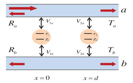
Figure 1: (Color online) Schematic diagram for the quantum routing of single SPs in two channels made of two nanowires coupled to two QDs. Two QDs characterized by $|g_{n}\rangle$ and $|e_{n}\rangle(n=1,2)$ are located at $x=0$ and $x=d$, respectively. An incoming wave from the left side of the nanowire-a will be reflected, transmitted, or transferred into the nanowire-b.

Assume that the QDs are initially in its ground states and a single SP is incident from the left with the energy $E_{k}$. The scattering eigenstate of the Hamiltonian (2) is then given by

$$|\psi\rangle = \sum_{m=a,b}\int dx[\phi_{Rm}(x)C_{Rm}^{\dagger}(x)+\phi_{Lm}(x)C_{Lm}^{\dagger}(x)]$$

$$+ |\emptyset_{a},\emptyset_{b},g_{1},g_{2}\rangle+\xi_{1}|\emptyset_{a},\emptyset_{b},e_{1},g_{2}\rangle+\xi_{2}|\emptyset_{a},\emptyset_{b},g_{1},e_{2}\rangle$$

where $\phi_{Rm(Lm)}$ is the single SP wave function in the right(left) mode of the nanowire-m. $|\emptyset_{a},\emptyset_{b},g_{1},g_{2}\rangle$ denotes that both QD-1 and QD-2 are in their ground states with no SPs. $\xi_{n}(n=1,2)$ is the probability amplitude that the nth QD absorbs the surface plasmon and jumps to its excited state.

The corresponding wave function can also be expressed as

$$\phi_{Ra}(x)=e^{ikx}[\theta(-x)+t_{12}^{a}\theta(x)\theta(d-x)+t_{a}\theta(x-d)],$$

$$\phi_{La}(x)=e^{-ikx}[r_{a}\theta(-x)+r_{12}^{a}\theta(x)\theta(d-x)],$$

$$\phi_{Rb}(x)=e^{ikx}[t_{12}^{b}\theta(x)\theta(d-x)+t_{b}\theta(x-d)],$$

$$\phi_{Lb}(x)=e^{-ikx}[r_{b}\theta(-x)+r_{12}^{b}\theta(x)\theta(d-x)].$$ (4)

where $\theta(x)$ is the Heaviside step function with $\theta(0)=1/2$. $t_{a(b)}$ and $r_{a(b)}$ are the transmission and reflection amplitude in the metal nanowire-a(b), respectively. $t_{12}^{a(b)}\theta(x)\theta(d-x)$ and $r_{12}^{a(b)}\theta(x)\theta(d-x)$ represent the wave function of the SP between QD-1 and QD-2.

Solving the eigenvalue equation $H|\psi\rangle=E_{k}|\psi\rangle$, one get the exact forms of the reflection and transmission coefficients as follows:

$$t_{a}=\frac{B(k)(V_{1b}^{2}E_{k2}+V_{2b}^{2}E_{k1})+B(k)^{2}E_{k1}E_{k2}+V_{1b}V_{2b}[1-e^{i\phi(k)}]M}{B(k)(Q_{1}E_{k2}+Q_{2}E_{k1})+B(k)^{2}E_{k1}E_{k2}+[1-e^{i\phi(k)}]M^{2}+N^{2}},$$

$$r_{a}=\frac{-B(k)[V_{1a}^{2}E_{k2}+V_{2a}^{2}e^{i\phi(k)}E_{k1}]-[1-e^{i\phi(k)}]V_{1a}^{2}V_{2a}^{2}+V_{2a}V_{1b}e^{i\phi(k)}(V_{1a}V_{2b}+N)-V_{1a}^{2}V_{2b}^{2}}{B(k)(Q_{1}E_{k2}+Q_{2}E_{k1})+B(k)^{2}E_{k1}E_{k2}+[1-e^{i\phi(k)}]M^{2}+N^{2}},$$

$$t_{b}=\frac{-B(k)(V_{1a}V_{1b}E_{k2}+V_{2a}V_{2b}E_{k1})-[1-e^{i\phi(k)}]V_{2a}V_{1b}M}{B(k)(Q_{1}E_{k2}+Q_{2}E_{k1})+B(k)^{2}E_{k1}E_{k2}+[1-e^{i\phi(k)}]M^{2}+N^{2}},$$

$$r_{b}=\frac{-B(k)[V_{1a}V_{1b}E_{k2}+V_{2a}V_{2b}e^{i\phi(k)}E_{k1}]-[1-e^{i\phi(k)}]V_{1a}V_{1b}Q_{2}}{B(k)(Q_{1}E_{k2}+Q_{2}E_{k1})+B(k)^{2}E_{k1}E_{k2}+[1-e^{i\phi(k)}]M^{2}+N^{2}}$$ (5)

where $Q_{1}=V_{1a}^{2}+V_{1b}^{2}$, $Q_{2}=V_{2a}^{2}+V_{2b}^{2}$, $M=V_{1a}V_{2a}+V_{1b}V_{2b}$, $N=V_{1a}V_{2b}-V_{1b}V_{2a}$, $E_{kn}=A(k-k_{0})^{2}+\delta_{n}-i\gamma_{n}$, $\delta_{n}=\omega_{c}-\omega_{n}$, $\phi(k)=2kd$, and $B(k)=iA(2k_{0}-k)$. The transmission amplitude $T_{a(b)}=|t_{a(b)}|^{2}$ and reflection amplitude $R_{a(b)}=|r_{a(b)}|^{2}$ can then be determined algebraically.

II Quantum routing of the SPs

The routing property of single SPs is characterized by the transmission and reflection coefficients of these forts. It can be checked numerically for the relation $T_{a}+R_{a}+T_{b}+R_{b}=1$ in the nondissipative case $(\gamma_{1}=\gamma_{2}=0)$, which means that the transmission and reflection probabilities are conserved.

As a contrast, we first discuss the scattering properties of SPs in the single-dot case, in which the inter-dot distance $d$ in Fig. 1 is taken to be in the limit of $d\rightarrow 0$. As shown in Fig. 2, the transmission in four ports of the incident SP is affected slightly when the detuning ($\delta=\delta_{1}=\delta_{2}$) is positive, while two peaks (dips) can emerge for negative detuning. To explain this clearly, we reduce the Eq. (5) and get the reduced forms of $t_{a}=[2V^{2}+B(k)E_{k1}]/[4V^{2}+B(k)E_{k1}]$ and $r_{a}=t_{b}=r_{b}=2V^{2}/[4V^{2}+B(k)E_{k1}]$, with the same coupling $V$. Obviously, for negative detuning in $E_{k1}$ under the quadratic dispersion relation, it yields two different values corresponding to the two dips (peaks) in the curves.

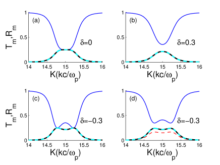
Figure 2: (Color online) Transmission $T_{m}$ (thin solid blue $T_{a}$ and thick solid black $T_{b}$ ) and reflection $R_{m}$ (thin dashed red $R_{a}$ and thick dashed cyan $R_{b}$) spectra of the single-QD case for different detunings $\delta$ (a) $\delta=0$, (b) $\delta=0.3$, (c) $\delta=-0.3$, and (d) $\delta=-0.3$, with $V_{a}=V_{b}=1$ in (a), (b), and (c), and $V_{b}=1.2V_{a}$ in (d). Here, the detuning is defined as: $\delta=\delta_{1}=\delta_{2}$. In (a), (b), and (c), the curves of $R_{a}$, $T_{b}$, and $R_{b}$ overlap each other, while $R_{a}$ separates in (d) for different couplings. Throughout the paper, $\delta$ is in unit of $10^{-6}\omega_{p}$, $V_{a}$ and $V_{b}$ are in the same unit of $1.5\sqrt{10^{-10}\omega_{p}c/4\pi}$, and $k_{0}$ is in unit of $\omega_{p}/c$.

To describe the transfer rate of Sps from the input channel into another channel, the parameters $P_{a}=T_{a}+R_{a}$ and $P_{b}=T_{b}+R_{b}$ are introduced to present the probabilities of finding the incident single SPs in nanowire-a and nanowire-b, respectively. Fig. 3 exhibits the $P_{a}$ and $P_{b}$ for different inter-dot distance $d$ with $V_{a}=V_{b}=1$ and $\delta_{1}=\delta_{2}=0$, respectively. $P_{b}\leq 0.5$ indicates that a single SP incident from the input channel can be redirected into another channel with a maximum probability of 0.5, which is similar to the single-emitter case investigated in Refs. Zhou ; Lu . Interestingly, when the two QDs are separated, the transfer rate $P_{b}$ can be more than 0.5 in a wide rang of wavenumbers near $k_{0}$. Indeed, as seen in Fig. 3 (d), a wide region of $P_{b}>0.5$ is exhibited when $d>0$, and the transfer rate $P_{b}$ is a periodic function of the distance $d$ related to the phase shift $\phi$. This indicates that the present double-dot configuration may provide an effective approach to enhance the routing capability of the SPs.

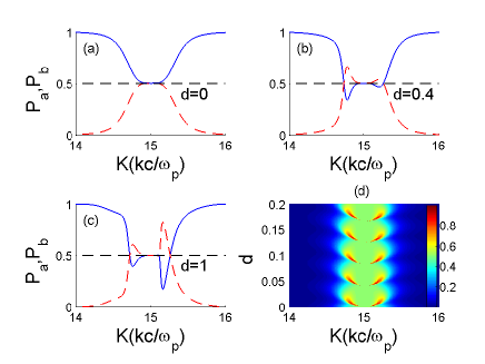
Figure 3: (Color online) $P_{a}$ (solid blue) and $P_{b}$ (dashed red) for different inter-dot distance (a) $d=0$, (b) $d=0.4$, (c) $d=1$, respectively. (d) $P_{b}$ as functions of the distance $d$ and the reduced wavenumber $K$. Other parameters are $\delta_{1}=\delta_{2}=0$, and $V_{a}=V_{b}=1$. Throughout the paper, $d$ is in unit of $5c/\omega_{p}$.

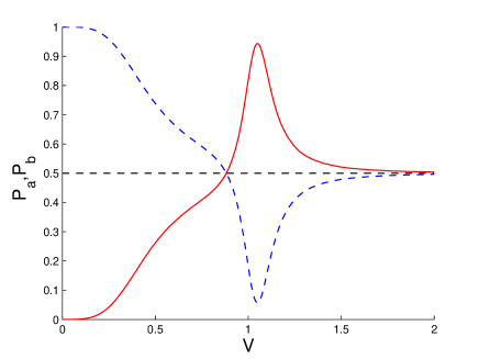
Figure 4: (Color online) The influence of QD-SP coupling on the $P_{a}$ (dashed blue) and $P_{b}$ (solid red). These parameters are $\delta_{1}=\delta_{2}=0$, $d=1$, and $k=1.01k_{0}$.

Furthermore, to investigate the dependence of the transfer rate of the single SPs on the QD-SP coupling, in Fig. 4 we plot $P_{b}$ and $P_{a}$ versus the coupling $V=V_{a}=V_{b}$ at a fixed wavevector $k=1.01k_{0}$. As seen, when the coupling is tuned off, the input SPs is almost completely transmitted, with the transmission $T=1$ in the right-going direction. While the coupling is switched on, the transfer rate from nanowire-a to nanowire-b can reach the maximum value (i.e., $P_{b}\approx 0.95$), and thus high transfer rate is realized. The transfer rate $P_{b}$ is also plotted for the different couplings in Fig. 5, which describes the quantum routing in detail. One can see that, when the couplings $V_{a}$ and $V_{b}$ are sufficiently small, the input SPs cannot be redirected into another channel completely. When increasing the couplings, a large region of high transfer appears, and a perfect transfer rate ($P_{b}\approx 1$) is achieved when the $V_{a}=V_{b}$ is designed as around $1.05$. Therefore, it is possible to efficiently control the routing capability of the single SPs from the a channel into another channel via designing the QD-SP coupling accordingly.

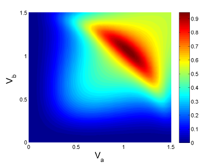
Figure 5: (Color online) The influence of different couplings on the $P_{b}$. These parameters are $\delta_{1}=\delta_{2}=0$, $d=1$, and $k=1.01k_{0}$.

To gain a deeper insight into the dependence of the routing capability of SPs on more controllable parameters, Fig. 6 displays the transfer rate $P_{b}$ of the single SPs versus the QD-SP coupling and the phase shift $\phi$ related to the distance $d$. We can find that the transfer rate $P_{b}$ is a periodic function of the phase shift $\phi$, and there is a wide window of $P_{b}>0.5$ when increasing the QD-SP coupling. For high transfer rate from one channel to the other, a long and narrow region emerges.

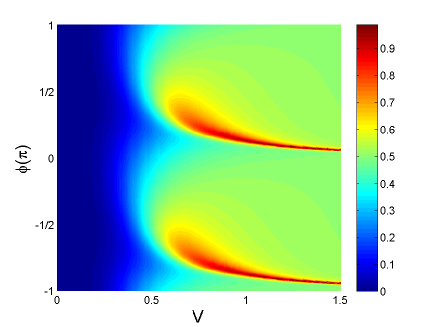
Figure 6: (Color online) The influence of coupling and phase shift on the $P_{b}$. The relevant parameters are set as: $\delta_{1}=\delta_{2}=0$, $V_{a}=V_{b}=V$, and $k=1.01k_{0}$.

III Fano-like resonances of the SPS

With the further increase of $d$, the jiggling behavior in the scattering spectra emerges and becomes more obvious, as shown in Fig. 7(c) and (d). The oscillations may originate from the multiple interference of waves in the region between the two QDs Zhou2 . As the inter-resonator distance increases, more wave interference results in much larger oscillations of the scattering spectra.

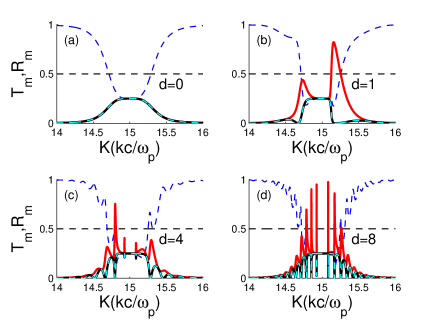
Figure 7: (Color online) Fano-like resonances of transmission ( thin dashed blue $T_{a}$ and thick solid red $T_{b}$ ) and reflection ( thick solid black $R_{a}$ and thin dashed cyan $R_{b}$) spectra for different inter-dot distance in (a) $d=0$, (b) $d=1$, (c) $d=4$, and (d) $d=8$, respectively. Other parameters are $\delta_{1}=\delta_{2}=0$, and $V_{a}=V_{b}=1$.

More interestingly, the feature of Fano resonance in the jiggling spectra becomes also more evident when increasing $d$. Obviously, Fano-line shapes don’t emerge for the single-dot case ($d=0$), whereas Fano resonance occurs at $d=4$. In particular, more sharp peaks (dips) of Fano-line shapes are generated by the nonlinear dispersion relation at $d=8$ for the the transmission (reflection) spectra.

Specifically, to mathematically illustrate the feature related to Fano resonance, we consider one of the reflection coefficients as an example. When $V_{a}=V_{b}=V$ and $\delta_{1}=\delta_{2}=\delta$, the reduced form of the reflection coefficient $R_{b}$ for the quadratic dispersion relation (1) is expressed as

$$R_{b}={\bigg{|}}\frac{B(k)V^{2}E_{k1}[1+e^{i\phi(k)}]+2V^{4}[1-e^{i\phi(k)}]}{4B(k)V^{2}E_{k1}+B(k)^{2}E_{k1}^{2}+2V^{2}[1-e^{i\phi(k)}]}{\bigg{|}}^{2}.$$ (6)

Obviously, the zero value of $R_{b}$ emerges when two functions

$$X=A(2k_{0}-k)[A(k-k_{0})^{2}+\delta]\cos{(kd)}$$ (7)

and

$$Y=2V^{2}\sin{(kd)}$$ (8)

coincide with each other. Fig. 8(a) displays multiple Fano-line shapes for the reflection spectra of $R_{b}$ under the parameter conditions: $d=8$, $V=1$, and $\delta=0$. Fig. 8(b) demonstrates that many intersections of functions $X$ (thin blue curve) and $Y$ (thick red solid curve) represent correspondingly the zeros of $R_{b}$, where multiple Fano-line shapes appear in the jiggling spectra. From Eqs. (6) and (7), one knows that a number of intersections of functions occur under the nonlinear condition, which reveals the appearance of multiple Fano-like resonance in the case is due to the quadratic dispersion relation.

Fano-like resonances in such similar manners have been investigated in recent works Chen5 ; Chen6 ; Chen7 . Physically, in the present double-dot configuration, QD-1 (QD-2) is served as a delocalized (localized) channel for the SPs passing through it. Consequently, the interference between the localized and delocalized channels of the incident SPs results in asymmetric line shapes around these double-peak profiles. Increasing the inter-dot distance would enhance the interference between the two channels and thus lead to more distinct Fano-line shapes.

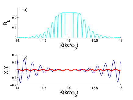
Figure 8: (Color online) (a) Reflection spectra $R_{b}$ with $d=8$, $V_{a}=V_{b}=V=1$, and $\delta_{1}=\delta_{2}=\delta=0$. (b) The intersections of functions $X$ (thin blue curve) and $Y$ (thick red curve) represent the zeros of $R_{b}$. Here $X$ and $Y$ are in the same unit of $\omega_{p}$.

IV Conclusion

In summary, by using the real-space Hamiltonian with nonlinear dispersion relation, we investigate the routing properties of the SPs propagating on the surface of two metal nanowires coupled to two QDs. We find that, for the single-dot case, the transport of the incident SPs exhibit two peaks and dips in the scattering spectra for negative detunings, due to the quadratic dispersion of the waveguides. While for the double-dot case, the jiggling behavior and distinct Fano-like resonance emerge in the scattering spectra. More importantly, our results show that the routing capability of the SPs inputting from one channel to another can be enhanced to exceed 0.5. Sufficiently high transfer rate is also available by properly designing the inter-dot distance and the QD-SP coupling.

Noted that the dissipations are not considered in our investigations. In real experiments, the QD-SP system inevitably experience dissipations, such as the excited-state relaxation of the quantum dots and plasmon loss, since it is also coupled to the environment. However, in contrast with the strong QD-SP coupling, the dissipative scale of the QD exciton ($\hbar$/lifetime $\approx 1\mu eV$) is smaller by two to three orders of magnitude. Therefore, the influence of the dissipations to the routing properties demonstrated above should not be dominant, although it may lower a little the probabilities of the scattering coefficients.

- (1) H. J. Kimble, Nature (London) 453, 1023 (2008).
- (2) J. L. O’Brien, A. Furusawa, and J. Vuckovic, Nat. Photonics 3, 687 (2009).
- (3) L. Zhou, L. P. Yang, Y. Li, and C. P. Sun, Phys. Rev. Lett. 111, 103604 (2013).
- (4) J. Lu, L. Zhou, L. M. Kuang, and F. Nori, Phys. Rev. A 89, 013805 (2014).
- (5) W. B. Yan, B. Liu, L. Zhou, and H. Fan, Europhys. Lett. 111, 64005 (2015).
- (6) G. S. Agarwal and S. Huang, Phys. Rev. A 85, 021801 (2012).
- (7) K. Xia and J. Twamley, Phys. Rev. X 3, 031013 (2013).
- (8) K. Lemr, K. Bartkiewicz, A. Černoch, and J. Soubusta, Phys. Rev. A 87, 062333 (2013).
- (9) X. M. Li, L. Y. Xie, and L. F. Wei, Phys. Rev. A 92, 063840 (2015).
- (10) X. M. Li and L. F. Wei, Phys. Rev. A 92, 063836 (2015).
- (11) J. Lu, Z. H. Wang, and L. Zhou, Opt. Express 23, 22955(2015).
- (12) T. Aoki, A. S. Parkins, D. J. Alton, C. A. Regal, B. Dayan, E. Ostby, K. J. Vahala, and H. J. Kimble, Phys. Rev. Lett. 102, 083601 (2009).
- (13) I. C. Hoi, C. M. Wilson, G. Johansson, T. Palomaki, B. Peropadre,
- (14) I. Shomroni, S. Rosenblum, Y. Lovsky, O. Brechler, G. Guendelman, and B. Dayan, Science 345, 903(2014).
- (15) M. S. Tame, K. R. McEnery, S. K. Özdemir, J. Lee, S. A. Maier and M. S. Kim, Nature Physics 9, 329(2013).
- (16) R. Zia and M. L. Brongersma, Nat. Nanotechnology 2, 426 (2007).
- (17) K. Yu. Bliokh, Yu. P. Bliokh, V. Freilikher, S. Savel’ev, and F. Nori, Rev. Mod. Phys. 80, 1201 (2008).
- (18) S. Savel’ev, V. A. Yampol’skii, A. L. Rakhmanov, and F. Nori, Rep. Prog. Phys. 73, 026501 (2010).
- (19) A. V. Akimov, A. Mukherjee, C. L. Yu, D. E. Chang, A. S. Zibrov, P. R. Hemmer, H. Park, and M. D. Lukin, Nature (London) 450, 402(2007).
- (20) Y. Fedutik, V. V. Temnov, O. Schops, U.Woggon, and M. V. Artemyev, Phys. Rev. Lett. 99, 136802 (2007).
- (21) D. E. Chang, A. S. Søensen, E. A. Demler, and M. D. Lukin, Nat. Phys. 3, 807 (2007).
- (22) F.-Y. Hong, S.-J. Xiong, Nanoscale Res. Lett. 3, 361 (2008).
- (23) N.-C. Kim, J.-B. Li, Z.-J. Yang, Z.-H. Hao, and Q.-Q. Wang, Appl. Phys. Lett. 97, 061110 (2010).
- (24) J.-H. Li, and R. Yu, Opt. Lett. 19, 20991 (2011).
- (25) W. Chen, G. Y. Chen, and Y. N. Chen, Opt. Lett. 36, 3602 (2011).
- (26) G. Y. Chen and Y. N. Chen, Opt. Lett. 37, 4023 (2012).
- (27) M.-T. Cheng and Y.-Y. Song, Opt. Lett. 37, 978 (2012).
- (28) G. Y. Chen, N. Lambert, C. H. Chou, Y. N. Chen, and F. Nori, Phys. Rev. B 84, 045310 (2011).
- (29) G. Y. Chen, C. M. Li, Y. N. Chen, Opt. Lett. 37, 1337 (2012).
- (30) M.-T. Cheng, Y.-Q. Luo, P.-Z. Wang, and G.-X. Zhao, Appl. Phys. Lett. 97, 191903 (2010).
- (31) W. Chen, G. Y. Chen, and Y. N. Chen, Opt. Lett. 18, 10360 (2010).
- (32) G. Y. Chen, Y. N. Chen, and D. S. Chuu, Opt. Lett. 33, 2212 (2008).
- (33) Y. N. Chen, G. Y. Chen, D. S. Chuu, and T. Brandes, Phys. Rev. A 79, 033815 (2009).
- (34) D. E. Chang, A. S. Søensen, P. R. Hemmer, and M. D. Lukin, Phys. Rev. Lett. 97, 053002 (2006).
- (35) J. T. Shen, S. Fan, Phys. Rev. A 79, 023837 (2009).
- (36) L. Zhou, H. Dong, Y. X. Liu, C. P. Sun, and F. Nori, Phys. Rev. A 78, 063827 (2008)
- (37) G. Y. Chen, Y. N. Chen, Opt. Lett. 37, 4023 (2012).
- (38) G. Y. Chen, M. H. Liu, Y. N. Chen, Phys. Rev. A 89, 053802 (2014).