Trapping of Rydberg Atoms in Tight Magnetic Microtraps

Abstract

We explore the possibility to trap Rydberg atoms in tightly confining magnetic microtraps. The trapping frequencies for Rydberg atoms are expected to be influenced strongly by magnetic field gradients. We show that there are regimes where Rydberg atoms can be trapped. Moreover, we show that so-called magic trapping conditions can be found for certain states of rubidium, where both Rydberg atoms and ground state atoms have the same trapping frequencies. Magic trapping is highly beneficial for implementing quantum gate operations that require long operation times.

I Introduction

Atoms with one electron excited to a high principle quantum number $n$, commonly known as Rydberg atoms Gallagher (2005), have been proposed as the basis for quantum simulators and quantum information processing Saffman et al. (2010); Müller et al. (2011). An idea going back to Richard Feynman Feynman (1982), a quantum simulator is an easily manipulated quantum system onto which the Hamiltonian of other quantum problems can be mapped. Ever since, quantum simulation and information processing has been driven by the promise of access to complex quantum systems as well as applications in quantum technology fla (2017).

In this context, Rydberg atoms attract a lot of attention due to their extreme properties like $n^{11}$ scaling of the $C_{6}$ Van der Waals coefficient and the blockade effect, providing strong interactions and the essential mechanism for quantum gates Saffman et al. (2010); Lukin et al. (2001); Jaksch et al. (2000). An important issue is to achieve so-called magic trapping, identical trapping potentials for the ground state and the Rydberg state. Magic trapping conditions can suppress decoherence due to atomic motion during quantum gate protocols, much needed for high-fidelity quantum operations Wilk et al. (2010); Saffman (2016). However, this is challenging to realize for alkali atoms in optical traps Zhang et al. (2011); Topcu and Derevianko (2014).

In this paper we show that magic trapping conditions can be a chieved more easily in magnetic lattice traps Wang et al. (2016). Both ground state and Rydberg atoms can be trapped in magnetic fields arising from microwires on a fabricated chip Reichel et al. (1999); Folman et al. (2000, 2002); Reichel (2002), or from a patterned magnetic film giving rise to an array of microtraps Leung et al. (2014); Whitlock et al. (2009); Wang et al. (2017). These microtraps have very strong magnetic field gradients, hence are very tight, and can be arranged into different lattice geometries, such as square or hexagonal. Field gradients can be particularly strong using patterned magnets. Whereas gradients above microwires are typically 10-100 T/m, with magnetic film chips they can be readily two orders of magnitude higher. If the blockade radius is comparable to, or larger than, a single trap, each trap effectively becomes a single excitation site. In this paper we investigate the magnetic trappability of alkali Rydberg atoms, and address the issue of achieving magic trapping conditions.

For ground state atoms the magnetic field can be assumed to be uniform across the atom. However, the large classical electron orbit radii of the Rydberg atoms and the large gradients of the microtraps make this approximation invalid. Magnetic trapping of Rydberg atoms in other magnetic configurations has been studied by other authors Choi et al. (2005); Singh et al. (2008); Lesanovsky and Schmelcher (2005a, b); Schmidt et al. (2007); Hezel et al. (2006, 2007); Mayle et al. (2009a, b). Our paper is related to the work performed by Mayle, Lesanovsky and Schmelcher (MLS) Mayle et al. (2009a, b), however, our work is focused on the strong gradient regime of the microtraps, requiring a higher order expansion of the magnetic fields.

In this work we base our calculations on ⁸⁷Rb atoms, however, the treatment is generally applicable to other species as well. For a 50 kHz trap the oscillator length of a rubidium atom (34 nm) is much smaller than the rms radius of a $n=50$ electron orbit (132 nm). The strong magnetic field gradient then results in a magnetic field difference of 0.9 G across the size of the atom, resulting in an energy difference of about 1.3 MHz, much larger than the trapping frequency. This paper therefore considers the effect of the spatial extent of the electronic wave function on the trappability of the Rydberg atom in a magnetic trap.

In accordance with the Born-Oppenheimer approximation, we assume that the motion of the Rydberg electron and the atomic core can be separated, and that the light Rydberg electron will react instantly to any movement of the heavy core. We then use perturbation theory in the fine structure basis to find the energy of the Rydberg electron as function of the position of the core in the trap. These energies can be regarded as potentials for the core, which we call Potential Energy Surfaces (PES). We have expanded these potentials as harmonic traps around their respective minima and found feasible trapping conditions for a wide range of Rydberg states.

This paper is divided into six sections. In section II we provide a detailed description of the magnetic field configuration used in this work. In section III we provide the model Hamiltonian in Jacobi coordinates and discuss some of the differences to the earlier work by MLS. Furthermore, we discuss the perturbative treatment of the system. In sections IV and V we discuss the outcome of the previous sections, with focus on trapping Rydberg atoms and magic trapping conditions. In section VI we conclude on our work.

II Parametrization of the magnetic traps

In the following two sections we use atomic ($\hbar=m_{e}=a_{0}=1$) units and summation over repeated indices for the sake of readability. We model the magnetic field as a Ioffe-Pritchard configuration around the trap minimum Gerritsma and Spreeuw (2006)

$$\bm{B}(\bm{x})=\begin{pmatrix}0\\ 0\\ \mathcal{B}\end{pmatrix}+\mathcal{G}\begin{pmatrix}x_{1}\\ -x_{2}\\ 0\end{pmatrix}+\frac{1}{2}\hat{\bm{e}}_{i}c_{ijk}x_{j}x_{k}.$$ (1)

We shall call these terms constant $\bm{B}_{c}$, linear $\bm{B}_{l}$ and quadratic $\bm{B}_{q}$ respectively. The strength of the constant term is set to 3.23G. At this field the differential Zeeman shift between the two qubit states $\left|F=1,m_{F}=-1\right>$ and $\left|F=2,m_{F}=1\right>$ vanishes Davis (2002).

Expanding the magnetic fields to quadratic order goes beyond existing works in literature Mayle et al. (2009a). This is necessary for the systems with strong magnetic gradients we explore. This provides further accuracy for systems already investigated with linear only expansions, which can never explain axial trapping.

The linear term coefficient $\mathcal{G}$ provides confinement in the tight transverse directions. This coefficient has a value of 900 T/m for microtraps in a hexagonal lattice Leung et al. (2014). In the remainder of this paper we use microtrap parameters as relevant for this hexagonal lattice. This is much greater than that of more conventional Z-wire magnetic chip traps with $\mathcal{G}\approx 7$ T/m Naber (2016).

The curvature tensor $c_{ijk}$, which determines the strength of the quadratic term of the magnetic field, is symmetric under permutation of its indices and all partial traces vanish. This leaves 7 independent components. For the microtraps the non zero components of $c_{ijk}$ are on the order of $10^{7}$ T/m², again much larger than for a typical Z-wire trap, where the non zero components are on the order of 10-100 T/m².

Choosing the Coulomb gauge we find the vector potential corresponding to Eq. (1)

$$\bm{A}(\bm{x})=\frac{\mathcal{B}}{2}\begin{pmatrix}-x_{2}\\ x_{1}\\ 0\end{pmatrix}+\mathcal{G}\begin{pmatrix}0\\ 0\\ x_{1}x_{2}\end{pmatrix}+\frac{1}{8}\hat{\bm{e}}_{i}\epsilon_{ijk}c_{jlm}x_{l}x_{m}x_{k},$$ (2)

with $\epsilon_{ijk}$ the fully antisymmetric Levi-Civita tensor. We retain the naming convention from the magnetic field, i.e. the curl of the ’linear’ term of the vector potential corresponds to the linear term of the magnetic field $\nabla\times\bm{A}_{l}=\bm{B}_{l}$ etc. It is convenient to define ”residual terms” for the magnetic field and the vector potential respectively, as follows

$$\tilde{\bm{B}}(\bm{R},\bm{r})= \bm{B}(\bm{R}+\bm{r})-\bm{B}(\bm{R})-\bm{B}(\bm{r})$$ (3)

$$\tilde{\bm{A}}(\bm{R},\bm{r})= \bm{A}(\bm{R}+\bm{r})-\bm{A}(\bm{R})-\bm{A}(\bm{r}).$$ (4)

Note that these do not describe the fields at any position, but merely express the difference between the sum of fields at two positions and the field at the sum of those two positions.

III Hamiltonian and perturbation terms

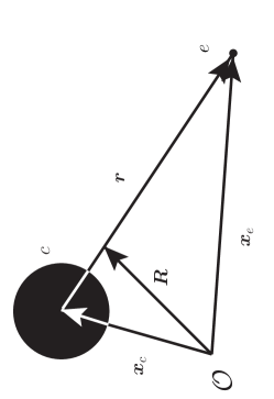
Figure 1: Schematic of the coordinates used in this paper. $\mathcal{O}$ denotes the origin. $\bm{x}_{e}$ and $\bm{x}_{c}$ are the position vectors of the electron and core respectively in the Ioffe-Pritchard frame. $\bm{r}$ and $\bm{R}$ denotes the relative and center of mass coordinates respectively. Since the mass is almost entirely contained in the core we approximate $\bm{R}$ with $\bm{x}_{c}$.

Our approach builds on a spin and minimal coupling scheme for the valence electron with position $\bm{x}_{e}$, momentum $\bm{p}_{e}$ and mass $m_{e}=1$ and the core with position $\bm{x}_{c}$, momentum $\bm{p}_{c}$ and mass $M$ in an external magnetic field. We reexpress this Hamiltonian using Jacobi coordinates ($(x,y,z)^{T}=\bm{r}=\bm{x}_{e}-\bm{x}_{c}$, $(X,Y,Z)^{T}=\bm{R}=\bm{x}_{e}/M+\bm{x}_{c}$, see Fig. 1). Since the mass ratio is large, about $1.6\times 10^{5}$ for ⁸⁷Rb, we identify the core $\bm{x}_{c}$ and center of mass coordinate $\bm{R}$ as an approximation. This leaves us with the Hamiltonian

$$\mathcal{H}= \mathcal{H}_{\mathrm{ff}}+\bm{A}\left(\bm{R}+\bm{r}\right)\cdot\bm{p}+\bm{S}\cdot\bm{B}\left(\bm{R}+\bm{r}\right)$$

$$+\frac{\bm{P}^{2}}{2M}+\frac{1}{M}\left[\bm{A}\left(\bm{R}+\bm{r}\right)-\bm{A}\left(\bm{R}\right)\right]\cdot\bm{P}$$ (5)

$$+\frac{1}{2}\bm{A}^{2}\left(\bm{R}+\bm{r}\right)+\frac{g_{I}}{2}\bm{I}\cdot\bm{B}\left(\bm{R}\right),$$

with $\mathcal{H}_{\mathrm{ff}}$ being the (field free) fine structure Hamiltonian, $\bm{P}$ the center of mass momentum operator, $\bm{S}$ the electron spin, $\bm{I}$ the nuclear spin and $g_{I}$ the nuclear Landé g-factor. We apply degenerate perturbation theory in the fine structure basis $\left|\kappa\right>=\left|nLjm_{j}\right>$ to this Hamiltonian, coupling to all states within one $L$-manifold.

At this point, in previous work Mayle et al. (2009a, b) a unitary transformation is applied: $U_{\mathrm{lit}}=\exp(-i(\bm{B}_{c}\times\bm{r})\cdot\bm{R}/2)=\exp(i\bm{A}_{c}(\bm{R})\cdot\bm{r})$. This removes, what they consider the most dominant perturbation terms in the linear field approximation, $\bm{A}_{c}^{2}(\bm{R})/2$ and $-\bm{A}_{c}(\bm{R})\cdot\bm{p}$, which are of similar magnitude but opposite sign, making the perturbative treatment more robust. However, this transformation complicates the diamagnetic terms unnecessarily. If we consider Eq. (20) in Ref. Mayle et al. (2009a) along the line $X=Y$ we obtain $E^{(2)}_{\kappa}(\bm{R})\approx C_{z}\mathcal{G}^{2}X^{4}$ with $C_{z}\approx-1/2$, within 10% for $35\leq n\leq 45$ and $l\leq 4$. But if we consider the term $\bm{A}^{2}_{l}(\bm{R})/2=\mathcal{G}^{2}X^{2}Y^{2}/2$, which is implicitly neglected by MLS, we find the same value but with opposite sign along $X=Y$. Thus the main Rydberg contribution is countered by a neglected term.

Instead we use a more general unitary transformation that does not rely on any explicit field to be introduced, and is inspired by the previous

$$U=\exp\left(i\bm{A}(\bm{R})\cdot\bm{r}\right).$$ (6)

We apply this to the Hamiltonian: $H=U\mathcal{H}U^{\dagger}$. The transformation (6) removes the terms $\bm{A}^{2}(\bm{R})/2$ and $-\bm{A}(\bm{R})\cdot\bm{p}$, in their entirety in contrast to the standard transformation $U_{\mathrm{lit}}$.

The resulting Hamiltonian can be split into four parts ($H=H_{R,r}+H_{R}+H_{r}+H_{r,P}$) according to their dependence on the Jacobi operators

$$H_{R,r}= H_{\mathrm{ff}}+\left(\bm{S}+\frac{1}{2}\bm{L}_{r}\right)\cdot\bm{B}(\bm{R})+\frac{1}{2}\tilde{\bm{A}}^{2}(\bm{R},\bm{r})$$

$$+ \bm{A}(\bm{r})\cdot\tilde{\bm{A}}(\bm{R},\bm{r})+H_{\mathrm{small}},$$ (7)

$$H_{R}= \frac{\bm{P}^{2}}{2M}+\frac{1}{2}g_{I}\bm{I}\cdot\bm{B}(\bm{R}),$$ (8)

$$H_{r}= \left(\bm{B}_{l}(\bm{r})+\bm{B}_{q}(\bm{r})\right)\cdot\bm{S}+\left(\bm{A}_{l}(\bm{r})+\bm{A}_{q}(\bm{r})\right)\cdot\bm{p}$$

$$+ \frac{1}{2}\bm{A}^{2}(\bm{r}),$$ (9)

$$H_{r,P}= \frac{1}{M}\left[\bm{A}(\bm{R}+\bm{r})-\bm{A}(\bm{R})+\nabla_{R}\left(\bm{A}(\bm{R})\cdot\bm{r}\right)\right]\cdot\bm{P},$$ (10)

with $H_{\mathrm{small}}$ collecting some terms we can neglect in perturbation theory, and $\bm{L}_{r}$ being the electron angular momentum operator. For the ground state, only the $\bm{B}(\bm{R})$ term of Eq. (7) contributes significantly to the energy, as $\langle|\bm{r}|\rangle\approx 0$, and the magnetic trapping field is assumed to be constant across the atom. This is sharply contrasted for large Rydberg states, where terms dependent on $\bm{r}$ become important, since $\langle|\bm{r}|\rangle\propto n^{2}$ is large, and the terms

$$\frac{1}{2}\tilde{\bm{A}}^{2}(\bm{R},\bm{r})+\bm{A}(\bm{r})\cdot\tilde{\bm{A}}(\bm{R},\bm{r})+H_{r},$$ (11)

which we call the ”Rydberg term”, become important. These terms are mostly extra terms compared to the MLS approach, and together constitute the Rydberg specific part of the Hamiltonian.

We work in a frozen gas setting where $P/M\approx 0$. This has the direct consequence that we can neglect the $H_{r,P}$. Further more, this setting is well explored with the Born-Oppenheimer approximation, where the electrons are assumed to react instantly to any core movement. In accordance with the Born-Oppenheimer approximation we assume the eigenstates to be product states of a $\bm{r}$ dependent part and a $\bm{R}$ dependent part

$$|\psi\rangle=\left|\psi_{\bm{r}}\right>\left|\psi_{\bm{R}}\right>=\sum_{\kappa}c_{\kappa}\left|\kappa\right>\left|\psi_{\bm{R}}\right>,$$ (12)

where $c_{\kappa}$ are expansion coefficients for $\psi_{\bm{r}}$ in the fine structure basis.

By applying the electronic parts (i.e. the parts dependent on the relative coordinate) of the Hamiltonian, we find an energy dependent on the core position $\bm{R}$

$$(H_{R,r}+H_{r})\left|\psi\right>=E(\bm{R})\left|\psi\right>.$$ (13)

We specifically use degenerate perturbation theory to find the electronic energies $E(\bm{R})$ at any given core position $\bm{R}$. We use a set of all fine structure states $|\kappa\rangle=|nLjm_{j}\rangle$ (the eigenstates of $H_{\mathrm{ff}}$), within one $n$, $L$- manifold, as basis for our perturbative treatment, as the energy contribution from the fine structure Hamiltonian is, by far, most dominant. We have found that coupling between states with different $n$ or $L$ quantum numbers is not significant for the parameter space we are considering, and we have not included this in our model.

The complexity of this computation can be greatly reduced by carefully examining and understanding the couplings between different states. The expressions become quite simple and $S_{1/2}$ states can be solved analytically. We include mixing between different $j$ states within one $L$ manifold, as they are sufficiently close in energy for the principal quantum numbers of interest.

Since the energy in Eq. (13) is dependent on the core position $\bm{R}$ we interpret it as a potential and construct a total potential $W$ seen by the core

$$\langle\psi_{\bm{r}}|H|\psi\rangle= \left[H_{R}+E(\bm{R})\right]|\psi_{\bm{R}}\rangle$$

$$= \left[T_{R}+W(\bm{R})\right]|\psi_{\bm{R}}\rangle.$$ (14)

We call these potentials $W(\bm{R})$ Potential Energy Surfaces (PES). Since the mictrotraps are designed to trap ground state atoms with only little spatial extent, it can be expected that trapping is mostly provided by the unperturbed Hamiltonian. However, there are exceptions leading to anti-trapping, as we will explain below.

IV Potential energy surfaces

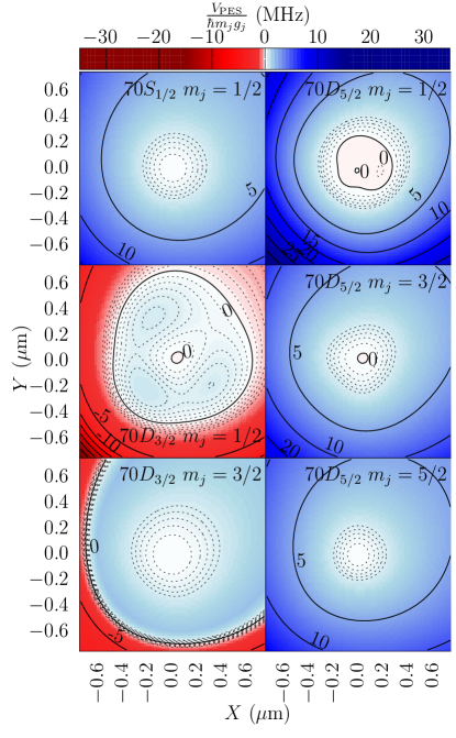
Figure 2: Potential Energy Surfaces (PES) for the different angular states with $n=70$ in the Ioffe-Pritchard plane ($Z=0$) scaled by $m_{j}g_{j}$. These represent results for a typical magnetic potential of the hexagonal magnetic lattice. Solid contours at every 5 MHz and dashed contours at every 0.2 MHz in the interval -1 to 1 (limits included) are shown. Near the origin we observe positive curvature, meaning that the state is trappable, for all but the $70D_{5/2}$ with $m_{j}=1/2$ state; where a small bump indicates a crossover to a Mexican Hat type potential. At higher $n$ this will be more pronounced. For both $70D_{3/2}$ states we observe strong downwards gradients for large $|R|$, due to the strong influence of the diamagnetic term. The noticeable asymmetry in the plots is due to the fact that the coordinates are rotated with respect to the atom chip surface. The $X=Y$ direction is normal to the surface.

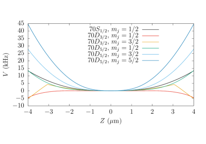
Figure 3: Trapping potential in the $Z$ direction at $X=Y=0$ for the different angular states with $n=70$. Parameters of the hexagonal lattice microtraps have been used Leung et al. (2014). Trapping along this direction is much weaker than in the $X$, $Y$ plane. All states shown have local, albeit weak, minima near $Z=0$.

We have calculated PES states that are reachable via a standard two-photon excitation process ($S$- and $D$ states) from the rubidium ground state. We consider only states where $n\leq 80$ in order to keep perturbations small compared to the fine structure energies and to not break the Born-Oppenheimer approximation. For $nD_{j}$ states mixing becomes significant when $n>80$ and the finestructure states are no longer good quantum states. Thus the results for $nD_{j}$ with $n>80$ are unreliable. In the remainder of this paper we no longer use atomic units, but rather SI units.

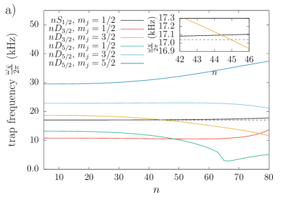
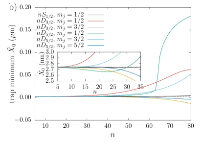
Figure 4: (a) Radial trap frequency and (b) position of the local potential minimum as a function of $n$, both in the $\tilde{X}$ direction. The shift of the trap minimum away from the origin occurs gradually for low $n$ but becomes very rapid for larger $n$. The rapid shift indicates crossover to a Mexican hat type potential. Dashed lines indicates the value of the $5S_{1/2}$, $m_{j}=1/2$ state in all cases. Similar results are found in the $\tilde{Y}$ direction; whereas in the $Z$ direction the trap is an order of magnitude weaker. Of special interest is the $45D_{3/2}$, $m_{j}=3/2$ state, where the trapping frequency is very close to that of the ground state. This and the small value of $X_{0}$ lead to magic trapping conditions for the $45D_{3/2}$, $m_{j}=3/2$ state.

In Fig. 2 we present the PES for the $70L_{j}$ states with all different positive $m_{j}$ up to a distance of 0.75 $\mu$m from the trap center in the radial plane ($Z=0$). These have been rescaled by $m_{j}g_{j}$ to make them comparable. The approximate symmetry with respect to the $X=Y$ line is due to this line being normal to the chip surface. In Fig. 3 we see the $Z$ dependence of the PES for the same states to a distance of 4 $\mu$m from the trap center along the $X=Y=0$ line. The choice of the $70L_{j}$ states is motivated by being well within the limits of our methods while the high $n$ makes the Rydberg specific contributions clearly visible. This is seen in the strong dependence on the angular state, which is not evident for $n<40$. When going to even higher $n$ these effects become more pronounced and we eventually loose trapping for the $nD_{3/2}$ potentials, whereas the $nD_{5/2}$ states transition to quartic trapping potentials.

The $nS_{1/2}$ state trapping potentials do remain fairly similar to that of the ground state, not surprising as the electron is more tightly confined near the core.

The $70D_{3/2}$ states stand out among the PES by being antitrapping on the micrometer scale in both the $Z=0$ plane and along the $X=Y=0$ line. The PES of these states are more strongly influenced by the diamagnetic terms in the Hamiltonian, leading to both the antitrapping behavior and the structure in the positive potential region of the $m_{j}=1/2$ state, by coupling to $(j$, $m_{j})$-states of different angular symmetry. This structure makes the state unsuitable for quantum simulation but shows the importance of the Rydberg nature of the atom to the PES.

We see a small bump near the origin in the PES of the $70D_{5/2}$, $m_{j}=1/2$ state. For higher $n$ this bump becomes a regular peak turning the potential a Mexican hat shape.

In our analysis of the PES of the $n=35$, $45$, $55$, $65$, and $75$ states, we fitted a polynomial to the contributions of the Rydberg specific terms in Eq. (11). This showed that, though highly state dependent, the effect of the Rydberg terms can be reduced to an offset and an $R^{2}$ dependent term for the $nS_{1/2}$ and $nD_{5/2}$ states. When $n>73$, however, this simple picture fails for the $nD_{3/2}$ states, and higher order terms are needed to describe the behavior.

We predict that one can encounter this effect in spectroscopic measurements, even for weaker traps, as long as the magnetic field is well described by the second order expansion of our model.

Our results show that in general, the PES of the $nS_{1/2}$ and $nD_{5/2}$ states are always trapping on micrometer length scales for atoms with $n<80$. The $nD_{3/2}$ states also show trapping PES, but for $n>50$ the PES become of antitrapping nature on the micrometer scale, and we only observe local trapping on sub micrometer scales, and rich structure appearing near the center of the PES, when $m_{j}=1/2$ and $n>60$.

V Trapping conditions

We now analyze the trapping conditions for different Rydberg states as function of principal quantum number $n$ and angular state. We investigate in particular whether Rydberg states with trapping conditions identical to the ground state conditions can be found. This is particularly relevant for the implementation of various quantum information protocols based on Rydberg interactions. Rydberg atoms and ground state atoms experience different trapping potentials, which leads to motional decoherence. We denote a Rydberg atom in internal state $\left|r\right>=\left|nLjm_{j}\right>$ in a certain motional state $\left|\nu\right>$ by $\left|r,\nu\right>$. During the Rydberg excitation that same motional state $\left|\nu\right>$ will be a non-stationary state in the Rydberg trap. When de-exciting the atom the motional state will have changed under time evolution and no longer be identical to $\left|\nu\right>$. Therefore it is of great interest if we can suppress this decoherence mechanism by realizing conditions of magic trapping, where ground and Rydberg state atoms would experience identical trapping potentials.

First, we define the rotated coordinates away from the surface of the chip $\tilde{X}=\sqrt{\frac{1}{2}}(X+Y)$ and $\tilde{Y}=\sqrt{\frac{1}{2}}(X-Y)$ parallel to the surface.

$$V(\tilde{X},\tilde{Y},Z)= C+\frac{1}{2}m\omega^{2}_{\tilde{X}}(\tilde{X}-\tilde{X}_{0})^{2}+\frac{1}{2}m\omega^{2}_{\tilde{Y}}(\tilde{Y}-\tilde{Y}_{0})^{2}$$

$$+\frac{1}{2}m\omega_{Z}^{2}(Z-Z_{0})^{2},$$ (15)

where $C$ is some constant offset, $(\tilde{X}_{0},\tilde{Y}_{0},Z_{0})$ is the minimum position of the trap and $\omega_{i}$ is the local trap frequency around the minimum in the $\tilde{R}_{i}$ direction. This is a good approximation over a distance of $0.3\mu m$ from the trap center, many times larger than the trap oscillator length. Analysis of the traps show that all states have tens or hundreds of trap levels. With energy much lower than the potential walls, the center of mass will behave as in an infinitely deep potential. The lowest number of trap levels are found for the $nD_{3/2}$, $m_{j}=1/2$ states, consistent with the antitrapping long range behavior.

Our analysis shows that the trap behaves harmonically for $n\leq 50$ and does not deviate significantly from the $n=5$ trapping potential for any given angular state, see Fig. 4. In particular the changes in $nS_{1/2}$ state trapping frequency and minimum position remain insignificant over the whole $n$-range considered.

The $nD_{3/2}$ states show strong dependence on $n$ and $m_{j}$. In the $m_{j}=1/2$ states we find the trap bottom shift away from the origin but the effective trap frequency remains relatively stable until $n=70$. The $m_{j}=3/2$ states, show consistently decreasing trap frequencies but the trap minima remain fairly centered. As seen from Fig. 4 magic trapping conditions, i.e. effective trapping similar to that of the ground state, are present for the $nD_{3/2}$, $m_{j}=3/2$ states around $n=45$. The effective trap frequency of these states are equal to that of the ground state in the $\tilde{X}$ direction. This means that the Rydberg excitation cycle can be performed with minimal motional decoherence. Since the PES for these states are nearly identical to that for the ground state, the CM wave function remains unchanged after the Rydberg excitation, see Fig 5.

The $nD_{5/2}$ states show rich behavior in the parameters of the effective trapping. The trap frequencies of states with $m_{j}=1/2$ drop to around a quarter of the $n=5$ value at $n=66$. The minimum of the traps shift position away from the origin, very rapidly for $63\leq n\leq 65$. Inspection of the PES shows that this is a crossover to a Mexican Hat type potential in the $Z=0$ plane. The $m_{j}=3/2$ state trapping frequencies remain stable, at around twice the value of the ground state trap frequency, across the entire $n$-interval considered, with a slight decrease for very large $n$. The minimum position shifts away from the origin. The $m_{j}=5/2$ states show large, increasing trapping frequency, but no significant change in trap minimum position. The $nD_{5/2}$ states are not suitable for procedures requiring trap frequencies comparable to those of the ground state.

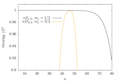
Figure 5: Overlap of the center of mass ground state after 10 $\mu$s spent in an excited state, taking all directions into account. We bring the system into the Rydberg state and de-excite after 10 $\mu$s, we ignore all other decoherence effects like spontaneous emission. This determines the probability of finding the center of mass particle in the ground state after spending some time in a given excited electronic state.

The trapping conditions that were found for the $\tilde{X}$ direction in Fig. 4 for the $45D_{3/2}$, $m_{j}=3/2$ and nearby states (and similar conditions in the $\tilde{Y}$ and $Z$ directions) are expected to strongly suppress motional decoherence in any gate protocol involving Rydberg excitation and de-excitation. A full analysis of gate fidelities should take into account the photon recoils upon (de-)excitation, considering also that these tight magnetic traps are in the Lamb-Dicke limitWineland et al. (1998). For the highest fidelities the anharmonicity of the traps may also play a role. Such full analysis of fidelities is beyond the scope of this paper.

As a first indicator, we have projected the motional ground state of the $5S_{1/2}$, $m_{j}=1/2$ electronic state, denoted by $\left|g,0\right>$, onto the motional states of an electronically excited state,

$$\left|\psi\right>= \sum_{\nu}\left|r,\nu\right>\left<g,0\middle|r,\nu\right>=\sum_{\nu}c_{\nu}\left|r,\nu\right>,$$ (16)

with $\nu=\{\nu_{\tilde{X}},\nu_{\tilde{Y}},\nu_{Z}\}$ being the motional quantum numbers in the indexed directions. We time evolve this projection $\left|\psi(t)\right>=\exp(iHt/\hbar)\left|\psi\right>$ and calculate the time delayed overlap

$$\beta_{t}= \left<\psi(0)\middle|\psi(t)\right>$$

$$= \sum_{\nu}|c_{\nu}|^{2}\exp\left[-i\left(\nu+\frac{3}{2}\right)\omega t\right],$$ (17)

where the coefficients $c_{\nu}$ are calculated using second order perturbation theory,and define the overlap of the state as $|\beta|^{2}=|\beta_{10\mu s}|^{2}$. Thus $1-|\beta|^{2}$ represents the probability of finding the atom in a different motional state after a 10 $\mu$s evolution time.

In Fig. 5 we see that this overlap reaches 0.9994, for the $46D_{3/2}$, $m_{j}=3/2$ state, comparable to that of the $nS_{1/2}$, $m_{j}=1/2$ states, which have overlaps exceeding 0.999 for $n\leq 58$. We have identified two angular configurations that are comparably good, around $n=46$. Experiments therefore can choose between two angular states and therefore also between symmetric and directional blockade regions. The reason that the optimal overlap is found for $46D_{3/2}$, whereas Fig 4 would suggest $n=45$ is due to a small shift of the trap minimum position.

This overlap allows for minimizing decoherence due to changes in effective trapping, making sure the effect of the excited state trap is not the limiting factor. This should be compared to losses due to other sources, which will be dominant, in particular spontaneous emission and transitions driven by black body radiation, with a life time of about 50 $\mu$s for the $n=45$ states Beterov et al. (2009).

VI Conclusion and outlook

We have studied Rydberg atoms in magnetic microtraps described by a second order expansion of the magnetic field. The magnetic microtraps are much tighter and have much stronger field gradients than more commonly used traps, such as Z-wire traps. This enhances the effects of the trap on the spatially extended Rydberg atoms.

Our work confirms the findings by Mayle et al. Mayle et al. (2009a), that Rydberg atoms can indeed be magnetically trapped, and we have extended their model by including several new terms in the Hamiltonian, most importantly thediamagnetic term mixing the relative and center of mass coordinates. These terms constituted an unknown contribution to the trapping potentials of Rydberg atoms that, while negligible in weaker traps, are important in the context of microtraps. We have, however, also found the ’Rydberg term’ of Ref. Mayle et al. (2009a) to be almost zeroed by some of the additional terms.

We found that trapping of Rydberg atoms is possible for both $S$-states and $D$-states, but for high $n$ effective trapping potentials become distorted, due to the anisotropic nature of the Rydberg contributions and the increased contribution from the diamagnetic terms.

We have found near-magic trapping conditions with more than 99% overlap for $nS$ states with $n<70$ and $nD_{3/2}$ states with $m_{j}=3/2$ and $43\leq n\leq 49$, with the highest overlap for the $n=46$ state. This provides a choice between the two angular states, and therewith the angular dependence of the interaction. With magic trapping states available, a Rydberg equivalent of the Mølmer-Sørensen gate Sørensen and Mølmer (1999, 2000); Wang et al. (2001), relying on such conditions, could be possible. Such a gate implementation will be of great value for quantum simulation and processing, and demands further research.

We have found that the spatially extended nature of Rydberg atoms has significant effects in the microtraps, and results significant modifications of the trapping potentials of the center of mass. In particular we have observed a strong $n$-dependence of the center of mass trapping potentials, with shallow trapping for $nD_{3/2}$ states and quartic trapping of $nD_{5/2}$ states.

Further research should consider the effect of the trap on the electronic wave function and, in turn, the effect on the Rydberg-Rydberg interaction.

Finally we remark that the methods employed in this work can readily be adapted to model other isotopes or elements. By adjusting the magnetic field parameters, we can model other magnetic trap configurations.