Mode matching methods for
spectral and scattering problems

Abstract

We present several applications of mode matching methods in spectral and scattering problems. First, we consider the eigenvalue problem for the Dirichlet Laplacian in a finite cylindrical domain that is split into two subdomains by a “perforated” barrier. We prove that the first eigenfunction is localized in the larger subdomain, i.e., its $L_{2}$ norm in the smaller subdomain can be made arbitrarily small by setting the diameter of the “holes” in the barrier small enough. This result extends the well known localization of Laplacian eigenfunctions in dumbbell domains. We also discuss an extension to noncylindrical domains with radial symmetry. Second, we study a scattering problem in an infinite cylindrical domain with two identical perforated barriers. If the holes are small, there exists a low frequency at which an incident wave is fully transmitted through both barriers. This result is counter-intuitive as a single barrier with the same holes would fully reflect incident waves with low frequences.

Received: / Revised version:

1 Introduction

Mode matching is a classical powerful method for the analysis of spectral and scattering problems [1, 2, 3, 4, 5]. The main idea of the method consists in decomposing a domain into “basic” subdomains, in which the underlying spectral or scattering problem can be solved explicitly, and then matching the analytical solutions at “junctions” between subdomains. This matching leads to functional equations at the junctions and thus reduces the dimensionality of the problem. Such a dimensionality reduction is similar, to some extent, to that in the potential theory when searching for a solution of the Laplace equation in the bulk is reduced to finding an appropriate “charge density” on the boundary. Although the resulting integral or functional equations are in general more difficult to handle than that of the original problem, they are efficient for obtaining analytical estimates and numerical solutions.

To illustrate the main idea, let us consider the eigenvalue problem for the Dirichlet Laplacian in a planar L-shape domain (Fig. 1):

$$-\Delta u=\lambda u\quad\mbox{ in }\Omega,\qquad u_{|\partial\Omega}=0.$$ (1)

This domain can be naturally decomposed into two rectangular subdomains $\Omega_{1}=(-a_{1},0)\times(0,h_{1})$ and $\Omega_{2}=(0,a_{2})\times(0,h_{2})$. Without loss of generality, we assume $h_{1}\geq h_{2}$. For each of these subdomains, one can explicitly write a general solution of the equation in (1) due to a separation of variables in perpendicular directions $x$ and $y$. For instance, one has in the rectangle $\Omega_{1}$

$$u_{1}(x,y)=\sum\limits_{n=1}^{\infty}c_{n,1}\sin(\pi ny/h_{1})\,\sinh(\gamma_{n,1}(a_{1}+x))\qquad(x,y)\in\Omega_{1},$$ (2)

where $\gamma_{n,1}=\sqrt{\pi^{2}n^{2}/h_{1}^{2}-\lambda}$ ensures that each term satisfies (1). The sine functions are chosen to fulfill the Dirichlet boundary condition on the horizontal edges of $\Omega_{1}$, while $\sinh(\gamma_{n,1}(a_{1}+x))$ vanishes on the vertical edge at $x=-a_{1}$. The coefficients $c_{n,1}$ are fixed by the restriction $u_{1|\Gamma}$ of $u_{1}$ on the matching region $\Gamma=(0,h_{2})$ at $x=0$. In fact, multiplying (2) by $\sin(\pi ky/h_{1})$ and integrating over $y$ from $0$ to $h_{1}$, the coefficients $c_{n,1}$ are expressed through $u_{1|\Gamma}$, and thus

$$u_{1}(x,y)=\frac{2}{h_{1}}\sum\limits_{n=1}^{\infty}\bigl{(}u_{1|\Gamma},\sin(\pi ny/h_{1})\bigr{)}_{L_{2}(\Gamma)}\sin(\pi ny/h_{1})\frac{\sinh(\gamma_{n,1}(a_{1}+x))}{\sinh(\gamma_{n,1}a_{1})}\,,$$ (3)

where $(\cdot,\cdot)_{L_{2}(\Gamma)}$ is the scalar product in the $L_{2}(\Gamma)$ space. Here we also used the Dirichlet boundary condition on the vertical edge $\{0\}\times[h_{2},h_{1}]$ to replace the scalar product in $L_{2}(0,h_{1})$ by that in $L_{2}(0,h_{2})=L_{2}(\Gamma)$. One can see that the solution of the equation (1) in the subdomain $\Omega_{1}$ is fully determined by $\lambda$ and $u_{1|\Gamma}$, which are yet unknown at this stage.

Fig. 1: An L-shaped domain is decomposed into two rectangular subdomains $\Omega_{1}$ and $\Omega_{2}$, in which explicit solutions are found and then matched at the inner interface $\Gamma$.

Similarly, one can write explicitly the solution $u_{2}$ in $\Omega_{2}$:

$$u_{2}(x,y)=\frac{2}{h_{2}}\sum\limits_{n=1}^{\infty}\bigl{(}u_{2|\Gamma},\sin(\pi ny/h_{2})\bigr{)}_{L_{2}(\Gamma)}\sin(\pi ny/h_{2})\frac{\sinh(\gamma_{n,2}(a_{2}-x))}{\sinh(\gamma_{n,2}a_{2})}\,,$$ (4)

where $\gamma_{n,2}=\sqrt{\pi^{2}n^{2}/h_{2}^{2}-\lambda}$. Since the solution $u$ is analytic in the whole domain $\Omega$, $u$ and its derivative should be continuous at the matching region $\Gamma$:

$$u_{1|\Gamma}=u_{2|\Gamma}=u_{|\Gamma}\,,\qquad\left.\frac{\partial u_{1}}{\partial x}\right|_{\Gamma}=\left.\frac{\partial u_{2}}{\partial x}\right|_{\Gamma}.$$ (5)

Due to the explicit form (3, 4) of the solutions $u_{1}$ and $u_{2}$, the equality of the derivatives can be written as

$$T_{\lambda}\,u_{|\Gamma}=0\qquad y\in\Gamma,$$ (6)

where the auxiliary pseudo-differential operator $T_{\lambda}$ acts on a function $v\in H^{\frac{1}{2}}(\Gamma)$ (see rigorous definitions in Sec. 2.1) as

$$\begin{split}T_{\lambda}v&=\frac{2}{h_{1}}\sum\limits_{n=1}^{\infty}\gamma_{n,1}\coth(\gamma_{n,1}a_{1})\,\bigl{(}v,\sin(\pi ny/h_{1})\bigr{)}_{L_{2}(\Gamma)}\,\sin(\pi ny/h_{1})\\ &-\frac{2}{h_{2}}\sum\limits_{n=1}^{\infty}\gamma_{n,2}\coth(\gamma_{n,2}a_{2})\,\bigl{(}v,\sin(\pi ny/h_{2})\bigr{)}_{L_{2}(\Gamma)}\,\sin(\pi ny/h_{2})\,.\\ \end{split}$$ (7)

The original eigenvalue problem for the Laplace operator in the L-shaped domain $\Omega$ is thus reduced to a generalized eigenvalue problem for the operator $T_{\lambda}$, with the advantage of the reduced dimensionality, from a planar domain to an interval. We have earlier applied this technique to investigate trapped modes in finite quantum waveguides [6].

In this paper, we illustrate how mode matching methods can be used for investigating spectral and scattering properties in various domains, in particular, for deriving estimates for eigenvalues and eigenfunctions. More precisely, we address three problems:

(i) In Sec. 2, we consider a finite cylinder $\Omega_{0}=[-a_{1},a_{2}]\times{\mathcal{S}}\subset{\mathbb{R}}^{d+1}$ of a bounded connected cross-section ${\mathcal{S}}\subset{\mathbb{R}}^{d}$ with a piecewise smooth boundary $\partial{\mathcal{S}}$ (Fig. 2). The cylinder is split into two subdomains by a “perforated” barrier ${\mathcal{B}}\subset{\mathcal{S}}$ at $x=0$, i.e. we consider the domain $\Omega=\Omega_{0}\backslash(\{0\}\times{\mathcal{B}})$. If ${\mathcal{B}}={\mathcal{S}}$, the barrier separates $\Omega_{0}$ into two disconnected subdomains, in which case the spectral analysis can be done separately for each subdomain. When ${\mathcal{B}}\neq{\mathcal{S}}$, an opening region $\Gamma={\mathcal{S}}\backslash{\mathcal{B}}$ (“holes” in the barrier) connects two subdomains. When the diameter of the opening region, ${\rm diam}\{\Gamma\}$, is small enough, we show that the first Dirichlet eigenfunction $u$ is “localized” in a larger subdomain, i.e., the $L_{2}$-norm of $u$ in the smaller subdomain vanishes as ${\rm diam}\{\Gamma\}\to 0$. This localization phenomenon resembles the asymptotic behavior of Dirichlet eigenfunctions in dumbbell domains, i.e., when two subdomains are connected by a narrow “channel” (see a review [7]). When the width of the channel vanishes, the eigenfunctions become localized in either of subdomains. We emphasize however that most of formerly used asymptotic techniques (e.g., see [18, 21, 19, 22, 16, 17, 9, 10, 11, 12, 13, 14, 15, 20, 8, 23]) would fail in our case with no channel. In fact, these former studies dealt with the width-over-length ratio of the channel as a small parameter that is not applicable in our situation as the channel length is zero. To our knowledge, we present the first rigorous proof of localization in the case with no channel. We discuss sufficient conditions for localization. A similar behavior can be observed for other Dirichlet eigenfunctions, under stronger assumptions. The practical relevance of geometrically localized eigenmodes and their physical applications were discussed in [24, 25, 26, 27].

(ii) In Sec. 3, we consider a scattering problem in an infinite cylinder $\Omega_{0}={\mathbb{R}}\times{\mathcal{S}}\subset{\mathbb{R}}^{d+1}$ of a bounded cross-section ${\mathcal{S}}\subset{\mathbb{R}}^{d}$ with a piecewise smooth boundary $\partial{\mathcal{S}}$. The wave propagation in such waveguides and related problems have been thoroughly investigated (see [7, 28, 29, 30, 31, 32, 33, 34, 35, 36] and references therein). If the cylinder is blocked with a single barrier ${\mathcal{B}}\subset{\mathcal{S}}$ with small holes, an incident wave is fully reflected if its frequency is not high enough for a wave to “squeeze” through small holes. Intuitively, one might think that putting two identical barriers (Fig. 3) would enhance this blocking effect. We prove that, if the holes in the barriers are small enough, there exists a frequency close to the smallest eigenvalue in the half-domain between two barriers, at which the incident wave is fully transmitted through both barriers. This counter-intuitive result may have some acoustic applications.

(iii) In Sec. 4, we return to the eigenvalue problem for the Dirichlet Laplacian and show an application of the mode matching method to noncylindrical domains. As an example, we consider the union of a disk of radius $R_{1}$ and a part of a circular sector of angle $\phi_{1}$ between two circles of radii $R_{1}$ and $R_{2}$ (Fig. 4). Under the condition that the sector is thin and long, we prove the existence of an eigenfunction which is localized in the sector and negligible inside the disk. In particular, we establish the inequalities between geometric parameters $R_{1}$, $R_{2}$ and $\phi_{1}$ to ensure the localization.

2 Barrier-induced localization in a finite cylinder

2.1 Formulation and preliminaries

Let $\Omega_{0}=[-a_{1},a_{2}]\times{\mathcal{S}}\subset{\mathbb{R}}^{d+1}$ be a finite cylinder of a bounded connected cross-section ${\mathcal{S}}\subset{\mathbb{R}}^{d}$ with a piecewise smooth boundary $\partial{\mathcal{S}}$ (Fig. 2). For a subdomain $\Gamma\subset{\mathcal{S}}$, let $\Omega=\Omega_{0}\backslash(\{0\}\times({\mathcal{S}}\backslash\Gamma))$ be the cylinder without a cut at $x=0$ of the cross-sectional shape ${\mathcal{S}}\backslash\Gamma$. The cut $\{0\}\times({\mathcal{S}}\backslash\Gamma)$ divides the domain $\Omega$ into two cylindrical subdomains $\Omega_{1}$ and $\Omega_{2}$, connected through $\Gamma$. For instance, in two dimensions, one can take ${\mathcal{S}}=[0,b]$ and $\Gamma=[h_{1},h_{2}]$ (with $0\leq h_{1}<h_{2}\leq b$) so that $\Omega$ is a rectangle without a vertical slit of length $h=h_{2}-h_{1}$, as shown in Fig. 2(a). We also denote by ${\mathcal{S}}_{x}=\{x\}\times{\mathcal{S}}$ the cross-section at $x$.

Fig. 2: Illustration of cylindrical domains separated by a “perforated” barrier. (a) Two-dimensional case of a rectangle $\Omega_{0}=[-a_{1},a_{2}]\times[0,b]$ separated by a vertical segment with a “hole” $\Gamma$ of width $h$. (b) Three-dimensional case of a cylinder $\Omega_{0}=[-a_{1},a_{2}]\times{\mathcal{S}}$ of arbitrary cross-section ${\mathcal{S}}$ separated by a barrier at $x=0$ with “holes” $\Gamma$.

We consider the Dirichlet eigenvalue problem in $\Omega$

$$-\Delta u=\lambda u\quad\textrm{in}~{}\Omega,\qquad u_{|\partial\Omega}=0.$$ (8)

We denote by $\nu_{n}$ and $\psi_{n}({\bm{y}})$ the Dirichlet eigenvalues and $L_{2}({\mathcal{S}})$-normalized eigenfunctions of the Laplace operator $\Delta_{\perp}$ in the cross-section ${\mathcal{S}}$:

$$-\Delta_{\perp}\psi_{n}({\bm{y}})=\nu_{n}\psi_{n}({\bm{y}})\quad({\bm{y}}\in{\mathcal{S}}),\qquad\psi_{n}({\bm{y}})=0\quad({\bm{y}}\in\partial{\mathcal{S}}),$$ (9)

where the eigenvalues are ordered:

$$0<\nu_{1}<\nu_{2}\leq\nu_{2}\leq\ldots\nearrow+\infty.$$ (10)

A general solution of (8) in each subdomain reads

$$u_{1}(x,{\bm{y}}) \equiv u_{|\Omega_{1}}=\sum\limits_{n=1}^{\infty}c_{n,1}~{}\psi_{n}({\bm{y}})~{}\sinh(\gamma_{n}(a_{1}+x))\qquad(-a_{1}<x<0),$$

$$u_{2}(x,{\bm{y}}) \equiv u_{|\Omega_{2}}=\sum\limits_{n=1}^{\infty}c_{n,2}~{}\psi_{n}({\bm{y}})~{}\sinh(\gamma_{n}(a_{2}-x))\qquad(0<x<a_{2}),$$

where

$$\gamma_{n}=\sqrt{\nu_{n}-\lambda}$$ (11)

can be either positive, or purely imaginary (in general, there can be a finite number of purely imaginary $\gamma_{n}$ and infinitely many real $\gamma_{n}$). The coefficients $c_{n,1}$ and $c_{n,2}$ are determined by multiplying $u_{1,2}(0,{\bm{y}})$ at the matching cross-section $x=0$ by $\psi_{n}({\bm{y}})$ and integrating over ${\mathcal{S}}_{0}$, from which

$$\begin{split}u_{1}(x,{\bm{y}})&=\sum\limits_{n=1}^{\infty}b_{n}~{}\psi_{n}({\bm{y}})~{}\frac{\sinh(\gamma_{n}(a_{1}+x))}{\sinh(\gamma_{n}a_{1})}\qquad(-a_{1}<x<0),\\ u_{2}(x,{\bm{y}})&=\sum\limits_{n=1}^{\infty}b_{n}~{}\psi_{n}({\bm{y}})~{}\frac{\sinh(\gamma_{n}(a_{2}-x))}{\sinh(\gamma_{n}a_{2})}\qquad(0<x<a_{2}),\\ \end{split}$$ (12)

where

$$b_{n}\equiv\bigl{(}u_{|{\mathcal{S}}_{0}},\psi_{n}\bigr{)}_{L_{2}({{\mathcal{S}}_{0}})}=\bigl{(}u_{|\Gamma},\psi_{n}\bigr{)}_{L_{2}(\Gamma)},$$ (13)

with the conventional scalar product in $L_{2}(\Gamma)$:

$$\bigl{(}u,v\bigr{)}_{L_{2}(\Gamma)}=\int\limits_{\Gamma}d{\bm{y}}~{}u({\bm{y}})~{}v({\bm{y}})$$ (14)

(since all considered operators are self-adjoint, we do not use complex conjugate). In the second identity in (13), we used the Dirichlet boundary condition on the barrier ${\mathcal{S}}_{0}\backslash\Gamma$. We see that the eigenfunction $u$ in the whole domain $\Omega$ is fully determined by its restriction $u_{|\Gamma}$ to the opening $\Gamma$.

Since the eigenfunction is analytic inside $\Omega$, the derivatives of $u_{1}$ and $u_{2}$ with respect to $x$ should match on the opening $\Gamma$:

$$\sum\limits_{n=1}^{\infty}b_{n}\gamma_{n}\bigl{[}\coth(\gamma_{n}a_{1})+\coth(\gamma_{n}a_{2})\bigr{]}\psi_{n}({\bm{y}})=0\quad({\bm{y}}\in\Gamma).$$ (15)

Multiplying this relation by a function $v\in H^{\frac{1}{2}}(\Gamma)$ and integrating over $\Gamma$, one can introduce the associated sesquilinear form ${\mathfrak{a}}_{\lambda}(u,v)$:

$${\mathfrak{a}}_{\lambda}\bigl{(}u,v\bigr{)}=\sum\limits_{n=1}^{\infty}\gamma_{n}\bigl{[}\coth(\gamma_{n}a_{1})+\coth(\gamma_{n}a_{2})\bigr{]}\bigl{(}u,\psi_{n}\bigr{)}_{L_{2}(\Gamma)}\bigl{(}v,\psi_{n}\bigr{)}_{L_{2}(\Gamma)},$$ (16)

where the Hilbert space $H^{\frac{1}{2}}(\Gamma)$ is defined with the help of eigenvalues $\nu_{n}$ and eigenfunctions $\psi_{n}({\bm{y}})$ of the Dirichlet Laplacian $\Delta_{\perp}$ in the cross-section ${\mathcal{S}}$ as

$$H^{\frac{1}{2}}(\Gamma)=\left\{v\in L_{2}(\Gamma)~{}:~{}\sum\limits_{n=1}^{\infty}\sqrt{\nu_{n}}\,\bigl{(}v,\psi_{n}\bigr{)}^{2}_{L_{2}(\Gamma)}<+\infty\right\}.$$ (17)

Note that this space equipped with the conventional scalar product:

$$\bigl{(}u,v\bigr{)}_{H^{\frac{1}{2}}(\Gamma)}=\bigl{(}u,v\bigr{)}_{L_{2}(\Gamma)}+\sum\limits_{n=1}^{\infty}\sqrt{\nu_{n}}\,\bigl{(}u,\psi_{n}\bigr{)}_{L_{2}(\Gamma)}\bigl{(}v,\psi_{n}\bigr{)}_{L_{2}(\Gamma)}.$$ (18)

Using the sesquilinear form ${\mathfrak{a}}_{\lambda}(u,v)$, one can understand the matching condition (15) in the weak sense as an equation on $\lambda$ and $u_{|\Gamma}\in H^{\frac{1}{2}}(\Gamma)$:

$${\mathfrak{a}}_{\lambda}\bigl{(}u_{|\Gamma},v\bigr{)}=0\qquad\forall~{}v\in H^{\frac{1}{2}}(\Gamma)$$ (19)

(since this is a standard technique, we refer to textbooks [37, 38, 39, 40, 41, 42] for details). Once a pair $\{\lambda,u_{|\Gamma}\}\in{\mathbb{R}}\times H^{\frac{1}{2}}(\Gamma)$ satisfying this equation for any $v\in H^{\frac{1}{2}}(\Gamma)$ is found, it fully determines the eigenfunction $u\in H^{1}(\Omega)$ of the original eigenvalue problem (8) in the whole domain $\Omega$ through (12). In turn, this implies that $u\in C^{\infty}(\Omega)$. In other words, the mode matching method allows one to reduce the original eigenvalue problem in the whole domain $\Omega\subset{\mathbb{R}}^{d+1}$ to an equivalent problem (19) on the opening $\Gamma\subset{\mathbb{R}}^{d}$, thus reducing the dimensionality of the problem. More importantly, the reduced problem allows one to derive various estimates on eigenvalues and eigenfunctions. In fact, setting $v=u_{\Gamma}$ yields the dispersion relation

$${\mathfrak{a}}_{\lambda}\bigl{(}u_{|\Gamma},u_{|\Gamma}\bigr{)}=\sum\limits_{n=1}^{\infty}b_{n}^{2}\gamma_{n}\bigl{[}\coth(\gamma_{n}a_{1})+\coth(\gamma_{n}a_{2})\bigr{]}=0$$ (20)

(with $b_{n}$ given by (13)), from which estimates on the eigenvalue $\lambda$ can be derived (see below). In turn, writing the squared $L_{2}$-norm of the eigenfunction in an arbitrary cross-section ${\mathcal{S}}_{x}$,

$$I(x)\equiv||u||^{2}_{L_{2}({\mathcal{S}}_{x})}=\int\limits_{{\mathcal{S}}}d{\bm{y}}~{}|u(x,{\bm{y}})|^{2},$$ (21)

one gets

$$I(x)=\begin{cases}\displaystyle\sum\limits_{n=1}^{\infty}b_{n}^{2}\frac{\sinh^{2}(\gamma_{n}(a_{1}+x))}{\sinh^{2}(\gamma_{n}a_{1})}\qquad(-a_{1}<x<0),\cr\displaystyle\sum\limits_{n=1}^{\infty}b_{n}^{2}\frac{\sinh^{2}(\gamma_{n}(a_{2}-x))}{\sinh^{2}(\gamma_{n}a_{2})}\qquad(0<x<a_{2}),\end{cases}$$ (22)

and thus one can control the behavior of the eigenfunction $u$.

When the opening $\Gamma$ shrinks, the domain $\Omega$ is split into two disjoint subdomains $\Omega_{1}$ and $\Omega_{2}$. It is natural to expect that each eigenvalue of the Dirichlet Laplacian in $\Omega$ converges to an eigenvalue of the Dirichlet Laplacian either in $\Omega_{1}$, or in $\Omega_{2}$. This statement will be proved in Sec. 2.2 and 2.3. The behavior of eigenfunctions is more subtle. If an eigenvalue in $\Omega$ converges to a limit which is an eigenvalue in both $\Omega_{1}$ and $\Omega_{2}$, the limiting eigenfunction is expected to “live” in both subdomains. In turn, when the limit is an eigenvalue of only one subdomain, one can expect that the limiting eigenfunction will be localized in that subdomain. In other words, for any integer $N$, one expects the existence of a nonempty opening $\Gamma$ small enough that at least $N$ eigenfunctions of the Dirichlet Laplacian in $\Omega$ are localized in one subdomain (i.e., the $L_{2}$-norm of these eigenfunctions in the other subdomain is smaller than a chosen $\varepsilon>0$). Using the mode matching method, we prove a weaker form of these yet conjectural statements. We estimate the $L_{2}$ norm of an eigenfunction $u$ in arbitrary cross-sections of $\Omega_{1}$ and $\Omega_{2}$ and show that the ratio of these norms can be made arbitrarily large under certain conditions. The explicit geometric conditions are obtained for the first eigenfunction in Sec. 2.4, while discussion about other eigenfunctions is given in Sec. 2.5. Some numerical illustrations are provided in Appendix A.

2.2 Behavior of eigenvalues for the case $d>1$

We aim at showing that an eigenvalue of the Dirichlet Laplacian in $\Omega$ is close to an eigenvalue of the Dirichlet Laplacian either in $\Omega_{1}$, or in $\Omega_{2}$, for a small enough opening $\Gamma$. In this subsection, we consider the case $d>1$, which turns out to be simpler and allows for more general statements. The planar case (with $d=1$) will be treated separately in Sec. 2.3.

The proof relies on the general classical

Lemma 1.

Let $A$ be a self-adjoint operator with a discrete spectrum, and there exist constants $\varepsilon>0$ and $\mu\in{\mathbb{R}}$ and a function $v$ from the domain ${\mathcal{D}}_{A}$ of the operator $A$ such that

$$\|Av-\mu v\|_{L_{2}}<\varepsilon\|v\|_{L_{2}}.$$ (23)

Then there exists an eigenvalue $\lambda$ of $A$ such that

$$|\lambda-\mu|<\varepsilon.$$ (24)

An elementary proof is reported in Appenix B for completeness.

The lemma states that if one finds an approximate eigenpair $\mu$ and $v$ of the operator $A$, then there exists its true eigenvalue $\lambda$ close to $\mu$. Since we aim at proving the localization of an eigenfunction in one subdomain, we expect that an appropriately extended eigenpair in this subdomain can serve as $\mu$ and $v$ for the whole domain.

Theorem 2.

Let $a_{1}$ and $a_{2}$ be strictly positive nonequal real numbers, ${\mathcal{S}}$ be a bounded domain in ${\mathbb{R}}^{d}$ with $d>1$ and a piecewise smooth boundary $\partial{\mathcal{S}}$, $\Gamma$ be an nonempty subset of ${\mathcal{S}}$, and

$$\Omega=([-a_{1},a_{2}]\times{\mathcal{S}})\backslash(\{0\}\times\Gamma),\quad\Omega_{1}=[-a_{1},0]\times{\mathcal{S}},\quad\Omega_{2}=[0,a_{2}]\times{\mathcal{S}}.$$ (25)

Let $\mu$ be any eigenvalue of the Dirichlet Laplacian in the subdomain $\Omega_{2}$. Then for any $\varepsilon>0$, there exists $\delta>0$ such that for any opening $\Gamma$ with ${\rm diam}\{\Gamma\}<\delta$, there exists an eigenvalue $\lambda$ of the Dirichlet Laplacian in $\Omega$ such that $|\lambda-\mu|<\varepsilon$. The same statement holds for the subdomain $\Omega_{1}$.

Proof. We will prove the statement for the subdomain $\Omega_{2}$. The Dirichlet eigenvalues and eigenfunctions of the Dirichlet Laplacian in $\Omega_{2}$ are

$$\begin{array}[]{l l}\mu_{n,k}=\pi^{2}k^{2}/a_{2}^{2}+\nu_{n}\\ v_{n,k}=\sqrt{2/a_{2}}\,\sin(\pi kx/a_{2})\,\psi_{n}({\bm{y}})\\ \end{array}\qquad(n,k=1,2,\ldots),$$ (26)

where $\nu_{n}$ and $\psi_{n}({\bm{y}})$ are the Dirichlet eigenpairs in the cross-section ${\mathcal{S}}$, see (9).

Let $\mu=\mu_{n,k}$ and $v=v_{n,k}$ for some $n,k$. Let $2\delta$ be the diameter of the opening $\Gamma$, and ${\bm{y}}_{\Gamma}\in{\mathcal{S}}$ be the center of a ball $B_{(0,{\bm{y}}_{\Gamma})}(\delta)\subset{\mathbb{R}}^{d+1}$ of radius $\delta$ that encloses $\Gamma$. We introduce a cut-off function $\bar{\eta}$ defined on $\Omega$ as

$$\bar{\eta}(x,{\bm{y}})={\mathcal{I}}_{\Omega_{2}}(x,{\bm{y}})\,\eta\bigl{(}|(x,{\bm{y}})-(0,{\bm{y}}_{\Gamma})|/\delta\bigr{)},$$ (27)

where ${\mathcal{I}}_{\Omega_{2}}(x,{\bm{y}})$ is the indicator function of $\Omega_{2}$ (which is equal to $1$ inside $\Omega_{2}$ and $0$ otherwise), and $\eta(r)$ is an analytic function on ${\mathbb{R}}_{+}$ which is 0 for $r<1$ and $1$ for $r>2$. In other words, $\bar{\eta}(x,{\bm{y}})$ is zero outside $\Omega_{2}$ and in a $\delta$-vicinity of the opening $\Gamma$, it changes to $1$ in a thin spherical shell of width $\delta$, and it is equal to $1$ in the remaining part of $\Omega_{2}$.

According to Lemma 1, it is sufficient to check that

$$\|\Delta(\bar{\eta}\,v)+\mu\,\bar{\eta}\,v\|_{L_{2}(\Omega)}<\varepsilon\|\bar{\eta}\,v\|_{L_{2}(\Omega)}.$$ (28)

We have

$$\|\Delta(\bar{\eta}\,v)+\mu\,\bar{\eta}\,v\|^{2}_{L_{2}(\Omega)} = \|\bar{\eta}\underbrace{(\Delta v+\mu\,v)}_{=0}+2(\nabla\bar{\eta}\cdot\nabla v)+v\Delta\bar{\eta}\|^{2}_{L_{2}(\Omega)}$$ (29)

$$\leq 2\|2(\nabla\bar{\eta}\cdot\nabla v)\|^{2}_{L_{2}(\Omega)}+2\|v\,\Delta\bar{\eta}\|^{2}_{L_{2}(\Omega)},$$

where $(\nabla\bar{\eta}\cdot\nabla v)$ is the scalar product between two vectors in ${\mathbb{R}}^{d+1}$. Due to the cut-off function $\bar{\eta}$, one only needs to integrate over a part of the spherical shell around the point $(0,{\bm{y}}_{\Gamma})$:

$$Q_{\delta}=\{(x,{\bm{y}})\in\Omega_{2}~{}:~{}\delta<|(x,{\bm{y}})-(0,{\bm{y}}_{\Gamma})|<2\delta\}.$$ (30)

It is therefore convenient to introduce the spherical coordinates in ${\mathbb{R}}^{d+1}$ centered at $(0,{\bm{y}}_{\Gamma})$, with the North pole directed along the positive $x$ axis.

For the first term in (29), we have

$$\|(\nabla v\cdot\nabla\bar{\eta})\|^{2}_{L_{2}(\Omega)}=\int\limits_{Q_{\delta}}dx\,d{\bm{y}}\,|\bigl{(}\nabla v\cdot\nabla\bar{\eta}\bigr{)}|^{2}=\int\limits_{Q_{\delta}}dx\,d{\bm{y}}\,\biggl{(}\frac{\partial v}{\partial r}\,\frac{d\bar{\eta}(r/\delta)}{dr}\biggr{)}^{2},$$ (31)

because the function $\bar{\eta}$ varies only along the radial direction. Since $v$ is an analytic function inside $\Omega_{2}$, $\partial v/\partial r$ is bounded over $\Omega_{2}$, so that

$$\|(\nabla v\cdot\nabla\bar{\eta})\|^{2}_{L_{2}(\Omega)}\leq\max\limits_{(x,{\bm{y}})\in\Omega_{2}}\biggl{\{}\biggl{(}\frac{\partial v}{\partial r}\biggr{)}^{2}\biggr{\}}\int\limits_{\delta}^{2\delta}dr~{}r^{d}\biggl{(}\frac{d\eta(r/\delta)}{dr}\biggr{)}^{2}\int\limits_{x>0}d\Theta_{d},$$ (32)

where $d\Theta_{d}$ includes all angular coordinates taken over the half of the sphere ($x>0$). Changing the integration variable, one gets

$$\|(\nabla v\cdot\nabla\bar{\eta})\|^{2}_{L_{2}(\Omega)}\leq C_{1}\delta^{d-1},$$ (33)

with a constant

$$C_{1}=\max\limits_{(x,{\bm{y}})\in\Omega_{2}}\biggl{\{}\biggl{(}\frac{\partial v}{\partial r}\biggr{)}^{2}\biggr{\}}\int\limits_{1}^{2}dr~{}r^{d}\biggl{(}\frac{d\eta(r)}{dr}\biggr{)}^{2}\int\limits_{x>0}d\Theta_{d}.$$ (34)

For the second term in (29), we have

$$\|v\,\Delta\bar{\eta}\|^{2}_{L_{2}(\Omega)} = \int\limits_{Q_{\delta}}dx\,d{\bm{y}}\,(2/a_{2})\,\sin^{2}(\pi nx/a_{2})\,\psi_{k}^{2}({\bm{y}})\,(\Delta\bar{\eta})^{2}$$ (35)

$$\leq (2/a_{2})\max\limits_{{\bm{y}}\in{\mathcal{S}}}\{\psi_{k}^{2}({\bm{y}})\}\int\limits_{Q_{\delta}}dx\,d{\bm{y}}\,(\pi nx/a_{2})^{2}\,(\Delta\bar{\eta})^{2},$$

where we used the explicit form of the eigenfunction $v$ from (26), the inequality $\sin x<x$ for $x>0$, and the boundedness of $\psi_{k}({\bm{y}})$ over a bounded cross-section ${\mathcal{S}}$ to get rid off $\psi_{k}^{2}$. Denoting $C_{2}=(2/a_{2})(\pi n/a_{2})^{2}\max\limits_{{\bm{y}}\in{\mathcal{S}}}\{\psi_{k}^{2}({\bm{y}})\}$, we get

$$\|v\,\Delta\bar{\eta}\|^{2}_{L_{2}(\Omega)} \leq C_{2}\int\limits_{\delta}^{2\delta}dr~{}r^{d}\int\limits_{x>0}d\Theta_{d}~{}r^{2}\cos^{2}\theta\left(\frac{1}{r^{d}}\frac{d}{dr}r^{d}\frac{d}{dr}\eta(r/\delta)\right)^{2}$$ (36)

$$\leq C_{2}\delta^{d-1}\int\limits_{1}^{2}dr~{}r^{d+2}~{}\left(\frac{1}{r^{d}}\frac{d}{dr}r^{d}\frac{d}{dr}\eta(r)\right)^{2}\int\limits_{x>0}d\Theta_{d},$$

where $\theta$ is the azimuthal angle from the $x$ axis. The remaining integral is just a constant which depends on the particular choice of the cut-off function $\eta(r)$. We get thus

$$\|v\,\Delta\bar{\eta}\|^{2}_{L_{2}(\Omega)}\leq C_{2}^{\prime}\delta^{d-1},$$ (37)

with a new constant $C_{2}^{\prime}$.

Combining inequalities (29, 33, 37), we obtain

$$\|\Delta(\bar{\eta}\,v)+\mu\,\bar{\eta}\,v\|^{2}_{L_{2}(\Omega)}\leq C\,\delta^{d-1},$$ (38)

with a new constant $C$.

On the other hand,

$$\|\bar{\eta}\,v\|^{2}_{L_{2}(\Omega)} = \int\limits_{\Omega_{2}}dx\,d{\bm{y}}\,\bar{\eta}^{2}\,v^{2}=1-\int\limits_{B_{2\delta}}dx\,d{\bm{y}}\,(1-\bar{\eta}^{2})\,v^{2}$$ (39)

$$\geq 1-\max\limits_{\Omega_{2}}\{v^{2}\}\int\limits_{0}^{2\delta}dr\,r^{d}\int\limits_{x>0}d\Theta_{d}\,\eta^{2}(r/\delta)=1-C_{0}\delta^{d+1},$$

where $C_{0}$ is a constant, $B_{2\delta}=\{(x,{\bm{y}})\in\Omega_{2}~{}:~{}|(x,{\bm{y}})-(0,{\bm{y}}_{\Gamma})|<2\delta\}$ is a half-ball of radius $2\delta$ centered at $(0,{\bm{y}}_{\Gamma})$, and we used the $L_{2}(\Omega_{2})$ normalization of $v$ and its boundedness. In other words, for $\delta$ small enough, the left-hand side of (39) can be bounded from below by a strictly positive constant. Recalling that $2\delta$ is the diameter of $\Gamma$, we conclude that inequality (28) holds with $\varepsilon=C^{\prime}({\rm diam}\{\Gamma\})^{d-1}$, with some $C^{\prime}>0$. If the diameter is small enough, Lemma 1 implies the existence of an eigenvalue $\lambda$ of the Dirichlet Laplacian in $\Omega$ close to $\mu$, which is an eigenvalue in $\Omega_{2}$ that completes the proof. ∎

Remark 2.1.

In this proof, the half-diameter $\delta$ of the opening $\Gamma$ plays the role of a small parameter, whereas the geometric structure of $\Gamma$ does not matter. If $\Gamma$ is the union of a finite number of disjoint “holes”, the above estimates can be improved by constructing cut-off functions around each “hole”. In this way, the diameter of $\Gamma$ can be replaced by diameters of each “hole”. Note also that the proof is not applicable to a narrow but elongated opening (e.g., $\Gamma=(0,h)\times(0,1/2)$ inside the square cross-section ${\mathcal{S}}=(0,1)\times(0,1)$ with small $h$): even if the Lebesgue measure of the opening can be arbitrarily small, its diameter can remain large. We expect that the theorem might be extended to such situations but finer estimates are needed.

2.3 Behavior of the first eigenvalue for the case $d=1$

The above proof is not applicable in the planar case (with $d=1$). For this reason, we provide another proof which is based on the variational analysis of the modified eigenvalue problem with the sesquilinear form ${\mathfrak{a}}_{\lambda}(u,v)$. This proof also serves us as an illustration of advantages of mode matching methods. For the sake of simplicity, we only focus on the behavior of the first (smallest) eigenvalue.

Without loss of generality, we assume that

$$a_{1}>a_{2},$$ (40)

i.e, the subdomain $\Omega_{1}$ is larger than $\Omega_{2}$.

Lemma 3 (Domain monotonicity).

The domain monotonicity for the Dirichlet Laplacian implies the following inequalities for the first eigenvalue $\lambda$ in $\Omega$

$$\nu_{1}+\frac{\pi^{2}}{(a_{1}+a_{2})^{2}}<\lambda<\nu_{1}+\frac{\pi^{2}}{a_{1}^{2}}\,,$$ (41)

where $\nu_{1}+\pi^{2}/(a_{1}+a_{2})^{2}$ is the smallest eigenvalue in $[-a_{1},a_{2}]\times{\mathcal{S}}$, $\nu_{1}+\pi^{2}/a_{1}^{2}$ is the smallest eigenvalue in $[-a_{1},0]\times{\mathcal{S}}$, and $\nu_{1}$ is the smallest eigenvalue in ${\mathcal{S}}$.

This lemma implies that $\gamma_{1}=\sqrt{\nu_{1}-\lambda}$ is purely imaginary. To ensure that the other $\gamma_{n}$ with $n\geq 2$ are positive, we assume that

$$a_{1}\geq\frac{\pi}{\sqrt{\nu_{2}-\nu_{1}}}\,.$$ (42)

Theorem 4.

Let $a_{1}\geq 1/\sqrt{3}$ and $0<a_{2}<a_{1}$ be two real numbers, ${\mathcal{S}}=[0,1]$, $\Gamma$ be an nonempty subset of ${\mathcal{S}}$, and

$$\Omega=([-a_{1},a_{2}]\times{\mathcal{S}})\backslash(\{0\}\times\Gamma),\quad\Omega_{1}=[-a_{1},0]\times{\mathcal{S}},\quad\Omega_{2}=[0,a_{2}]\times{\mathcal{S}}.$$ (43)

Let $\mu=\pi^{2}+\pi^{2}/a_{1}^{2}$ be the smallest eigenvalue of the Dirichlet Laplacian in the (larger) rectangle $\Omega_{1}$. Then for any $\varepsilon>0$, there exists $\delta>0$ such that for any opening $\Gamma$ with ${\rm diam}\{\Gamma\}=h<\delta$, there exists an eigenvalue $\lambda$ of the Dirichlet Laplacian in $\Omega$ such that $|\lambda-\mu|<\varepsilon$.

Proof. As discussed earlier, the eigenfunction $u$ in the whole domain is fully determined by its restriction on the opening $\Gamma$ that obeys (19). This equation can also be seen as an eigenvalue problem

$${\mathfrak{a}}_{\lambda}\bigl{(}u_{|\Gamma},v\bigr{)}=\eta(\lambda)\bigl{(}u_{|\Gamma},v\bigr{)}_{L_{2}(\Gamma)}\qquad\forall~{}v\in H^{\frac{1}{2}}(\Gamma),$$ (44)

where the eigenvalue $\eta(\lambda)$ depends on $\lambda$ as a parameter. The smallest eigenvalue can then be written as

$$\eta_{1}(\lambda)=\inf\limits_{\begin{subarray}{c}v\in H^{\frac{1}{2}}(\Gamma)\\ v\neq 0\end{subarray}}\biggl{\{}\frac{F(v)}{||v||^{2}_{L_{2}(\Gamma)}}\biggr{\}},$$ (45)

with

$$F(v)=\sum\limits_{n=1}^{\infty}\gamma_{n}\bigl{[}\coth(\gamma_{n}a_{1})+\coth(\gamma_{n}a_{2})\bigr{]}\bigl{(}v,\psi_{n}\bigr{)}^{2}_{L_{2}(\Gamma)}.$$ (46)

If $\eta_{1}(\lambda_{c})=0$ at some $\lambda_{c}$, then $\lambda_{c}$ is an eigenvalue of the original problem. We will prove that the zero $\lambda_{c}$ of $\eta_{1}(\lambda)$ converges to $\mu$ as the opening $\Gamma$ shrinks.

First, we rewrite the functional $F(v)$ under the assumptions (40, 42) ensuring that $\gamma_{1}$ is purely imaginary while $\gamma_{n}$ with $n\geq 2$ are positive:

$$F(v) = |\gamma_{1}|\bigl{[}{\rm ctan}(|\gamma_{1}|a_{1})+{\rm ctan}(|\gamma_{1}|a_{2})\bigr{]}\bigl{(}v,\psi_{1}\bigr{)}^{2}_{L_{2}(\Gamma)}$$ (47)

$$+ \sum\limits_{n=2}^{\infty}\gamma_{n}\bigl{[}\coth(\gamma_{n}a_{1})+\coth(\gamma_{n}a_{2})\bigr{]}\bigl{(}v,\psi_{n}\bigr{)}^{2}_{L_{2}(\Gamma)}.$$

On one hand, an upper bound reads

$$\sum\limits_{n=2}^{\infty}\gamma_{n}\bigl{[}\coth(\gamma_{n}a_{1})+\coth(\gamma_{n}a_{2})\bigr{]}\bigl{(}v,\psi_{n}\bigr{)}^{2}_{L_{2}(\Gamma)}$$

$$\leq C_{1}\sum\limits_{n=2}^{\infty}\sqrt{\nu_{n}}\bigl{(}v,\psi_{n}\bigr{)}^{2}_{L_{2}(\Gamma)}\leq C_{2}\|v\|^{2}_{H^{\frac{1}{2}}(\Gamma)},$$ (48)

because $\gamma_{n}=\sqrt{\nu_{n}-\lambda}\leq C_{1}^{\prime}\sqrt{\nu_{n}}$ for all $n\geq 2$. As a consequence,

$$\eta_{1}(\lambda)\leq\frac{F(v)}{\|v\|^{2}_{L_{2}(\Gamma)}}\leq|\gamma_{1}|\bigl{[}{\rm ctan}(|\gamma_{1}|a_{1})+{\rm ctan}(|\gamma_{1}|a_{2})\bigr{]}\frac{\bigl{(}v,\psi_{1}\bigr{)}^{2}_{L_{2}(\Gamma)}}{\|v\|^{2}_{L_{2}(\Gamma)}}+C_{2}\frac{\|v\|^{2}_{H^{\frac{1}{2}}(\Gamma)}}{\|v\|^{2}_{L_{2}(\Gamma)}},$$ (49)

where $v$ can be any smooth function from $H^{\frac{1}{2}}(\Gamma)$ that vanishes at $\partial\Gamma$ and is not orthogonal to $\psi_{1}$, i.e., $\bigl{(}v,\psi_{1}\bigr{)}_{L_{2}(\Gamma)}\neq 0$. Since ${\rm ctan}(|\gamma_{1}|a_{1})\to-\infty$ as $|\gamma_{1}|a_{1}\to\pi$, one gets negative values $\eta_{1}(\lambda)$ for $\lambda$ approaching $\mu$.

On the other hand, for any fixed $\lambda$, we will show that $\eta_{1}(\lambda)$ becomes positive as ${\rm diam}\{\Gamma\}\to 0$. For this purpose, we write

$$\eta_{1}(\lambda) = \inf\limits_{\begin{subarray}{c}v\in H^{\frac{1}{2}}(\Gamma)\\ v\neq 0\end{subarray}}\left\{\beta\frac{\bigl{(}v,\psi_{1}\bigr{)}^{2}_{L_{2}(\Gamma)}}{||v||^{2}_{L_{2}(\Gamma)}}+\frac{F_{1}(v)}{||v||^{2}_{L_{2}(\Gamma)}}\right\},$$ (50)

$$\geq \inf\limits_{\begin{subarray}{c}v\in H^{\frac{1}{2}}(\Gamma)\\ v\neq 0\end{subarray}}\left\{\beta\frac{\bigl{(}v,\psi_{1}\bigr{)}^{2}_{L_{2}(\Gamma)}}{||v||^{2}_{L_{2}(\Gamma)}}\right\}+\inf\limits_{\begin{subarray}{c}v\in H^{\frac{1}{2}}(\Gamma)\\ v\neq 0\end{subarray}}\left\{\frac{F_{1}(v)}{||v||^{2}_{L_{2}(\Gamma)}}\right\},$$

with

$$\beta=|\gamma_{1}|\bigl{[}{\rm ctan}(|\gamma_{1}|a_{1})+{\rm ctan}(|\gamma_{1}|a_{2})-\coth(|\gamma_{1}|a_{1})-\coth(|\gamma_{1}|a_{2})\bigr{]}$$ (51)

and

$$F_{1}(v)=\sum\limits_{n=1}^{\infty}|\gamma_{n}|\bigl{[}\coth(|\gamma_{n}|a_{1})+\coth(|\gamma_{n}|a_{2})\bigr{]}\bigl{(}v,\psi_{n}\bigr{)}^{2}_{L_{2}(\Gamma)}.$$ (52)

If $\beta\geq 0$, the first infimum in (50) is bounded from below by $0$. If $\beta<0$, the first infimum is bounded from below as

$$\inf\limits_{\begin{subarray}{c}v\in H^{\frac{1}{2}}(\Gamma)\\ v\neq 0\end{subarray}}\left\{\beta\frac{\bigl{(}v,\psi_{1}\bigr{)}^{2}_{L_{2}(\Gamma)}}{||v||^{2}_{L_{2}(\Gamma)}}\right\}=-|\beta|\sup\limits_{\begin{subarray}{c}v\in H^{\frac{1}{2}}(\Gamma)\\ v\neq 0\end{subarray}}\left\{\frac{\bigl{(}v,\psi_{1}\bigr{)}^{2}_{L_{2}(\Gamma)}}{||v||^{2}_{L_{2}(\Gamma)}}\right\}\geq-|\beta|,$$ (53)

because

$$0\leq\frac{\bigl{(}v,\psi_{n}\bigr{)}^{2}_{L_{2}(\Gamma)}}{||v||^{2}_{L_{2}(\Gamma)}}\leq||\psi_{n}||^{2}_{L_{2}(\Gamma)}\leq||\psi_{n}||^{2}_{L_{2}({\mathcal{S}})}=1\qquad(\forall~{}n\geq 1).$$ (54)

We conclude that

$$\eta_{1}(\lambda)\geq\min\{\beta,0\}+\inf\limits_{\begin{subarray}{c}v\in H^{\frac{1}{2}}(\Gamma)\\ v\neq 0\end{subarray}}\left\{\frac{F_{1}(v)}{||v||^{2}_{L_{2}(\Gamma)}}\right\}\,.$$ (55)

Since $\beta$ does not depend on $\Gamma$, it remains to check that the second term diverges as ${\rm diam}\{\Gamma\}\to 0$ that would ensure positive values for $\eta_{1}(\lambda)$. Since

$$F_{1}(v)\geq CF_{0}(v),\qquad F_{0}(v)=\sum\limits_{n=1}^{\infty}\sqrt{\nu_{n}}~{}\bigl{(}v,\psi_{n}\bigr{)}^{2}_{L_{2}(\Gamma)}$$ (56)

for some constant $C>0$, it is enough to prove that

$$\inf\limits_{\begin{subarray}{c}v\in H^{\frac{1}{2}}(\Gamma)\\ v\neq 0\end{subarray}}\biggl{\{}\frac{F_{0}(v)}{||v||_{L_{2}(\Gamma)}}\biggr{\}}\xrightarrow[{\rm diam}\{\Gamma\}\to 0]{}+\infty.$$ (57)

This is proved in Lemma 5. When the opening $\Gamma$ shrinks, $\eta_{1}(\lambda)$ becomes positive.

Since $\eta_{1}(\lambda)$ is a continuous function of $\lambda$ (see Lemma 6), there should exist a value $\lambda_{c}$ at which $\eta_{1}(\lambda_{c})=0$. This is the smallest eigenvalue of the original problem which is close to $\mu$. This completes the proof of the theorem. ∎

Lemma 5.

For an nonempty set $\Gamma\subset[0,1]$, we have

$$I(\Gamma)\equiv\inf\limits_{\begin{subarray}{c}v\in H^{\frac{1}{2}}(\Gamma)\\ v\neq 0\end{subarray}}\left\{\frac{\sum\limits_{n=1}^{\infty}n\bigl{(}v,\sin(\pi ny)\bigr{)}^{2}_{L_{2}(\Gamma)}}{\bigl{(}v,v\bigr{)}_{L_{2}(\Gamma)}}\right\}\xrightarrow[{\rm diam}\{\Gamma\}\to 0]{}+\infty.$$ (58)

Proof. The minimax principle implies that $I(\Gamma)\geq I(\Gamma^{\prime})$ for any $\Gamma^{\prime}$ such that $\Gamma\subset\Gamma^{\prime}$. When $h={\rm diam}\{\Gamma\}$ is small, one can choose $\Gamma^{\prime}=(p/q,(p+1)/q)$, with two integers $p$ and $q$. For instance, one can set $q=[1/h]$, where $[1/h]$ is the integer part of $1/h$ (the largest integer that is less than or equal to $1/h$). Since the removal of a subsequence of positive terms does not increase the sum,

$$\sum\limits_{n=1}^{\infty}n\bigl{(}v,\sin(\pi ny)\bigr{)}^{2}_{L_{2}(\Gamma^{\prime})}\geq\sum\limits_{k=1}^{\infty}n_{k}\bigl{(}v,\sin(\pi n_{k}y)\bigr{)}^{2}_{L_{2}(\Gamma^{\prime})},$$ (59)

one gets by setting $n_{k}=kq$:

$$\frac{\sum\limits_{n=1}^{\infty}n\bigl{(}v,\sin(\pi ny)\bigr{)}^{2}_{L_{2}(\Gamma^{\prime})}}{\bigl{(}v,v\bigr{)}_{L_{2}(\Gamma^{\prime})}}\geq q\frac{\sum\limits_{k=1}^{\infty}k\bigl{(}v,\sin(\pi kqy)\bigr{)}^{2}_{L_{2}(\Gamma^{\prime})}}{\bigl{(}v,v\bigr{)}_{L_{2}(\Gamma^{\prime})}}\,.$$ (60)

Since the sine functions $\sin(\pi kqy)$ form a complete basis of $L_{2}(\Gamma^{\prime})$, the infimum of the right-hand side can be easily computed and is equal to $q$, from which

$$I(\Gamma)\geq I(\Gamma^{\prime})\geq q=[1/h]\geq\frac{1}{2h}\xrightarrow[h\to 0]{}+\infty$$ (61)

that completes the proof. ∎

Lemma 6.

$\eta_{1}(\lambda)$ from (45) is a continuous function of $\lambda$ for $\lambda\in(\nu_{1},\nu_{1}+\pi^{2}/a_{1}^{2})$.

Proof. Let us denote the coefficients in (46) as

$$\beta_{n}(\lambda)=\begin{cases}|\gamma_{1}|\bigl{[}{\rm ctan}(|\gamma_{1}|a_{1})+{\rm ctan}(|\gamma_{1}|a_{2})\bigr{]}\quad(n=1),\cr\gamma_{n}\bigl{[}\coth(\gamma_{n}a_{1})+\coth(\gamma_{n}a_{2})\bigr{]}\hskip 25.60747pt(n\geq 2).\end{cases}$$ (62)

We recall that $|\gamma_{1}|=\sqrt{\lambda-\nu_{1}}$ and $\gamma_{n}=\sqrt{\nu_{n}-\lambda}$. Under the assumptions (40, 42), one can easily check that all $\beta_{n}(\lambda)$ are continuous functions of $\lambda$ when $\lambda\in(\nu_{1},\nu_{1}+\pi^{2}/a_{1}^{2})$. In addition, all $\beta_{n}(\lambda)$ with $n\geq 2$ have an upper bound uniformly on $\lambda$

$$\beta_{n}(\lambda)\leq\sqrt{\nu_{n}-\lambda}~{}\bigl{(}\coth(\gamma_{2}a_{1})+\coth(\gamma_{2}a_{2})\bigr{)}\leq C\sqrt{\nu_{n}},$$ (63)

where

$$C=\coth(\sqrt{\nu_{2}-\nu_{1}}\,a_{1})+\coth(\sqrt{\nu_{2}-\nu_{1}}\,a_{2})$$ (64)

(here we replaced $\lambda$ by its minimal value $\nu_{2}$). Under these conditions, it was shown in [43] that $\eta_{1}(\lambda)$ is a continuous function of $\lambda$ that completes the proof. ∎

2.4 First eigenfunction

Our first goal is to show that the first eigenfunction $u$ (with the smallest eigenvalue $\lambda$) is “localized” in the larger subdomain when the opening $\Gamma$ is small enough. By localization we understand that the $L_{2}$-norm of the eigenfunction in the smaller domain vanishes as the opening shrinks, i.e., ${\rm diam}\{\Gamma\}\to 0$.

We will obtain a stronger result by estimating the ratio of $L_{2}$-norms of the eigenfunction in two arbitrary cross-sections ${\mathcal{S}}_{x_{1}}$ and ${\mathcal{S}}_{x_{2}}$ on two sides of the barrier (i.e., with $x_{1}\in(-a_{1},0)$ and $x_{2}\in(0,a_{2})$) and showing its divergence as the opening shrinks. We also discuss the rate of divergence.

Now we formulate the main

Theorem 7.

Under assumptions (40, 42), the ratio of squared $L_{2}$-norms of the Dirichlet Laplacian eigenfunction $u$ in two arbitrary cross-sections ${\mathcal{S}}_{x_{1}}$ (for any $x_{1}\in(-a_{1},0)$) and ${\mathcal{S}}_{x_{2}}$ (for any $x_{2}\in(0,a_{2})$) on two sides of the barrier diverges as the opening $\Gamma$ shrinks, i.e.,

$$\frac{I(x_{1})}{I(x_{2})}\geq C\frac{\sin^{2}(|\gamma_{1}|(a_{1}+x_{1}))}{\sin(|\gamma_{1}|a_{1})}\xrightarrow[{\rm diam}\{\Gamma\}\to 0]{}+\infty,$$ (65)

where $C>0$ is a constant, and $I(x)$ is defined in (21).

Proof. According to Lemma 4, $\lambda\to\nu_{1}+\pi^{2}/a_{1}^{2}$ as ${\rm diam}\{\Gamma\}\to 0$. We denote then

$$\lambda=\nu_{1}+\pi^{2}/a_{1}^{2}-\varepsilon,$$ (66)

with a small parameter $\varepsilon$ that vanishes as ${\rm diam}\{\Gamma\}\to 0$. As a consequence, $\gamma_{1}$ is purely imaginary, and $|\gamma_{1}|a_{1}\simeq\pi-a_{1}^{2}\varepsilon/(2\pi)$. In turn, the assumption (42) implies that all $\gamma_{n}$ with $n=2,3,\ldots$ are positive.

We get then

$$I(x_{1}) = b_{1}^{2}\frac{\sin^{2}(|\gamma_{1}|(a_{1}+x_{1}))}{\sin^{2}(|\gamma_{1}|a_{1})}+\sum\limits_{n=2}^{\infty}b_{n}^{2}\frac{\sinh^{2}(\gamma_{n}(a_{1}+x_{1}))}{\sinh^{2}(\gamma_{n}a_{1})}$$ (67)

$$\geq b_{1}^{2}\frac{\sin^{2}(|\gamma_{1}|(a_{1}+x_{1}))}{\sin^{2}(|\gamma_{1}|a_{1})},$$

whereas

$$I(x_{2}) = b_{1}^{2}\frac{\sin^{2}(|\gamma_{1}|(a_{2}-x_{2}))}{\sin^{2}(|\gamma_{1}|a_{2})}+\sum\limits_{n=2}^{\infty}b_{n}^{2}\frac{\sinh^{2}(\gamma_{n}(a_{2}-x_{2}))}{\sinh^{2}(\gamma_{n}a_{2})}$$ (68)

$$\leq b_{1}^{2}\frac{\sin^{2}(|\gamma_{1}|(a_{2}-x_{2}))}{\sin^{2}(|\gamma_{1}|a_{2})}+\sum\limits_{n=2}^{\infty}b_{n}^{2},$$

because $\sinh(x)$ monotonously grows. The last sum can be estimated by rewriting the dispersion relation (20):

$$-b_{1}^{2}|\gamma_{1}|\bigl{[}{\rm ctan}(|\gamma_{1}|a_{1})+{\rm ctan}(|\gamma_{1}|a_{2})\bigr{]} = \sum\limits_{n=2}^{\infty}b_{n}^{2}\gamma_{n}\bigl{[}\coth(\gamma_{n}a_{1})+\coth(\gamma_{n}a_{2})\bigr{]}$$ (69)

$$\geq \gamma_{2}\bigl{[}\coth(\gamma_{2}a_{1})+\coth(\gamma_{2}a_{2})\bigr{]}\sum\limits_{n=2}^{\infty}b_{n}^{2},$$

because $x\coth(x)$ monotonously grows. As a consequence, one gets

$$\begin{split}I(x_{2})&\leq b_{1}^{2}\left[\frac{1}{\sin^{2}(|\gamma_{1}|a_{2})}-\frac{|\gamma_{1}|\bigl{[}{\rm ctan}(|\gamma_{1}|a_{1})+{\rm ctan}(|\gamma_{1}|a_{2})\bigr{]}}{\gamma_{2}\bigl{[}\coth(\gamma_{2}a_{1})+\coth(\gamma_{2}a_{2})\bigr{]}}\right],\\ \end{split}$$ (70)

where we used $\sin^{2}(|\gamma_{1}|(a_{2}-x_{2}))\leq 1$. We conclude that

$$\frac{I(x_{1})}{I(x_{2})}\geq C_{\lambda}\frac{\sin^{2}(|\gamma_{1}|(a_{1}+x_{1}))}{\sin(|\gamma_{1}|a_{1})},$$ (71)

where

$$C_{\lambda}=\left[\frac{\sin(|\gamma_{1}|a_{1})}{\sin^{2}(|\gamma_{1}|a_{2})}-\frac{|\gamma_{1}|\bigl{[}\cos(|\gamma_{1}|a_{1})+\sin(|\gamma_{1}|a_{1}){\rm ctan}(|\gamma_{1}|a_{2})\bigr{]}}{\gamma_{2}\bigl{[}\coth(\gamma_{2}a_{1})+\coth(\gamma_{2}a_{2})\bigr{]}}\right]^{-1}.$$ (72)

Since $|\gamma_{1}|a_{1}\to\pi$ as ${\rm diam}\{\Gamma\}\to 0$, the denominator $\sin(|\gamma_{1}|a_{1})$ in (71) diverges, while $C_{\lambda}$ in (72) converges to a strictly positive constant (because $a_{2}<a_{1}$) that completes the proof of the theorem. ∎

Remark 2.2.

If two subdomains $\Omega_{1}$ and $\Omega_{2}$ are equal, i.e., $a_{1}=a_{2}$, the first eigenfunction cannot be localized due to the reflection symmetry: $u(x,{\bm{y}})=u(-x,{\bm{y}})$. While the estimate (71) on the ratio of two squared $L_{2}$ norms remains valid, the constant $C_{\lambda}$ in (72) vanishes as $|\gamma_{1}|a_{1}\to\pi$ because $\sin(|\gamma_{1}|a_{2})\to 0$.

Remark 2.3.

The assumption (42) was used to ensure that $\gamma_{n}$ with $n\geq 2$ were positive while the corresponding modes were exponentially decaying. We checked numerically that this assumption is not a necessary condition for localization (see Appendix A).

Remark 2.4.

The above formulation of the mode matching method can be extended to two cylinders of different cross-sections ${\mathcal{S}}^{1}$ and ${\mathcal{S}}^{2}$ connected through an opening set $\Gamma$: $\Omega=\bigl{(}([-a_{1},0]\times{\mathcal{S}}^{1})\cup([0,a_{2}]\times{\mathcal{S}}^{2})\bigr{)}\backslash\Gamma$. For instance, the eigenfunction representation (12) would read as

$$u_{1}(x,{\bm{y}}) = \sum\limits_{n=1}^{\infty}\bigl{(}u_{|\Gamma},\psi^{1}_{n}\bigr{)}_{L_{2}(\Gamma)}~{}\psi^{1}_{n}({\bm{y}})~{}\frac{\sinh(\gamma^{1}_{n}(a_{1}+x))}{\sinh(\gamma^{1}_{n}a_{1})}\quad(-a_{1}<x<0),$$ (73)

$$u_{2}(x,{\bm{y}}) = \sum\limits_{n=1}^{\infty}\bigl{(}u_{|\Gamma},\psi^{2}_{n}\bigr{)}_{L_{2}(\Gamma)}~{}\psi^{2}_{n}({\bm{y}})~{}\frac{\sinh(\gamma^{2}_{n}(a_{2}-x))}{\sinh(\gamma^{2}_{n}a_{2})}\quad(0<x<a_{2}),$$ (74)

with $\gamma_{n}^{1,2}=\sqrt{\nu_{n}^{1,2}-\lambda}$, where $\nu_{n}^{1,2}$ and $\psi_{n}^{1,2}$ are the eigenvalues and eigenfunctions of $\Delta_{\perp}$ in cross-sections ${\mathcal{S}}^{1}$ and ${\mathcal{S}}^{2}$. For instance, the dispersion relation reads

$$\sum\limits_{n=1}^{\infty}\biggl{[}\bigl{(}u_{|\Gamma},\psi^{1}_{n}\bigr{)}^{2}_{L_{2}(\Gamma)}\gamma_{n}^{1}\coth(\gamma^{1}_{n}a_{1})+\bigl{(}u_{|\Gamma},\psi^{2}_{n}\bigr{)}^{2}_{L_{2}(\Gamma)}\gamma_{n}^{2}\coth(\gamma^{2}_{n}a_{2})\biggr{]}=0.$$ (75)

The remaining analysis would be similar although statements about localization would be more subtle. In particular, the localization of the first eigenfunction does not necessarily occur in the subdomain with larger Lebesgue measure [44].

2.5 Higher-order eigenfunctions

Similar arguments can be applied to show localization of other eigenfunctions. When the eigenvalue $\lambda$ is progressively increased, there are more and more purely imaginary $\gamma_{n}$ and thus more and more oscillating terms in the representation of an eigenfunction. These oscillations start to interfere with each other, and localization is progressively reduced. When the characteristic wavelength $1/\sqrt{\lambda}$ becomes comparable to the size of the opening, no localization is expected. From these qualitative arguments, it is clear that proving localization for higher-order eigenfunctions becomes more challenging while some additional constraints are expected to appear. To illustrate these difficulties, we consider an eigenfunction of the Dirichlet Laplacian for which $|\gamma_{2}|a_{1}\to\pi$, i.e.,

$$\lambda=\nu_{2}+\pi^{2}/a_{1}^{2}+\varepsilon,$$ (76)

with $\varepsilon\to 0$.

As earlier for the first eigenfunction, we estimate the squared $L_{2}$ norm of this eigenfunction in two arbitrary cross-sections ${\mathcal{S}}_{x_{1}}$ and ${\mathcal{S}}_{x_{2}}$. From (22), we have

$$I(x_{1})\leq b_{2}^{2}\frac{\sin^{2}(|\gamma_{2}|(a_{1}+x_{1}))}{\sin^{2}(|\gamma_{2}|a_{1})},$$ (77)

where we kept only the leading term with $n=2$ (for which the denominator diverges).

In order to estimate $I(x_{2})$, we use the dispersion relation (20) to get

$$-b_{2}^{2}|\gamma_{2}|\bigl{[}{\rm ctan}(|\gamma_{2}|a_{1})+{\rm ctan}(|\gamma_{2}|a_{2})\bigr{]}$$ (78)

$$= b_{1}^{2}|\gamma_{1}|\bigl{[}{\rm ctan}(|\gamma_{1}|a_{1})+{\rm ctan}(|\gamma_{1}|a_{2})\bigr{]}+\sum\limits_{n=3}^{\infty}b_{n}^{2}\gamma_{n}\bigl{[}\coth(\gamma_{n}a_{1})+\coth(\gamma_{n}a_{2})\bigr{]}$$

$$\geq b_{1}^{2}|\gamma_{1}|\bigl{[}{\rm ctan}(|\gamma_{1}|a_{1})+{\rm ctan}(|\gamma_{1}|a_{2})\bigr{]}+\gamma_{3}\bigl{[}\coth(\gamma_{3}a_{1})+\coth(\gamma_{3}a_{2})\bigr{]}\sum\limits_{n=3}^{\infty}b_{n}^{2}$$

$$\geq C\biggl{[}b_{1}^{2}+\sum\limits_{n=3}^{\infty}b_{n}^{2}\biggr{]},$$

where

$$C=\min\biggl{\{}|\gamma_{1}|\bigl{[}{\rm ctan}(|\gamma_{1}|a_{1})+{\rm ctan}(|\gamma_{1}|a_{2})\bigr{]},\gamma_{3}\bigl{[}\coth(\gamma_{3}a_{1})+\coth(\gamma_{3}a_{2})\bigr{]}\biggr{\}}>0,$$ (79)

and we assumed that

$${\rm ctan}(|\gamma_{1}|a_{1})+{\rm ctan}(|\gamma_{1}|a_{2})>0.$$ (80)

Using (78), we get

$$I(x_{2}) = b_{1}^{2}\frac{\sin^{2}(|\gamma_{1}|(a_{2}-x_{2}))}{\sin^{2}(|\gamma_{1}|a_{2})}+b_{2}^{2}\frac{\sin^{2}(|\gamma_{2}|(a_{2}-x_{2}))}{\sin^{2}(|\gamma_{2}|a_{2})}+\sum\limits_{n=3}^{\infty}b_{n}^{2}\frac{\sinh^{2}(\gamma_{n}(a_{2}-x_{2}))}{\sinh^{2}(\gamma_{n}a_{2})}$$ (81)

$$\leq \frac{b_{1}^{2}}{\sin^{2}(|\gamma_{1}|a_{2})}+\frac{b_{2}^{2}}{\sin^{2}(|\gamma_{2}|a_{2})}+\sum\limits_{n=3}^{\infty}b_{n}^{2}$$

$$\leq \frac{b_{2}^{2}}{\sin^{2}(|\gamma_{2}|a_{2})}+\frac{1}{\sin^{2}(|\gamma_{1}|a_{2})}\biggl{[}b_{1}^{2}+\sum\limits_{n=3}^{\infty}b_{n}^{2}\biggr{]}$$

$$\leq b_{2}^{2}\biggl{[}\frac{1}{\sin^{2}(|\gamma_{2}|a_{2})}-\frac{|\gamma_{2}|\bigl{[}{\rm ctan}(|\gamma_{2}|a_{1})+{\rm ctan}(|\gamma_{2}|a_{2})\bigr{]}}{C\sin^{2}(|\gamma_{1}|a_{2})}\biggr{]}.$$

We finally obtain

$$\frac{I(x_{1})}{I(x_{2})}\geq C_{\lambda}\frac{\sin^{2}(|\gamma_{2}|(a_{1}+x_{1}))}{\sin(|\gamma_{2}|a_{1})},$$ (82)

with

$$C_{\lambda}=\left(\frac{\sin(|\gamma_{2}|a_{1})}{\sin^{2}(|\gamma_{2}|a_{2})}-\frac{|\gamma_{2}|\bigl{[}\cos(|\gamma_{2}|a_{1})+\sin(|\gamma_{2}|a_{1}){\rm ctan}(|\gamma_{2}|a_{2})\bigr{]}}{C\sin^{2}(|\gamma_{1}|a_{2})}\right)^{-1}.$$ (83)

When $|\gamma_{2}|a_{1}\to\pi$, the denominator in (82) diverges while $C_{\lambda}$ converges to a strictly positive constant if $\sin(|\gamma_{1}|a_{2})$ does not vanish. This additional constraint can be formulated as

$$\sqrt{a_{2}^{2}(\nu_{2}-\nu_{1})/\pi^{2}+a_{2}^{2}/a_{1}^{2}}\notin\mathbb{N}.$$ (84)

Remark 2.5.

The additional constraints (80, 84) were used to ensure that $|\gamma_{1}|a_{2}$ does not converge to a multiple of $\pi$ as $|\gamma_{2}|a_{1}\to\pi$. Given that the lengths $a_{1}$ and $a_{2}$ can in general be chosen arbitrarily, one can easily construct such domains, in which this condition is not satisfied. For instance, setting $|\gamma_{1}|a_{2}=|\gamma_{2}|a_{1}=\pi$, one gets the relation $1/a_{2}^{2}-1/a_{1}^{2}=(\nu_{2}-\nu_{1})/\pi^{2}$ under which the constraint is not fulfilled. At the same time, numerical evidence (see Fig. 8) suggests that the constraint (84) may potentially be relaxed.

Remark 2.6.

One can also consider eigenfunctions for which $|\gamma_{n}|a_{1}\to\pi$. These modes exhibit “one oscillation” in the lateral direction $x$ and “multiple oscillations” in the transverse directions ${\bm{y}}$. The analysis is very similar but additional constrains may appear. In turn, the analysis would be more involved in a more general situation when $|\gamma_{n}|a_{1}\to\pi k$, with an integer $k$. Finally, one can investigate the eigenfunctions localized in the smaller domain $\Omega_{2}$. In this situation, which is technically more subtle, one can get similar estimates on the ratio of squared $L_{2}$ norms. Moreover, Theorems 2 and 4 ensure the existence of an eigenvalue $\lambda$, which is close to the first eigenvalue in the smaller domain, $\lambda\to\nu_{1}+\pi^{2}/a_{2}^{2}$, implying $|\gamma_{1}|a_{2}\to\pi$. We do not provide rigorous statements for these extensions but some numerical examples are given in Appendix A.

3 Scattering problem with two barriers

We consider a scattering problem for an infinite cylinder $\tilde{\Omega}_{0}={\mathbb{R}}\times{\mathcal{S}}$ of arbitrary bounded cross-section ${\mathcal{S}}\subset{\mathbb{R}}^{d}$ with a piecewise smooth boundary $\partial{\mathcal{S}}$, with two barriers located at $x=0$ and $x=2a$. In other words, for a given “opening” $\Gamma\subset{\mathcal{S}}$ inside the cross-section ${\mathcal{S}}$, we consider the domain $\tilde{\Omega}=\tilde{\Omega}_{0}\backslash(\{0,2a\}\times({\mathcal{S}}\backslash\Gamma))$ (Fig. 3). Due to the reflection symmetry at $x=a$, this domain can be replaced by another domain, $\Omega_{0}=(-\infty,a)\times{\mathcal{S}}$, with a single barrier at $x=0$ so that $\Omega=\Omega_{0}\backslash(\{0\}\times({\mathcal{S}}\backslash\Gamma))$. This barrier splits the domain $\Omega$ into two subdomains: $\Omega_{1}$ (for $x<0$) and $\Omega_{2}$ (for $0<x<a$). As earlier, we denote the cross-section at $x$ as ${\mathcal{S}}_{x}=\{x\}\times{\mathcal{S}}$.

An acoustic wave $u$ with the wave number $\sqrt{\lambda}$ satisfies the following equation

$$-\Delta u=\lambda u\quad\mbox{in~{}}\Omega,\quad u_{|{\partial\Omega}\backslash{\mathcal{S}}_{a}}=0,\quad\left.\frac{\partial u}{\partial x}\right|_{{\mathcal{S}}_{a}}=0,$$ (85)

i.e., with Dirichlet boundary condition everywhere on ${\partial\Omega}$ except for the cross-section ${\mathcal{S}}_{a}$ at which Neumann boundary condition is imposed to respect the reflection symmetry. In contrast to spectral problems considered in previous sections, the squared wave number, $\lambda$, is fixed, and one studies the propagation of such a wave along the waveguide.

As earlier, we consider the auxiliary Dirichlet eigenvalue problem (9) in the cross-section ${\mathcal{S}}$ with ordered eigenvalues $\nu_{k}$, and set $\gamma_{n}=\sqrt{\nu_{n}-\lambda}$. The first eigenvalue $\nu_{1}$ determines the cut-off frequency below which no wave can travel in the waveguide of the cross-section ${\mathcal{S}}$. Here we focus on the waves near cut-off frequency and we assume that

$$\nu_{1}<\lambda<\nu_{2}.$$ (86)

As a consequence, $\gamma_{1}$ is purely imaginary while all other $\gamma_{n}$ are positive.

Fig. 3: (a) An infinite cylinder with two identical barriers at distance $2a$. (b) The half of the above domain, i.e., a semi-infinite cylinder with a single barrier at $x=0$ and Neumann boundary condition at $x=a$. Although this schematic illustration is shown in two dimensions, the results are valid for a general cylinder ${\mathbb{R}}\times{\mathcal{S}}$ of arbitrary bounded cross-section ${\mathcal{S}}\subset{\mathbb{R}}^{n}$ with a piecewise smooth boundary $\partial{\mathcal{S}}$ and arbitrary opening $\Gamma\subset{\mathcal{S}}$.

The wave $u$ in the subdomain $\Omega_{1}$ can be written as

$$u_{1}(x,{\bm{y}})=e^{i|\gamma_{1}|x}\psi_{1}+c_{1}e^{-i|\gamma_{1}|x}\psi_{1}+\sum\limits_{n=2}^{\infty}c_{n}e^{\gamma_{n}x}\psi_{n},$$ (87)

where the coefficients $c_{n}$ will be determined below. The first term represents the coming wave, while the other terms represent reflected waves. Note that the terms with $n\geq 2$ are exponentially vanishing for $x<0$.

Theorem 8.

For any opening $\Gamma$ with a small enough Lebesgue measure $|\Gamma|$, there exists the critical wave number $\sqrt{\lambda_{c}}$ at which the wave is fully propagating across two barriers, i.e., $c_{1}=1$.

Proof. The proof consists in two steps: (i) we establish an explicit equation that determines $c_{1}$ for any opening $\Gamma$, and (ii) we prove the existence of its solution $\lambda_{c}$ when $|\Gamma|$ is small enough.

Step 1. Taking the scalar product of (87) at $x=0$ with $\psi_{1}$, one finds

$$c_{1}=(u_{|\Gamma},\psi_{1})_{L_{2}(\Gamma)}-1.$$ (88)

When the scalar product is $0$, $c_{1}=-1$ so that one gets a standing wave in the region $x<0$. In turn, if the scalar product is $2$, one gets $c_{1}=1$ that corresponds to a fully propagating wave. In what follows, we will investigate these cases.

Similarly, one finds $c_{n}=(u_{|\Gamma},\psi_{n})_{L_{2}(\Gamma)}$ so that the wave in the first domain $\Omega_{1}$ is

$$u_{1}(x,{\bm{y}})=e^{i|\gamma_{1}|x}\psi_{1}+e^{-i|\gamma_{1}|x}\biggl{[}\bigl{(}u_{|\Gamma},\psi_{1}\bigr{)}_{L_{2}(\Gamma)}-1\biggr{]}\psi_{1}+\sum\limits_{n=2}^{\infty}e^{\gamma_{n}x}\bigl{(}u_{|\Gamma},\psi_{n}\bigr{)}_{L_{2}(\Gamma)}\psi_{n}.$$ (89)

In the second domain $\Omega_{2}$, the wave reads as

$$u_{2}(x,{\bm{y}}) = \frac{\cos(|\gamma_{1}|(a-x))}{\cos(|\gamma_{1}|a)}\bigl{(}u_{|\Gamma},\psi_{1}\bigr{)}_{L_{2}(\Gamma)}\psi_{1}$$ (90)

$$+ \sum\limits_{n=1}^{\infty}\frac{\cosh(\gamma_{n}(a-x))}{\cosh(\gamma_{n}a)}\bigl{(}u_{|\Gamma},\psi_{n}\bigr{)}_{L_{2}(\Gamma)}\psi_{n}\qquad(0<x<a),$$

where we separated the first oscillating term from the remaining exponentially decaying terms. Matching the derivatives $u^{\prime}_{1}$ and $u^{\prime}_{2}$ with respect to $x$ at the opening $\Gamma$, one gets for any ${\bm{y}}\in\Gamma$:

$$2i|\gamma_{1}|\psi_{1}({\bm{y}})-i|\gamma_{1}|\bigl{(}u_{|\Gamma},\psi_{1}\bigr{)}_{L_{2}(\Gamma)}\psi_{1}({\bm{y}})+\sum\limits_{n=2}^{\infty}\gamma_{n}\bigl{(}u_{|\Gamma},\psi_{n}\bigr{)}_{L_{2}(\Gamma)}\psi_{n}({\bm{y}})$$

$$= |\gamma_{1}|\bigl{(}u_{|\Gamma},\psi_{1}\bigr{)}_{L_{2}(\Gamma)}\tan(|\gamma_{1}|a))\psi_{1}({\bm{y}})-\sum\limits_{n=2}^{\infty}\gamma_{n}\bigl{(}u_{|\Gamma},\psi_{n}\bigr{)}_{L_{2}(\Gamma)}\tanh(\gamma_{n}a)\psi_{n}({\bm{y}}),$$

or, in a shorter form,

$$Au_{|\Gamma}-\beta\bigl{(}u_{|\Gamma},\psi_{1}\bigr{)}_{L_{2}(\Gamma)}\psi_{1}({\bm{y}})=-2i|\gamma_{1}|\psi_{1}({\bm{y}})\quad({\bm{y}}\in\Gamma),$$ (91)

where

$$\beta=i|\gamma_{1}|+|\gamma_{1}|\tan(|\gamma_{1}|a)+1+\tanh(|\gamma_{1}|a),$$ (92)

and we introduced a positive-definite self-adjoint operator $A$ acting on a function $v$ from $H^{\frac{1}{2}}(\Gamma)$ as

$$Av=\sum\limits_{n=1}^{\infty}\beta_{n}\bigl{(}v,\psi_{n}\bigr{)}_{L_{2}(\Gamma)}\psi_{n}({\bm{y}}),$$ (93)

with

$$\beta_{n}=\begin{cases}~{}~{}~{}~{}1+\tanh(|\gamma_{1}|a)\qquad(n=1),\cr\gamma_{n}\bigl{(}1+\tanh(\gamma_{n}a)\bigr{)}\qquad(n>1).\end{cases}$$ (94)

Since the coefficients $\beta_{n}$ are strictly positive, the operator $A$ can be inverted to get

$$u_{|\Gamma}-\beta\bigl{(}u_{|\Gamma},\psi_{1}\bigr{)}_{L_{2}(\Gamma)}A^{-1}\psi_{1}=-2i|\gamma_{1}|A^{-1}\psi_{1}\quad({\bm{y}}\in\Gamma).$$ (95)

Multiplying this relation by $\psi_{1}$ and integrating over $\Gamma$, one finds

$$\bigl{(}u_{|\Gamma},\psi_{1}\bigr{)}_{L_{2}(\Gamma)}=-\frac{2i|\gamma_{1}|\bigl{(}A^{-1}\psi_{1},\psi_{1}\bigr{)}_{L_{2}(\Gamma)}}{1-\beta\bigl{(}A^{-1}\psi_{1},\psi_{1}\bigr{)}_{L_{2}(\Gamma)}}=\frac{2i|\gamma_{1}|}{i|\gamma_{1}|+\eta(\lambda)},$$ (96)

where

$$\eta(\lambda)\equiv|\gamma_{1}|\tan(|\gamma_{1}|a)+1+\tanh(|\gamma_{1}|a)-\frac{1}{\bigl{(}A^{-1}\psi_{1},\psi_{1}\bigr{)}_{L_{2}(\Gamma)}}.$$ (97)

If there exists $\lambda_{c}$ such that $\eta(\lambda_{c})=0$, then $\bigl{(}u_{|\Gamma},\psi_{1}\bigr{)}_{L_{2}(\Gamma)}=2$ at this $\lambda_{c}$ and thus $c_{1}=1$ from (88) that would complete the proof.

Step 2. It is easy to show that $\eta(\lambda)$ is a continuous function of $\lambda$ for $\lambda\in(\nu_{1},\nu_{1}+\pi^{2}/(4a^{2}))$. In fact, all $|\gamma_{n}|$ are continuous for any $\lambda$, $\tan(x)$ is continuous on the interval $(0,\pi/2)$ and thus for $x=|\gamma_{1}|a=\sqrt{\lambda-\nu_{1}}\,a$. Finally, the continuity of $\bigl{(}A^{-1}\psi_{1},\psi_{1}\bigr{)}_{L_{2}(\Gamma)}$ for any $\lambda$ was shown in [43]. In what follows, we re-enforce the assumption (86) as

$$\lambda\in\Lambda,\qquad\Lambda=(\nu_{1},\,\min\{\nu_{2},\,\nu_{1}+\pi^{2}/(4a^{2})\}).$$ (98)

According to Lemma 9, for any fixed $\lambda\in\Lambda$, the scalar product $\bigl{(}A^{-1}\psi_{1},\psi_{1}\bigr{)}_{L_{2}(\Gamma)}$ can be made arbitrarily small by taking the opening $\Gamma$ small enough. As a consequence, if the opening $\Gamma$ is small enough, there exists $\lambda$ such that $\eta(\lambda)<0$.

Now, fixing $\Gamma$, we vary $\lambda$ in such a way that $|\gamma_{1}|a\to\pi/2$. Since $\tan(|\gamma_{1}|a)$ grows up to infinity, the first term in (97) becomes dominating, and $\eta(\lambda)$ gets positive values. We conclude thus that there exists $\lambda_{c}$ at which $\eta(\lambda_{c})=0$. This completes the proof. ∎

Lemma 9.

For any $\lambda\in\Lambda$ and any $\varepsilon>0$, there exists $\delta>0$ such that for $|\Gamma|<\delta$, one has $\bigl{(}A^{-1}\psi_{1},\psi_{1}\bigr{)}_{L_{2}(\Gamma)}<\varepsilon$.

Proof. Denoting $\phi=A^{-1}\psi_{1}$, we can write $A\phi=\psi_{1}$ as

$$\sum\limits_{n=1}^{\infty}\beta_{n}\bigl{(}\phi,\psi_{n}\bigr{)}_{L_{2}(\Gamma)}~{}\psi_{n}=\psi_{1}\quad({\bm{y}}\in\Gamma),$$ (99)

with $\beta_{n}$ given by (94). Multiplying this relation by $\phi$ and integrating over $\Gamma$ yield

$$\sum\limits_{n=1}^{\infty}\beta_{n}\bigl{(}\phi,\psi_{n}\bigr{)}^{2}_{L_{2}(\Gamma)}=\bigl{(}\phi,\psi_{1}\bigr{)}_{L_{2}(\Gamma)}.$$ (100)

Since the coefficients $\beta_{n}$ asymptotically grow with $n$, one gets the following estimate

$$\bigl{(}\phi,\psi_{1}\bigr{)}_{L_{2}(\Gamma)}\geq C_{\lambda}\sum\limits_{n=1}^{\infty}\bigl{(}\phi,\psi_{n}\bigr{)}^{2}_{L_{2}(\Gamma)}=C_{\lambda}||\phi||^{2}_{L_{2}(\Gamma)},$$ (101)

where

$$C_{\lambda}=\min\limits_{n\geq 1}\{\beta_{n}\}>0.$$ (102)

On the other hand, $\bigl{(}\phi,\psi_{1}\bigr{)}_{L_{2}(\Gamma)}\leq||\phi||_{L_{2}(\Gamma)}~{}||\psi_{1}||_{L_{2}(\Gamma)}$ so that

$$C_{\lambda}\,||\phi||_{L_{2}(\Gamma)}\leq||\psi_{1}||_{L_{2}(\Gamma)}.$$ (103)

Note that

$$||\psi_{1}||^{2}_{L_{2}(\Gamma)}=\int\limits_{\Gamma}d{\bm{y}}~{}|\psi_{1}({\bm{y}})|^{2}\leq|\Gamma|~{}\max\limits_{{\bm{y}}\in\Gamma}\{|\psi_{1}({\bm{y}})|^{2}\}\leq|\Gamma|~{}\max\limits_{{\bm{y}}\in{\mathcal{S}}}\{|\psi_{1}({\bm{y}})|^{2}\}.$$ (104)

Since the maximum of an eigenfunction $\psi_{1}$ is fixed by its normalization in the cross-section ${\mathcal{S}}$ (and does not depend on $\Gamma$), we conclude that $||\psi_{1}||_{L_{2}(\Gamma)}$ vanishes as the opening $\Gamma$ shrinks. Finally, we have

$$0\leq\bigl{(}A^{-1}\psi_{1},\psi_{1}\bigr{)}_{L_{2}(\Gamma)}\leq||A^{-1}\psi_{1}||_{L_{2}(\Gamma)}~{}||\psi_{1}||_{L_{2}(\Gamma)}\leq\frac{1}{C_{\lambda}}||\psi_{1}||^{2}_{L_{2}(\Gamma)}\xrightarrow[|\Gamma|\to 0]{}0$$ (105)

that completes the proof of the lemma. ∎

4 Geometry-induced localization in a noncylindrical domain

4.1 Preliminaries

Examples from previous sections relied on the orthogonality of the lateral coordinate $x$ and the transverse coordinates ${\bm{y}}$. In this section, we illustrate an application of mode matching methods to another situation admitting the separation of variables.

We consider the planar domain

$$\Omega=\overline{\Omega}_{1}\cup\overline{\Omega}_{2},$$ (106)

where $\Omega_{1}$ is the disk of radius $R_{1}$, $\Omega_{1}=\left\{0<r<R_{1},0\leq\phi\leq 2\pi\right\}$, and $\Omega_{2}$ is a part of a circular sector of angle $\phi_{1}$ between two circles of radii $R_{1}$ and $R_{2}$: $\Omega_{2}=\left\{R_{1}<r<R_{2},0<\phi<\phi_{1}\right\}$ (see Fig. 4). In general, one can consider a disk with several sector-like “petals”. We focus on the Dirichlet eigenvalue problem

$$-\Delta u=\lambda u,\qquad u|_{\partial\Omega}=0.$$ (107)

Fig. 4: The domain $\Omega$ is decomposed into a disk $\Omega_{1}$ of radius $R_{1}$, and a part of a circular sector $\Omega_{2}$ of angle $\phi_{1}$ between two circles of radii $R_{1}$ and $R_{2}$. Two domains are connected through an opening $\Gamma$ (an arc $(0,\phi_{1})$ on the circle of radius $R_{1}$).

In polar coordinates ($r,\phi$), the separation of variables allows one to write explicit representations $u_{1}(r,\phi)$ and $u_{2}(r,\phi)$ of the solution of (107) in domains $\Omega_{1}$ and $\Omega_{2}$ as

$$u_{1}(r,\phi) = \frac{1}{2\pi}\frac{J_{0}(\sqrt{\lambda}\,r)}{J_{0}(\sqrt{\lambda}\,R_{1})}\bigl{(}u_{|\Gamma},1\bigr{)}_{L_{2}(\Gamma)}$$

$$+ \frac{1}{\pi}\sum\limits_{n=1}^{\infty}\frac{J_{n}(\sqrt{\lambda}\,r)}{J_{n}(\sqrt{\lambda}\,R_{1})}\biggl{(}\bigl{(}u_{\Gamma},\cos n\phi)_{L_{2}(\Gamma)}\cos n\phi+\bigl{(}u_{|\Gamma},\sin n\phi\bigr{)}_{L_{2}(\Gamma)}\sin n\phi\biggr{)}$$

and

$$u_{2}(r,\phi)=\frac{2}{\phi_{1}}\sum\limits_{n=1}^{\infty}\frac{\psi_{n}(\sqrt{\lambda}\,r)}{\psi_{n}(\sqrt{\lambda}\,R_{1})}\bigl{(}u_{\Gamma},\sin\alpha_{n}\phi\bigr{)}_{L_{2}(\Gamma)}\sin\alpha_{n}\phi,$$ (109)

where

$$\alpha_{n}=\frac{\pi}{\phi_{1}}n,$$ (110)

and $\psi_{n}(\sqrt{\lambda}\,r)$ are solutions of the Bessel equation satisfying the Dirichlet boundary condition at $r=R_{2}$ ($\psi_{n}(\sqrt{\lambda}\,R_{2})=0$):

$$\psi_{n}(r)=J_{\alpha_{n}}(r)\,Y_{\alpha_{n}}(\sqrt{\lambda}\,R_{2})-Y_{\alpha_{n}}(r)\,J_{\alpha_{n}}(\sqrt{\lambda}\,R_{2}),$$ (111)

and $J_{n}(z)$ and $Y_{n}(z)$ are Bessel functions of the first and second kind.

Since the eigenfunction $u$ is analytic in $\Omega$, its radial derivatives match at the opening $\Gamma$:

$$\frac{1}{2\pi}\frac{J^{\prime}_{0}(\sqrt{\lambda}\,R_{1})}{J_{0}(\sqrt{\lambda}\,R_{1})}\bigl{(}u_{|\Gamma},1)_{L_{2}(\Gamma)}$$

$$+\frac{1}{\pi}\sum\limits_{n=1}^{\infty}\frac{J^{\prime}_{n}(\sqrt{\lambda}\,R_{1})}{J_{n}(\sqrt{\lambda}\,R_{1})}\biggl{(}\bigl{(}u_{|\Gamma},\cos n\phi\bigr{)}_{L_{2}(\Gamma)}\cos n\phi+\bigl{(}u_{|\Gamma},\sin n\phi)_{L_{2}(\Gamma)}\sin n\phi\biggr{)}$$

$$=\frac{2}{\phi_{1}}\sum\limits_{n=1}^{\infty}\frac{\psi^{\prime}_{n}(\sqrt{\lambda}\,R_{1})}{\psi_{n}(\sqrt{\lambda}\,R_{1})}\bigl{(}u_{|\Gamma},\sin\alpha_{n}\phi\bigr{)}_{L_{2}(\Gamma)}\sin\alpha_{n}\phi\qquad(0<\phi<\phi_{1}).$$ (112)

Multiplying this equation by $u_{|\Gamma}$ and integrating over $\Gamma$ yield the dispersion relation

$$\frac{1}{2\pi}\frac{J^{\prime}_{0}(\sqrt{\lambda}\,R_{1})}{J_{0}(\sqrt{\lambda}\,R_{1})}\bigl{(}u_{|\Gamma},1\bigr{)}^{2}_{L_{2}(\Gamma)}$$

$$+\frac{1}{\pi}\sum\limits_{n=1}^{\infty}\frac{J^{\prime}_{n}(\sqrt{\lambda}\,R_{1})}{J_{n}(\sqrt{\lambda}\,R_{1})}\biggl{(}\bigl{(}u_{|\Gamma},\cos n\phi\bigr{)}^{2}_{L_{2}(\Gamma)}+\bigl{(}u_{|\Gamma},\sin n\phi\bigr{)}^{2}_{L_{2}(\Gamma)}\biggr{)}$$

$$=\frac{2}{\phi_{1}}\sum\limits_{n=1}^{\infty}\frac{\psi^{\prime}_{n}(\sqrt{\lambda}\,R_{1})}{\psi_{n}(\sqrt{\lambda}\,R_{1})}\bigl{(}u_{|\Gamma},\sin\alpha_{n}\phi\bigr{)}^{2}_{L_{2}(\Gamma)}.$$ (113)

Our goal is to show that there exists an eigenfunction $u$ which is localized in the “petal” $\Omega_{2}$ and negligible in the disk $\Omega_{1}$. For this purpose, we consider an auxiliary Dirichlet eigenvalue problem in the sector $\Omega_{3}=\{0<r<R_{2},~{}0<\phi<\phi_{1}\}$ for which all eigenvalues and eigenfunctions are known explicitly. These eigenfunctions are natural candidates to “build” localized eigenfunctions in $\Omega$.

We proceed as follows. In Sec. 4.2, we show the existence of an eigenvalue $\lambda$ of the Dirichlet Laplacian in $\Omega$ which is close to the first eigenvalue $\mu$ of the Dirichlet Laplacian in the sector $\Omega_{3}$. In Sec. 4.3, we estimate the $L_{2}$-norm of an eigenfunction in $\Omega$. These estimates rely on some technical inequalities on Bessel functions that we prove in Appendix C. These steps reveal restrictions on three geometric parameters of $\Omega$: two radii $R_{1}$ and $R_{2}$, and the angle $\phi_{1}$. We will show that localization occurs for thin long “petals” (i.e., large $R_{2}$ and small $\phi_{1}$). The radius $R_{1}$ of the disk should be small as compared to $R_{2}$. In particular, we set

$$R_{1}\leq\frac{j^{\prime}_{1}}{\sqrt{\lambda}},$$ (114)

where $j^{\prime}_{1}$ is the first zero of $J^{\prime}_{1}(z)$.

4.2 Localization in $\Omega_{2}$

In order to prove the existence of an eigenfunction $u$ in $\Omega$ which is localized in $\Omega_{2}$, we consider an auxiliary eigenvalue problem for the Dirichlet Laplacian in the sector $\Omega_{3}=\left\{0<r<R_{2},~{}0<\phi<\phi_{1}\right\}$. For this domain, all eigenvalues and eigenfunctions are known explicitly. In particular, the first eigenvalue $\mu$ and the corresponding eigenfunction are

$$\mu=\frac{j_{\alpha_{1}}^{2}}{R_{2}^{2}},\qquad v(r,\phi)=C_{v}\,J_{\alpha_{1}}(\sqrt{\mu}\,r)\,\sin(\pi\phi/\phi_{1}),$$ (115)

where $\alpha_{1}=\pi/\phi_{1}$, $j_{\alpha_{1}}$ is the first zero of the Bessel function $J_{\alpha_{1}}(z)$, $J_{\alpha_{1}}(j_{\alpha_{1}})=0$, and $C_{v}$ is the normalization constant to ensure $||v||_{L_{2}(\Omega_{3})}=1$.

Lemma 10 (Olver’s asymptotics [45]).

If $\nu\gg 1$, then $j_{\nu}=\nu(1+c\nu^{-2/3}+O(\nu^{-4/3}))$, with $c=-a_{1}2^{-1/3}\approx 1.855757$, where $a_{1}$ is the first zero of the Airy function.

Corollary 11.

If $\phi_{1}\ll 1$, then

$$\mu=\frac{\alpha_{1}^{2}(1+\varepsilon_{0})^{2}}{R_{2}^{2}},$$ (116)

with $\alpha_{1}=\pi/\phi_{1}$ and $\varepsilon_{0}\propto\alpha_{1}^{-2/3}\ll 1$.

Theorem 12.

If

$$\phi_{1}\ll 1\quad\mbox{and}\quad R_{1}\ll R_{2},$$ (117)

then there exists an eigenvalue $\lambda$ of the Dirichlet Laplacian in $\Omega$ which is close to the first eigenvalue $\mu$ of the Dirichlet Laplacian in $\Omega_{3}$ from (115). In other words, there exists $\lambda$ such that

$$\lambda=\frac{\alpha_{1}^{2}(1+\varepsilon^{\prime})^{2}}{R_{2}^{2}},$$ (118)

with some $\varepsilon^{\prime}\ll 1$.

Proof. When $\phi_{1}$ is small but $R_{2}$ is large, the eigenfunction $v$ of the Dirichlet Laplacian in $\Omega_{3}$ is very small for $r<R_{1}$, i.e., in $\Omega_{3}\cap\Omega_{1}$. This function is a natural candidate to prove, using Lemma 1, the existence of an eigenvalue $\lambda$ for which the associated eigenfunction would be localized in $\Omega_{2}$.

In order to apply Lemma 1, we introduce a cut-off function $\bar{\eta}(r,\phi)=\eta(r)$ in $\Omega$, with $\eta(r)$ being an analytic function on ${\mathbb{R}}_{+}$ such that $\eta(r)=0$ for $r<R_{1}$ and $\eta(r)=1$ for $r>R_{1}+\delta$, for a small fixed $\delta>0$. We need to prove that for some small $\varepsilon>0$

$$\|\Delta(\bar{\eta}\,v)+\mu\,\bar{\eta}\,v\|_{L_{2}(\Omega)}<\varepsilon\|\bar{\eta}\,v\|_{L_{2}(\Omega)}.$$ (119)

First we estimate the left-hand side:

$$\|\Delta(\bar{\eta}\,v)+\mu\,\bar{\eta}\,v\|_{L_{2}(\Omega)}=\|v\,\Delta\bar{\eta}+2(\nabla\bar{\eta}\cdot\nabla v)\|_{L_{2}(Q_{\delta})},$$ (120)

where we used that $\{\mu,v\}$ is an eigenpair in $\Omega_{3}$ while $\nabla\bar{\eta}$ is zero everywhere except $Q_{\delta}=\{R_{1}<r<R_{1}+\delta,~{}0<\phi<\phi_{1}\}$. Since $\bar{\eta}$ is analytic, its derivatives are bounded so that

$$\begin{split}\|v\,\Delta\bar{\eta}+2(\nabla\bar{\eta}\cdot\nabla v)\|^{2}_{L_{2}(Q_{\delta})}&\leq 2\|v\,\Delta\bar{\eta}\|^{2}_{L_{2}(Q_{\delta})}+2\|2(\nabla\bar{\eta}\cdot\nabla v)\|^{2}_{L_{2}(Q_{\delta})}\\ &\leq C_{1}\int\limits_{R_{1}}^{R_{1}+\delta}dr\,r\,[J_{\alpha_{1}}(\sqrt{\mu}\,r)]^{2}+C_{2}\int\limits_{R_{1}}^{R_{1}+\delta}dr\,r\,[J^{\prime}_{\alpha_{1}}(\sqrt{\mu}\,r)]^{2},\\ \end{split}$$

with some positive constants $C_{1}$ and $C_{2}$. Since $\sqrt{\mu}\,r=\alpha_{1}(1+\varepsilon_{0})r/R_{2}\ll\alpha_{1}$ for $r\in(R_{1},R_{1}+\delta)$ when $R_{2}\gg R_{1}+\delta$, one can apply the asymptotic formula for Bessel functions, $J_{\nu}(z)\simeq(z/2)^{\nu}/\Gamma(\nu+1)$, to estimate the first integral:

$$C_{1}\int\limits_{R_{1}}^{R_{1}+\delta}dr\,r\,[J_{\alpha_{1}}(\sqrt{\mu}\,r)]^{2} \leq C_{1}\,\delta(R_{1}+\delta/2)~{}\frac{(\frac{1}{2}\sqrt{\mu}(R_{1}+\delta))^{2\alpha_{1}}}{\Gamma^{2}(\alpha_{1}+1)}$$ (121)

$$\leq C^{\prime}_{1}\alpha_{1}\left(\frac{e(1+\varepsilon_{1})(R_{1}+\delta)}{2R_{2}}\right)^{2\alpha_{1}},$$

which vanishes exponentially fast when $\alpha_{1}=\pi/\phi_{1}$ grows (here we used the Stirling’s formula for the Gamma function). A similar estimate holds for the second integral. We conclude that when $R_{2}\gg R_{1}$ and $\alpha_{1}$ is large enough, the left-hand side of (119) can be made arbitrarily small.

On the other hand, the norm in the right-hand side of (119) is estimated as

$$\|\bar{\eta}\,v\|^{2}_{L_{2}(\Omega)} = \|\bar{\eta}\,v\|^{2}_{L_{2}(\Omega_{2})}=1-\|\sqrt{1-\bar{\eta}^{2}}\,v\|^{2}_{L_{2}(\Omega_{2})}=1-\|\sqrt{1-\bar{\eta}^{2}}\,v\|^{2}_{L_{2}(Q_{\delta})}$$ (122)

$$\geq 1-\delta(R_{1}+\delta/2)\,\phi_{1}\,\max\limits_{r\in(R_{1},R_{1}+\delta)}\{J_{\alpha_{1}}^{2}(\sqrt{\mu}\,r)\}.$$

As a consequence, this norm can be made arbitrarily close to $1$ that completes the proof of the inequality (119). According to Lemma 1, there exists an eigenvalue $\lambda$ which is close to $\mu$ that can be written in the form (118), with a new small parameter $\varepsilon^{\prime}$. ∎

4.3 Estimate of the norms

To prove the localization in the subdomain $\Omega_{2}$, we estimate the ratio of $L_{2}$-norms in two arbitrary “radial cross-sections” of subdomains $\Omega_{1}$ and $\Omega_{2}$. More precisely, we consider the squared $L_{2}$-norm of $u_{1}$ on a circle of radius $r$ inside $\Omega_{1}$

$$I_{1}(r) = \int\limits_{0}^{2\pi}d\phi~{}|u_{1}(r,\phi)|^{2}=\frac{1}{2\pi}\frac{J_{0}^{2}(\sqrt{\lambda}\,r)}{J_{0}^{2}(\sqrt{\lambda}\,R_{1})}\bigl{(}u_{\Gamma},1\bigr{)}^{2}_{L_{2}(\Gamma)}$$ (123)

$$+ \frac{1}{\pi}\sum\limits_{n=1}^{\infty}\frac{J_{n}^{2}(\sqrt{\lambda}\,r)}{J_{n}^{2}(\sqrt{\lambda}\,R_{1})}\biggl{(}\bigl{(}u_{|\Gamma},\cos n\phi\bigr{)}^{2}_{L_{2}(\Gamma)}+\bigl{(}u_{|\Gamma},\sin n\phi\bigr{)}^{2}_{L_{2}(\Gamma)}\biggr{)},$$

and the squared $L_{2}$-norm of $u_{2}$ on an arc $(0,\phi_{1})$ of radius $r$ in $\Omega_{2}$

$$I_{2}(r)=\int\limits_{0}^{\phi_{1}}d\phi~{}|u_{2}(r,\phi)|^{2}=\frac{2}{\phi_{1}}\sum\limits_{n=1}^{\infty}\frac{\psi_{n}^{2}(\sqrt{\lambda}\,r)}{\psi_{n}^{2}(\sqrt{\lambda}\,R_{1})}\bigl{(}u_{|\Gamma},\sin\alpha_{n}\phi\bigr{)}^{2}_{L_{2}(\Gamma)}.$$ (124)

We aim at showing the ratio $I_{2}(r_{2})/I_{1}(r_{1})$ can be made arbitrarily large as $\phi_{1}\to 0$.

Theorem 13.

For any $0<r_{1}<R_{1}<r_{2}<R_{2}$, the ratio $I_{2}(r_{2})/I_{1}(r_{1})$ is bounded from below as

$$\frac{I_{2}(r_{2})}{I_{1}(r_{1})}\geq\frac{\psi_{1}^{2}(\sqrt{\lambda}\,r_{2})}{\psi_{1}^{2}(\sqrt{\lambda}\,R_{1})}~{}\frac{J_{0}^{2}(\sqrt{\lambda}\,R_{1})}{1+\Psi(\sqrt{\lambda}\,R_{1})},$$ (125)

where

$$\Psi(r)=-\left(\frac{\psi^{\prime}_{1}(r)}{\psi_{1}(r)}-\frac{J^{\prime}_{0}(r)}{J_{0}(r)}\right)\left(\frac{\psi^{\prime}_{2}(r)}{\psi_{2}(r)}-\frac{J^{\prime}_{0}(r)}{J_{0}(r)}\right)^{-1}.$$ (126)

Proof. First, we rewrite the dispersion relation (113) as

$$\frac{2}{\phi_{1}}\frac{\psi^{\prime}_{1}(\sqrt{\lambda}\,R_{1})}{\psi_{1}(\sqrt{\lambda}\,R_{1})}\bigl{(}u_{|\Gamma},\sin\alpha_{1}\phi\bigr{)}^{2}_{L_{2}(\Gamma)}-\frac{1}{2\pi}\frac{J^{\prime}_{0}(\sqrt{\lambda}\,R_{1})}{J_{0}(\sqrt{\lambda}\,R_{1})}\bigl{(}u_{|\Gamma},1\bigr{)}^{2}_{L_{2}(\Gamma)}$$

$$=\frac{1}{\pi}\sum\limits_{n=1}^{\infty}\frac{J^{\prime}_{n}(\sqrt{\lambda}\,R_{1})}{J_{n}(\sqrt{\lambda}\,R_{1})}\biggl{(}\bigl{(}u_{|\Gamma},\cos n\phi\bigr{)}^{2}_{L_{2}(\Gamma)}+\bigl{(}u_{|\Gamma},\sin n\phi\bigr{)}^{2}_{L_{2}(\Gamma)}\biggr{)}$$

$$-\frac{2}{\phi_{1}}\sum\limits_{n=2}^{\infty}\frac{\psi^{\prime}_{n}(\sqrt{\lambda}\,R_{1})}{\psi_{n}(\sqrt{\lambda}\,R_{1})}\bigl{(}u_{|\Gamma},\sin\alpha_{n}\phi\bigr{)}^{2}_{L_{2}(\Gamma)}.$$ (127)

The inequality (152) ensures that the first term in the right-hand side is positive, from which

$$\frac{2}{\phi_{1}}\frac{\psi^{\prime}_{1}(\sqrt{\lambda}\,R_{1})}{\psi_{1}(\sqrt{\lambda}\,R_{1})}\bigl{(}u_{|\Gamma},\sin\alpha_{1}\phi\bigr{)}^{2}_{L_{2}(\Gamma)}-\frac{1}{2\pi}\frac{J^{\prime}_{0}(\sqrt{\lambda}\,R_{1})}{J_{0}(\sqrt{\lambda}\,R_{1})}\bigl{(}u_{|\Gamma},1\bigr{)}^{2}_{L_{2}(\Gamma)}$$

$$\geq-\frac{2}{\phi_{1}}\sum\limits_{n=2}^{\infty}\frac{\psi^{\prime}_{n}(\sqrt{\lambda}\,R_{1})}{\psi_{n}(\sqrt{\lambda}\,R_{1})}\bigl{(}u_{|\Gamma},\sin\alpha_{n}\phi\bigr{)}^{2}_{L_{2}(\Gamma)}.$$ (128)

Expressions (123, 124) at $r=R_{1}$ imply

$$\frac{1}{2\pi}\bigl{(}u_{|\Gamma},1\bigr{)}^{2}_{L_{2}(\Gamma)}\leq I_{1}(R_{1})=I_{2}(R_{1})=\frac{2}{\phi_{1}}\sum\limits_{n=1}^{\infty}\bigl{(}u_{|\Gamma},\sin\alpha_{n}\phi\bigr{)}^{2}_{L_{2}(\Gamma)},$$ (129)

so that

$$-\frac{2}{\phi_{1}}\sum\limits_{n=2}^{\infty}\frac{\psi^{\prime}_{n}(\sqrt{\lambda}\,R_{1})}{\psi_{n}(\sqrt{\lambda}\,R_{1})}\bigl{(}u_{|\Gamma},\sin\alpha_{n}\phi\bigr{)}^{2}_{L_{2}(\Gamma)}$$

$$\leq\frac{2}{\phi_{1}}\frac{\psi^{\prime}_{1}(\sqrt{\lambda}\,R_{1})}{\psi_{1}(\sqrt{\lambda}\,R_{1})}\bigl{(}u_{|\Gamma},\sin\alpha_{1}\phi\bigr{)}^{2}_{L_{2}(\Gamma)}-\frac{J^{\prime}_{0}(\sqrt{\lambda}\,R_{1})}{J_{0}(\sqrt{\lambda}\,R_{1})}\frac{2}{\phi_{1}}\sum\limits_{n=1}^{\infty}\bigl{(}u_{|\Gamma},\sin\alpha_{n}\phi\bigr{)}^{2}_{L_{2}(\Gamma)},$$

where we used the inequality

$$\frac{J^{\prime}_{0}(\sqrt{\lambda}\,R_{1})}{J_{0}(\sqrt{\lambda}\,R_{1})}=-\sqrt{\lambda}\frac{J_{1}(\sqrt{\lambda}\,R_{1})}{J_{0}(\sqrt{\lambda}\,R_{1})}<0$$ (130)

that follows from (145).

As a result, we get

$$-\sum\limits_{n=2}^{\infty}\biggl{(}\frac{\psi^{\prime}_{n}(\sqrt{\lambda}\,R_{1})}{\psi_{n}(\sqrt{\lambda}\,R_{1})}-\frac{J^{\prime}_{0}(\sqrt{\lambda}\,R_{1})}{J_{0}(\sqrt{\lambda}\,R_{1})}\biggr{)}\bigl{(}u_{|\Gamma},\sin\alpha_{n}\phi\bigr{)}^{2}_{L_{2}(\Gamma)}$$

$$\leq\biggl{(}\frac{\psi^{\prime}_{1}(\sqrt{\lambda}\,R_{1})}{\psi_{1}(\sqrt{\lambda}\,R_{1})}-\frac{J^{\prime}_{0}(\sqrt{\lambda}\,R_{1})}{J_{0}(\sqrt{\lambda}\,R_{1})}\biggr{)}\bigl{(}u_{|\Gamma},\sin\alpha_{1}\phi\bigr{)}^{2}_{L_{2}(\Gamma)}.$$ (131)

The inequality (174) with $n_{1}=2$ and $n_{2}=n\geq 2$ yields

$$-\frac{\psi^{\prime}_{n}(\sqrt{\lambda}\,R_{1})}{\psi_{n}(\sqrt{\lambda}\,R_{1})}\geq-\frac{\psi^{\prime}_{2}(\sqrt{\lambda}\,R_{1})}{\psi_{2}(\sqrt{\lambda}\,R_{1})},$$ (132)

from which one deduces

$$-\biggl{(}\frac{\psi^{\prime}_{2}(\sqrt{\lambda}\,R_{1})}{\psi_{2}(\sqrt{\lambda}\,R_{1})}-\frac{J^{\prime}_{0}(\sqrt{\lambda}\,R_{1})}{J_{0}(\sqrt{\lambda}\,R_{1})}\biggr{)}\sum\limits_{n=2}^{\infty}\bigl{(}u_{|\Gamma},\sin\alpha_{n}\phi\bigr{)}^{2}_{L_{2}(\Gamma)}$$

$$\leq\biggl{(}\frac{\psi^{\prime}_{1}(\sqrt{\lambda}\,R_{1})}{\psi_{1}(\sqrt{\lambda}\,R_{1})}-\frac{J^{\prime}_{0}(\sqrt{\lambda}\,R_{1})}{J_{0}(\sqrt{\lambda}\,R_{1})}\biggr{)}\bigl{(}u_{|\Gamma},\sin\alpha_{1}\phi\bigr{)}^{2}_{L_{2}(\Gamma)}.$$ (133)

Using the inequality (169), we rewrite it as

$$\sum\limits_{n=2}^{\infty}\bigl{(}u_{|\Gamma},\sin\alpha_{n}\phi\bigr{)}^{2}_{L_{2}(\Gamma)}\leq\Psi(\sqrt{\lambda}\,R_{1})\,\bigl{(}u_{|\Gamma},\sin\alpha_{1}\phi\bigr{)}^{2}_{L_{2}(\Gamma)},$$ (134)

where $\Psi(r)$ is defined in (126).

With these inequalities, we estimate the squared $L_{2}$-norm from (123):

$$I_{1}(r_{1}) \leq \frac{1}{J_{0}^{2}(\sqrt{\lambda}\,R_{1})}\frac{1}{2\pi}\bigl{(}u_{|\Gamma},1\bigr{)}^{2}_{L_{2}(\Gamma)}+\frac{1}{\pi}\sum\limits_{n=1}^{\infty}\biggl{(}\bigl{(}u_{|\Gamma},\cos n\phi\bigr{)}^{2}_{L_{2}(\Gamma)}+\bigl{(}u_{|\Gamma},\sin n\phi\bigr{)}^{2}_{L_{2}(\Gamma)}\biggr{)}$$

$$\leq \frac{1}{J_{0}^{2}(\sqrt{\lambda}\,R_{1})}I_{1}(R_{1})$$

$$= \frac{1}{J_{0}^{2}(\sqrt{\lambda}\,R_{1})}I_{2}(R_{1})$$

$$= \frac{1}{J_{0}^{2}(\sqrt{\lambda}\,R_{1})}\frac{2}{\phi_{1}}\biggl{[}\bigl{(}u_{|\Gamma},\sin\alpha_{1}\phi\bigr{)}^{2}_{L_{2}(\Gamma)}+\sum\limits_{n=2}^{\infty}\bigl{(}u_{|\Gamma},\sin\alpha_{n}\phi\bigr{)}^{2}_{L_{2}(\Gamma)}\biggr{]}$$

$$\leq \frac{1}{J_{0}^{2}(\sqrt{\lambda}\,R_{1})}\frac{2}{\phi_{1}}\biggl{[}\bigl{(}u_{|\Gamma},\sin\alpha_{1}\phi\bigr{)}^{2}_{L_{2}(\Gamma)}+\Psi(\sqrt{\lambda}\,R_{1})\,\bigl{(}u_{|\Gamma},\sin\alpha_{1}\phi\bigr{)}^{2}_{L_{2}(\Gamma)}\biggr{]}$$

$$= \frac{1+\Psi(\sqrt{\lambda}\,R_{1})}{J_{0}^{2}(\sqrt{\lambda}\,R_{1})}\frac{2}{\phi_{1}}\bigl{(}u_{|\Gamma},\sin\alpha_{1}\phi\bigr{)}^{2}_{L_{2}(\Gamma)},$$

where we used the inequality (169).

On the other hand, we obtain

$$I_{2}(r_{2})\geq\frac{2}{\phi_{1}}\frac{\psi_{1}^{2}(\sqrt{\lambda}\,r_{2})}{\psi_{1}^{2}(\sqrt{\lambda}\,R_{1})}\bigl{(}u_{|\Gamma},\sin\alpha_{1}\phi\bigr{)}^{2}_{L_{2}(\Gamma)}.$$ (135)

Combining these inequalities, we conclude for any $0\leq r_{1}\leq R_{1}\leq r_{2}\leq R_{2}$ that

$$\frac{I_{2}(r_{2})}{I_{1}(r_{1})}\geq\frac{\psi_{1}^{2}(\sqrt{\lambda}\,r_{2})}{\psi_{1}^{2}(\sqrt{\lambda}\,R_{1})}~{}\frac{J_{0}^{2}(\sqrt{\lambda}\,R_{1})}{1+\Psi(\sqrt{\lambda}\,R_{1})}$$ (136)

that completes the proof of the theorem. ∎

Lemma 14.

Under conditions (117), if $|\lambda-\mu|<\varepsilon$ for some $\varepsilon>0$, then $|\psi_{1}(\sqrt{\lambda}\,R_{1})|<C\varepsilon$.

Proof. The continuity of Bessel functions implies

$$\lim\limits_{\lambda\to\mu}\psi_{1}(\sqrt{\lambda}\,R_{1})=\psi_{1}(\sqrt{\mu}\,R_{1})=J_{\alpha_{1}}(\sqrt{\mu}\,R_{1})\,Y_{\alpha_{1}}(\sqrt{\mu}\,R_{2}),$$ (137)

where the second term in the definition (111) was dropped because $\mu$ is the Dirichlet eigenvalue for the sector $\Omega_{3}$ and thus $J_{\alpha_{1}}(\sqrt{\mu}\,R_{2})=0$.

When $R_{1}\ll R_{2}$, one can apply the asymptotic formulas for the Bessel functions

$$J_{\alpha_{1}}(\sqrt{\mu}\,R_{1}) \simeq \frac{1}{\Gamma(\alpha_{1}+1)}~{}\left(\frac{\alpha_{1}(1+\varepsilon_{1})R_{1}}{2R_{2}}\right)^{\alpha_{1}},$$ (138)

$$Y_{\alpha_{1}}(\sqrt{\mu}\,R_{2}) \simeq -\frac{\Gamma(\alpha_{1}+1)}{\pi}~{}\left(\frac{2}{\alpha_{1}(1+\varepsilon_{1})}\right)^{\alpha_{1}},$$ (139)

from which

$$|\psi_{1}(\sqrt{\mu}\,R_{1})|\simeq\frac{1}{\pi}\left(\frac{R_{1}}{R_{2}}\right)^{\alpha_{1}}.$$ (140)

When $R_{1}\ll R_{2}$ and $\alpha_{1}$ is large, the right-hand side can be made arbitrarily small that completes the proof. ∎

Corollary 15.

Under conditions (117), there exists an eigenfunction $u$ of the Dirichlet Laplacian in $\Omega$ which is localized in $\Omega_{2}$. In particular, the ratio $I_{2}(r_{2})/I_{1}(r_{1})$ of squared $L_{2}$ norms from (125) can be made arbitrarily large.

Proof. Let us examine the right-hand side of (125). The function $\psi_{1}(\sqrt{\lambda}\,r_{2})$ does not vanish on $R_{1}<r_{2}<R_{2}$ except at $r_{2}=R_{2}$. Since $J_{0}(\sqrt{\lambda}\,R_{1})$ is a constant, it remains to show that $\psi_{1}^{2}(\sqrt{\lambda}\,R_{1})(1+\Psi(\sqrt{\lambda}\,R_{1}))$ can be made arbitrarily small. On one hand, the absolute value of

$$\psi_{1}(\sqrt{\lambda}\,R_{1})\bigl{(}1+\Psi(\sqrt{\lambda}\,R_{1})\bigr{)} = \psi_{1}(\sqrt{\lambda}\,R_{1})-\left(\psi^{\prime}_{1}(\sqrt{\lambda}\,R_{1})-\psi_{1}(\sqrt{\lambda}\,R_{1})\frac{J^{\prime}_{0}(\sqrt{\lambda}\,R_{1})}{J_{0}(\sqrt{\lambda}\,R_{1})}\right)$$ (141)

$$\times \left(\frac{\psi^{\prime}_{2}(\sqrt{\lambda}\,R_{1})}{\psi_{2}(\sqrt{\lambda}\,R_{1})}-\frac{J^{\prime}_{0}(\sqrt{\lambda}\,R_{1})}{J_{0}(\sqrt{\lambda}\,R_{1})}\right)^{-1}$$

can be bounded from above by a constant. On the other hand, the remaining factor $\psi_{1}(\sqrt{\lambda}\,R_{1})$ can be made arbitrarily small by Lemma 14 that completes the proof. ∎

Appendix A Numerical illustrations

We illustrate the localization of eigenfunctions by considering a rectangle $[-a_{2},a_{1}]\times[0,1]$ with a vertical slit $[h,1]$: $\Omega=([-a_{1},a_{2}]\times[0,1])\backslash(\{0\}\times[0,h])$, i.e., two rectangles $[-a_{1},0]\times[0,1]$ and $[0,a_{2}]\times[0,1]$ connected through an opening $\Gamma=[0,h]$ at $x=0$ (Fig. 2a). Setting $a_{1}=1$ and $a_{2}=0.8$, we compute several eigenfunctions of the Dirichlet Laplacian by a finite element method in Matlab PDEtools for several values of $h$.

Figure 5 shows the first six Dirichlet eigenfunctions for $h=0.1$. Even though the diameter of the opening $\Gamma$ is not so small, one observes a very strong localization: eigenfunctions $u_{1}$, $u_{3}$, $u_{4}$ are localized in the larger domain $\Omega_{1}$, whereas $u_{2}$, $u_{5}$ and $u_{6}$ are localized in $\Omega_{2}$. The corresponding eigenvalues are provided in Table 1. Even if the opening $\Gamma$ is increased to the quarter of the rectangle width ($h=0.25$), the localization of first eigenfunctions is still present (Fig. 6). However, one can see that the eigenfunctions localized in one subdomain start to penetrate into the other subdomain. This penetration is enhanced for higher-order eigenfunctions. Setting $h=0.5$ destroys the localization of eigenfunctions, except for $u_{1}$ and $u_{4}$ (Fig. 7). Looking at these figures in the backward order, one can see the progressive emergence of the localization as the opening $\Gamma$ shrinks. It is remarkable how strong the localization can be even for not too narrow openings.

Finally, Fig. 8 shows the second eigenfunction for the geometric setting with $a_{1}=1$ and $a_{2}=0.5$. For this choice of $a_{2}$, the condition (84), which was used to prove the localization of the second eigenfunction in Sec. 2.5, is not satisfied. Nevertheless, the second eigenfunction turns out to be localized in the larger domain. This example suggests that the condition (84) may potentially be relaxed.

$n$	$h=0$	$h=0.1$	$h=0.25$	$h=0.5$	$h=1$
1	$(1+1)\pi^{2}\approx$ $19.74$	$19.79$	$19.70$	$18.39$	$12.92$ $\approx\pi^{2}(1+1/1.8^{2})$
2	$(1+1/0.8^{2})\pi^{2}\approx$ $25.29$	$25.39$	$25.22$	$23.58$	$22.05$ $\approx\pi^{2}(1+4/1.8^{2})$
3	$(1+4)\pi^{2}\approx$ $49.35$	$49.42$	$48.77$	$41.40$	$37.29$ $\approx\pi^{2}(1+9/1.8^{2})$
4	$(1+4)\pi^{2}\approx$ $49.35$	$49.59$	$49.49$	$49.33$	$42.52$ $\approx\pi^{2}(4+1/1.8^{2})$
5	$(4+1/0.8^{2})\pi^{2}\approx$ $54.30$	$55.04$	$54.52$	$53.32$	$51.66$ $\approx\pi^{2}(4+4/1.8^{2})$
6	$(1+4/0.8^{2})\pi^{2}\approx$ $71.55$	$72.01$	$70.99$	$62.88$	$58.61$ $\approx\pi^{2}(1+16/1.8^{2})$

Table 1: The first six Dirichlet eigenvalues in a rectangle with a vertical slit, $\Omega=([-a_{1},a_{2}]\times[0,1])\backslash(\{0\}\times[0,h])$, with $a_{1}=1$, $a_{2}=0.8$, and five values of $h$, including the limit cases: $h=0$ (no opening, two disjoint subdomains) and $h=1$ (no barrier).

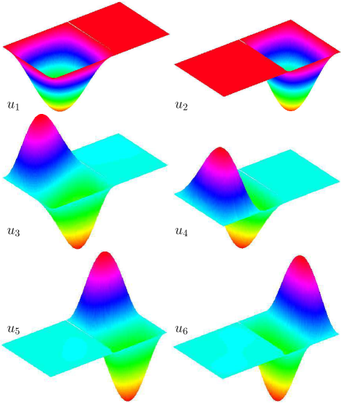
Fig. 5: The first six Dirichlet eigenfunctions in a rectangle with a vertical slit, $\Omega=([-a_{1},a_{2}]\times[0,1])\backslash(\{0\}\times[0,h])$, with $a_{1}=1$, $a_{2}=0.8$ and $h=0.1$. Eigenfunctions $u_{1}$, $u_{3}$, $u_{4}$ are localized in the larger domain $\Omega_{1}$ while $u_{2}$, $u_{5}$ and $u_{6}$ are localized in $\Omega_{2}$.

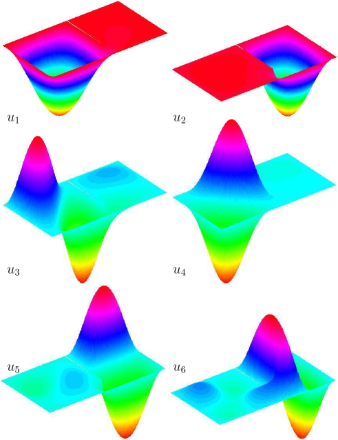
Fig. 6: The first six Dirichlet eigenfunctions in a rectangle with a slit, $\Omega=([-a_{1},a_{2}]\times[0,1])\backslash(\{0\}\times[0,h])$, with $a_{1}=1$, $a_{2}=0.8$ and $h=0.25$. Eigenfunctions $u_{1}$, $u_{3}$, $u_{4}$ are localized in the larger domain $\Omega_{1}$ while $u_{2}$, $u_{5}$ and $u_{6}$ are localized in $\Omega_{2}$.

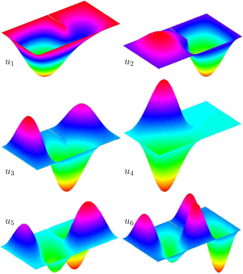
Fig. 7: The first six Dirichlet eigenfunctions in a rectangle with a slit, $\Omega=([-a_{1},a_{2}]\times[0,1])\backslash(\{0\}\times[0,h])$, with $a_{1}=1$, $a_{2}=0.8$ and $h=0.5$. Only eigenfunctions $u_{1}$ and $u_{4}$ remain localized.

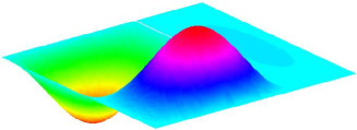
Fig. 8: The second Dirichlet eigenfunction in a rectangle with a vertical slit, $\Omega=([-a_{1},a_{2}]\times[0,1])\backslash(\{0\}\times[0,h])$, with $a_{1}=1$, $a_{2}=0.5$ and $h=0.1$. This eigenfunction is still localized in $\Omega_{1}$ although the condition (84) is not satisfied: $\sqrt{a_{2}^{2}(\nu_{2}-\nu_{1})/\pi^{2}+a_{2}^{2}/a_{1}^{2}}=1$, given that $\nu_{1}=\pi^{2}$ and $\nu_{2}=4\pi^{2}$.

Appendix B Proof of the classical lemma 1

Here we provide an elementary proof of the classical lemma 1.

Proof. Let $\lambda_{k}$ and $\psi_{k}$ denote eigenvalues and $L_{2}$-normalized eigenfunctions of $A$ forming a complete basis in $L_{2}$. Let us decompose $v$ on this basis: $v=\sum_{k}c_{k}\psi_{k}$. One has then

$$\|Av-\mu v\|^{2}_{L_{2}}=\biggl{\|}\sum\limits_{k}(\lambda_{k}-\mu)c_{k}\psi_{k}\biggr{\|}^{2}_{L_{2}}=\sum\limits_{k}(\lambda_{k}-\mu)^{2}c_{k}^{2}\geq\min\limits_{k}\{(\lambda_{k}-\mu)^{2}\}\sum\limits_{k}c_{k}^{2},$$ (142)

i.e.,

$$\|Av-\mu v\|_{L_{2}}\geq\min\limits_{k}\{|\lambda_{k}-\mu|\}~{}\|v\|_{L_{2}}.$$ (143)

On the other hand, (23) implies that

$$\min\limits_{k}\{|\lambda_{k}-\mu|\}<\varepsilon$$ (144)

that completes the proof. ∎

Appendix C Some inequalities involving Bessel functions

In this Appendix, we prove several inequalities involving Bessel functions. The technique of proofs is standard and can be found in classical textbooks [45, 46, 47].

Lemma 16.

If $\sqrt{\lambda}\,R_{1}\leq j^{\prime}_{1}$, then for any $\nu\geq 0$,

$$J_{\nu}(\sqrt{\lambda}\,r)>0\qquad\forall~{}0<r\leq R_{1},$$ (145)

where $j^{\prime}_{1}\approx 1.8412$ is the first zero of $J^{\prime}_{1}(z)$.

Proof. The known inequalities on the first zeros $j_{\nu}$ of Bessel functions $J_{\nu}(z)$,

$$j^{\prime}_{1}<j_{0}\leq j_{\nu}\qquad\forall~{}\nu\geq 0,$$ (146)

imply that $J_{\nu}(\sqrt{\lambda}\,r)$ does not change sign in the interval $(0,R_{1})$. In turn, the asymptotic behavior $J_{\nu}(x)\simeq(x/2)^{\nu}/\Gamma(\nu+1)$ as $x\to 0$ ensures the positive sign. ∎

Lemma 17.

If $\sqrt{\lambda}\,R_{1}\leq j^{\prime}_{1}$, then for any $0\leq\nu_{1}<\nu_{2}$, one has

$$\frac{J^{\prime}_{\nu_{1}}(\sqrt{\lambda}\,r)}{J_{\nu_{1}}(\sqrt{\lambda}\,r)}\leq\frac{J^{\prime}_{\nu_{2}}(\sqrt{\lambda}\,r)}{J_{\nu_{2}}(\sqrt{\lambda}\,r)}\qquad\forall~{}0<r\leq R_{1}.$$ (147)

Proof. Although the proof is standard, we provide it for completeness.

Writing the Bessel equations for $J_{\nu_{1}}(\sqrt{\lambda}\,r)$ and $J_{\nu_{2}}(\sqrt{\lambda}\,r)$,

$$\frac{1}{r}\frac{d}{dr}\left(r\frac{dJ_{\nu_{1}}(\sqrt{\lambda}\,r)}{dr}\right)+\lambda J_{\nu_{1}}(\sqrt{\lambda}\,r)-\frac{\nu_{1}^{2}}{r^{2}}J_{\nu_{1}}(\sqrt{\lambda}r) = 0,$$

$$\frac{1}{r}\frac{d}{dr}\left(r\frac{dJ_{\nu_{2}}(\sqrt{\lambda}\,r)}{dr}\right)+\lambda J_{\nu_{2}}(\sqrt{\lambda}\,r)-\frac{\nu_{2}^{2}}{r^{2}}J_{\nu_{2}}(\sqrt{\lambda}r) = 0,$$

multiplying the first one by $rJ_{\nu_{2}}(\sqrt{\lambda}\,r)$, the second one by $rJ_{\nu_{1}}(\sqrt{\lambda}\,r)$, and subtracting one from the other, one gets

$$\frac{d}{dr}r\left(J_{\nu_{1}}(\sqrt{\lambda}\,r)\frac{dJ_{\nu_{2}}(\sqrt{\lambda}\,r)}{dr}-J_{\nu_{2}}(\sqrt{\lambda}\,r)\frac{dJ_{\nu_{1}}(\sqrt{\lambda}\,r)}{dr}\right)$$

$$+\frac{\nu_{1}^{2}-\nu_{2}^{2}}{r}J_{\nu_{1}}(\sqrt{\lambda}\,r)J_{\nu_{2}}(\sqrt{\lambda}\,r)=0.$$ (148)

The integration from $0$ to $r$ yields

$$\sqrt{\lambda}r\left(J_{\nu_{1}}(\sqrt{\lambda}\,r)J^{\prime}_{\nu_{2}}(\sqrt{\lambda}\,r)-J_{\nu_{2}}(\sqrt{\lambda}\,r)J^{\prime}_{\nu_{1}}(\sqrt{\lambda}\,r)\right)$$

$$=\int\limits_{0}^{r}\frac{\nu_{2}^{2}-\nu_{1}^{2}}{r^{\prime}}J_{\nu_{1}}(\sqrt{\lambda}\,r^{\prime})J_{\nu_{2}}(\sqrt{\lambda}\,r^{\prime})dr^{\prime},$$ (149)

and the integral is strictly positive due to (145). ∎

Lemma 18.

If $\sqrt{\lambda}\,R_{1}\leq j^{\prime}_{1}$, then for any $\nu\geq 1$, one has

$$J^{\prime}_{\nu}(\sqrt{\lambda}\,r) \geq 0\hskip 61.17342pt\forall~{}0<r<R_{1},$$ (150)

$$J_{\nu}(\sqrt{\lambda}\,r) \leq J_{\nu}(\sqrt{\lambda}\,R_{1})\qquad\forall~{}0<r\leq R_{1},$$ (151)

$$\frac{J^{\prime}_{\nu}(\sqrt{\lambda}\,r)}{J_{\nu}(\sqrt{\lambda}\,r)} \geq 0\hskip 61.74246pt\forall~{}0<r\leq R_{1}.$$ (152)

Proof. The first inequality (150) is a direct consequence of Lemma 16, Lemma 17, and the inequality $J^{\prime}_{1}(\sqrt{\lambda}\,r)\geq 0$ which is fulfilled for $0<r<R_{1}$. The second inequality (151) follows from the first one. The third inequality (152) is a consequence of the first one and Lemma 16. ∎

Now we turn to the function $\psi_{n}(\sqrt{\lambda}\,r)$ defined by (111) which satisfies the Bessel equation:

$$\frac{1}{r}\frac{d}{dr}\left(r\frac{d\psi_{n}(\sqrt{\lambda}\,r)}{dr}\right)+\lambda\psi_{n}(\sqrt{\lambda}\,r)-\frac{\alpha_{n}^{2}}{r^{2}}\psi_{n}(\sqrt{\lambda}\,r)=0.$$ (153)

Lemma 19.

For any $0<a<b$, one has

$$\int\limits_{a}^{b}dr\,r\,\psi_{n}^{2}(\sqrt{\lambda}\,r)=\frac{1}{2\lambda}\left.\left((r\psi^{\prime}_{n}(\sqrt{\lambda}\,r))^{2}+(\lambda r^{2}-\alpha_{n}^{2})\psi_{n}^{2}(\sqrt{\lambda}\,r)\right)\right|_{r=a}^{r=b}.$$ (154)

Proof. The proof is obtained by multiplying the Bessel equation (153) by $r^{2}\psi^{\prime}_{n}$ and integrating from $a$ to $b$. ∎

Lemma 20.

If $\alpha_{n}^{2}/R_{2}^{2}>\lambda$, then

$$-\frac{\psi^{\prime}_{n}(\sqrt{\lambda}\,r)}{\psi_{n}(\sqrt{\lambda}\,r)}\geq\frac{r\,b(r)\,b(R_{2})}{\lambda^{3/2}+\sqrt{\lambda^{3}+r^{2}\,b(r)\,b^{2}(R_{2})}}\qquad\forall~{}0<r<R_{2},$$ (155)

where $b(r)=\alpha_{n}^{2}/r^{2}-\lambda$.

Proof. We introduce a new function $v(z)=\psi_{n}(\sqrt{\lambda}\,r)$ by changing the variable $z=\ln(r/\alpha_{n})$, with $r\in(0,R_{2})$. Starting from the Bessel equation for $\psi_{n}(\sqrt{\lambda}\,r)$, it is easy to check that the new function $v$ satisfies the equation

$$v^{\prime\prime}(z)=(1-\lambda e^{2z})\alpha^{2}_{n}v(z),$$ (156)

where prime denotes the derivative with respect to $z$. One has then

$$(v^{2})^{\prime\prime} = 2vv^{\prime\prime}+2(v^{\prime})^{2}\geq 2vv^{\prime\prime}=2\alpha^{2}_{n}(1-\lambda e^{2z})v^{2}$$ (157)

$$= 2\alpha^{2}_{n}\left(1-\lambda(r/\alpha_{n})^{2}\right)v^{2}\geq 2\alpha^{2}_{n}\left(1-\lambda(R_{2}/\alpha_{n})^{2}\right)v^{2}$$

$$= 2R_{2}^{2}\,b(R_{2})\,v^{2},$$

where we used $r<R_{2}$, and $b(R_{2})=\alpha_{n}^{2}/R_{2}^{2}-\lambda>0$. Integration of this inequality from $z$ to $z_{2}=\ln(R_{2}/\alpha_{n})$ yields

$$-2v^{\prime}v=-(v^{2})^{\prime}=\int\limits_{z}^{z_{2}}dz^{\prime}(v^{2})^{\prime\prime}\geq 2R_{2}^{2}\,b(R_{2})\int\limits_{z}^{z_{2}}dz^{\prime}v^{2}(z^{\prime}),$$ (158)

where $(v^{2})^{\prime}_{z=z_{2}}=2v^{\prime}(z_{2})v(z_{2})=0$ due to the boundary condition $\psi_{n}(\sqrt{\lambda}\,R_{2})=0$. One gets then

$$-\frac{v^{\prime}(z)}{v(z)}\geq\frac{R_{2}^{2}\,b(R_{2})}{v^{2}(z)}\int\limits_{z}^{z_{2}}dz^{\prime}v^{2}(z^{\prime}).$$ (159)

Since

$$\frac{d}{dr}\psi_{n}(\sqrt{\lambda}\,r)=\frac{dv}{dr}=\frac{dz}{dr}\frac{dv}{dz}=\frac{1}{r}v^{\prime},$$ (160)

one obtains

$$-\frac{\frac{d}{dr}\psi_{n}(\sqrt{\lambda}\,r)}{\psi_{n}(\sqrt{\lambda}\,r)}\geq\frac{R_{2}^{2}\,b(R_{2})}{r\psi_{n}^{2}(\sqrt{\lambda}\,r)}\int\limits_{r}^{R_{2}}\frac{dr^{\prime}}{r^{\prime}}\psi_{n}^{2}(\sqrt{\lambda}\,r^{\prime}).$$ (161)

We conclude that

$$-\frac{\psi^{\prime}_{n}(\sqrt{\lambda}\,r)}{\psi_{n}(\sqrt{\lambda}\,r)}>0.$$ (162)

One can further improve the lower bound. The integral in the right-hand side of (161) can be estimated as

$$\int\limits_{r}^{R_{2}}\frac{dr^{\prime}}{r^{\prime}}\psi_{n}^{2}(\sqrt{\lambda}\,r^{\prime}) = \int\limits_{r}^{R_{2}}\frac{dr^{\prime}}{r^{\prime 2}}r^{\prime}\psi_{n}^{2}(\sqrt{\lambda}\,r^{\prime})\geq\frac{1}{R_{2}^{2}}\int\limits_{r}^{R_{2}}dr^{\prime}\,r^{\prime}\,\psi_{n}^{2}(\sqrt{\lambda}\,r^{\prime})$$

$$= \frac{1}{R_{2}^{2}}\frac{1}{2\lambda}\left.\left((r^{\prime}\psi^{\prime}_{n}(\sqrt{\lambda}\,r^{\prime}))^{2}+(\lambda r^{\prime 2}-\alpha_{n}^{2})\psi_{n}^{2}(\sqrt{\lambda}\,r^{\prime})\right)\right|_{r^{\prime}=r}^{r^{\prime}=R_{2}}$$

$$= \frac{1}{2\lambda R_{2}^{2}}\left((R_{2}\psi^{\prime}_{n}(\sqrt{\lambda}\,R_{2}))^{2}-(r\psi^{\prime}_{n}(\sqrt{\lambda}\,r))^{2}+(\alpha_{n}^{2}-\lambda r^{2})\psi_{n}^{2}(\sqrt{\lambda}\,r)\right),$$

where we used (154) and the condition $\psi_{n}(\sqrt{\lambda}\,R_{2})=0$. We get then

$$\begin{split}-\frac{\psi^{\prime}_{n}(\sqrt{\lambda}\,r)}{\psi_{n}(\sqrt{\lambda}\,r)}&\geq\frac{b(R_{2})\,r}{2\lambda^{3/2}}\left(-\left(\frac{\psi^{\prime}_{n}(\sqrt{\lambda}\,r)}{\psi_{n}(\sqrt{\lambda}\,r)}\right)^{2}+b(r)\right),\\ \end{split}$$ (163)

where we dropped the positive term $(R_{2}\psi^{\prime}_{n}(\sqrt{\lambda}\,R_{2}))^{2}$. Denoting $w=-\frac{\psi^{\prime}_{n}(\sqrt{\lambda}\,r)}{\psi_{n}(\sqrt{\lambda}\,r)}$ and $a=rb(R_{2})/(2\lambda^{3/2})$, the above inequality can be written as

$$aw^{2}+w-ab(r)\geq 0.$$ (164)

Since $a>0$ and $w>0$, this inequality implies

$$-\frac{\psi^{\prime}_{n}(\sqrt{\lambda}\,r)}{\psi_{n}(\sqrt{\lambda}\,r)}\geq\frac{2ab(r)}{1+\sqrt{1+4a^{2}b(r)}}\qquad\forall~{}0<r<R_{2},$$ (165)

which is equivalent to (155). ∎

Corollary 21.

If $\alpha_{n}^{2}/R_{2}^{2}>\lambda$, then $\psi_{n}(\sqrt{\lambda}\,r)$ is a positive monotonously decreasing function on the interval $(0,R_{2})$:

$$\psi_{n}(\sqrt{\lambda}\,r)\geq 0,\qquad\psi^{\prime}_{n}(\sqrt{\lambda}\,r)\leq 0,\qquad\forall~{}0<r\leq R_{2}.$$ (166)

Proof. The inequality (162) implies that $\psi_{n}(\sqrt{\lambda}\,r)$ is either positive monotonously decreasing or negative monotonously increasing on the interval $(0,R_{2})$. We compute then

$$\psi^{\prime}_{n}(\sqrt{\lambda}\,R_{2})=J^{\prime}_{\alpha_{n}}(\sqrt{\lambda}\,R_{2})Y_{\alpha_{n}}(\sqrt{\lambda}\,R_{2})-Y^{\prime}_{\alpha_{n}}(\sqrt{\lambda}\,R_{2})J_{\alpha_{n}}(\sqrt{\lambda}\,R_{2})=-\frac{2}{\pi\sqrt{\lambda}\,R_{2}}<0,$$ (167)

where we used the Wronskian for Bessel functions. As a consequence, $\psi^{\prime}_{n}$ is negative in a vicinity of $R_{2}$ and thus on the whole interval. ∎

Corollary 22.

If $\lambda$ is fixed by (118), then there exists $\alpha_{1}$ large enough such that for any $n\geq 2$,

$$\psi_{n}(\sqrt{\lambda}\,r)\geq 0,\qquad\psi^{\prime}_{n}(\sqrt{\lambda}\,r)\leq 0,\qquad\forall~{}0<r\leq R_{2},$$ (168)

and

$$-\frac{\psi^{\prime}_{n}(\sqrt{\lambda}\,R_{1})}{\psi_{n}(\sqrt{\lambda}\,R_{1})}\geq-\frac{J^{\prime}_{0}(\sqrt{\lambda}\,R_{1})}{J_{0}(\sqrt{\lambda}\,R_{1})}.$$ (169)

Proof. When $\lambda$ is given by (118), one has

$$b(R_{2})=\frac{n^{2}\alpha_{1}^{2}}{R_{2}^{2}}-\lambda=c_{2}\lambda,\qquad c_{2}=\frac{n^{2}}{(1+\varepsilon_{1})^{2}}-1>0$$ (170)

and

$$b(R_{1})=\frac{n^{2}\alpha_{1}^{2}}{R_{1}^{2}}-\lambda=(R_{2}^{2}c_{1}-1)\lambda,\qquad c_{1}=\frac{n^{2}}{R_{1}^{2}(1+\varepsilon_{1})^{2}}>0$$ (171)

for any $n\geq 2$ and $\alpha_{1}$ large enough (that makes $\varepsilon_{1}$ small enough). As a consequence, Corollary 21 implies (168), while Lemma 20 implies

$$-\frac{\psi^{\prime}_{n}(\sqrt{\lambda}\,R_{1})}{\psi_{n}(\sqrt{\lambda}\,R_{1})}\geq\frac{R_{1}\,b(R_{1})\,b(R_{2})}{\lambda^{3/2}+\sqrt{\lambda^{3}+R_{1}^{2}\,b(R_{1})\,b^{2}(R_{2})}}=C_{n}R_{2},$$ (172)

with

$$C_{n}=\frac{R_{1}(c_{1}-1/R_{2}^{2})c_{2}\sqrt{\lambda}}{1/R_{2}+\sqrt{1/R_{2}^{2}+R_{1}^{2}(c_{1}-1/R_{2}^{2})c_{2}^{2}}}\longrightarrow\sqrt{c_{1}\lambda}\qquad\mbox{ as }R_{2}\to\infty.$$ (173)

In other words, when $\lambda$ is fixed by (118), the left-hand side of (172) can be made arbitrarily large. On the other hand, for a fixed $\lambda$, the term $\frac{J^{\prime}_{0}(\sqrt{\lambda}\,R_{1})}{J_{0}(\sqrt{\lambda}\,R_{1})}$ in the inequality (169) is independent of $\alpha_{1}$ or $R_{2}$. We conclude that the inequality (169) is fulfilled for $\alpha_{1}$ (and $R_{2}$) large enough. ∎

Lemma 23.

If $\lambda$ is fixed by (118), then there exists $\alpha_{1}$ large enough such that for any $n_{2}>n_{1}\geq 2$, one has

$$\frac{\psi^{\prime}_{n_{1}}(\sqrt{\lambda}\,r)}{\psi_{n_{1}}(\sqrt{\lambda}\,r)}\geq\frac{\psi^{\prime}_{n_{2}}(\sqrt{\lambda}\,r)}{\psi_{n_{2}}(\sqrt{\lambda}\,r)}\qquad\forall~{}0<r<R_{2}.$$ (174)

Proof. Integration of (148) from $r$ to $R_{2}$ yields

$$-r\left(\psi_{n_{1}}(\sqrt{\lambda}\,r)\psi^{\prime}_{n_{2}}(\sqrt{\lambda}\,r)-\psi_{n_{2}}(\sqrt{\lambda}\,r)\psi^{\prime}_{n_{1}}(\sqrt{\lambda}\,r)\right)$$

$$=\int\limits_{r}^{R_{2}}\frac{(\pi n_{2}/\phi_{1})^{2}-(\pi n_{1}/\phi_{1})^{2}}{r^{\prime}}\psi_{n_{1}}(\sqrt{\lambda}\,r^{\prime})\psi_{n_{2}}(\sqrt{\lambda}\,r^{\prime})dr^{\prime},$$ (175)

where the upper limit at $r=R_{2}$ vanished due to the boundary condition $\psi_{n}(\sqrt{\lambda}\,R_{2})=0$. Since $\psi_{n}(\sqrt{\lambda}\,r)\geq 0$ over $r\in(0,R_{2})$ according to (168), the integral is positive that implies (174). ∎

Note that the sign of inequality is opposite here as compared to the inequality (147).

References

- [1] R. Mittra and S. W. Lee, Analytical Techniques in the Theory of Guided Waves, New York, The Macmillan Company, 1971.
- [2] L. Levin, Theory of Waveguides: Techniques for the Solution of Waveguide Problems, London, Newnes-Butterworth, 1975.
- [3] N. Marcuvitz (ed.) Waveguide Handbook, MIT Radiation Laboratory Series, vol. 10, New York: McGraw Hill, 1951.
- [4] L. A. Weinstein, The Theory of Diffraction and the Factorization Method, Boulder CA: The Golem Press, 1969.
- [5] R. E. Collin, Field Theory of Guided Waves, Piscataway, NJ: IEEE Press, 1991.
- [6] A. L. Delitsyn, B.-T. Nguyen and D. S. Grebenkov, Trapped modes in finite quantum waveguides, Eur. Phys. J. B, 85 (2012), pp. 176.
- [7] D. S. Grebenkov and B.-T. Nguyen, Geometrical structure of Laplacian eigenfunctions, SIAM Rev., 55 (2013), pp. 601-667.
- [8] J. T. Beale, Scattering frequencies of resonators, Comm. Pure Appl. Math., 26 (1973), pp. 549-564.
- [9] S. Jimbo, The singularly perturbed domain and the characterization for the eigenfunctions with Neumann boundary conditions, J. Diff. Eq., 77 (1989), pp. 322-350.
- [10] R. Hempel, L. Seco, and B. Simon, The essential spectrum of Neumann Laplacians on some bounded singular domain, J. Funct. Anal., 102 (1991), pp. 448-483.
- [11] S. Jimbo and Y. Morita, Remarks on the behavior of certain eigenvalues on a singularly perturbed domain with several thin channels, Comm. Part. Diff. Eq., 17 (1992), pp. 523-552.
- [12] S. Jimbo, Perturbation formula of eigenvalues in a singularly perturbed domain, J. Math. Soc. Japan, 45 (1993), pp. 339-356.
- [13] R. Brown, P. D. Hislop, and A. Martinez, Eigenvalues and resonances for domains with tubes: Neumann boundary conditions, J. Diff. Eq., 115 (1995), pp. 458-476.
- [14] R. R. Gadyl’shin, Characteristic frequencies of bodies with thin spikes. I. Convergence and estimates, Math. Notes, 54 (1993), pp. 1192-1199.
- [15] R. R. Gadyl’shin, Characteristic frequencies of bodies with thin spikes. II. Asymptotics, Math. Notes, 55 (1994), pp. 14-23.
- [16] J. M. Arrieta, Neumann eigenvalue problems on exterior perturbations of the domain, J. Diff. Eq., 118 (1995), pp. 54-103.
- [17] J. M. Arrieta, Rates of eigenvalues on a dumbbell domain. Simple eigenvalue case, Trans. Amer. Math. Soc., 347 (1995), pp. 3503-3531.
- [18] G. Raugel, Dynamics of partial differential equations on thin domains, in Dynamical Systems (Montecatini Terme, 1994), Lecture Notes in Math. 1609, Springer, Berlin, 1995, pp. 208-315.
- [19] D. Daners, Dirichlet problems on varying domains, J. Diff. Eq., 188 (2003), pp. 591-624.
- [20] R. R. Gadyl’shin, On the eigenvalues of a dumbbell with a thin handle, Izv. Math., 69 (2005), pp. 265-329.
- [21] S. Jimbo and S. Kosugi, Spectra of domains with partial degeneration, J. Math. Sci. Univ. Tokyo, 16 (2009), pp. 269-414.
- [22] V. Felli and S. Terracini, Singularity of eigenfunctions at the junction of shrinking tubes, J. Diff. Eq., 255 (2013), pp. 633-700.
- [23] R. Melrose, Geometric Scattering Theory, Stanford Lectures, Cambridge University Press, Cambridge, UK, 1995.
- [24] B. Sapoval, T. Gobron and A. Margolina, Vibrations of fractal drums, Phys. Rev. Lett., 67 (1991), pp. 2974-2977.
- [25] C. Even, S. Russ, V. Repain, P. Pieranski and B. Sapoval, Localizations in Fractal Drums: An Experimental Study, Phys. Rev. Lett., 83 (1999), pp. 726-729.
- [26] S. Felix, M. Asch, M. Filoche and B. Sapoval, Localization and increased damping in irregular acoustic cavities, J. Sound. Vibr., 299 (2007), pp. 965-976.
- [27] S. M. Heilman and R. S. Strichartz, Localized Eigenfunctions: Here You See Them, There You Don’t, Notices Amer. Math. Soc., 57 (2010), pp. 624-629.
- [28] R. Parker, Resonance effects in wake shedding from parallel plates: calculation of resonance frequencies, J. Sound Vib., 5 (1967), pp. 330-343.
- [29] F. Ursell, Mathematical aspects of trapping modes in the theory of surface waves, J. Fluid Mech., 183 (1987), pp. 421-437.
- [30] F. Ursell, Trapped Modes in a Circular Cylindrical Acoustic Waveguide, Proc. R. Soc. Lond. A, 435 (1991), pp. 575-589.
- [31] D. V. Evans, Trapped acoustic modes, IMA J. Appl. Math., 49 (1992), pp. 45-60.
- [32] D. V. Evans, M. Levitin, D. Vassiliev, Existence theorems for trapped modes, J. Fluid Mech., 261 (1994), pp. 21-31.
- [33] P. Exner, P. Seba, M. Tater, and D. Vanek, Bound states and scattering in quantum waveguides coupled laterally through a boundary window, J. Math. Phys., 37 (1996), pp. 4867.
- [34] W. Bulla, F. Gesztesy, W. Renger, and B. Simon, Weakly coupled bound states in quantum waveguides, Proc. Amer. Math. Soc., 125 (1997), pp. 1487-1495.
- [35] C. M. Linton and P. McIver, Embedded trapped modes in water waves and acoustics, Wave Motion, 45 (2007), pp. 16-29.
- [36] S. Hein and W. Koch, Acoustic resonances and trapped modes in pipes and tunnels, J. Fluid Mech., 605 (2008), pp. 401-428.
- [37] V. A. Kondrat’ev, Boundary value problems for elliptic equations in domains with conical or angular points, Tr. Mosk. Mat. Obs., 16 (1967), pp. 209-292.
- [38] O. A. Ladyzhenskaya, The Boundary Value Problems of Mathematical Physics, Applied Mathematical Sciences, Vol. 49, Springer Science+Business Media, New York, 1985.
- [39] D. Gilbarg and N. S. Trudinger, Elliptic Partial Differential Equations of Second Order, Springer-Verlag, Berlin, 2001.
- [40] J. L. Lions and E. Magenes, Non-homogeneous Boundary value Problems and Applications, Springer-Verlag, Berlin, New York, 1972.
- [41] P. Grisvard, Elliptic Problems in Nonsmooth Domains, MSM 24, Pitman Advanced Publishing Program, 1985.
- [42] P. Grisvard, Singularities in Boundary Value Problems, RMA 22, Masson, Springer-Verlag, 1992.
- [43] A. L. Delitsyn, The Discrete Spectrum of the Laplace Operator in a Cylinder with Locally Perturbed Boundary, Diff. Equ., 40 (2004), pp. 207.
- [44] A. L. Delitsyn, B.-T. Nguyen and D. S. Grebenkov, Exponential decay of Laplacian eigenfunctions in domains with branches of variable cross-sectional profiles, Eur. Phys. J. B, 85 (2012), pp. 371.
- [45] G. N. Watson, A treatise on the theory of Bessel functions, Cambridge Mathematical Library 1995.
- [46] F. Bowman, Introduction to Bessel functions, 1st Ed., Dover Publications Inc., 1958.
- [47] M. Abramowitz and I. A. Stegun, Handbook of Mathematical Functions, Dover Publisher, New York, 1965.