Nonlinear reconstruction of redshift space distortions

Abstract

We apply nonlinear reconstruction to the dark matter density field in redshift space and solve for the nonlinear mapping from the initial Lagrangian position to the final redshift space position. The reconstructed anisotropic field inferred from the nonlinear displacement correlates with the linear initial conditions to much smaller scales than the redshift space density field. The number of linear modes in the density field is improved by a factor of $30$–$40$ after reconstruction. We thus expect this reconstruction approach to substantially expand the cosmological information including baryon acoustic oscillations and redshift space distortions for dense low-redshift large scale structure surveys including for example SDSS main sample, DESI BGS, and 21 cm intensity mapping surveys.

I Introduction

Measuring the three-dimensional large-scale structure of the Universe provides a powerful method to probe particle physics and cosmology. Precision measurements of baryon acoustic oscillations (BAO) and redshift space distortions (RSD) can constrain dark energy models and modified theories of gravity Alam et al. (2017); Beutler et al. (2017a); Ross et al. (2017); Vargas-Magaña et al. (2016); Beutler et al. (2017b); Grieb et al. (2017); Sánchez et al. (2017); Satpathy et al. (2017); Zhao et al. (2017). The ongoing and upcoming surveys are mapping large swaths of the visible Universe Alam et al. (2017); Bandura et al. (2014); Xu et al. (2015); DESI Collaboration et al. (2016); Takada et al. (2014). However, the precision of the measured cosmological parameters (e.g. the BAO scale and the growth rate) is usually limited by the strong non-Gaussianities of the nonlinear data, which prevent a simple mapping to the linear initial conditions which are predicted by cosmological theories. Therefore, to better extract cosmological information from an observed nonlinear map, it is crucial to understand the nonlinearities that make the observed signatures deviate from the theoretical predictions and how to reduce these nonlinearities in the nonlinear map to obtain better statistics.

Reconstruction methods have been developed to reverse the nonlinear degradation of the BAO signal Eisenstein et al. (2007a); Tassev and Zaldarriaga (2012a); Schmittfull et al. (2015); Obuljen et al. (2017). The current standard BAO reconstruction method uses a linear mapping to reduce the shift nonlinearities in the observed nonlinear field Eisenstein et al. (2007a). The linear method is successfully applied to galaxy surveys and improves the measurements of the BAO scale Padmanabhan et al. (2012); Anderson et al. (2012); Kazin et al. (2014); Anderson et al. (2014); Tojeiro et al. (2014); Ross et al. (2015); Beutler et al. (2017a); Ross et al. (2017). However, the density field reconstruction methods based on the linearized continuity equation only capture the shift terms from large-scale linear bulk flows Eisenstein et al. (2007b); Padmanabhan et al. (2009); Noh et al. (2009); Tassev and Zaldarriaga (2012b); Tassev (2014); Seo et al. (2016). Recently a new reconstruction method has been proposed in Ref. Zhu et al. (2017). (See also Refs. Schmittfull et al. (2017); Shi et al. (2018) for different implementations based on the same principle.) The new method solves a nonlinear bijective mapping between the Eulerian coordinate system and a new coordinate system, where the mass per volume element is constant Zhu et al. (2017). The nonlinear mapping provides a significantly better estimate of the nonlinear displacement compared to standard reconstruction. The linear density field inferred from the nonlinear bijective mapping gives a much better correlation with the linear initial conditions Zhu et al. (2017). These nonlinear methods are expected to substantially improve BAO measurements in the near future.

Most nonlinear reconstruction methods developed recently focus on improving measurements of the linear BAO signal Zhu et al. (2017); Schmittfull et al. (2017); Shi et al. (2018); Seljak et al. (2017). The current standard reconstruction also only works for reversing the nonlinear degradation of the BAO feature in galaxy redshift surveys, though different conventions for the RSD effect are adopted. (See Ref. Seo et al. (2016) for more discussions about different RSD conventions.) The RSD effect is also one of the most powerful probes of the Universe, complementary to the BAO measurements Jackson (1972); Sargent and Turner (1977); Peebles (1980); Kaiser (1987); Peacock and Dodds (1994); Ballinger et al. (1996). Precise measurements of the growth rate of structure from the RSD effect can provide tests of general relativity. While the distinct BAO feature can be measured easily, extracting information from RSD measurements requires the modeling of the power spectrum amplitude. Thus the analysis of RSD is often limited to much smaller wave numbers (e.g. $k<0.15\ h/\mathrm{Mpc}$ compared to $k<0.3\ h/\mathrm{Mpc}$ for the BAO-only analysis Beutler et al. (2017a, b)). A lot of effort has been made to model the nonlinear RSD effect Fisher (1995); Heavens et al. (1998); White (2001); Seljak (2001); Kang et al. (2002); Scoccimarro (2004); Tinker et al. (2006); Tinker (2007); Desjacques and Sheth (2010); Taruya et al. (2010); Matsubara (2011); Okumura and Jing (2011); Okamura et al. (2011); Sato and Matsubara (2011); Jennings et al. (2011); Reid and White (2011); Seljak and McDonald (2011); Okumura et al. (2012a, b); Kwan et al. (2012); Zhang et al. (2013); Zheng et al. (2013); Ishikawa et al. (2014); White et al. (2015); Bianchi et al. (2015, 2016); Jennings et al. (2016); Hand et al. (2017). However, even if the nonlinear RSD effect can be modeled to nonlinear scales, this still does not improve the power spectrum information content of a nonlinear map. Present RSD analysis is limited by the strong nonlinearities of the density and velocity fields and the nonlinear mapping from real to redshift space, with a small amount of cosmological information being extracted from galaxy surveys. Another possible way to handle the nonlinear RSD effect would be trying to reduce non-Gaussianities of the nonlinear density field in redshift space, in order to unscramble the cosmological information encoded in higher order statistics of the nonlinear data and increase the power spectrum information content of the reconstructed linear map.

In this paper, we apply nonlinear reconstruction to the dark matter density field in redshift space and solve for the nonlinear mapping from the initial Lagrangian position to the final redshift space position. The reconstructed anisotropic field inferred from the nonlinear displacement correlates with the linear initial conditions to much smaller scales than the redshift space density field. Therefore, we are able to significantly increase the constraining power of anisotropic galaxy clustering measurements by including small-scale density fluctuations in the analysis and provide tighter constraints on the structure growth rate. The idea of RSD reconstruction proposed here would be crucial for improving the RSD measurements from current and future galaxy surveys.

This paper is organized as follows. In Sec. II, we describe the motivation for reconstruction of RSD. Section III describes the performance tests of reconstruction and shows the reconstruction results. In Sec. IV, we describe some applications of reconstruction. We conclude in Sec. V. Appendix A shows the statistical properties of Lagrangian displacements. In Appendixes B and C, we present the study of Lagrangian velocities and shift velocities. Appendix D shows the RSD reconstruction results for halos. Appendix E describes how to implement nonlinear reconstruction in the presence of mask.

II Physical motivation

The Lagrangian space perturbation theories which capture the nonlinear shift terms provide a successful description of the matter distribution on large scales Matsubara (2008a, b, 2014); Porto et al. (2014); Carlson et al. (2013); Vlah et al. (2015a); Seljak and Vlah (2015); Vlah et al. (2015b, 2016); McQuinn and White (2016); Baldauf et al. (2016a, b). In the Lagrangian picture of structure formation, the Eulerian position $\bm{x}$ of each mass element is given by the sum of its initial Lagrangian coordinate $\bm{q}$ and the subsequent displacement $\bm{\psi}(\bm{q})$,

$$\bm{x}(\bm{q})=\bm{q}+\bm{\psi}(\bm{q}).$$ (1)

The displacement field which defines the mapping from initial Lagrangian coordinates to Eulerian coordinates is the key variable in Lagrangian space based perturbation theories. Since the initial density field is almost uniform, the nonlinear density at the Eulerian position $\bm{x}$ is

$$\rho(\bm{x})d^{3}x=\rho(\bm{q})d^{3}q,$$ (2)

where $\rho(\bm{q})\approx\mathrm{constant}$. The mass conservation equation predicts the exact nonlinear density $\rho(\bm{x})=d^{3}q/d^{3}x-1$ at $\bm{x}$ in the absence of shell crossing. Therefore, the key ingredient of Lagrangian perturbation theory calculation is to solve the nonlinear displacement field and calculate the Jacobian of the mapping from $\bm{q}$ to $\bm{x}$.

The redshift space position $\bm{s}$ of an object is shifted from its real space position $\bm{x}$ by its peculiar velocity,

$$\bm{s}(\bm{x})=\bm{x}+\frac{v_{z}(\bm{x})}{aH}\hat{z},$$ (3)

where $a$ is the scale factor and $H$ is the Hubble parameter. In this paper we adopt the plane-parallel approximation and take the line of sight direction to be the $z$-axis. The density field in redshift space can be obtained by imposing mass conservation,

$$\rho(\bm{s})d^{3}s=\rho(\bm{x})d^{3}x.$$ (4)

Since the growth of displacement $\bm{\psi}(\bm{q})$ is the Lagrangian velocity $\bm{v}(\bm{q})$, the Eulerian velocity $\bm{v}(\bm{x})$ of a mass element at $\bm{x}=\bm{q}+\bm{\psi}(\bm{q})$ is simply the Lagrangian velocity $\bm{v}(\bm{q})$. Thus we can define a mapping from the initial Lagrangian coordinates $\bm{q}$ to the redshift space coordinates $\bm{s}$ as

$$\bm{s}(\bm{q})=\bm{q}+\bm{\psi}^{s}(\bm{q}),$$ (5)

where

$$\bm{\psi}^{s}(\bm{q})=\bm{\psi}(\bm{q})+{\bm{v}^{s}(\bm{q})}/{aH}.$$ (6)

Here $\bm{v}^{s}(\bm{q})\equiv[\hat{z}\cdot\bm{v}(\bm{q})]\hat{z}$ is called the shift velocity. The redshift space nonlinear density field is given by

$$\rho(\bm{s})d^{3}s=\rho(\bm{q})d^{3}q.$$ (7)

Again the nonlinear density at $\bm{s}$ predicted by Eq. (7) with the redshift space displacement field $\bm{\psi}^{s}(\bm{q})$ is exact before shell crossing happens.

The nonlinear mapping from real to redshift space has been studied extensively, which is necessary for modeling the nonlinear RSD effect. A successful nonlinear RSD model can reduce theoretical systematics in the analysis. However, the cosmological information extracted from redshift space two-point statistics is still limited by the shift nonlinearities in the observed density field. In order to remove the nonlinear shift terms induced by the mapping from $\bm{q}$ to $\bm{x}$ and then from $\bm{x}$ to $\bm{s}$, we can try to invert the nonlinear mapping and solve for the Lagrangian displacement and the shift velocity, which are Lagrangian quantities that are not affected by shift terms.

The basic idea of nonlinear reconstruction is to build a bijective mapping between the redshift space coordinates $\bm{s}$ and the potential isobaric coordinates $\bm{\xi}$, where $\rho(\bm{\xi})d^{3}\xi$ is approximately constant. We define a coordinate transformation that is a pure gradient,

$$s^{i}=\xi^{\mu}\delta^{i}_{\mu}+\frac{\partial\phi^{s}}{\partial\xi^{\nu}}\delta^{i\nu},$$ (8)

where $\phi^{s}(\bm{\xi})$ is the displacement potential. The potential isobaric gauge is unique as long as we require that the coordinate transformation defined above is positive definite, i.e., $\mathrm{det}(\partial s^{i}/\partial\xi^{\alpha})>0$. It becomes analogous to synchronous gauge and Lagrangian coordinates before shell crossing, but allows a unique mapping even after shell crossing. The unique displacement potential $\phi^{s}(\bm{\xi})$ consistent with the nonlinear density and positive definite coordinate transformation can be solved using the moving mesh approach, which evolves the coordinate system towards a state of constant mass per volume element, i.e., $\rho(\bm{\xi})d^{3}\xi=\mathrm{constant}$ Pen (1995, 1998). See Ref. Zhu et al. (2017) for the details of this calculation.

The gradient of the reconstructed displacement potential $\nabla_{\bm{\xi}}\phi^{s}(\bm{\xi})$ provides an estimate of the redshift space displacement $\bm{\psi}^{s}(\bm{q})$. We define the negative Laplacian of the reconstructed displacement potential as the reconstructed density field,

$$\delta_{r}^{s}(\bm{\xi})=-\nabla_{\bm{\xi}}\cdot\nabla_{\bm{\xi}}\phi^{s}(\bm{\xi})=-\nabla^{2}_{\bm{\xi}}\phi^{s}(\bm{\xi}).$$ (9)

Note that the reconstructed density field is computed on the potential isobaric coordinates instead of the redshift space coordinates.

Because of the limited degrees of freedom, we can only solve the scalar part of the nonlinear mapping, while the real nonlinear displacement also includes the curl part. The gradient and curl parts of the redshift space nonlinear displacement are

$$\bm{\psi}^{s}_{E}(\bm{q})=\bm{\psi}_{E}(\bm{q})+{\bm{v}^{s}_{E}(\bm{q})}/{aH},$$ (10)

and

$$\bm{\psi}^{s}_{B}(\bm{q})=\bm{\psi}_{B}(\bm{q})+{\bm{v}^{s}_{B}(\bm{q})}/{aH},$$ (11)

respectively, where

$$\bm{\psi}_{E}(\bm{k})=[\bm{k}\cdot\bm{\psi}(\bm{k})]\bm{k}/k^{2},\ \bm{\psi}_{B}(\bm{k})=\bm{\psi}(\bm{k})-\bm{\psi}_{E}(\bm{k}),$$ (12)

and

$$\bm{v}^{s}_{E}(\bm{k})=[\bm{k}\cdot\bm{v}^{s}(\bm{k})]\bm{k}/k^{2},\ \bm{v}_{B}^{s}(\bm{k})=\bm{v}^{s}(\bm{k})-\bm{v}^{s}_{E}(\bm{k}).$$ (13)

Since the displacement field is anisotropic in the presence of redshift space distortions, the reconstructed displacement potential is also anisotropic. In addition to the real space $E$-mode displacement $\bm{\psi}_{E}(\bm{q})$, the solved displacement also contains the $E$-mode shift velocity $\bm{v}_{E}^{s}(\bm{q})/aH$. The shift velocity is the most important observable in the RSD measurements since it describes the growth of the displacement, which provides cosmological information about the logarithmic growth rate $f=d\mathrm{ln}D/d\mathrm{ln}a$, where $D$ is the linear growth factor. This is new to all previous reconstruction algorithms since it is about reconstruction of the redshift space distortions.

Notice that the shift velocity $\bm{v}^{s}(\bm{q})$ is different from $\bm{v}(\bm{q})$, where the former corresponds to the $z$-component of the latter. The Lagrangian velocities $\bm{v}_{E}$ and $\bm{v}_{B}$ describe the growth of the Lagrangian displacements $\bm{\psi}_{E}$ and $\bm{\psi}_{B}$, respectively. The statistical properties of the Lagrangian displacements have been studied in Appendix A, while the Lagrangian and shift velocities have been investigated in Appendixes B and C.

III Performance tests

To test the performance of reconstruction with redshift space density field, we use a set of ten $N$-body simulations run with the ${\tt CUBEP^{3}M}$ code Harnois-Déraps et al. (2013). These simulations evolve $1024^{3}$ dark matter particles in a cubic box of length $600\ \mathrm{Mpc}/h$. We take the snapshot at redshift $z=0$ and compute the density on a $512^{3}$ grid. We solve the displacement potential $\phi^{s}$ using the multigrid algorithm and then compute the reconstructed density field using Eq. (9) in the potential isobaric gauge Zhu et al. (2017).

To check convergence of the reconstruction results, we run a high-resolution simulation of $2048^{3}$ particles with the same box size. We also perform reconstruction with the redshift space density field on a $512^{3}$ grid from the high-resolution simulation. We find that the reconstruction results with different simulation resolutions are almost indistinguishable. Therefore, we use the high-resolution simulation for visual comparison due to its better image resolution and use the statistical averaged power spectra from the other ten simulations to reduce statistical errors.

In the following subsections, we assess the performance of reconstruction in redshift space in terms of the density field slice, the correlation with the initial conditions, the correlation with the nonlinear field, the shape of the power spectrum, and the correlation with the Lagrangian displacements and velocities.

III.1 Nonlinear map with potential isobaric gauge

Figure 1 shows a slice of the nonlinear density through the high-resolution simulation, while the corresponding redshift space density field is presented in Fig. 2. We also plot the Eulerian positions of a uniform grid of potential isobaric coordinates on the corresponding density field slice. At small scales the random velocity dispersion elongates cosmic structures along the line of sight, leading to the finger of God effect. The finger of God effect smoothes the density fluctuations along the line of sight, blurring the clear small-scale structure in real space. This causes the loss of cosmological information about the initial conditions. Thus we expect that the performance in redshift space will be degraded compared to the result in real space.

The grid lines become closer in the higher density regions and sparser in the lower density regions. As a result, the mass enclosed in each curvilinear grid cell is approximately constant. Since the structure in redshift space is blurred along the line of sight, the grid lines also move apart in the dense regions compared to the corresponding real space grid line separation. This suppresses the small-scale power of the reconstructed density field along the line of sight. As the reconstructed density field is given by

$$\delta_{r}^{s}(\bm{\xi})=-\nabla_{\bm{\xi}}\cdot(\bm{s}(\bm{\xi})-\bm{\xi})=3-\nabla_{\bm{\xi}}\cdot\bm{s}(\bm{\xi}),$$ (14)

where $\nabla_{\bm{\xi}}\cdot\bm{s}(\bm{\xi})=\partial s_{x}/\partial\xi_{x}+\partial s_{y}/\partial\xi_{y}+\partial s_{z}/\partial\xi_{z}$, a larger separation $\Delta s_{z}$ between neighboring curvilinear grid lines implies a smaller density. Although the squashing effect on large scales is not obvious in the density field slice presented here, we still expect that the reconstructed density field will have similar statistical properties as the redshift space nonlinear densiy field but with much fewer nonlinearities.

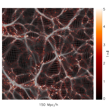
Figure 1: A slice of the nonlinear density field from the high-resolution simulation without the RSD effect. The curvilinear grid shows the Eulerian coordinate of each grid point of the potential isobaric coordinate.

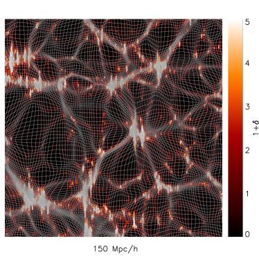
Figure 2: A slice of the nonlinear density field from the high-resolution simulation with the RSD effect. The curvilinear grid shows the Eulerian coordinate of each grid point of the potential isobaric coordinate.

III.2 Correlation with the linear initial conditions

To directly measure the linear initial conditions recovered with nonlinear reconstruction, we calculate the cross-correlation coefficient between the density field and the linear initial conditions. The power spectra used for computing the cross correlation coefficients are averaged over ten simulations to reduce the cosmic variance.

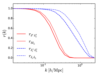
Figure 3: The cross-correlation coefficients with the initial conditions for the redshift space nonlinear (thick solid line) and reconstructed (thick dashed line) density fields and the nonlinear (thin sold line) and reconstructed (thin dashed line) density fields without redshift space distortions. The correlation with the linear field for the redshift space field after reconstruction is better than $50\%$ at $k\lesssim 0.6\ h/\mathrm{Mpc}$ and $80\%$ at $k\lesssim 0.3\ h/\mathrm{Mpc}$.

We correlate the nonlinear density field $\delta(\bm{k})$ and the reconstructed density field $\delta_{r}(\bm{k})$ in real space with the linear density $\delta_{L}(\bm{k})$. For the redshift space density field $\delta^{s}(\bm{k})$ and the reconstructed density field $\delta_{r}^{s}(\bm{k})$, we instead correlate them with the linear redshift space displacement divergence,

$$\delta^{s}_{L}(\bm{k})=-i\bm{k}\cdot\bm{\psi}^{s}_{L}(\bm{k})=(1+f\mu^{2})\delta_{L}(\bm{k}),$$ (15)

where $\mu=k_{z}/k$. To evaluate the overall performance, we first average the power spectrum over different directions and then compute the cross-correlation coefficient, i.e., the cross-correlation coefficient for the power spectrum monopole. Figure 3 shows the correlation of the redshift space density field with the linear initial conditions before and after nonlinear reconstruction. We also plot the cross-correlation coefficients for real space density fields for comparison. The correlation with the linear field for the redshift space field after reconstruction is better than $50\%$ at $k\lesssim 0.6\ h/\mathrm{Mpc}$ and $80\%$ at $k\lesssim 0.3\ h/\mathrm{Mpc}$. For the redshift space nonlinear density field, the correlation is better than $50\%$ and $80\%$ only at $k\lesssim 0.17\ h/\mathrm{Mpc}$ and $k\lesssim 0.1\ h/\mathrm{Mpc}$. Nonlinear reconstruction significantly reduces the shift nonlinearities and improves the number of linear modes by a factor $30$–$40$ depending on the scale used for comparison.

We note that RSD significantly degrade the performance of reconstruction. However, the nonlinear density field is less affected by RSD; the correlation with the linear density field is only slightly smaller than without RSD. This is because RSD mainly scramble small-scale nonlinear structures and these small-scale structures have almost no correlation with the initial conditions. However, we can recover the cosmological information which is still present in these structures. While RSD blur these visible small-scale structures, we can no longer recover the cosmological information that is present in the small-scale fluctuations of the real space density field.

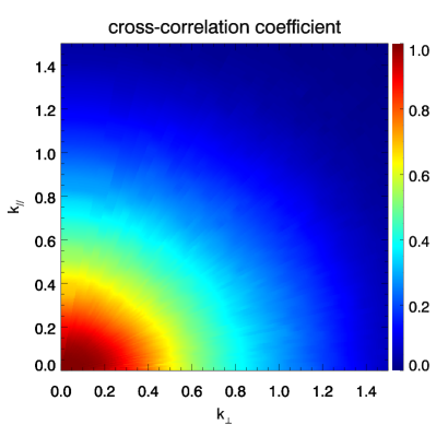
Figure 4: The two-dimensional cross-correlation coefficient of the reconstructed density field $\delta_{r}^{s}(\bm{k})$ with the redshift space linear field $\delta_{L}^{s}(\bm{k})=(1+f\mu^{2})\delta_{L}(\bm{k})$.

As the solved displacement potential is anisotropic in the presence of RSD, we expect that the performance of reconstruction will depend on the direction. Figure 4 shows the two-dimensional correlation coefficient $r_{\delta_{r}^{s}\delta_{L}^{s}}(k_{\perp},k_{\parallel})$ between the redshift space reconstructed density field and the linear density field. We also plot the correlation coefficients for three different $\mu$ bins, $\mu=0,0.5,1$, in Fig. 6. Note that the correlation with the linear field along the $k_{\parallel}$ axis drops faster than along the $k_{\perp}$ axis. One reason for this is that the Lagrangian velocity $\bm{v}(\bm{q})$ is much more nonlinear than the Lagrangian displacement $\bm{\psi}(\bm{q})$. The Lagrangian displacement is an integral of the Lagrangian velocity with respect to time,

$$\bm{\psi}(\bm{q},t)=\int_{0}^{t}\bm{v}(\bm{q},t^{\prime})/a(t^{\prime})dt^{\prime}.$$ (16)

At higher redshifts the velocity field is more linear than the velocity field at later time. The Lagrangian displacement is a linear combination of velocities at different redshifts with a different amount of nonlinearities, while the present-day Lagrangian velocity corresponds to the most nonlinear contribution to the displacement. More details about this are presented in Appendixes A and B. Since the combination of $\nabla\cdot\bm{\psi}$ and $\nabla\cdot\bm{v}^{s}/aH$ is more nonlinear than $\nabla\cdot\bm{\psi}$ and most power of $\nabla\cdot\bm{v}^{s}$ is concentrated in $\mu$ bins close to $\mu=1$, the correlation with the linear density field drops faster in these $\mu$ bins.

III.3 Correlation with the nonlinear field

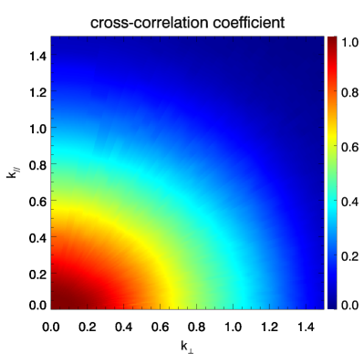
Figure 5: The two-dimensional cross-correlation coefficient of the reconstructed density field $\delta_{r}^{s}(\bm{k})$ with the redshift space nonlinear field $\delta_{E}^{s}(\bm{k})=-i\bm{k}\cdot(\bm{\psi}+\bm{v}^{s}/aH)(\bm{k})$.

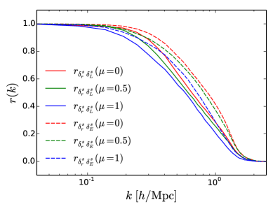
Figure 6: The correlation coefficients of the reconstructed density field $\delta_{r}^{s}(\bm{k})$ with the redshift space linear field $\delta_{L}^{s}(\bm{k})$ (solid lines) and the redshift space nonlinear field $\delta_{E}^{s}(\bm{k})$ (dashed lines) for three $\mu$ bins, $\mu=0,0.5,1$ (from right to left).

The correlation with the linear field quantifies the linear signal recovered with nonlinear reconstruction, which is relevant for improving the measurements of BAO scale in redshift surveys. To answer how well we reconstruct the nonlinear displacement, we need to correlate the reconstructed density field with the redshift space nonlinear displacement divergence,

$$\delta_{E}^{s}(\bm{k})=-i\bm{k}\cdot\bm{\psi}^{s}(\bm{k})=-i\bm{k}\cdot(\bm{\psi}+\bm{v}^{s}/aH)(\bm{k}).$$ (17)

Figure 5 demonstrates the two-dimensional correlation coefficient $r_{\delta_{r}^{s}\delta_{E}^{s}}(k_{\perp},k_{\parallel})$ between the redshift space reconstructed density field and the redshift space nonlinear $E$-mode displacement. We also plot the correlation coefficients for three different $\mu$ bins, $\mu=0,0.5,1$, in Fig. 6. The correlation with this nonlinear displacement field is much better than that with the linear displacement field as expected. The redshift space nonlinear displacement divergence represents the best possible theoretical description of the reconstructed density field.

We find that the cross-correlation coefficient with the nonlinear field shows similar anisotropic feature as the cross-correlation coefficient with the linear field. This is because our reconstruction method cannot recover the $B$-mode displacement $\bm{\psi}_{B}+\bm{v}_{B}^{s}/aH$. The $B$-mode real space nonlinear displacement $\bm{\psi}_{B}$ is negligible on scales we care about. The $x$- and $y$-components of the $B$-mode shift velocity $\bm{v}^{s}_{B}$ are also negligible. However, the $z$-component of the $B$-mode shift velocity $\bm{v}^{s}_{B}$ contributes $8/35$ of the total power of $\bm{v}^{s}$ on large scales and even more on smaller scales (see Appendix C). Therefore, the correlation with the nonlinear field is slightly lower in the $\mu$ bins close to $\mu=1$ as shown in Fig. 5. The effect may also cause part of the degradation of the correlation coefficient with the linear field along the line of sight.

III.4 Reconstruction with transfer functions

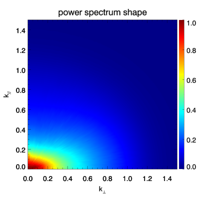
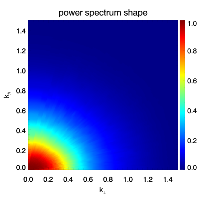
Figure 7: Top: The shape of the power spectrum for the reconstructed density field normalized to the linear field, defined as $P_{\delta_{r}^{s}}(\bm{k})/P_{\delta_{L}^{s}}(\bm{k})$. Bottom: The shape of the power spectrum for the filtered reconstructed density field normalized to the linear field, defined as $P_{\tilde{\delta}_{r}^{s}}(\bm{k})/P_{\delta_{L}^{s}}(\bm{k})$, where $\tilde{\delta}_{r}^{s}(\bm{k})=t_{L}(\bm{k})\delta_{r}^{s}(\bm{k})$.

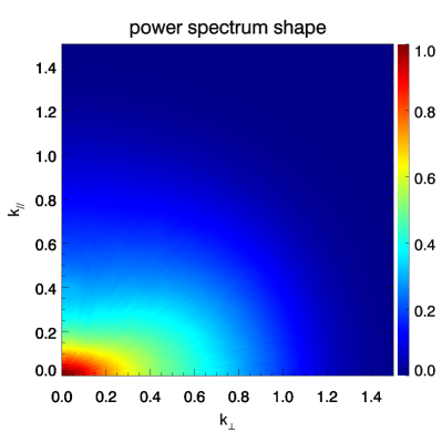
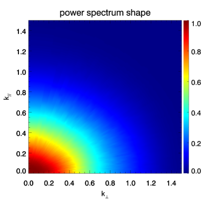
Figure 8: Top: The shape of the power spectrum for the reconstructed density field normalized to the nonlinear field, defined as $P_{\delta_{r}^{s}}(\bm{k})/P_{\delta_{E}^{s}}(\bm{k})$. Bottom: The shape of the power spectrum for the filtered reconstructed density field normalized to the nonlinear field, defined as $P_{\tilde{\delta}_{r}^{s}}(\bm{k})/P_{\delta_{E}^{s}}(\bm{k})$, where $\tilde{\delta}_{r}^{s}(\bm{k})=t_{E}(\bm{k})\delta_{r}^{s}(\bm{k})$.

To recover the broadband power of the reconstructed density field, we can use the transfer functions Schmittfull et al. (2017). We write the filtered reconstructed field as

$$\tilde{\delta}_{r}^{s}(\bm{k})=t(\bm{k})\delta_{r}^{s}(\bm{k}),$$ (18)

where $t(\bm{k})$ is the transfer function to be specified. Note that the transfer function is anisotropic in the presence of RSD. Here we consider the linear relation between different density fields and neglect the higher order correlations. We can choose the transfer function to minimize the difference between the reconstructed density field and the linear density field,

$$\langle(t(\bm{k}){\delta}_{r}^{s}(\bm{k})-\delta_{L}^{s}(\bm{k}))^{2}\rangle,$$ (19)

and then the linear transfer function is given by

$$t_{L}(\bm{k})=\frac{P_{\delta_{r}^{s}\delta_{L}^{s}}(\bm{k})}{P_{\delta_{r}^{s}}(\bm{k})},$$ (20)

where the subscript $L$ denoting the transfer function is to recover the broadband power of the reconstructed density field with respect to the linear field. We can also choose the transfer function to minimize the difference with respect to the nonlinear field,

$$\langle(t(\bm{k})\delta_{r}^{s}(\bm{k})-\delta_{E}^{s}(\bm{k}))^{2}\rangle,$$ (21)

and then the nonlinear transfer function is given by

$$t_{E}(\bm{k})=\frac{P_{\delta_{r}^{s}\delta_{E}^{s}}(\bm{k})}{P_{\delta_{r}^{s}}(\bm{k})},$$ (22)

where the subscript $E$ denoting the transfer function recovers the broadband power spectrum with respect to the nonlinear field.

Figure 7 shows the power spectra of the original and linear transfer function filtered reconstructed field, both normalized to the linear power spectrum. The linear transfer function significantly improves the matching of the power spectrum of the reconstructed field to the linear power spectrum. For reconstruction with transfer function, the ratio between the two power spectra is larger than $0.5$ at $k\lesssim 0.5\ h/\mathrm{Mpc}$ for $\mu$ bins around $\mu=0$ and $k\lesssim 0.4\ h/\mathrm{Mpc}$ for $\mu$ bins around $\mu=1$. Again, we note a deficit in power along the line of sight direction. This is because the shift velocity divergence $\nabla\cdot\bm{v}^{s}$ is more nonlinear than displacement and the reconstruction misses the $B$-mode shift velocity $\bm{v}^{s}_{B}$ as we have discussed above.

Figure 8 shows the power spectra of the original and nonlinear transfer function filtered reconstructed field, both normalized to the nonlinear power spectrum. The nonlinear transfer function significantly improves the matching of the power spectrum of the reconstructed field to the nonlinear power spectrum. For reconstruction with transfer function, the ratio between the two power spectra is larger than $0.5$ at $k\lesssim 0.6\ h/\mathrm{Mpc}$ for $\mu$ bins around $\mu\sim 0$ and $k\lesssim 0.5\ h/\mathrm{Mpc}$ for $\mu$ bins around $\mu\sim 1$. Here the missed power along the line of sight is solely due to the missed $B$-mode shift velocity $\bm{v}^{s}_{B}$.

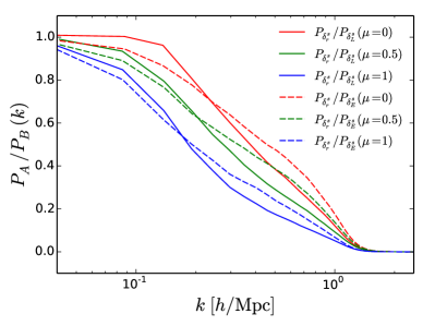
Figure 9: The reconstructed power spectrum divided by the linear (solid lines) and nonlinear (dashed) power spectra for three $\mu$ bins, $\mu=0,0.5,1$ (from right to left).

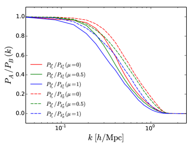
Figure 10: Same as Fig. 9 but for the linear/nonlinear transfer function filtered reconstructed density fields. The solid lines show results for the reconstructed density field filtered with the linear transfer function, i.e., $\tilde{\delta}_{r}^{s}(\bm{k})=t_{L}(\bm{k})\delta_{r}^{s}(\bm{k})$, while the dashed lines show the result with the nonlinear transfer function, i.e., $\tilde{\delta}_{r}^{s}(\bm{k})=t_{E}(\bm{k})\delta_{r}^{s}(\bm{k})$.

In Fig. 9, we plot the reconstructed power spectrum divided by the linear and nonlinear power spectra for three $\mu$ bins, $\mu=0,0.5,1$. We also present the corresponding results for the linear/nonlinear transfer function filtered fields in Fig. 10. We notice that on relative large scales $k\lesssim 0.1\ h/\mathrm{Mpc}$, the power spectrum amplitude ratio drops much faster than the correlation coefficient, which is also observed in other reconstruction methods Schmittfull et al. (2017); Seljak et al. (2017). Recovering the cross correlation is easier than the full broadband power spectrum. This problem can be solved by using the transfer function as we indeed observe in Fig. 10.

The transfer function introduced above is similar to the Wiener filter. The reconstructed density field can be written as

$$\delta_{r}^{s}(\bm{k})=C_{L}(\bm{k})\delta_{L}^{s}(\bm{k})+N_{L}(\bm{k}),$$ (23)

where $C_{L}(\bm{k})=P_{\delta_{r}^{s}\delta_{L}^{s}}(\bm{k})/P_{\delta_{L}^{s}}(\bm{k})$ is the propagator and $N_{L}(\bm{k})$ is the noise with respect to the linear field. The Wiener filter for the linear signal in reconstructed density field is

$$W_{L}(\bm{k})=\frac{C^{2}_{L}(\bm{k})P_{\delta_{L}^{s}}(\bm{k})}{C_{L}^{2}(\bm{k})P_{\delta^{s}_{L}}(\bm{k})+P_{N_{L}}(\bm{k})},$$ (24)

which differs from the linear transfer function $t_{L}(\bm{k})$ by a propagator $C_{L}(\bm{k})$,

$$t_{L}(\bm{k})=\frac{W_{L}(\bm{k})}{C_{L}(\bm{k})}.$$ (25)

The transfer function also deconvolves the propagator from the density field in addition to applying the Wiener filter to recover the power spectrum shape. Figure 11 shows the two-dimensional propagator with respect to the linear field. We also plot the propagator with respect to the linear field for three $\mu$ bins, $\mu=0,0.5,1$, in Fig. 13. The propagator shows additional suppression along the $z$-direction. This is caused by the nonlinearity of the shift velocity $\bm{v}^{s}$ and the finger of God effect. Since the combination of displacement divergence $\nabla\cdot\bm{\psi}$ and velocity divergence $\nabla\cdot\bm{v}^{s}$ is more nonlinear than $\nabla\cdot\bm{\psi}$ itself and most power of the shift velocity divergence $\nabla\cdot\bm{v}^{s}$ is concentrated around $\mu\sim 1$, the $\mu$ bins close to $\mu=1$ contain less information about the linear initial conditions. The small-scale random velocity dispersion suppresses the density fluctuations along the line of sight, leading to larger separations along the $z$-axis between neighboring grid lines. The nonlinear effects due to random motion on small scales not only cause the suppression of power along the line of sight, but also scramble the information about linear initial conditions along this direction.

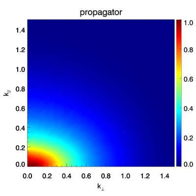
Figure 11: The propagator $C_{L}(\bm{k})$ for the linear field. The additional damping along the line of sight is caused by the nonlinearity of the shift velocity and the finger of God effect.

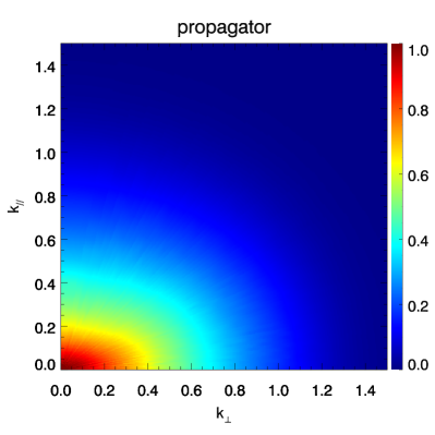
Figure 12: The propagator $C_{E}(\bm{k})$ for the nonlinear field. The additional damping along the line of sight is caused by the finger of God effect only as we are correlating with the nonlinear field.

We can also write the reconstructed density field as

$$\delta_{r}^{s}(\bm{k})=C_{E}(\bm{k})\delta_{E}^{s}(\bm{k})+N_{E}(\bm{k}),$$ (26)

where $C_{E}(\bm{k})=P_{\delta_{r}^{s}\delta_{E}^{s}(\bm{k})}/P_{\delta_{E}^{s}}(\bm{k})$ and $N_{E}(\bm{k})$ are the propagator and noise with respect to the nonlinear field. The similar relation $t_{E}(\bm{k})={W_{E}(\bm{k})}/{C_{E}(\bm{k})}$ also holds for the Wiener filter for the nonlinear signal

$$W_{E}(\bm{k})=\frac{C^{2}_{E}(\bm{k})P_{\delta_{E}^{s}}(\bm{k})}{C_{E}^{2}(\bm{k})P_{\delta^{s}_{E}}(\bm{k})+P_{N_{E}}(\bm{k})}.$$ (27)

Figure 12 shows the two-dimensional propagator with respect to the nonlinear field. We also plot the propagator with respect to the nonlinear field for three $\mu$ bins, $\mu=0,0.5,1$ in Fig. 13. Here the additional damping along the line of sight is only due to the Finger of God effect as we are correlating with the nonlinear field.

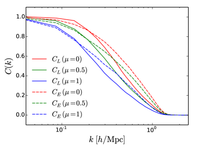
Figure 13: The linear propagator $C_{L}(\bm{k})$ (solid lines) and the nonlinear propagator $C_{E}(\bm{k})$ (dashed lines) for three $\mu$ bins, $\mu=0,0.5,1$ (from right to left).

To extract distinct features like BAO wiggles from the power spectrum of the reconstructed density field, we can directly apply the transfer function calibrated from simulations or mocks. In the BAO-only analysis, the transfer function is only used to match the power spectrum amplitude with the linear density field and itself does not contain any information about the BAO wiggles if calibrated to simulations with no-wiggle initial linear power spectra Schmittfull et al. (2017). However, if we want to extract additional cosmological information about RSD from the density field, we need to model the broadband power spectrum of the reconstructed density field. The linear power spectrum $P_{\delta_{L}^{s}}(\bm{k})$ or the nonlinear power $P_{\delta_{E}^{s}}(\bm{k})$ does not suffice to model the reconstructed density field, as they only describe the coherent part of the reconstructed density field. We need to consider the small-scale random velocity dispersion and the errors of reconstruction, i.e., the propagator $C(\bm{k})$ and the noise term $P_{N}(\bm{k})$. For the linear field, we also need to consider nonlinearities of the coherent part of the reconstructed field for modeling the mode-coupling term $P_{N}(\bm{k})$. Probably these can be studied using higher order Lagrangian perturbation theories or the effective field theories of large-scale structure Baldauf et al. (2016a). Similar works for the standard reconstruction method have been conducted Padmanabhan et al. (2009); Noh et al. (2009); Schmittfull et al. (2015); White (2015); Seo et al. (2016); Hikage et al. (2017). We can directly calibrate them against simulations or mock catalogs but the computation cost would be expensive. We leave this for future work.

III.5 Correlation with displacements and velocities

As we have reversed the nonlinear mapping from the initial Lagrangian position to the final redshift space position up to shell crossing during nonlinear reconstruction, the gradient of the solved displacement potential

$$\nabla\phi^{s}=(\phi_{,x}^{s},\phi_{,y}^{s},\phi_{,z}^{s})$$ (28)

gives an estimate of the nonlinear displacement

$$\bm{\psi}_{E}^{s}=(\psi_{Ex}+\frac{v_{Ex}^{s}}{aH},\psi_{Ey}+\frac{v_{Ey}^{s}}{aH},\psi_{Ez}+\frac{v_{Ez}^{s}}{aH}).$$ (29)

To examine the performance of reconstruction along different directions, we compute the correlation coefficient for each component separately. Figure 14 shows the cross-correlation coefficients. For comparison we also plot the cross-correlation coefficient between the reconstructed density field and the nonlinear displacement divergence. Here we first average the power spectrum over different $k$-space directions and then compute the cross-correlation coefficient. The cross correlation for the $x$- and $y$-component of the displacement is better than the $z$-component as expected, since the missed $z$-component $v_{Bz}^{s}$ of the $B$-mode shift velocity is much larger than $v_{Bx}^{s}$ and $v_{By}^{s}$. Though we cannot reconstruct these $B$-mode shift velocities, they still change the observed mass distribution used for nonlinear reconstruction; as a result, they induce noises for the reconstructed displacement respectively, reducing the correlations with the real $E$-mode displacements.

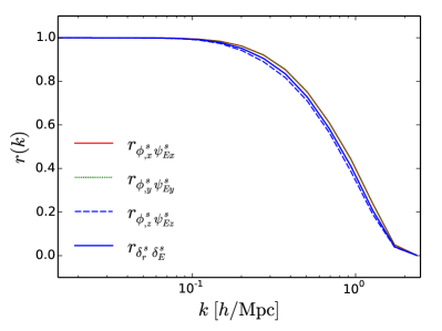
Figure 14: The cross-correlation coefficients of the reconstructed displacement components with the nonlinear displacement components (solid, dotted, dashed lines are for $x,y,z$-components respectively) and the reconstructed density field with the nonlinear displacement divergence.

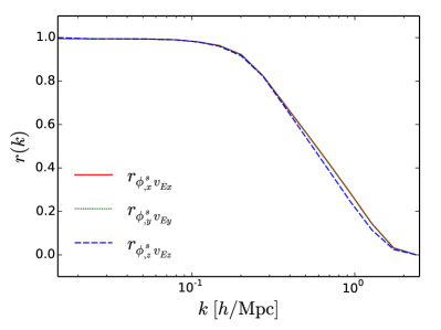
Figure 15: The cross-correlation coefficient of the reconstructed displacement with the Lagrangian velocity. The correlation for each component is larger than $0.5$ at $k\lesssim 0.43\ h/\mathrm{Mpc}$, much smaller than the scale where the nonlinear density field correlates with the linear density field.

In linear theory, the Lagrangian displacement only differs from the Lagrangian velocity by a factor $afH$. Their relation becomes complicated in higher order Lagrangian perturbation theory. Nevertheless, it is still interesting to study the cross correlation of the reconstructed displacement with the real Lagrangian velocity. Figure 15 shows the cross-correlation coefficients computed using the angular-averaged power spectra. The cross-correlation coefficient for each component is larger than $0.5$ at $k\lesssim 0.43\ h/\mathrm{Mpc}$, though the behavior of the $z$-direction is a little different from the other two directions. This scale is much smaller than the scale where the nonlinear density field correlates with the linear density field ($k\lesssim 0.17\ h/\mathrm{Mpc}$). Therefore, we expect that the new velocity reconstruction scheme based on the relation between the reconstructed displacement and the Lagrangian velocity would be better than the method based on the linearized continuity equation.

IV Applications

The prime application of nonlinear reconstruction is to reverse the large-scale bulk flows and improve the precision measurement of the BAO scale. The density field reconstructed with the dark matter density in real space has a comparable fidelity as the linear density field for measuring the BAO scale, since the BAO wiggles are washed out at $k>0.6\ h/\mathrm{Mpc}$ in both fields. The new reconstruction methods can restore the BAO signal of the linear density perfectly in the idealized situation Schmittfull et al. (2017); Wang et al. (2017). The shot noise limits the performance of reconstruction when we apply nonlinear reconstruction to real space halo fields Yu et al. (2017). The new reconstruction method requires a higher number density $\bar{n}\geq 10^{-3}\ (h/\mathrm{Mpc})^{3}$ to have a better performance than the standard reconstruction method Yu et al. (2017). In this paper we show that RSD further degrade the performance due to the nonlinearity of the shift velocity and the small-scale random velocity dispersion. Nevertheless, we still expect the new method to substantially improve the precision of the measured BAO scale of dense low redshift large-scale structure surveys, including SDSS main sample, DESI BGS, and 21 cm intensity mapping, while the improvement over standard reconstruction for less dense high redshift samples like BOSS LOWZ and CMASS will be moderate.

We have applied reconstruction to halo density fields in redshift space. The two-dimensional correlation coefficients of the reconstructed density field with the linear initial conditions are presented in Appendix D. To apply nonlinear reconstruction to observations, we need to consider several complicated effects. A practical issue related to this is the boundary of a survey region, which is not the periodic simulation box. This problem can be solved by embedding the observed galaxy density field into a uniform background. We have demonstrated a simple test about this solution in Appendix E. The practical application of nonlinear reconstruction to SDSS galaxy samples will be studied in a future paper.

The most innovative result of this paper is that the nonlinear reconstruction method can improve not only the BAO measurement but also the RSD measurement. The nonlinear mapping solved from the anisotropic redshift space density field includes the $E$-mode shift velocity $\bm{v}^{s}_{E}$, which contains cosmological information about the growth of structure. The reconstructed density field shares many similar features as the redshift space density field like the large-scale squashing effect and small-scale finger of God effect, but much more linear than the original redshift space density field. A large amount of shift nonlinearities has been removed in the nonlinear reconstruction. The number of linear modes that can be used to measure the growth rate is increased by about $30$–$40$ times after reconstruction. Therefore, we expect that this will significantly reduce uncertainties of the measured structure growth rate since the constraining power of galaxy surveys scales steeply with the number of modes included in the RSD analysis. In contrast to the BAO reconstruction, where nonlinear reconstruction still needs a higher number density to gain better performance than standard reconstruction, the RSD nonlinear reconstruction can always obtain better performance than without reconstruction, no matter the number density of galaxy samples. This has significant implications for constraining modified gravity theories using the measured linear structure growth rate. However, we still expect substantial improvements for the dense low-redshift surveys as discussed above while the performance for less dense samples will be limited by the shot noise.

The current BAO reconstruction involves displacing particles according to the large-scale linear displacement field computed from the observed galaxy density field with some certain model assumptions like the smoothing scale, galaxy bias, growth rate etc Eisenstein et al. (2007a). The results depend on the assumed fiducial model and have to be tested against different parameter choices, which are computationally expensive Padmanabhan et al. (2012). The new reconstruction method directly solves the displacement potential from the observed density field, which is a purely mathematical problem without any cosmological dynamics involved. The parameters like the halo bias and structure growth rate do affect the reconstructed density field, but they are to be jointly fitted when we model the power spectrum after reconstruction, while there are no cosmological parameters involved in the reconstruction process itself. This saves a large amount of computational costs when applying reconstruction to galaxy surveys to improve BAO and RSD measurements.

The fact that the reconstructed displacements correlate with the Lagrangian velocities to nonlinear scales in Lagrangian space implies that we can construct new peculiar velocity reconstruction schemes based on this relation. The current peculiar velocity reconstruction methods are often based on the linearized continuity equation like the one used to measure the kinematic Sunyaev-Zeldovich effect through cross correlation Schaan et al. (2016). The linearized continuity equation is

$$\dot{\delta}+\nabla\cdot\bm{v}=0.$$ (30)

Assuming the velocity is curl free, the velocity can be inferred from the density through

$$\bm{v}(\bm{k})=afH\frac{i\bm{k}}{k^{2}}\delta(\bm{k})W_{R}(k),$$ (31)

where $W_{R}(k)$ is a smoothing function with the characteristic scale $R$. The smoothing scale should be chosen close to the scale where linear theory breaks down Schmittfull et al. (2015); Seo et al. (2016). To make the above linear approximation valid, the nonlinear density field usually needs to be smoothed on scales $\sim 10\ \mathrm{Mpc}/h$ to remove small-scale nonlinearities. This is because all quantities defined in Eulerian space like $\delta(\bm{x})$ and $\bm{v}(\bm{x})$ involve very strong shift nonlinearities, which have to be reduced in order to apply the linear relation. However, a lot of cosmological information about small-scale velocities is lost in this process. The quantities defined in Lagrangian space like Lagrangian displacement $\bm{\psi}(\bm{q})$ and Lagrangian velocity $\bm{v}(\bm{q})$ are free of any nonlinear shift terms Baldauf et al. (2016a). This motivates us to develop new velocity reconstruction methods using the relation between Lagrangian quantities instead of Eulerian quantities.

In the Lagrangian perturbation theory, the Lagrangian displacement is solved as

$$\bm{\psi}(\bm{q},t)=\bm{\psi}^{(1)}(\bm{q},t)+\bm{\psi}^{(2)}(\bm{q},t)+\bm{\psi}^{(3)}(\bm{q},t)+\cdots,$$ (32)

where $\bm{\psi}^{(n)}\propto(\bm{\psi}^{(1)})^{n}$ is the $n$th-order solution. The Lagrangian velocity of mass element with initial coordinate $\bm{q}$ is the time derivative of the Lagrangian displacement

$$\bm{v}(\bm{q},t)=a\dot{\bm{x}}(\bm{q},t)=a\dot{\bm{\psi}}(\bm{q},t).$$ (33)

The time dependence of the $n$th-order solution $\bm{\psi}^{(n)}$ can be well approximated as $\bm{\psi}^{(n)}\propto D^{n}$. Therefore, the Lagrangian velocity can be expressed as

$$\bm{v}(\bm{q},t)=afH\bm{\psi}^{(1)}(\bm{q},t)+2afH\bm{\psi}^{(2)}(\bm{q},t)+\cdots.$$ (34)

The most direct and simple idea is to filter the reconstructed displacement field with the linear transfer function to minimize the difference with the linear displacement field. Then compute the Lagrangian velocity using the linear relation $\bm{v}^{(1)}(\bm{q})=afH\bm{\psi}^{(1)}(\bm{q})$ and next generate the Eulerian space velocity field using a velocity assignment method Zhang et al. (2015); Zheng et al. (2015). This $\mathcal{O}(1)$ velocity reconstruction is the Lagrangian space version of the current velocity reconstruction in Eulerian space. However, since much fewer shift nonlinearities are involved in Lagrangian space and the displacement and velocity correlate to a much smaller scale in Lagrangian space than the density and velocity in Eulerian space, we expect that the new method will have a better performance than the previous methods operated in Eulerian space. We can also compute the second-order solution $2afH\bm{\psi}^{(2)}$ using the linear transfer function filtered displacement since the displacement is much more linear than the Lagrangian velocity. Then we can use the second-order transfer functions to optimally combine $afH\bm{\psi}^{(1)}$ and $2afH\bm{\psi}^{(2)}$ to obtain the reconstructed Lagrangian velocity Schmittfull et al. (2017). The $\mathcal{O}(2)$ velocity reconstruction scheme is expected to better recover small-scale velocities. One more possibility is to directly correlate the reconstructed displacement with the nonlinear Lagrangian velocity and solve the optimal transfer function. The detailed tests of the new velocity reconstruction schemes and comparisons against the current velocity reconstruction method will be investigated in a future paper.

V Conclusions

In this paper we apply nonlinear reconstruction to redshift space nonlinear dark matter density field and reconstruct the displacement potential that describes the mapping from initial Lagrangian coordinates to final redshift space coordinates. We undo the shifts from Lagrangian positions to redshift space positions by mapping the nonlinear density field into a uniform field and reduce the associated nonlinearities significantly. The reconstructed density field is defined as the negative divergence of the reconstructed displacement or the negative Laplacian of the displacement potential. The cross-correlation coefficient between the reconstructed density field and the linear initial conditions is larger than $0.5$ at $k\lesssim 0.6h/\mathrm{Mpc}$ and $0.8$ at $k\lesssim 0.3\ h/\mathrm{Mpc}$. We note that the reconstructed density field shares similar properties with the redshift space nonlinear density field, including the nonlinear finger of God effect and linear Kaiser effect. However, the reconstructed density field involves much fewer nonlinearities related with the shifts from Lagrangian positions to redshift space positions. Therefore we expect this nonlinear reconstruction approach to substantially improve the cosmological information content of BAO and RSD for dense large-scale structure surveys.

Reconstruction of the nonlinear displacement field is not perfect and limited by several factors, including shell crossing, vorticity and grid limiters. The reconstruction is not sensitive to the parameters used for grid limiters like the maximal compression factor and expansion volume limit (see tests presented in Ref. Zhu et al. (2017)). The performance is mostly limited by shell crossing and vorticity. Note that the $B$-mode displacement will also change the mass distribution in the Universe in addition to the $E$-mode displacement. However, due to the limited degree of freedom, we can only reconstruct a scalar field (displacement potential) from the observed density field which is caused by both $E$- and $B$-mode displacements; as a result, this induces errors in the reconstructed displacement field. The mapping from Lagrangian coordinates to redshift space coordinates is not unique once shell crossing occurs. We can still define a coordinate system which we refer to as potential isobaric gauge/coordinates where the mass per volume element is approximately constant. However, the reconstructed displacement is not accurate in the regime where shell crossing occurs. The shell crossing induces a similar effect like the vorticity; they both cause changes in the mass distribution in the Universe, but we treat the observed density field as a field not affected by them. To disentangle these two effects, we need to consider reconstruction in the one-dimensional case, where the displacement field has no $B$-mode component. By performing reconstruction in the one-dimensional Universe, we can estimate the effect solely induced by shell crossing Zhu et al. (2016).

In addition to the effects discussed above, the correlation of the reconstructed density with the linear initial conditions is also affected by the inherent nonlinearities of the Lagrangian displacement and velocity. Although Lagrangian quantities like the displacement and velocity are free of shift terms, they are still affected by structure formation, which induces inherent nonlinearities Tassev and Zaldarriaga (2012b). These inherent nonlinearities cannot be removed by nonlinear reconstruction. In summary, the performance of initial condition reconstruction is limited by residual shift nonlinearities due to imperfect reconstruction of the nonlinear displacement field and nonlinearities of the displacement and velocity fields.

The nonlinear reconstruction approach provides a new route to measure the RSD effect. Instead of modeling the complicated mapping from real to redshift space, we can reconstruct the Lagrangian displacement and velocity directly and use the reconstructed density field to measure the anisotropic effects due to the peculiar velocity. When trying to model RSD, we are creating nonlinear effects to make the theoretical power spectrum look like the nonlinear power spectrum. This still does not improve the information in the power spectrum of the observed density field from surveys. However, reconstruction can reduce nonlinearities and reverse the mapping from Lagrangian coordinates to redshift space coordinates. The density field after reconstruction can be described using linear theory on scales where the redshift space density field already needs to be modeled using higher order perturbation theory.

The correlation of the reconstructed displacement with the Lagrangian velocity is much better than the correlation between density and velocity in Eulerian space. This implies that the new peculiar velocity reconstruction scheme can be constructed based on the relation between Lagrangian displacement and velocity. Since much fewer nonlinearities are involved in the new reconstruction schemes, we expect that the performance will be better than the Eulerian velocity reconstruction method. We propose several velocity reconstruction methods here and detailed tests will be presented in future.

In this paper we show that the nonlinear reconstruction not only works in real space but also can be implemented in redshift space. In addition to improving the linear BAO signals, we find that this nonlinear approach can also improve the RSD measurements since the reconstructed density field shares similar features as the redshift space nonlinear density field and much more linear modes are recovered after reconstruction. This could substantially recover cosmological information about BAO and RSD for dense low-redshift large structure surveys such as SDSS MGS, DESI BGS and 21 cm intensity mapping surveys.

Appendix A Lagrangian displacement field

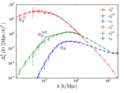
Figure 16: The power spectra for the decomposed Lagrangian displacements. The large-scale nonlinear displacement field is well described by the Zeldovich approximation for $k\lesssim 1\ h/\mathrm{Mpc}$. The nonlinear $E$-mode displacement becomes important at $k\gtrsim 1\ h/\mathrm{Mpc}$. The $B$-mode displacement only matters on very small scales for $k\gtrsim 10\ h/\mathrm{Mpc}$. The power spectra are computed using two sets of simulations with different resolutions.

Any vector field can be separated into a gradient part and a curl part. Hence we can decompose the real space nonlinear displacement as

$$\bm{\psi}(\bm{q})=\bm{\psi}_{E}(\bm{q})+\bm{\psi}_{B}(\bm{q}),$$ (35)

where $\bm{\psi}_{E}=(\bm{k}\cdot\bm{\psi})\bm{k}/k^{2}$ and $\bm{\psi}_{B}=\bm{\psi}-\bm{\psi}_{E}$. The $E$-mode displacement can be completely described by its divergence $\delta_{E}=-\nabla\cdot\bm{\psi}_{E}$. To see how the $E$-mode displacement correlates with the initial linear displacement, we carry out a further decomposition,

$$\bm{\psi}_{E}(\bm{q})=\bm{\psi}_{E}^{(l)}(\bm{q})+\bm{\psi}_{E}^{(nl)}(\bm{q}),$$ (36)

where

$$\bm{\psi}_{E}^{(l)}(\bm{k})=W(k)\bm{\psi}_{L}(\bm{k}),$$ (37)

and $W(k)={P_{\delta_{E}\delta_{L}}(k)}/{P_{\delta_{L}}(k)}$. Here, the superscript “$l$” denotes the part completely correlated with the linear displacement and “$nl$” denotes the part generated in nonlinear evolution. Then the nonlinear displacement is composed of three components

$$\bm{\psi}(\bm{q})=\bm{\psi}^{(l)}_{E}(\bm{q})+\bm{\psi}^{(nl)}_{E}(\bm{q})+\bm{\psi}_{B}(\bm{q}).$$ (38)

To measure the power spectra of these three components, we use two sets of simulations. The large box simulation involves $1024^{3}$ dark matter particles in a cubic box of length $600\ h/\mathrm{Mpc}$ and the small box simulation involves $1024^{3}$ dark matter particles in a cubic box of length $150\ h/\mathrm{Mpc}$. Each set of simulations has ten independent realizations with independent random initial conditions. The power spectrum of displacement is defined as

$$P_{\psi}(k)=\sum_{i}P_{\psi_{i}}(k),$$ (39)

where $i$ denotes $x$, $y$, or $z$ components. Figure 16 shows the power spectra measured from the two sets of simulations. The displacement power spectra are averaged over ten realizations. The nonlinear displacement field on large scales is well described by the Zeldovich displacement for $k\lesssim 1\ h/\mathrm{Mpc}$. The nonlinear $E$-mode displacement dominates over the linear $E$-mode displacement at $k=1\ h/\mathrm{Mpc}$. The $B$-mode displacement is negligible on scales larger than $k=10\ h/\mathrm{Mpc}$.

Appendix B Lagrangian velocity field

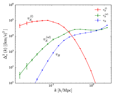
Figure 17: The power spectra for the decomposed Lagrangian velocity. The linear part of the velocity is dominant at $k\lesssim 0.25\ h/\mathrm{Mpc}$. The nonlinear contribution becomes important at $k=0.25\ h/\mathrm{Mpc}$. The curl part is already non-negligible on scales where the displacement can still described by the gradient.

The Lagrangian velocity describes the growth of the Lagrangian displacement,

$$\bm{v}(\bm{q})=\dot{\bm{\psi}}(\bm{q}),$$ (40)

where the dot denotes partial derivative with respect to time. Since both fields are defined in Lagrangian space, we can decompose the Lagrangian velocity similarly,

$$\bm{v}(\bm{q})=\bm{v}_{E}(\bm{q})+\bm{v}_{B}(\bm{q}),$$ (41)

where $\bm{v}_{E}=(\bm{k}\cdot\bm{v})\bm{k}/k^{2}$ and $\bm{v}_{B}=\bm{v}-\bm{v}_{E}$. The $E$-mode displacement can be decomposed into

$$\bm{v}_{E}(\bm{q})=\bm{v}_{E}^{(l)}(\bm{q})+\bm{v}_{E}^{(nl)}(\bm{q})$$ (42)

where

$$\bm{v}_{E}^{(l)}(\bm{k})=W_{v}(k)\bm{v}_{L}(\bm{k}).$$ (43)

Here, $\bm{v}_{L}(\bm{k})$ is derived from the linear density field,

$$\bm{v}_{L}(\bm{k})=afH\frac{i\bm{k}\delta_{L}(\bm{k})}{k^{2}},$$ (44)

and the velocity window function is

$$W_{v}(\bm{k})=\frac{P_{\theta_{E}\delta_{L}}(k)}{P_{\delta_{L}}(k)},$$ (45)

where $\theta_{E}=-\nabla\cdot\bm{v}/(afH)$. Now we can write the Lagrangian velocity as

$$\bm{v}(\bm{q})=\bm{v}_{E}^{(l)}(\bm{q})+\bm{v}_{E}^{(nl)}(\bm{q})+\bm{v}_{B}(\bm{q}),$$ (46)

where different velocities describe the growth of the corresponding Lagrangian displacements. The velocity power spectrum is defined as

$$P_{v}(k)=\sum_{i}P_{v_{i}}(k),$$ (47)

In Fig. 17, we show the velocity power spectra for different velocities. We only present the results from the large box simulations mentioned above since the Lagrangian velocity is much more nonlinear than the displacement. The linear theory can only describe the Lagrangian velocity up to $k\lesssim 0.25\ h/\mathrm{Mpc}$. The nonlinearities dominate on scales where the displacement can still be described by linear theory. The $B$-mode Lagrangian velocity is already non-negligible on scales $k\gtrsim 1.4\ h/\mathrm{Mpc}$. This is simply because the Lagrangian velocity corresponds to the most nonlinear contribution to the Lagrangian displacement as we discussed above.

The fact that the Lagrangian velocity is more nonlinear than the displacement implies that it is more important to study the nonlinearity of the velocity rather than the displacement to model the reconstructed density field. This also implies that we can use the much more linear displacement to calculate the higher order terms of the velocity field using perturbation theories, in order to construct $\mathcal{O}(2)$ peculiar velocity reconstruction schemes.

Appendix C Shift velocity field

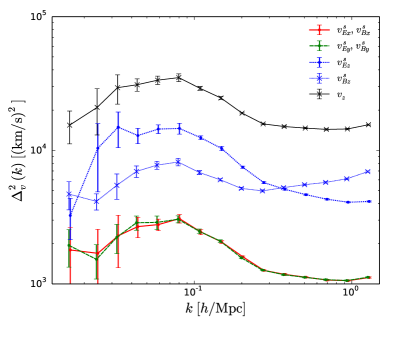
Figure 18: The power spectra for the different shift velocity components. The power spectrum of ${v^{s}_{Bz}}$ matches the linear theory prediction at $k\lesssim 0.1\ h/\mathrm{Mpc}$, while the other power spectra can be well described by linear perturbation theory at $k\lesssim 0.15\ h/\mathrm{Mpc}$. The power of $v^{s}_{Bz}$ becomes larger on smaller scales and dominates over $v^{s}_{Ez}$ at $k=0.36\ h/\mathrm{Mpc}$.

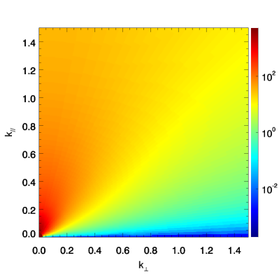
Figure 19: The two-dimensional power spectrum of the shift velocity divergence. Most power is concentrated in the $\mu$ bins close to $\mu\sim 1$ as expected. The values of the power spectrum are shown in the logarithmic scale.

The shift velocity corresponds to the $z$-component of the Lagrangian velocity,

$$\bm{v}^{s}(\bm{q})=v_{z}(\bm{q})\hat{z},$$ (48)

which describes the shift of a particle from the real space position to the redshift space position. We can write the shift velocity as

$$\bm{v}^{s}(\bm{q})=\bm{v}_{E}^{s}(\bm{q})+\bm{v}^{s}_{B}(\bm{q}),$$ (49)

where

$$\bm{v}^{s}_{E}(\bm{k})=\bigg{(}\frac{k_{x}k_{z}v_{z}(\bm{k})}{k^{2}},\frac{k_{y}k_{z}v_{z}(\bm{k})}{k^{2}},\frac{k_{z}k_{z}v_{z}(\bm{k})}{k^{2}}\bigg{)},$$ (50)

and

$$\bm{v}^{s}_{B}(\bm{k})=\bigg{(}-\frac{k_{x}k_{z}v_{z}(\bm{k})}{k^{2}},-\frac{k_{y}k_{z}v_{z}(\bm{k})}{k^{2}},\frac{(k^{2}-k_{z}^{2})v_{z}(\bm{k})}{k^{2}}\bigg{)}.$$

In linear theory, we can compute the power spectra of these velocities from the linear initial density. From the linear continuity equation, we have

$$v_{z}(\bm{k})=\frac{ik_{z}}{k^{2}}afH\delta_{L}(\bm{k}).$$ (52)

Then the angular averaged power spectrum of $v_{z}(\bm{k})$ is

$$P_{v_{z}}(k)=\frac{1}{3}(afH)^{2}P_{\delta_{L}}(k)/{k^{2}}.$$ (53)

In linear theory, the power spectra of different velocity components are

$$P_{v^{s}_{Ex}}(k)=P_{v^{s}_{Ey}}(k)=\frac{3}{35}P_{v_{z}}(k),$$ (54)

$$P_{v^{s}_{Ez}}(k)=\frac{15}{35}P_{v_{z}}(k),$$ (55)

$$P_{v^{s}_{Bx}}(k)=P_{v^{s}_{By}}(k)=\frac{3}{35}P_{v_{z}}(k),$$ (56)

and

$$P_{v^{s}_{Bz}}(k)=\frac{8}{35}P_{v_{z}}(k).$$ (57)

Figure 18 shows the velocity power spectra measured from the large box simulations. The effects of the $x$- and $y$-components of the $E$- and $B$-mode shift velocities are much smaller than the $z$-components. The power spectrum of ${v^{s}_{Bz}}$ matches the linear theory prediction at $k\lesssim 0.1\ h/\mathrm{Mpc}$, while the other power spectra can be well described by linear theory at $k\lesssim 0.15\ h/\mathrm{Mpc}$. The power of $v^{s}_{Bz}$ becomes larger on smaller scales and dominates over $v^{s}_{Ez}$ at $k=0.36\ h/\mathrm{Mpc}$. This behavior is not predicted within the linear perturbation theory. The strong nonlinearities in the shift velocity field cause the large power of $P_{v^{s}_{Bz}}(k)$ on small scales. This implies that the random velocity dispersion is large on small scales, which leads to the so-called finger of God effect.

Figure 19 shows the two-dimensional power spectrum of the negative divergence of the shift velocity $-\nabla\cdot\bm{v}^{s}$. We plot the power spectrum in logarithmic scale for visualization purposes. Most power of $-\nabla\cdot\bm{v}^{s}$ is concentrated in the $\mu$ bins close to $\mu\sim 1$ as expected. This causes part of the degradation of reconstruction performance along the line of sight direction.

Appendix D Reconstruction with halos

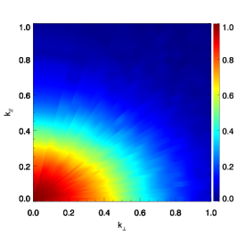
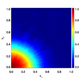
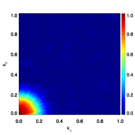
Figure 20: The two-dimensional cross-correlation coefficients of the halo reconstructed field with the linear field $(b_{1}+f\mu^{2})\delta_{L}(\bm{k})$ for $\bar{n}=2.77\times 10^{-2}$, $2.77\times 10^{-3}$, $2.77\times 10^{-4}\ (h/\mathrm{Mpc})^{3}$ (from left to right), respectively.

The dark matter field is nearly constant in Lagrangian space, while the halo field is not uniform in Lagrangian space. However, when we apply reconstruction, we still map the halo density field into a nearly uniform distribution as

$$\rho_{h}(\bm{x})d^{3}x=\rho(\bm{q})d^{3}q,$$ (58)

where $\rho_{h}(\bm{x})$ is the halo density field in Eulerian space. As a result, the reconstructed displacement is biased,

$$\bm{\psi}_{h}(\bm{k})=b(k)\bm{\psi}(\bm{k}),$$ (59)

where $b(k)$ is the bias factor of the displacement reconstructed from the halo field. At linear order the displacement bias is equal to the constant Eulerian halo bias,

$$\delta_{h}(\bm{x})=b_{1}\delta(\bm{x}),$$ (60)

where $b_{1}$ is the linear halo bias. However, the mapping from real to redshift space for the halo density field is still defined as the dark matter field

$$\rho_{h}(\bm{s})d^{3}s=\rho_{h}(\bm{x})d^{3}x,$$ (61)

where $\rho_{h}(\bm{s})$ is the redshift space halo density field. Thus the displacement reconstructed from halos in redshift space is

$$\bm{\psi}^{s}_{h}(\bm{k})=b(k)\bm{\psi}(\bm{k})+{\bm{v}^{s}(\bm{k})}/{aH}.$$ (62)

To quantify the performance of reconstruction with halos in redshift space, we should correlate the reconstructed field with $(b_{1}+f\mu^{2})\delta_{L}(\bm{k})$ instead of $(1+f\mu^{2})\delta_{L}(\bm{k})$.

Figure 20 shows the two-dimensional cross-correlation coefficients of the halo reconstructed density field with the linear field $(b_{1}+f\mu^{2})\delta_{L}(\bm{k})$. Three halo samples with number densities of $2.77\times 10^{-2}$, $2.77\times 10^{-3}$, and $2.77\times 10^{-4}\ (h/\mathrm{Mpc})^{3}$ are used for reconstruction. The bias factors are $b_{1}=0.68$, $0.92$, and $1.44$, respectively. We find that the correlation coefficients have the same anisotropic features as the result obtained with the dark matter density field, but the performance degrades with the lower number density. And also the less dense sample suffers less from the RSD effect.

Appendix E Reconstruction with survey mask

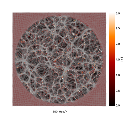
Figure 21: A slice of the density field from the high-resolution simulation. The curvilinear grid shows the Eulerian coordinate of each grid point of the potential isobaric coordinate. The reconstruction works very well within the spherical region though near the spherical boundary there are some artificial features caused by the discontinuities.

To apply nonlinear reconstruction to real observation data, we need to consider the boundary of a survey volume. In this appendix we present a simple test of reconstruction without the periodic boundary conditions. We take a spherical region with radius $140.625\ \mathrm{Mpc}/h$ from the high-precision simulation and set the density fluctuations $\rho(\bm{x})/\bar{\rho}$ in the outer space to 1. Then we perform reconstruction with this density field. Figure 21 shows a slice through the density field. We also plot the Eulerian positions of a uniform grid of potential isobaric coordinates on the density field slice. The reconstruction works very well within the spherical region though near the spherical boundary there are some artificial features caused by the discontinuities. However, this causes little degradation of reconstruction as the measure of a two-dimensional boundary is nearly $0$ in the three-dimensional space.

References

- Alam et al. (2017) S. Alam, M. Ata, S. Bailey, F. Beutler, D. Bizyaev, J. A. Blazek, A. S. Bolton, J. R. Brownstein, A. Burden, C.-H. Chuang, et al., MNRAS 470, 2617 (2017), eprint 1607.03155.
- Beutler et al. (2017a) F. Beutler, H.-J. Seo, A. J. Ross, P. McDonald, S. Saito, A. S. Bolton, J. R. Brownstein, C.-H. Chuang, A. J. Cuesta, D. J. Eisenstein, et al., MNRAS 464, 3409 (2017a), eprint 1607.03149.
- Ross et al. (2017) A. J. Ross, F. Beutler, C.-H. Chuang, M. Pellejero-Ibanez, H.-J. Seo, M. Vargas-Magaña, A. J. Cuesta, W. J. Percival, A. Burden, A. G. Sánchez, et al., MNRAS 464, 1168 (2017), eprint 1607.03145.
- Vargas-Magaña et al. (2016) M. Vargas-Magaña, S. Ho, A. J. Cuesta, R. O’Connell, A. J. Ross, D. J. Eisenstein, W. J. Percival, J. N. Grieb, A. G. Sánchez, J. L. Tinker, et al., ArXiv e-prints (2016), eprint 1610.03506.
- Beutler et al. (2017b) F. Beutler, H.-J. Seo, S. Saito, C.-H. Chuang, A. J. Cuesta, D. J. Eisenstein, H. Gil-Marín, J. N. Grieb, N. Hand, F.-S. Kitaura, et al., MNRAS 466, 2242 (2017b), eprint 1607.03150.
- Grieb et al. (2017) J. N. Grieb, A. G. Sánchez, S. Salazar-Albornoz, R. Scoccimarro, M. Crocce, C. Dalla Vecchia, F. Montesano, H. Gil-Marín, A. J. Ross, F. Beutler, et al., MNRAS 467, 2085 (2017), eprint 1607.03143.
- Sánchez et al. (2017) A. G. Sánchez, J. N. Grieb, S. Salazar-Albornoz, S. Alam, F. Beutler, A. J. Ross, J. R. Brownstein, C.-H. Chuang, A. J. Cuesta, D. J. Eisenstein, et al., MNRAS 464, 1493 (2017), eprint 1607.03146.
- Satpathy et al. (2017) S. Satpathy, S. Alam, S. Ho, M. White, N. A. Bahcall, F. Beutler, J. R. Brownstein, C.-H. Chuang, D. J. Eisenstein, J. N. Grieb, et al., MNRAS 469, 1369 (2017), eprint 1607.03148.
- Zhao et al. (2017) G.-B. Zhao, Y. Wang, S. Saito, D. Wang, A. J. Ross, F. Beutler, J. N. Grieb, C.-H. Chuang, F.-S. Kitaura, S. Rodriguez-Torres, et al., MNRAS 466, 762 (2017), eprint 1607.03153.
- Bandura et al. (2014) K. Bandura, G. E. Addison, M. Amiri, J. R. Bond, D. Campbell-Wilson, L. Connor, J.-F. Cliche, G. Davis, M. Deng, N. Denman, et al., in Ground-based and Airborne Telescopes V (2014), vol. 9145 of Proc. SPIE, p. 914522, eprint 1406.2288.
- Xu et al. (2015) Y. Xu, X. Wang, and X. Chen, ApJ 798, 40 (2015), eprint 1410.7794.
- DESI Collaboration et al. (2016) DESI Collaboration, A. Aghamousa, J. Aguilar, S. Ahlen, S. Alam, L. E. Allen, C. Allende Prieto, J. Annis, S. Bailey, C. Balland, et al., ArXiv e-prints (2016), eprint 1611.00036.
- Takada et al. (2014) M. Takada, R. S. Ellis, M. Chiba, J. E. Greene, H. Aihara, N. Arimoto, K. Bundy, J. Cohen, O. Doré, G. Graves, et al., PASJ 66, R1 (2014).
- Eisenstein et al. (2007a) D. J. Eisenstein, H.-J. Seo, E. Sirko, and D. N. Spergel, ApJ 664, 675 (2007a), eprint astro-ph/0604362.
- Tassev and Zaldarriaga (2012a) S. Tassev and M. Zaldarriaga, J. Cosmology Astropart. Phys 10, 006 (2012a), eprint 1203.6066.
- Schmittfull et al. (2015) M. Schmittfull, Y. Feng, F. Beutler, B. Sherwin, and M. Y. Chu, Phys. Rev. D 92, 123522 (2015), eprint 1508.06972.
- Obuljen et al. (2017) A. Obuljen, F. Villaescusa-Navarro, E. Castorina, and M. Viel, J. Cosmology Astropart. Phys 9, 012 (2017), eprint 1610.05768.
- Padmanabhan et al. (2012) N. Padmanabhan, X. Xu, D. J. Eisenstein, R. Scalzo, A. J. Cuesta, K. T. Mehta, and E. Kazin, MNRAS 427, 2132 (2012), eprint 1202.0090.
- Anderson et al. (2012) L. Anderson, E. Aubourg, S. Bailey, D. Bizyaev, M. Blanton, A. S. Bolton, J. Brinkmann, J. R. Brownstein, A. Burden, A. J. Cuesta, et al., MNRAS 427, 3435 (2012), eprint 1203.6594.
- Kazin et al. (2014) E. A. Kazin, J. Koda, C. Blake, N. Padmanabhan, S. Brough, M. Colless, C. Contreras, W. Couch, S. Croom, D. J. Croton, et al., MNRAS 441, 3524 (2014), eprint 1401.0358.
- Anderson et al. (2014) L. Anderson, É. Aubourg, S. Bailey, F. Beutler, V. Bhardwaj, M. Blanton, A. S. Bolton, J. Brinkmann, J. R. Brownstein, A. Burden, et al., MNRAS 441, 24 (2014), eprint 1312.4877.
- Tojeiro et al. (2014) R. Tojeiro, A. J. Ross, A. Burden, L. Samushia, M. Manera, W. J. Percival, F. Beutler, J. Brinkmann, J. R. Brownstein, A. J. Cuesta, et al., MNRAS 440, 2222 (2014), eprint 1401.1768.
- Ross et al. (2015) A. J. Ross, L. Samushia, C. Howlett, W. J. Percival, A. Burden, and M. Manera, MNRAS 449, 835 (2015), eprint 1409.3242.
- Eisenstein et al. (2007b) D. J. Eisenstein, H.-J. Seo, and M. White, ApJ 664, 660 (2007b), eprint astro-ph/0604361.
- Padmanabhan et al. (2009) N. Padmanabhan, M. White, and J. D. Cohn, Phys. Rev. D 79, 063523 (2009), eprint 0812.2905.
- Noh et al. (2009) Y. Noh, M. White, and N. Padmanabhan, Phys. Rev. D 80, 123501 (2009), eprint 0909.1802.
- Tassev and Zaldarriaga (2012b) S. Tassev and M. Zaldarriaga, J. Cosmology Astropart. Phys 4, 013 (2012b), eprint 1109.4939.
- Tassev (2014) S. Tassev, J. Cosmology Astropart. Phys 6, 008 (2014), eprint 1311.4884.
- Seo et al. (2016) H.-J. Seo, F. Beutler, A. J. Ross, and S. Saito, MNRAS 460, 2453 (2016), eprint 1511.00663.
- Zhu et al. (2017) H.-M. Zhu, Y. Yu, U.-L. Pen, X. Chen, and H.-R. Yu, Phys. Rev. D 96, 123502 (2017), eprint 1611.09638.
- Schmittfull et al. (2017) M. Schmittfull, T. Baldauf, and M. Zaldarriaga, Phys. Rev. D 96, 023505 (2017), eprint 1704.06634.
- Shi et al. (2018) Y. Shi, M. Cautun, and B. Li, Phys. Rev. D 97, 023505 (2018), eprint 1709.06350.
- Seljak et al. (2017) U. Seljak, G. Aslanyan, Y. Feng, and C. Modi, J. Cosmology Astropart. Phys 12, 009 (2017), eprint 1706.06645.
- Jackson (1972) J. C. Jackson, MNRAS 156, 1P (1972), eprint 0810.3908.
- Sargent and Turner (1977) W. L. W. Sargent and E. L. Turner, ApJ 212, L3 (1977).
- Peebles (1980) P. J. E. Peebles, The large-scale structure of the universe (1980).
- Kaiser (1987) N. Kaiser, MNRAS 227, 1 (1987).
- Peacock and Dodds (1994) J. A. Peacock and S. J. Dodds, MNRAS 267, 1020 (1994), eprint astro-ph/9311057.
- Ballinger et al. (1996) W. E. Ballinger, J. A. Peacock, and A. F. Heavens, MNRAS 282, 877 (1996), eprint astro-ph/9605017.
- Fisher (1995) K. B. Fisher, ApJ 448, 494 (1995).
- Heavens et al. (1998) A. F. Heavens, S. Matarrese, and L. Verde, MNRAS 301, 797 (1998), eprint astro-ph/9808016.
- White (2001) M. White, MNRAS 321, 1 (2001), eprint astro-ph/0005085.
- Seljak (2001) U. Seljak, MNRAS 325, 1359 (2001), eprint astro-ph/0009016.
- Kang et al. (2002) X. Kang, Y. P. Jing, H. J. Mo, and G. Börner, MNRAS 336, 892 (2002), eprint astro-ph/0201124.
- Scoccimarro (2004) R. Scoccimarro, Phys. Rev. D 70, 083007 (2004), eprint astro-ph/0407214.
- Tinker et al. (2006) J. L. Tinker, D. H. Weinberg, and Z. Zheng, MNRAS 368, 85 (2006), eprint astro-ph/0501029.
- Tinker (2007) J. L. Tinker, MNRAS 374, 477 (2007), eprint astro-ph/0604217.
- Desjacques and Sheth (2010) V. Desjacques and R. K. Sheth, Phys. Rev. D 81, 023526 (2010), eprint 0909.4544.
- Taruya et al. (2010) A. Taruya, T. Nishimichi, and S. Saito, Phys. Rev. D 82, 063522 (2010), eprint 1006.0699.
- Matsubara (2011) T. Matsubara, Phys. Rev. D 83, 083518 (2011), eprint 1102.4619.
- Okumura and Jing (2011) T. Okumura and Y. P. Jing, ApJ 726, 5 (2011), eprint 1004.3548.
- Okamura et al. (2011) T. Okamura, A. Taruya, and T. Matsubara, J. Cosmology Astropart. Phys 8, 012 (2011), eprint 1105.1491.
- Sato and Matsubara (2011) M. Sato and T. Matsubara, Phys. Rev. D 84, 043501 (2011), eprint 1105.5007.
- Jennings et al. (2011) E. Jennings, C. M. Baugh, and S. Pascoli, MNRAS 410, 2081 (2011), eprint 1003.4282.
- Reid and White (2011) B. A. Reid and M. White, MNRAS 417, 1913 (2011), eprint 1105.4165.
- Seljak and McDonald (2011) U. Seljak and P. McDonald, J. Cosmology Astropart. Phys 11, 039 (2011), eprint 1109.1888.
- Okumura et al. (2012a) T. Okumura, U. Seljak, P. McDonald, and V. Desjacques, J. Cosmology Astropart. Phys 2, 010 (2012a), eprint 1109.1609.
- Okumura et al. (2012b) T. Okumura, U. Seljak, and V. Desjacques, J. Cosmology Astropart. Phys 11, 014 (2012b), eprint 1206.4070.
- Kwan et al. (2012) J. Kwan, G. F. Lewis, and E. V. Linder, ApJ 748, 78 (2012), eprint 1105.1194.
- Zhang et al. (2013) P. Zhang, J. Pan, and Y. Zheng, Phys. Rev. D 87, 063526 (2013), eprint 1207.2722.
- Zheng et al. (2013) Y. Zheng, P. Zhang, Y. Jing, W. Lin, and J. Pan, Phys. Rev. D 88, 103510 (2013), eprint 1308.0886.
- Ishikawa et al. (2014) T. Ishikawa, T. Totani, T. Nishimichi, R. Takahashi, N. Yoshida, and M. Tonegawa, MNRAS 443, 3359 (2014), eprint 1308.6087.
- White et al. (2015) M. White, B. Reid, C.-H. Chuang, J. L. Tinker, C. K. McBride, F. Prada, and L. Samushia, MNRAS 447, 234 (2015), eprint 1408.5435.
- Bianchi et al. (2015) D. Bianchi, M. Chiesa, and L. Guzzo, MNRAS 446, 75 (2015), eprint 1407.4753.
- Bianchi et al. (2016) D. Bianchi, W. J. Percival, and J. Bel, MNRAS 463, 3783 (2016), eprint 1602.02780.
- Jennings et al. (2016) E. Jennings, R. H. Wechsler, S. W. Skillman, and M. S. Warren, MNRAS 457, 1076 (2016), eprint 1508.01803.
- Hand et al. (2017) N. Hand, U. Seljak, F. Beutler, and Z. Vlah, J. Cosmology Astropart. Phys 10, 009 (2017), eprint 1706.02362.
- Matsubara (2008a) T. Matsubara, Phys. Rev. D 77, 063530 (2008a), eprint 0711.2521.
- Matsubara (2008b) T. Matsubara, Phys. Rev. D 78, 083519 (2008b), eprint 0807.1733.
- Matsubara (2014) T. Matsubara, Phys. Rev. D 90, 043537 (2014).
- Porto et al. (2014) R. A. Porto, L. Senatore, and M. Zaldarriaga, J. Cosmology Astropart. Phys 5, 022 (2014), eprint 1311.2168.
- Carlson et al. (2013) J. Carlson, B. Reid, and M. White, MNRAS 429, 1674 (2013), eprint 1209.0780.
- Vlah et al. (2015a) Z. Vlah, U. Seljak, and T. Baldauf, Phys. Rev. D 91, 023508 (2015a), eprint 1410.1617.
- Seljak and Vlah (2015) U. Seljak and Z. Vlah, Phys. Rev. D 91, 123516 (2015), eprint 1501.07512.
- Vlah et al. (2015b) Z. Vlah, M. White, and A. Aviles, J. Cosmology Astropart. Phys 9, 014 (2015b), eprint 1506.05264.
- Vlah et al. (2016) Z. Vlah, E. Castorina, and M. White, J. Cosmology Astropart. Phys 12, 007 (2016), eprint 1609.02908.
- McQuinn and White (2016) M. McQuinn and M. White, J. Cosmology Astropart. Phys 1, 043 (2016), eprint 1502.07389.
- Baldauf et al. (2016a) T. Baldauf, E. Schaan, and M. Zaldarriaga, J. Cosmology Astropart. Phys 3, 017 (2016a), eprint 1505.07098.
- Baldauf et al. (2016b) T. Baldauf, E. Schaan, and M. Zaldarriaga, J. Cosmology Astropart. Phys 3, 007 (2016b), eprint 1507.02255.
- Pen (1995) U.-L. Pen, ApJS 100, 269 (1995).
- Pen (1998) U.-L. Pen, ApJS 115, 19 (1998).
- Harnois-Déraps et al. (2013) J. Harnois-Déraps, U.-L. Pen, I. T. Iliev, H. Merz, J. D. Emberson, and V. Desjacques, MNRAS 436, 540 (2013), eprint 1208.5098.
- White (2015) M. White, MNRAS 450, 3822 (2015).
- Hikage et al. (2017) C. Hikage, K. Koyama, and A. Heavens, Phys. Rev. D 96, 043513 (2017), eprint 1703.07878.
- Wang et al. (2017) X. Wang, H.-R. Yu, H.-M. Zhu, Y. Yu, Q. Pan, and U.-L. Pen, ApJ 841, L29 (2017), eprint 1703.09742.
- Yu et al. (2017) Y. Yu, H.-M. Zhu, and U.-L. Pen, ApJ 847, 110 (2017), eprint 1703.08301.
- Schaan et al. (2016) E. Schaan, S. Ferraro, M. Vargas-Magaña, K. M. Smith, S. Ho, S. Aiola, N. Battaglia, J. R. Bond, F. De Bernardis, E. Calabrese, et al., Phys. Rev. D 93, 082002 (2016), eprint 1510.06442.
- Zhang et al. (2015) P. Zhang, Y. Zheng, and Y. Jing, Phys. Rev. D 91, 043522 (2015), eprint 1405.7125.
- Zheng et al. (2015) Y. Zheng, P. Zhang, and Y. Jing, Phys. Rev. D 91, 043523 (2015), eprint 1409.6809.
- Zhu et al. (2016) H.-M. Zhu, U.-L. Pen, and X. Chen, ArXiv e-prints (2016), eprint 1609.07041.