Long-Term Online Smoothing Prediction
Using Expert Advice

Alexander Korotin a.korotin@skoltech.ru Vladimir V’yugin v.vuygin@skoltech.ru Evgeny Burnaev e.burnaev@skoltech.ru Skolkovo Institute of Science and Technology
Abstract

For the prediction with experts’ advice setting we construct forecasting algorithms that suffer loss not much more than any expert in the pool. In contrast to the standard approach, we investigate the case of long-term forecasting of time series and consider two scenarios. In the first one, at each step $t$ the learner has to combine the point forecasts of the experts issued for the time interval $[t+1,t+d]$ ahead. Our approach implies that at each time step experts issue point forecasts for arbitrary many steps ahead and then the learner (algorithm) combines these forecasts and the forecasts made earlier into one vector forecast for steps $[t+1,t+d]$. By combining past and the current long-term forecasts we obtain a smoothing mechanism that protects our algorithm from temporary trend changes, noise and outliers. In the second scenario, at each step $t$ experts issue a prediction function, and the learner has to combine these functions into the single one, which will be used for long-term time-series prediction. For each scenario we develop an algorithm for combining experts forecasts and prove $O(\ln T)$ adversarial regret upper bound for both algorithms.

keywords:
long-term online smoothing forecasting , prediction with expert advice , online smoothing regression
††journal: Neurocomputing

1 Introduction

The problem of long-term forecasting of time series is of high practical importance. For example, nowadays nearly everybody uses long-term weather forecasts [1, 2] (24 hour, 7 days, etc.) provided by local weather forecasting platforms. Road traffic and jams forecasts [3, 4, 5] are being actively used in many modern navigating systems. Forecasts of energy consumption and costs [6], web traffic [7] and stock prices [8, 9] are also widely used in practice.

Many state-of-the-art (e.g. ARIMA [10]) and modern (e.g. Facebook Prophet111https://github.com/facebook/prophet [11]) time series forecasting approaches produce a model that is capable of predicting arbitrarily many steps ahead. The advantage of such models is that when building the final forecast at each step $t$ for interval ${[t+1,t+d]}$ ahead, one may use forecasts made earlier at the steps ${\tau<t}$. Forecasts of each step ${\tau<t}$ are made using less of the observed data. Nevertheless, they can be more robust to noise, outliers and novelty of the time interval ${[\tau+1,t]}$. Thus, the usage of such outdated forecasts may prove useful, especially if time series is stationary.

In general, we consider the game-theoretic on-line learning model in which a master (aggregating) algorithm has to combine predictions from a set of experts. The problem setting we investigate can be considered as the part of Decision-Theoretic Online Learning (DTOL) or Prediction with Expert Advice (PEA) framework (see e.g. [12, 13, 14, 15, 16, 17] among others). In this framework the learner is usually called the aggregating algorithm. The aggregating algorithm combines the predictions from a set of experts in the online mode during time steps $t=1,2,\dots,T$.

In practice for time series prediction the square loss function is widely used. The square loss function is mixable [15]. For mixable loss functions Vovk’s aggregating algorithm (AA) [15, 18] is the most appropriate, since it has theoretically best performance among all known algorithms. We use the aggregating algorithm as the base and modify it for the long-term forecasting.

The long-term forecasting considered in this paper is a case of the forecasting with a delayed feedback. As far as we know, the problem of the delayed feedback forecasting was first considered by [19].

In this paper we consider the two scenarios of the long-term forecasting. In the first one, at each step $t$ the learner has to combine the point forecasts of the experts issued for the time interval $[t+1,t+d]$ ahead. In the second scenario, at each step $t$ experts issue prediction functions, and the learner has to combine these functions into the single one, that will be used for long-term time-series prediction.

The first theoretical problem we investigate in the paper is the effective usage of the outdated forecasts. Formally, the learner is given $N$ basic forecasting models. Each model ${n=1,2,\dots,N}$ at every step $t$ produces infinite forecast for the steps ${t+1,t+2,\dots}$ ahead. The goal of the learner at each step $t$ is to combine the current models’ forecasts and the forecasts made earlier into one aggregated long-term forecast for the time interval $[t+1,t+d]$ ahead. We develop an algorithm to efficiently combine these forecasts.

Our main idea is to replicate any expert $n$ in an infinite sequence of auxiliary experts $(n,\tau)$, where $\tau=1,2,\dots$. Each expert $(n,\tau)$ issues at time moment $\tau$ an infinite sequence of forecasts for time moments $\tau+1,\tau+2,\dots$. Only a finite number of the experts are available at any time moment. The setting presented in this paper is valid also in case where only one expert ($N=1$) is given. At any time moment $t$ the AA uses predictions of each expert $(n,\tau)$ for the time interval $[t+1,t+d]$ (made by expert $n$ at time $\tau\leq t$). In our case, the performance of the AA on the step $t$ is measured by the regret $r_{t}$ which is the difference between the average loss of the aggregating algorithm suffered on time interval $[d+1,T]$ and the average loss of the best auxiliary expert $(n,\tau)$ suffered on the same time interval. Note that the recent related work is [20] where an algorithm with tight upper bound for predicting vector valued outcomes was presented.

In the second part of our paper we consider the online supervised learning scenario. The data is represented by pairs $(x,y)$ of predictor-response variables. Instead of point or interval predictions, the experts and the learner present predictions in the form of functions $F(x)$ from signals $x$. Signals $x_{t}$ appear gradually over time $t$ and allow to calculate forecasts as the values $F(x_{t})$ of these functions. For this problem we present method for smoothing regression using expert advice.

The article is structured as follows. In SectionΒ 2 we give some preliminary notions. In SectionΒ 3 we present the algorithm for combining long-term forecasts of the experts. TheoremΒ 1 presents a performance bound $O(\log(NT))$ for the regret of the corresponding algorithms.

In SectionΒ 4 we apply PEA approach for a case of the online supervised learning and develop an algorithm for online smoothing regression. Also, we provide experiments conducted on synthetic data and show the effectiveness of the proposed method. In A some auxiliary results are presented.

2 Preliminaries

In this section we recall the main ideas of prediction with expert advice theory. Let a pool of $N$ experts be given. Suppose that elements $y_{1},y_{2},\dots$ of a time series are revealed online – step by step. Learning proceeds in trials $t=1,\ldots,T$. At each time moment $t$ experts $i\in\{1,\dots,N\}$ present their predictions $c^{i}_{t}$ and the aggregating algorithm presents its own forecast $\gamma_{t}$. When the corresponding outcome(s) are revealed, all the experts suffer their losses using a loss function: $l^{i}_{t}=\lambda(y_{t},c^{i}_{t})$, $i=1,\dots,N$. Let $h_{t}=\lambda(y_{t},\gamma_{t})$ be the loss of the aggregating algorithm. The cumulative loss suffered by any expert $i$ and by AA during $T$ steps are defined as

$\displaystyle L_{T}^{i}=\sum\limits_{t=1}^{T}l_{t}^{i}\mbox{ and }H_{T}=\sum\limits_{t=1}^{T}h_{t}.$

The performance of the algorithm w.r.t. an expert $i$ can be measured by the regret $R^{i}_{T}=H_{T}-L^{i}_{T}$.

The goal of the aggregating algorithm is to minimize the regret with respect to each expert. In order to achieve this goal, at each time moment $t$, the aggregating algorithm evaluates performance of the experts in the form of a vector of experts’ weights ${\bf w}_{t}=(w_{1,t},\dots,w_{N,t})$, where $\|{\bf w}_{t}\|_{1}=1$ and $w_{i,t}\geq 0$ for all $i$. The weight $w_{i,t}$ of an expert $i$ is an estimate of the quality of the expert’s predictions at step $t$. In classical setting (see [13], [14] among others), the process of expert $i$ weights updating is based on the method of exponential weighting with a learning rate $\eta>0$:

$\displaystyle w^{\mu}_{i,t}=\frac{w_{i,t}e^{-\eta l_{t}^{i}}}{\sum\limits_{j=1}^{N}w_{j,t}e^{-\eta l_{t}^{j}}},$ (1)

where ${\bf w}_{1}$ is some weight vector, for example, ${{\bf w}_{1}=(\frac{1}{N},\dots,\frac{1}{N})}$. In classical setting, we prepare weights ${\bf w}_{t+1}={\bf w}^{\mu}_{t}$ for using at the next step or, in a more general case of the $d$-th outcome ahead prediction, we define ${{\bf w}_{t+d}={\bf w}^{\mu}_{t}}$, where $d\geq 1$.

The Vovk’s aggregating algorithm (AA) ([14], [15]) is the base algorithm in our study. Let us explain the main ideas of learning with AA.

We consider the learning with a mixable loss function $\lambda(y,\gamma)$. Here $y$ is an element of some set of outcomes $y$, and $\gamma$ is an element of some set of forecasts $\Gamma$. The experts $1\leq i\leq N$ present the forecasts $c_{i}\in\Gamma$.

In this case the main tool is a superprediction function

$\displaystyle g(y)=-\frac{1}{\eta}\ln\sum\limits_{i=1}^{N}e^{-\eta\lambda(y,c_{i})}p_{i},$

where ${\bf p}=(p_{1},\dots,p_{N})$ is a probability distribution on the set of all experts and ${\bf c}=(c_{1},\dots,c_{N})$ is a vector of the experts predictions.

The loss function $\lambda$ is mixable if for any probability distribution ${\bf p}$ on the set of experts and for any set of experts predictions ${\bf c}$ a value of $\gamma$ exists such that

$\displaystyle\lambda(y,\gamma)\leq g(y)$ (2)

for all $y$.

We fix some rule $\gamma={\rm Subst}({\bf c},{\bf p})$ for computing a forecast satisfying (2). ${\rm Subst}$ is called a substitution function.

It will be proved in Section A that using the rules (1) and (2) for defining weights and the forecasts in the online mode we obtain

$$H_{T}\leq\min_{1\leq i\leq N}L^{i}_{T}+\frac{\ln N}{\eta}$$

for all $T$.

A loss function $\lambda(y,\gamma)$ is $\eta$-exponential concave if for any $y$ the function $e^{-\eta\lambda(y,\gamma)}$ is concave w.r.t. $\gamma$. By definition any $\eta$-exponential concave function is $\eta$-mixable.

The square loss function $\lambda(y,\gamma)=(y-\gamma)^{2}$ is $\eta$-mixable for any $\eta$ such that $0<\eta\leq\frac{1}{2B^{2}}$, where $y$ and $\gamma$ are a real numbers and $y\in[-B,B]$ for some $B>0$, see [14, 15].

By [15] and [18], for the square loss function, the corresponding forecast can be defined as

$\displaystyle\gamma={\rm Subst}({\bf c},{\bf p})=\frac{1}{4B}(g(-B)-g(B))=\frac{1}{4\eta B}\ln\frac{\sum\limits_{i=1}^{N}p_{i}e^{-\eta(B-c_{i})^{2}}}{\sum\limits_{i=1}^{N}p_{i}e^{-\eta(B+c_{i})^{2}}}.$ (3)

For the $\eta$-exponential concave loss function we can also use a more straightforward expression for the substitution function:

$\displaystyle\gamma={\rm Subst}({\bf c},{\bf p})=\sum_{i=1}^{N}c_{i}p_{i}.$ (4)

The inequality (2) also holds for all $y$.

The square loss function is $\eta$-exponential concave for $0<\eta\leq\frac{1}{8B^{2}}$. However, the definition (4) results in four times more regret (see [21] and Section A).

3 Algorithm for Combining Long-term Forecasts of Experts.

In this section we consider an extended setting. At each time moment $t$ each expert $n\in\{1,\dots,N\}$ presents an infinite sequence ${\bf c}^{n}_{t}=(c^{n}_{t,1},c^{n}_{t,2},\dots)$ of forecasts for the time moments $t+1,t+2,t+3,\dots$. A sequence of the corresponding confidence levels ${\bf p}^{n}_{t}=(p^{n}_{t,1},p^{n}_{t,2},\dots)$ also can be presented at time moment $t$. Each element of this sequence is a number between 0 and 1. If $p^{n}_{t,i}<1$, then it means that we use the forecast $p^{n}_{t,i}$ only partially (e.g. it may become obsolete with time). If $p^{n}_{t,i}=0$ then the corresponding forecast is not taken into account at all.222For example, in applications, it is convenient for some $d$ to set $p^{n}_{t,i}=0$ for all $i>d$, since too far predictions become obsolete. Confidence levels can be set by the expert itself or by the learner.333 The setting of prediction with experts that report their confidences as a number in the interval $[0,1]$ was first studied by [22] and further developed by [23].

At each time moment $t$ we observe sequences ${\bf c}^{n}_{\tau}$, ${\bf p}^{n}_{\tau}$ issued by the experts $1\leq n\leq N$ at the time moments $\tau\leq t$. To aggregate the forecasts of all experts, we convert any β€œreal” expert $n$ into the infinite sequence of the auxiliary experts $(n,\tau)$, where $1\leq\tau<\infty$.

At each time moment $t$ expert $(n,\tau)$ presents his forecast which is the segment of the sequence ${\bf c}^{n}_{\tau}$ of length $d$ starting at its $(t-\tau+1)$th element. More precisely, the forecast of the auxiliary expert $(n,\tau)$ is a vector

$${\bf c}^{(n,\tau)}_{t}=(c^{(n,\tau)}_{t,1},\dots,c^{(n,\tau)}_{t,d}),$$

where for ${1\leq s\leq d}$ we set ct,s(n,Ο„)=cΟ„,tβˆ’Ο„+snsubscriptsuperscriptπ‘π‘›πœπ‘‘π‘ subscriptsuperscriptπ‘π‘›πœπ‘‘πœπ‘ c^{(n,\tau)}_{t,s}=c^{n}_{\tau,t-\tau+s}.

We also denote the corresponding segments of confidence levels by

$${{\bf p}^{(n,\tau)}_{t}=(p^{(n,\tau)}_{t,1},\dots,p^{(n,\tau)}_{t,d})},$$

where pt,s(n,Ο„)=pΟ„,tβˆ’Ο„+snsubscriptsuperscriptπ‘π‘›πœπ‘‘π‘ subscriptsuperscriptπ‘π‘›πœπ‘‘πœπ‘ p^{(n,\tau)}_{t,s}=p^{n}_{\tau,t-\tau+s} for $1\leq\tau\leq t$ and pt,s(n,Ο„)=0subscriptsuperscriptπ‘π‘›πœπ‘‘π‘ 0p^{(n,\tau)}_{t,s}=0 for $\tau>t$.

Using the losses suffered by the experts $(n,\tau)$ (for ${\tau\leq t}$) on the time interval $[t-d+1,t]$, the aggregating algorithm updates the weights $w_{(n,\tau),t}$ of all the experts $(n,\tau)$ by the rule (1). We denote these weights by $w_{(n,\tau),t+d}$ and use them for computing the aggregated interval forecast for $d$ time moments $t+1,\dots,t+d$ ahead

$$\gamma_{t}=(\gamma_{t,1},\dots,\gamma_{t,d}).$$

We use the fixed point method by [24]. Define the virtual forecasts of the experts $(n,\tau)$:

c~t,s(n,Ο„)={ct,s(n,Ο„)​ with probability ​pt,s(n,Ο„),Ξ³t,s​ with probability ​1βˆ’pt,s(n,Ο„).subscriptsuperscript~π‘π‘›πœπ‘‘π‘ casessubscriptsuperscriptπ‘π‘›πœπ‘‘π‘ Β with probabilityΒ subscriptsuperscriptπ‘π‘›πœπ‘‘π‘ subscript𝛾𝑑𝑠 with probabilityΒ 1subscriptsuperscriptπ‘π‘›πœπ‘‘π‘ \tilde{c}^{(n,\tau)}_{t,s}=\left\{\begin{array}[]{l}c^{(n,\tau)}_{t,s}\mbox{ with probability }p^{(n,\tau)}_{t,s},\\ \gamma_{t,s}\mbox{ with probability }1-p^{(n,\tau)}_{t,s}.\end{array}\right.

where $1\leq n\leq N$ and $1\leq\tau<\infty$.

We consider any confidence level pt,s(n,Ο„)subscriptsuperscriptπ‘π‘›πœπ‘‘π‘ p^{(n,\tau)}_{t,s} as a probability distribution 𝐩t,s(n,Ο„)=(pt,s(n,Ο„),1βˆ’pt,s(n,Ο„))subscriptsuperscriptπ©π‘›πœπ‘‘π‘ subscriptsuperscriptπ‘π‘›πœπ‘‘π‘ 1subscriptsuperscriptπ‘π‘›πœπ‘‘π‘ {\bf p}^{(n,\tau)}_{t,s}=(p^{(n,\tau)}_{t,s},1-p^{(n,\tau)}_{t,s}) on a two element set.

First, we provide a justification of the algorithm presented below. Our goal is to define the forecast $\gamma_{t}=(\gamma_{t,1},\dots,\gamma_{t,d})$ such that for $s=1,\dots,d$

eβˆ’Ξ·β€‹Ξ»β€‹(y,Ξ³t,s)β‰₯βˆ‘n=1Nβˆ‘Ο„=1∞E𝐩t,s(n,Ο„)​[eβˆ’Ξ·β€‹Ξ»β€‹(y,c~t,s(n,Ο„))]​w(n,Ο„),t+dsuperscriptπ‘’πœ‚πœ†π‘¦subscript𝛾𝑑𝑠superscriptsubscript𝑛1𝑁superscriptsubscript𝜏1subscript𝐸subscriptsuperscriptπ©π‘›πœπ‘‘π‘ delimited-[]superscriptπ‘’πœ‚πœ†π‘¦subscriptsuperscript~π‘π‘›πœπ‘‘π‘ subscriptπ‘€π‘›πœπ‘‘π‘‘\displaystyle e^{-\eta\lambda(y,\gamma_{t,s})}\geq\sum_{n=1}^{N}\sum_{\tau=1}^{\infty}E_{{\bf p}^{(n,\tau)}_{t,s}}[e^{-\eta\lambda(y,\tilde{c}^{(n,\tau)}_{t,s})}]w_{(n,\tau),t+d} (5)

for each outcome $y$. Here E𝐩(n,Ο„),ssubscript𝐸subscriptπ©π‘›πœπ‘ E_{{\bf p}_{(n,\tau),s}} is the mathematical expectation with respect to the probability distribution 𝐩(n,Ο„),ssubscriptπ©π‘›πœπ‘ {\bf p}_{(n,\tau),s}. Also, $w_{(n,\tau),t+d}$ is the weight of the auxiliary expert $(n,\tau)$ accumulated at the end of step $t$.

We rewrite inequality (5) in a more detailed form: for any $1\leq s\leq d$,

$\displaystyle e^{-\eta\lambda(y,\gamma_{t,s})}\geq$
βˆ‘n=1Nβˆ‘Ο„=1∞E𝐩t,s(n,Ο„)​[eβˆ’Ξ·β€‹Ξ»β€‹(y,c~t,s(n,Ο„))]​w(n,Ο„),t+d=superscriptsubscript𝑛1𝑁superscriptsubscript𝜏1subscript𝐸subscriptsuperscriptπ©π‘›πœπ‘‘π‘ delimited-[]superscriptπ‘’πœ‚πœ†π‘¦subscriptsuperscript~π‘π‘›πœπ‘‘π‘ subscriptπ‘€π‘›πœπ‘‘π‘‘absent\displaystyle\sum_{n=1}^{N}\sum_{\tau=1}^{\infty}E_{{\bf p}^{(n,\tau)}_{t,s}}[e^{-\eta\lambda(y,\tilde{c}^{(n,\tau)}_{t,s})}]w_{(n,\tau),t+d}= (6)
βˆ‘n=1Nβˆ‘Ο„=1tpt,s(n,Ο„)​w(n,Ο„),t+d​eβˆ’Ξ·β€‹Ξ»β€‹(y,ct,s(n,Ο„))+limit-fromsuperscriptsubscript𝑛1𝑁superscriptsubscript𝜏1𝑑subscriptsuperscriptπ‘π‘›πœπ‘‘π‘ subscriptπ‘€π‘›πœπ‘‘π‘‘superscriptπ‘’πœ‚πœ†π‘¦subscriptsuperscriptπ‘π‘›πœπ‘‘π‘ \displaystyle\sum_{n=1}^{N}\sum_{\tau=1}^{t}p^{(n,\tau)}_{t,s}w_{(n,\tau),t+d}e^{-\eta\lambda(y,c^{(n,\tau)}_{t,s})}+
eβˆ’Ξ·β€‹Ξ»β€‹(y,Ξ³t,s)​(1βˆ’βˆ‘n=1Nβˆ‘Ο„=1tpt,s(n,Ο„)​w(n,Ο„),t+d)superscriptπ‘’πœ‚πœ†π‘¦subscript𝛾𝑑𝑠1superscriptsubscript𝑛1𝑁superscriptsubscript𝜏1𝑑subscriptsuperscriptπ‘π‘›πœπ‘‘π‘ subscriptπ‘€π‘›πœπ‘‘π‘‘\displaystyle e^{-\eta\lambda(y,\gamma_{t,s})}\left(1-\sum_{n=1}^{N}\sum_{\tau=1}^{t}p^{(n,\tau)}_{t,s}w_{(n,\tau),t+d}\right) (7)

for all $y$. Therefore, the inequality (5) is equivalent to the inequality

eβˆ’Ξ·β€‹Ξ»β€‹(Ξ³t,s,y)β‰₯βˆ‘n=1Nβˆ‘Ο„=1tw(n,Ο„),tβˆ—,s​eβˆ’Ξ·β€‹Ξ»β€‹(y,ct,s(n,Ο„)),superscriptπ‘’πœ‚πœ†subscript𝛾𝑑𝑠𝑦superscriptsubscript𝑛1𝑁superscriptsubscript𝜏1𝑑subscriptsuperscriptπ‘€π‘ π‘›πœπ‘‘superscriptπ‘’πœ‚πœ†π‘¦subscriptsuperscriptπ‘π‘›πœπ‘‘π‘ \displaystyle e^{-\eta\lambda(\gamma_{t,s},y)}\geq\sum_{n=1}^{N}\sum_{\tau=1}^{t}w^{*,s}_{(n,\tau),t}e^{-\eta\lambda(y,c^{(n,\tau)}_{t,s})}, (8)

where

w(n,Ο„),tβˆ—,s=pt,s(n,Ο„)​w(n,Ο„),t+dβˆ‘nβ€²=1Nβˆ‘Ο„β€²=1tpt,s(nβ€²,Ο„β€²)​w(nβ€²,Ο„β€²),t+d.subscriptsuperscriptπ‘€π‘ π‘›πœπ‘‘subscriptsuperscriptπ‘π‘›πœπ‘‘π‘ subscriptπ‘€π‘›πœπ‘‘π‘‘superscriptsubscriptsuperscript𝑛′1𝑁superscriptsubscriptsuperscriptπœβ€²1𝑑subscriptsuperscript𝑝superscript𝑛′superscriptπœβ€²π‘‘π‘ subscript𝑀superscript𝑛′superscriptπœβ€²π‘‘π‘‘\displaystyle w^{*,s}_{(n,\tau),t}=\frac{p^{(n,\tau)}_{t,s}w_{(n,\tau),t+d}}{\sum_{n^{\prime}=1}^{N}\sum_{\tau^{\prime}=1}^{t}p^{(n^{\prime},\tau^{\prime})}_{t,s}w_{(n^{\prime},\tau^{\prime}),t+d}}. (9)

According to the aggregating algorithm rule we can define Ξ³t,s=Subst​(𝐜s,t,𝐰tβˆ—,s)subscript𝛾𝑑𝑠Substsubscriptπœπ‘ π‘‘subscriptsuperscript𝐰𝑠𝑑\gamma_{t,s}={\rm Subst}({\bf c}_{s,t},{\bf w}^{*,s}_{t}) for $1\leq s\leq d$ such that (8) and its equivalent (5) are valid. Here ${\rm Subst}$ is the substitution function and

$${\bf w}^{*,s}_{t}=(w^{*,s}_{(n,\tau),t}:1\leq n\leq N,1\leq\tau\leq t),$$
$${\bf c}_{t,s}=(c^{(n,\tau)}_{t,s}:1\leq n\leq N,1\leq\tau\leq t).$$

The outcomes $y_{t+1},\dots,y_{t+d}$ will be fully revealed only at the time moment $t+d$. The inequality (5) holds for $y=y_{t+s}$ and for the forecasts $\gamma_{t,s}$ for all $1\leq s\leq d$. By convexity of the exponent the inequality (5) implies that

eβˆ’Ξ·β€‹Ξ»β€‹(yt+s,Ξ³t,s)β‰₯βˆ‘n=1Nβˆ‘Ο„=1∞eβˆ’Ξ·β€‹E𝐩t,s(n,Ο„)​[λ​(yt+s,c~t,s(n,Ο„))]​w(n,Ο„),t+d.superscriptπ‘’πœ‚πœ†subscript𝑦𝑑𝑠subscript𝛾𝑑𝑠superscriptsubscript𝑛1𝑁superscriptsubscript𝜏1superscriptπ‘’πœ‚subscript𝐸subscriptsuperscriptπ©π‘›πœπ‘‘π‘ delimited-[]πœ†subscript𝑦𝑑𝑠subscriptsuperscript~π‘π‘›πœπ‘‘π‘ subscriptπ‘€π‘›πœπ‘‘π‘‘\displaystyle e^{-\eta\lambda(y_{t+s},\gamma_{t,s})}\geq\sum_{n=1}^{N}\sum_{\tau=1}^{\infty}e^{-\eta E_{{\bf p}^{(n,\tau)}_{t,s}}[\lambda(y_{t+s},\tilde{c}^{(n,\tau)}_{t,s})]}w_{(n,\tau),t+d}. (10)

holds for all $1\leq s\leq d$. We use the generalized HΓΆlder inequality and obtain

eβˆ’Ξ·β€‹1dβ€‹βˆ‘s=1dλ​(yt+s,Ξ³t,s)β‰₯βˆ‘n=1Nβˆ‘Ο„=1∞eβˆ’Ξ·β€‹1dβ€‹βˆ‘s=1dE𝐩t,s(n,Ο„)​[λ​(yt+s,c~t,s(n,Ο„))]​w(n,Ο„),t+d.superscriptπ‘’πœ‚1𝑑superscriptsubscript𝑠1π‘‘πœ†subscript𝑦𝑑𝑠subscript𝛾𝑑𝑠superscriptsubscript𝑛1𝑁superscriptsubscript𝜏1superscriptπ‘’πœ‚1𝑑superscriptsubscript𝑠1𝑑subscript𝐸subscriptsuperscriptπ©π‘›πœπ‘‘π‘ delimited-[]πœ†subscript𝑦𝑑𝑠subscriptsuperscript~π‘π‘›πœπ‘‘π‘ subscriptπ‘€π‘›πœπ‘‘π‘‘\displaystyle e^{-\eta\frac{1}{d}\sum\limits_{s=1}^{d}\lambda(y_{t+s},\gamma_{t,s})}\geq\sum_{n=1}^{N}\sum_{\tau=1}^{\infty}e^{-\eta\frac{1}{d}\sum\limits_{s=1}^{d}E_{{\bf p}^{(n,\tau)}_{t,s}}[\lambda(y_{t+s},\tilde{c}^{(n,\tau)}_{t,s})]}w_{(n,\tau),t+d}. (11)

For more details of the HΓΆlder inequality see A. The inequality (11) can be rewritten as

eβˆ’Ξ·β€‹ht+dβ‰₯βˆ‘n=1Nβˆ‘Ο„=1∞eβˆ’Ξ·β€‹l^t,s(n,Ο„)​w(n,Ο„),t+d,superscriptπ‘’πœ‚subscriptβ„Žπ‘‘π‘‘superscriptsubscript𝑛1𝑁superscriptsubscript𝜏1superscriptπ‘’πœ‚subscriptsuperscript^π‘™π‘›πœπ‘‘π‘ subscriptπ‘€π‘›πœπ‘‘π‘‘\displaystyle e^{-\eta h_{t+d}}\geq\sum_{n=1}^{N}\sum_{\tau=1}^{\infty}e^{-\eta\hat{l}^{(n,\tau)}_{t,s}}w_{(n,\tau),t+d}, (12)

where

$$h_{t+d}=\frac{1}{d}\sum_{s=1}^{d}\lambda(y_{t+s},\gamma_{t,s})$$

is the (averaged) loss of the aggregating algorithm suffered on the time interval $[t+1,t+d]$ and

l^t,s(n,Ο„)=1dβ€‹βˆ‘s=1dE𝐩t,s(n,Ο„)​[λ​(yt+s,c~t,s(n,Ο„))]subscriptsuperscript^π‘™π‘›πœπ‘‘π‘ 1𝑑superscriptsubscript𝑠1𝑑subscript𝐸subscriptsuperscriptπ©π‘›πœπ‘‘π‘ delimited-[]πœ†subscript𝑦𝑑𝑠subscriptsuperscript~π‘π‘›πœπ‘‘π‘ \hat{l}^{(n,\tau)}_{t,s}=\frac{1}{d}\sum\limits_{s=1}^{d}E_{{\bf p}^{(n,\tau)}_{t,s}}[\lambda(y_{t+s},\tilde{c}^{(n,\tau)}_{t,s})]

is the (averaged) mean loss of the expert $(n,\tau)$.

The protocol of algorithm for aggregating forecasts of experts $(n,\tau)$ is shown below.

Algorithm 1 Β Β 

Set $w_{(n,\tau),1}=\frac{1}{N}\nu(\tau)$, where $\nu(\tau)=\frac{1}{\tau(\tau+1)}$, ${n=1,\dots,N}$, ${\tau=1,2,\dots}$.

FOR $t=1,\dots,T$

IF $t\leq d$ THEN put $l^{(n,\tau)}_{t}=h_{t}=0$ for all $n$ and $\tau$.

ELSE

  1. 1.

    Observe the outcomes ${y_{t-d+1},\dots,y_{t}}$ and predictions ${\gamma_{t-d}=(\gamma_{t-d,1},\dots,\gamma_{t-d,d})}$ of the learner issued at the time moment $t-d$.

  2. 2.

    Compute the loss ht=1dβ€‹βˆ‘s=1dht,ssubscriptβ„Žπ‘‘1𝑑superscriptsubscript𝑠1𝑑subscriptβ„Žπ‘‘π‘ {h_{t}=\frac{1}{d}\sum_{s=1}^{d}h_{t,s}} of the learner on the time segment $[t-d+1,t]$, where ht,s=λ​(ytβˆ’d+s,Ξ³tβˆ’d,s)subscriptβ„Žπ‘‘π‘ πœ†subscript𝑦𝑑𝑑𝑠subscript𝛾𝑑𝑑𝑠{h_{t,s}=\lambda(y_{t-d+s},\gamma_{t-d,s})}.

  3. 3.

    Compute the losses lt(n,Ο„)=1dβ€‹βˆ‘s=1dlt,s(n,Ο„)subscriptsuperscriptπ‘™π‘›πœπ‘‘1𝑑superscriptsubscript𝑠1𝑑subscriptsuperscriptπ‘™π‘›πœπ‘‘π‘ {l^{(n,\tau)}_{t}=\frac{1}{d}\sum_{s=1}^{d}l^{(n,\tau)}_{t,s}} of the experts ${(n,\tau)}$ for ${1\leq n\leq N}$, where for ${1\leq s\leq d}$ we set lt,s(n,Ο„)=λ​(ytβˆ’d+s,cΟ„,tβˆ’dβˆ’Ο„+sn)subscriptsuperscriptπ‘™π‘›πœπ‘‘π‘ πœ†subscript𝑦𝑑𝑑𝑠subscriptsuperscriptπ‘π‘›πœπ‘‘π‘‘πœπ‘ {l^{(n,\tau)}_{t,s}=\lambda(y_{t-d+s},c^{n}_{\tau,t-d-\tau+s})} if ${1\leq\tau\leq t-d}$ and lt,s(n,Ο„)=λ​(ytβˆ’d+s,Ξ³tβˆ’d,s)subscriptsuperscriptπ‘™π‘›πœπ‘‘π‘ πœ†subscript𝑦𝑑𝑑𝑠subscript𝛾𝑑𝑑𝑠{l^{(n,\tau)}_{t,s}=\lambda(y_{t-d+s},\gamma_{t-d,s})} if $\tau>t-d$.

ENDIF

  1. 4.

    Update weights:

    $\displaystyle w^{\mu}_{(n,\tau),t}=\frac{w_{(n,\tau),t}e^{-\eta l^{(n,\tau)}_{t}}}{\sum_{n^{\prime}=1}^{N}\sum_{\tau^{\prime}=1}^{\infty}w_{(n^{\prime},\tau^{\prime}),t}e^{-\eta l^{(n^{\prime},\tau^{\prime})}_{t}}}$ (13)

    for $1\leq n\leq N$, $1\leq\tau<\infty$.444These weights can be computed efficiently, since the divisor in (13) can be represented $\displaystyle\sum_{n^{\prime}=1}^{N}\sum_{\tau^{\prime}=1}^{\infty}w_{(n^{\prime},\tau^{\prime}),t}e^{-\eta l^{(n^{\prime},\tau^{\prime})}_{t}}=$ $\displaystyle\sum_{n^{\prime}=1}^{N}\sum_{\tau^{\prime}=1}^{t-d}w_{(n^{\prime},\tau^{\prime}),t}e^{-\eta l^{(n^{\prime},\tau^{\prime})}_{t}}+e^{-\eta\lambda(y_{t-d+s},\gamma_{t-d,s})}\left(1-\sum_{n^{\prime}=1}^{N}\sum_{\tau^{\prime}=1}^{t-d}w_{(n^{\prime},\tau^{\prime}),t}\right).$ (14)

  2. 5.

    Prepare the weights: $w_{(n,\tau),t+d}=w^{\mu}_{(n,\tau),t}$ for $1\leq n\leq N$ and $1\leq\tau<\infty$.

  3. 6.

    Receive predictions ${\bf c}^{n}_{\tau}$ issued by the experts $1\leq n\leq N$ at the time moments $\tau\leq t$ and their confidence levels ${\bf p}^{n}_{\tau}$ .

  4. 7.

    Extract the segments of forecasts ${\bf c}^{(n,\tau)}_{t}=(c^{(n,\tau)}_{t,1},\dots,c^{(n,\tau)}_{t,d})$ of the the auxiliary experts $(n,\tau)$, where ct,s(n,Ο„)=cΟ„,tβˆ’Ο„+snsubscriptsuperscriptπ‘π‘›πœπ‘‘π‘ subscriptsuperscriptπ‘π‘›πœπ‘‘πœπ‘ c^{(n,\tau)}_{t,s}=c^{n}_{\tau,t-\tau+s} for $1\leq\tau\leq t$, and the segments of the corresponding confidences ${\bf p}^{(n,\tau)}_{t}=(p^{(n,\tau)}_{t,1},\dots,p^{(n,\tau)}_{t,d})$, where pt,s(n,Ο„)=pΟ„,tβˆ’Ο„+snsubscriptsuperscriptπ‘π‘›πœπ‘‘π‘ subscriptsuperscriptπ‘π‘›πœπ‘‘πœπ‘ p^{(n,\tau)}_{t,s}=p^{n}_{\tau,t-\tau+s}.555Here cΟ„,tβˆ’Ο„+snsubscriptsuperscriptπ‘π‘›πœπ‘‘πœπ‘ c^{n}_{\tau,t-\tau+s} is a forecast of the real expert $n$ for the time moment $t+s$ issued at the time moment $\tau$ and $1\leq s\leq d$.

  5. 8.

    Compute long-term forecast $\gamma_{t}=(\gamma_{t,1},\dots,\gamma_{t,d})$ of the learner, where

    Ξ³t,s=Subst​(𝐜s,t,𝐰t,sβˆ—,s),subscript𝛾𝑑𝑠Substsubscriptπœπ‘ π‘‘subscriptsuperscript𝐰𝑠𝑑𝑠\displaystyle\gamma_{t,s}={\rm Subst}({\bf c}_{s,t},{\bf w}^{*,s}_{t,s}),
    $\displaystyle{\bf w}^{*}_{t,s}=(w^{*,s}_{(n,\tau),t}:1\leq n\leq N,1\leq\tau\leq t),$
    w(n,Ο„),tβˆ—=pt,s(n,Ο„)​w(n,Ο„),t+dβˆ‘nβ€²=1Nβˆ‘Ο„β€²=1tpt,s(nβ€²,Ο„β€²)​w(nβ€²,Ο„β€²),t+d,subscriptsuperscriptπ‘€π‘›πœπ‘‘subscriptsuperscriptπ‘π‘›πœπ‘‘π‘ subscriptπ‘€π‘›πœπ‘‘π‘‘superscriptsubscriptsuperscript𝑛′1𝑁superscriptsubscriptsuperscriptπœβ€²1𝑑subscriptsuperscript𝑝superscript𝑛′superscriptπœβ€²π‘‘π‘ subscript𝑀superscript𝑛′superscriptπœβ€²π‘‘π‘‘\displaystyle w^{*}_{(n,\tau),t}=\frac{p^{(n,\tau)}_{t,s}w_{(n,\tau),t+d}}{\sum_{n^{\prime}=1}^{N}\sum_{\tau^{\prime}=1}^{t}p^{(n^{\prime},\tau^{\prime})}_{t,s}w_{(n^{\prime},\tau^{\prime}),t+d}}, (15)
    $\displaystyle{{\bf c}_{t,s}=(c^{(n,\tau)}_{t,s}:1\leq n\leq N,1\leq\tau\leq t)}$

    for $1\leq s\leq d$.666 For computation the values of the function ${\rm Subst}$, we can use the rules (3) orΒ (4) from Section 2.

ENDFOR Β Β 

Denote for $t>d$

lt,s(n,Ο„)=λ​(ytβˆ’d+s,ctβˆ’d,s(n,Ο„)),subscriptsuperscriptπ‘™π‘›πœπ‘‘π‘ πœ†subscript𝑦𝑑𝑑𝑠subscriptsuperscriptπ‘π‘›πœπ‘‘π‘‘π‘ l^{(n,\tau)}_{t,s}=\lambda(y_{t-d+s},c^{(n,\tau)}_{t-d,s}),
l~t,s(n,Ο„)=λ​(ytβˆ’d+s,c~tβˆ’d,s(n,Ο„)),subscriptsuperscript~π‘™π‘›πœπ‘‘π‘ πœ†subscript𝑦𝑑𝑑𝑠subscriptsuperscript~π‘π‘›πœπ‘‘π‘‘π‘ \tilde{l}^{(n,\tau)}_{t,s}=\lambda(y_{t-d+s},\tilde{c}^{(n,\tau)}_{t-d,s}),
l^t,s(n,Ο„)=E𝐩tβˆ’d,s(n,Ο„)​[l~t,s(n,Ο„)],subscriptsuperscript^π‘™π‘›πœπ‘‘π‘ subscript𝐸subscriptsuperscriptπ©π‘›πœπ‘‘π‘‘π‘ delimited-[]subscriptsuperscript~π‘™π‘›πœπ‘‘π‘ \hat{l}^{(n,\tau)}_{t,s}=E_{{\bf p}^{(n,\tau)}_{t-d,s}}[\tilde{l}^{(n,\tau)}_{t,s}],
ht,s=λ​(ytβˆ’d+s,Ξ³tβˆ’d,s).subscriptβ„Žπ‘‘π‘ πœ†subscript𝑦𝑑𝑑𝑠subscript𝛾𝑑𝑑𝑠h_{t,s}=\lambda(y_{t-d+s},\gamma_{t-d,s}).

We put these quantities to be 0 for $1\leq t\leq d$. Also, l^t,s(n,Ο„)=lt,s(n,Ο„)=ht,ssubscriptsuperscript^π‘™π‘›πœπ‘‘π‘ subscriptsuperscriptπ‘™π‘›πœπ‘‘π‘ subscriptβ„Žπ‘‘π‘ \hat{l}^{(n,\tau)}_{t,s}=l^{(n,\tau)}_{t,s}=h_{t,s} for ${\tau>t}$. Since by definition

l^t,s(n,Ο„)=ptβˆ’d,s(n,Ο„)​lt,s(n,Ο„)+(1βˆ’ptβˆ’d,s(n,Ο„))​ht,s,subscriptsuperscript^π‘™π‘›πœπ‘‘π‘ subscriptsuperscriptπ‘π‘›πœπ‘‘π‘‘π‘ subscriptsuperscriptπ‘™π‘›πœπ‘‘π‘ 1subscriptsuperscriptπ‘π‘›πœπ‘‘π‘‘π‘ subscriptβ„Žπ‘‘π‘ \hat{l}^{(n,\tau)}_{t,s}=p^{(n,\tau)}_{t-d,s}l^{(n,\tau)}_{t,s}+(1-p^{(n,\tau)}_{t-d,s})h_{t,s},

we have

ht,sβˆ’l^t,s(n,Ο„)=ptβˆ’d,s(n,Ο„)​(ht,sβˆ’lt,s(n,Ο„)).subscriptβ„Žπ‘‘π‘ subscriptsuperscript^π‘™π‘›πœπ‘‘π‘ subscriptsuperscriptπ‘π‘›πœπ‘‘π‘‘π‘ subscriptβ„Žπ‘‘π‘ subscriptsuperscriptπ‘™π‘›πœπ‘‘π‘ h_{t,s}-\hat{l}^{(n,\tau)}_{t,s}=p^{(n,\tau)}_{t-d,s}(h_{t,s}-l^{(n,\tau)}_{t,s}).

Recall that ht=1dβ€‹βˆ‘s=1dht,ssubscriptβ„Žπ‘‘1𝑑superscriptsubscript𝑠1𝑑subscriptβ„Žπ‘‘π‘ h_{t}=\frac{1}{d}\sum\limits_{s=1}^{d}h_{t,s} be the algorithm (average) loss and l^t(n,Ο„)=1dβ€‹βˆ‘s=1dl^t,s(n,Ο„)subscriptsuperscript^π‘™π‘›πœπ‘‘1𝑑superscriptsubscript𝑠1𝑑subscriptsuperscript^π‘™π‘›πœπ‘‘π‘ \hat{l}^{(n,\tau)}_{t}=\frac{1}{d}\sum\limits_{s=1}^{d}\hat{l}^{(n,\tau)}_{t,s} be the (average) loss of the auxiliary expert $(n,\tau)$.

Define the discounted (average) excess loss with respect to an expert $(n,\tau)$ at a time moment $t>d$ by

$\displaystyle r^{(n,\tau)}_{t}=h_{t}-\hat{l}^{(n,\tau)}_{t}.$ (16)

By definition of $\hat{l}^{(n,\tau)}_{t}$ we can represent the discounted excess loss (16) as

rt(n,Ο„)=1dβ€‹βˆ‘s=1dptβˆ’d,s(n,Ο„)​(ht,sβˆ’lt,s(n,Ο„))=subscriptsuperscriptπ‘Ÿπ‘›πœπ‘‘1𝑑superscriptsubscript𝑠1𝑑subscriptsuperscriptπ‘π‘›πœπ‘‘π‘‘π‘ subscriptβ„Žπ‘‘π‘ subscriptsuperscriptπ‘™π‘›πœπ‘‘π‘ absent\displaystyle r^{(n,\tau)}_{t}=\frac{1}{d}\sum\limits_{s=1}^{d}p^{(n,\tau)}_{t-d,s}(h_{t,s}-l^{(n,\tau)}_{t,s})=
1dβ€‹βˆ‘s=1dptβˆ’d,s(n,Ο„)​(λ​(ytβˆ’d+s,Ξ³tβˆ’d,s)βˆ’Ξ»β€‹(ytβˆ’d+s,ctβˆ’d,s(n,Ο„))).1𝑑superscriptsubscript𝑠1𝑑subscriptsuperscriptπ‘π‘›πœπ‘‘π‘‘π‘ πœ†subscript𝑦𝑑𝑑𝑠subscriptπ›Ύπ‘‘π‘‘π‘ πœ†subscript𝑦𝑑𝑑𝑠subscriptsuperscriptπ‘π‘›πœπ‘‘π‘‘π‘ \displaystyle\frac{1}{d}\sum\limits_{s=1}^{d}p^{(n,\tau)}_{t-d,s}(\lambda(y_{t-d+s},\gamma_{t-d,s})-\lambda(y_{t-d+s},c^{(n,\tau)}_{t-d,s})).

We measure the performance of our algorithm by the cumulative discounted (average) excess loss with respect to any expert $(n,\tau)$.

Theorem 1.

For any ${T\geq d+1}$ and ${1\leq n\leq N}$, the following upper bound for the cumulative excess loss holds true:

$\displaystyle\sup_{\tau\leq T-d}\sum\limits_{t=\tau+d}^{T}r^{(n,\tau)}_{t}\leq\frac{d}{\eta}\left(\ln N+2\ln(T-d+1)\right).$ (17)

Proof. Let $m_{t}=-\frac{1}{\eta}\ln\sum_{n=1}^{N}\sum_{\tau=1}^{T-d}w_{(n,\tau),t}e^{-\eta\hat{l}^{(n,\tau)}_{t}}$. Let us apply Corollary 1 from Section A for the case where $(n,\tau)$ are experts for $1\leq n\leq N$ and $1\leq\tau\leq T-d$, so, $M=N(T-d)$. Also, set

$${\bf l}_{t}=\hat{\bf l}_{t}=(\hat{l}^{(n,\tau)}_{t}:1\leq n\leq N,1\leq\tau\leq T-d)$$

and ${\bf q}$ be unit vector of length $N(T-d)$ whose $(n,\tau)$th coordinate is 1. By (12) $h_{t}\leq m_{t}$. Then by (25)

$\displaystyle\sum\limits_{t=1}^{T}h_{t}-\sum\limits_{t=1}^{T}\hat{l}^{(n,\tau)}_{t}\leq\frac{d}{\eta}\ln(N(T-d)(T-d+1))$ (18)

for each expert $(n,\tau)$ such that $1\leq n\leq N$ and $\tau\leq T-d$.

Since $\hat{l}^{(n,\tau)}_{t}=h_{t}$ for $t<\tau+d$, using (16), we obtain (17). $\triangle$

4 Online Smoothing Regression

In this section we consider the online learning scenario within the supervised setting (that is, data are pairs $(x,y)$ of predictor-response variables). A forecaster presents a regression function $F$ defined on a set $X$ of objects, which are called signals. After a pair $(x,y)$ be revealed the forecaster suffers a loss $\lambda(y,F(x))$, where $\lambda(y,\gamma)$ is some loss function. We assume that $y\in{\cal R}$ and that the loss function is $\eta$-mixable for some $\eta>0$.

An example is a linear regression, where $X\subseteq{\cal R}^{k}$ is a set of $k$-dimensional vectors and a regression function is a linear function $F({\bf x})=({\bf w}\cdot{\bf x})$, where ${\bf w}\in{\cal R}^{k}$ is a weight vector and $\lambda(y,F({\bf x}))=(({\bf w}\cdot{\bf x})-y)^{2}$ is the square loss.

In the online mode, at any step $t$, to define the forecast for step $t+1$ – a regression function $F_{t+1}(x)$, we use the prediction with expert advice approach. A feature of this approach is that we aggregate the regression functions $F^{1}_{\tau}(x)$ for $1<\tau\leq t+1$, each of which depends on the segment $(x_{1},y_{1}),\dots,(x_{\tau-1},y_{\tau-1})$ of the sample. At the end of step $t$ we define (initialize) the next regression function $F^{1}_{t+1}(x)$ by the sample $(x_{1},y_{1}),\dots,(x_{t},y_{t})$.

Since the forecast $F_{t+1}(x)$ can potentially be applied to any future input value $x$, we consider this method as a kind of long-term forecasting.

We briefly describe below the changes made in Algorithm 1. We introduce signals in the protocol from Section 3.

Algorithm 2 Β Β 

Set initial weights $w_{\tau,1}$ as in Algorithm 1.

FOR $t=1,\dots,T$

  1. 1.

    Observe the pair $(x_{t},y_{t})$ and compute the losses suffered by the learner $h_{t}=\lambda(y_{t},F_{t}(x_{t}))$ and by the expert regression functions: $l^{\tau}_{t}=\lambda(y_{t},F^{1}_{\tau}(x_{t}))$ if $1\leq\tau\leq t$ and $l^{\tau}_{t}=\lambda(y_{t},F_{t}(x_{t}))$ otherwise.

  2. 2.

    Update weights:

    $\displaystyle w_{\tau,t+1}=w^{\mu}_{\tau,t}=\frac{w_{\tau,t}e^{-\eta l^{\tau}_{t}}}{\sum_{\tau^{\prime}=1}^{\infty}w_{\tau^{\prime},t}e^{-\eta l^{\tau^{\prime}}_{t}}}$ (19)

    for $1\leq\tau<\infty$. See also footnote to (13).

  3. 3.

    Initialize the next regression function $F^{1}_{t+1}(x)$ using the sample $(x_{1},y_{1}),\dots,(x_{t},y_{t})$ and define the forecast of the learner for step $t+1$

    $\displaystyle F_{t+1}(x)={\rm Subst}({\bf F}_{t}(x),{\bf w}^{*}_{t})\mbox{ for any }x\in X,$ (20)

    where ${\bf F}_{t}(x)=(F^{1}_{\tau}(x):1\leq\tau\leq t+1)$, ${\bf w}^{*}_{t}=(w^{*}_{\tau,t+1}:1\leq\tau\leq t+1)$, and $w^{*}_{\tau,t+1}=\frac{w_{\tau,t+1}}{\sum_{\tau^{\prime}=1}^{t+1}w_{\tau^{\prime},t+1}}$ for $1\leq\tau\leq t+1$.777We extend the rules (3) and (4) to functional forecasts in a natural way, see (21) below. See also, the footnote for item 8 of Algorithm 1

ENDFOR Β Β 

For the square loss $\lambda(y,\gamma)=(y-\gamma)^{2}$, where $y\in[-B,B]$, by (3) the regression function (20) can be defined in the closed form:

$\displaystyle F_{t+1}(x)=\frac{1}{4\eta B}\ln\frac{\sum\limits_{\tau=1}^{t+1}w_{\tau,t+1}e^{-\eta(B-F^{1}_{\tau}(x))^{2}}}{\sum\limits_{\tau=1}^{t+1}w_{\tau,t+1}e^{-\eta(B+F^{1}_{\tau}(x))^{2}}}$ (21)

for each $x$ or by the rule (4).888The most appropriate choices of $\eta$ are $\eta=\frac{1}{2B^{2}}$ for the rule (3) and $\eta=\frac{1}{8B^{2}}$ forΒ (4). The more straightforward definition (4) results in four times more regret but easier for computation.

Let us analyze the performance of Algorithm 2 as a forecaster on $d$ steps ahead.

For any time moment $t\geq d$ a sequence $(x_{t-d+1},x_{t-d+1}),\dots,(x_{t},y_{t})$ is revealed. Denote by $h_{t}=\frac{1}{d}\sum\limits_{s=1}^{d}\lambda(y_{t-s+1},F_{\tau}(x_{t-s+1}))$ the average loss of the learner on time interval $[t-d+1,t]$ and by $l^{\tau}_{t}=\frac{1}{d}\sum\limits_{s=1}^{d}\lambda(y_{t-s+1},F^{1}_{\tau}(x_{t-s+1}))$ the average loss of any auxiliary expert $\tau\leq t$.

The regret bound of Algorithm 2 does not depend on $d$:

Theorem 2.

For any $T$,

$\displaystyle\sup_{1\leq\tau\leq T-1}\sum\limits_{t=\tau+1}^{T}h_{t}-l^{\tau}_{t}\leq\frac{2}{\eta}\ln T.$ (22)

Proof. The analysis of the performance of Algorithm 2 for the case of prediction on $d$ steps ahead is similar to that of Algorithm 1 for $d=1$. Let $T$ and $d\leq\tau<T$ be given. Using the technics of Section A, we obtain for any $1\leq s\leq d$,

$$\sum\limits_{t=\tau+1}^{T}\lambda(y_{t-s+1},F_{\tau}(x_{t-s+1}))-\lambda(y_{t-s+1},F^{1}_{\tau}(x_{t-s+1}))\leq\frac{1}{\eta}\ln(T(T-1)).$$

Summing this inequality by $s=1,\dots,d$ and dividing by $d$, we obtain (22). $\triangle$

In particular, Theorem 2 implies that the total loss of Algorithm 2 at any time interval $[1,T]$ is no more (up to logarithmic regret) than the loss of the best regression algorithm constructed in the past.

Online regression with a sliding window. Some time series show a strong dependence on the latest information instead of all the data. In this case, it is useful to apply regression with a sliding window. In this regard, we consider the application of Algorithm 2 for the case of online regression with a sliding window. The corresponding expert represents some type of dependence between input and output data. If this relationship is relatively regular the corresponding experts based on past data can successfully compete with experts based on the latest data. Therefore, it may be useful to aggregate the predictions of all the auxiliary experts based on past data.

Let $F^{1}_{t}({\bf x})=({\bf w}_{t}\cdot{\bf x})$ be the ridge regression function, where for $t>h$, ${\bf w}_{t}=\left(\sigma I+X^{\prime}_{t}X_{t}\right)^{-1}X_{t}^{\prime}{\bf y}_{t}$. Here $X_{t}$ is the matrix in which rows are formed by vectors ${\bf x}_{t-h},\dots,{\bf x}_{t-1}\in{R}^{k}$ ($X^{\prime}_{t}$ is the transposed matrix $X_{t}$), $I$ is a unit matrix, $\sigma>0$ is a parameter, and ${\bf y}_{t}=(y_{t-h},\dots,y_{t-1})$. For $t\leq h$ we set ${\bf w}_{t}$ equal to some fixed value.

We use the square loss function and assume that $y_{t}\in[-B,B]$ for all $t$. For each $t$ we define the aggregating regression function $F_{t+1}$ (the learner forecast) by (21) using the regression functions $F^{1}_{\tau}$ (the expert strategies) for $h<\tau\leq t+1$, where each such a function is defined using a learning sample (a window) $({\bf x}_{\tau-h},y_{\tau-h}),\dots,({\bf x}_{\tau-1},y_{\tau-1})$.999 The computationally efficient algorithm for recalculating matrices during the transition from $X_{t}$ to $X_{t+1}$ for some special type of online regression with a sliding window was presented by [25]. Similar effective options for regression using Algorithm 2 can also be developed.

Experiments. Let us present the results of experiments which were performed on synthetic data. The initial data was obtained as a result of sampling from a data generative model.

We start from a sequence ${\bf x}_{1},\dots,{\bf x}_{T}$ of $20$-dimensional signals sampled i.i.d from the multidimensional normal distribution. The signals are revealed online and $T=3000$.

The target variable $y$ is generated as follows. First, three random linear dependencies are generated, i.e. three weights vectors ${\bf w}_{1},{\bf w}_{2},{\bf w}_{3}$ are generated (so $y_{t}=({\bf w}_{\tau}\cdot{\bf x}_{t})$ for $\tau=1,2,3$ on the corresponding time intervals). The time scale $[1,T]$ is divided into $K=7$ random consecutive parts. On each interval data is generated based on one of these three random regressions $y_{t}=(w_{\tau}\cdot x_{t})+\epsilon$, where $\tau=1,2$ or $3$ and $\epsilon$ is a low noise. That is, the dependence of $y$ on $x$ is switched $7$ times.

Each expert $F^{1}_{\tau}({\bf x})$ corresponds to a linear regression trained in a sliding data window $({\bf x}_{\tau-h},y_{\tau-h}),...,({\bf x}_{\tau},y_{\tau})$ of length $h=40$. There are a total of $T-h+1$ experts.

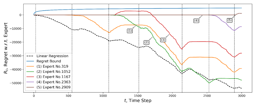
Figure 1 shows the results of the random experiment, where the graphs of $H_{t}-L^{\tau}_{t}$ present the regret of AlgorithmΒ 2 with respect to the experts starting at several time moments $\tau$.

The regret with respect to the simple linear regression performed on all data interval is also presented. We see that AlgorithmΒ 2 efficiently adapts to data and also outperforms linear regression on the entire dataset. The theoretical upper bound for the regret is also plotted (it is clear that all lines are below it).

Refer to caption
Figure 1: The graphs of the regret $R^{\tau}_{t}=H_{t}-L^{\tau}_{t}$ for the experts starting at $\tau=319,1052,1167,2363,2909$ time moments. The theoretical upper bound for the regret is represented by the line located above all the lines in the graph. The regret with respect to the simple linear regression is presented by the dotted line

5 Conclusion

In the paper we have developed the aggregating algorithm for long-term interval forecasting which is capable of combining current predictions of the experts with the outdated ones (made earlier). Combining past and current long-term forecasts allows to protects the algorithm from temporary changes in the trend of the time series, noise and outliers. Our mechanism can be applied to the time series forecasting models that are capable of predicting for the infinitely many time moments ahead, e.g. widespread ARMA-like models. For the developed algorithm we proved the sublinear $O(\ln T)$ regret bound.

We have applied PEA approach for the case of online supervised learning, where instead of point predictions, the experts and the learner present predictions in the form of regression functions. The method for smoothing regression using expert advice was presented. We consider this method of regression as a kind of long-term forecasting. Experiments conducted on synthetic data show the effectiveness of the proposed method.

Acknowledgments

The research was partially supported by the Russian Foundation for Basic Research grant 16-29-09649 ofi m.

References

  • Richardson [2007] L.Β F. Richardson, Weather prediction by numerical process, Cambridge University Press, 2007.
  • Lorenc [1986] A.Β C. Lorenc, Analysis methods for numerical weather prediction, Quarterly Journal of the Royal Meteorological Society 112Β (474) (1986) 1177–1194.
  • DeΒ Wit etΒ al. [2015] C.Β C. DeΒ Wit, F.Β Morbidi, L.Β L. Ojeda, A.Β Y. Kibangou, I.Β Bellicot, P.Β Bellemain, Grenoble traffic lab: An experimental platform for advanced traffic monitoring and forecasting [applications of control], IEEE Control Systems 35Β (3) (2015) 23–39.
  • Herrera etΒ al. [2010] J.Β C. Herrera, D.Β B. Work, R.Β Herring, X.Β J. Ban, Q.Β Jacobson, A.Β M. Bayen, Evaluation of traffic data obtained via GPS-enabled mobile phones: The Mobile Century field experiment, Transportation Research Part C: Emerging Technologies 18Β (4) (2010) 568–583.
  • Myr [2002] D.Β Myr, Real time vehicle guidance and forecasting system under traffic jam conditions, uS Patent 6,480,783, 2002.
  • Gaillard and Goude [2015] P.Β Gaillard, Y.Β Goude, Forecasting electricity consumption by aggregating experts; how to design a good set of experts, in: Modeling and stochastic learning for forecasting in high dimensions, Springer, 95–115, 2015.
  • Oliveira etΒ al. [2016] T.Β P. Oliveira, J.Β S. Barbar, A.Β S. Soares, Computer network traffic prediction: a comparison between traditional and deep learning neural networks, International Journal of Big Data Intelligence 3Β (1) (2016) 28–37.
  • Ding etΒ al. [2015] X.Β Ding, Y.Β Zhang, T.Β Liu, J.Β Duan, Deep learning for event-driven stock prediction., in: Ijcai, 2327–2333, 2015.
  • Pai and Lin [2005] P.-F. Pai, C.-S. Lin, A hybrid ARIMA and support vector machines model in stock price forecasting, Omega 33Β (6) (2005) 497–505.
  • Box etΒ al. [2015] G.Β E. Box, G.Β M. Jenkins, G.Β C. Reinsel, G.Β M. Ljung, Time series analysis: forecasting and control, John Wiley & Sons, 2015.
  • Taylor and Letham [2018] S.Β J. Taylor, B.Β Letham, Forecasting at scale, The American Statistician 72Β (1) (2018) 37–45.
  • Littlestone and Warmuth [1994] N.Β Littlestone, M.Β K. Warmuth, The Weighted Majority Algorithm, Inf. Comput. 108Β (2) (1994) 212–261, ISSN 0890-5401, URL http://dx.doi.org/10.1006/inco.1994.1009.
  • Freund and Schapire [1997] Y.Β Freund, R.Β E. Schapire, A Decision-Theoretic Generalization of On-Line Learning and an Application to Boosting, Journal of Computer and System Sciences 55Β (1) (1997) 119 – 139, ISSN 0022-0000, URL http://www.sciencedirect.com/science/article/pii/S002200009791504X.
  • Vovk [1990] V.Β G. Vovk, Aggregating Strategies, in: Proceedings of the Third Annual Workshop on Computational Learning Theory, COLT ’90, Morgan Kaufmann Publishers Inc., San Francisco, CA, USA, ISBN 1-55860-146-5, 371–386, URL http://dl.acm.org/citation.cfm?id=92571.92672, 1990.
  • Vovk [1998] V.Β Vovk, A Game of Prediction with Expert Advice, J. Comput. Syst. Sci. 56Β (2) (1998) 153–173, ISSN 0022-0000, URL http://dx.doi.org/10.1006/jcss.1997.1556.
  • Cesa-Bianchi and Lugosi [2006] N.Β Cesa-Bianchi, G.Β Lugosi, Prediction, Learning, and Games, Cambridge University Press, New York, NY, USA, ISBN 0521841089, 2006.
  • Korotin etΒ al. [2018] A.Β Korotin, V.Β V’yugin, E.Β Burnaev, Aggregating Strategies for Long-term Forecasting, arXiv preprint arXiv:1803.06727 .
  • Vovk [2001] V.Β Vovk, Competitive on-line statistics, INTERNATIONAL STATISTICAL REVIEW 69Β (2) (2001) 213–248, ISSN 0306-7734.
  • Weinberger and Ordentlich [2002] M.Β J. Weinberger, E.Β Ordentlich, On delayed prediction of individual sequences, IEEE Transactions on Information Theory 48Β (7) (2002) 1959–1976, ISSN 0018-9448.
  • Adamskiy etΒ al. [2017] D.Β Adamskiy, T.Β Bellotti, R.Β Dzhamtyrova, Y.Β Kalnishkan, Aggregating Algorithm for Prediction of Packs, CoRR abs/1710.08114, URL http://arxiv.org/abs/1710.08114.
  • Kivinen and Warmuth [1999] J.Β Kivinen, M.Β K. Warmuth, Averaging Expert Predictions, in: P.Β Fischer, H.Β U. Simon (Eds.), Computational Learning Theory, Springer Berlin Heidelberg, Berlin, Heidelberg, ISBN 978-3-540-49097-5, 153–167, 1999.
  • Blum and Mansour [2007] A.Β Blum, Y.Β Mansour, From External to Internal Regret, J. Mach. Learn. Res. 8 (2007) 1307–1324, ISSN 1532-4435, URL http://dl.acm.org/citation.cfm?id=1314498.1314543.
  • Cesa-Bianchi etΒ al. [2007] N.Β Cesa-Bianchi, Y.Β Mansour, G.Β Stoltz, Improved Second-order Bounds for Prediction with Expert Advice, Mach. Learn. 66Β (2-3) (2007) 321–352, ISSN 0885-6125, URL http://dx.doi.org/10.1007/s10994-006-5001-7.
  • Chernov and Vovk [2009] A.Β V. Chernov, V.Β Vovk, Prediction with Expert Evaluators’ Advice, in: LNCS, vol. 5809, Springer, 8–22, 2009.
  • Arce and Salinas [2012] P.Β Arce, L.Β Salinas, Online ridge regression method using sliding windows, in: Chilean Computer Science Society (SCCC), 2012 31st International Conference of the, IEEE, 87–90, 2012.
  • Bousquet and Warmuth [2003] O.Β Bousquet, M.Β K. Warmuth, Tracking a Small Set of Experts by Mixing Past Posteriors, J. Mach. Learn. Res. 3 (2003) 363–396, ISSN 1532-4435, URL http://dl.acm.org/citation.cfm?id=944919.944940.

Appendix A Auxiliary results

Vector-valued forecasts. In this paper we aggregate the vector forecasts. To do this, following [20], we apply the aggregation rule to each coordinate separately. Since the loss function is $\eta$-mixable, for any time moment $t$ for each $1\leq s\leq d$ a prediction $\gamma_{t,s}$ exists such that the inequality (6) is valid.

Let $y_{t+1},\dots,y_{t+d}$ be a sequence of outcomes. Multiplying the inequalities (10) for $s=1,\dots,d$ we obtain

eβˆ’Ξ·β€‹βˆ‘s=1dλ​(yt+s,Ξ³t,s)β‰₯∏s=1dβˆ‘n=1Nβˆ‘Ο„=1∞eβˆ’Ξ·β€‹E𝐩t,s(n,Ο„)​[λ​(yt+s,c~t,s(n,Ο„))]​w(n,Ο„),t+d.superscriptπ‘’πœ‚superscriptsubscript𝑠1π‘‘πœ†subscript𝑦𝑑𝑠subscript𝛾𝑑𝑠superscriptsubscriptproduct𝑠1𝑑superscriptsubscript𝑛1𝑁superscriptsubscript𝜏1superscriptπ‘’πœ‚subscript𝐸subscriptsuperscriptπ©π‘›πœπ‘‘π‘ delimited-[]πœ†subscript𝑦𝑑𝑠subscriptsuperscript~π‘π‘›πœπ‘‘π‘ subscriptπ‘€π‘›πœπ‘‘π‘‘\displaystyle e^{-\eta\sum_{s=1}^{d}\lambda(y_{t+s},\gamma_{t,s})}\geq\prod_{s=1}^{d}\sum_{n=1}^{N}\sum_{\tau=1}^{\infty}e^{-\eta E_{{\bf p}^{(n,\tau)}_{t,s}}[\lambda(y_{t+s},\tilde{c}^{(n,\tau)}_{t,s})]}w_{(n,\tau),t+d}. (23)

The generalized HΓΆlder inequality says that

$$\|f_{1}f_{2}\cdots f_{d}\|_{r}\leq\|f_{1}\|_{q_{1}}\|f_{2}\|_{q_{2}}\cdots\|f_{d}\|_{q_{d}},$$

where $\frac{1}{q_{1}}+\dots+\frac{1}{q_{d}}=\frac{1}{r}$, qs∈(0,+∞)subscriptπ‘žπ‘ 0q_{s}\in(0,+\infty) and fs∈Lqssubscript𝑓𝑠superscript𝐿subscriptπ‘žπ‘ f_{s}\in L^{q_{s}} for $1\leq s\leq d$. Let qs=1subscriptπ‘žπ‘ 1q_{s}=1 for all $1\leq s\leq d$, then $r=1/d$. Let

fs=eβˆ’Ξ·β€‹E𝐩t,s(n,Ο„)​[λ​(yt+s,c~t,s(n,Ο„))]subscript𝑓𝑠superscriptπ‘’πœ‚subscript𝐸subscriptsuperscriptπ©π‘›πœπ‘‘π‘ delimited-[]πœ†subscript𝑦𝑑𝑠subscriptsuperscript~π‘π‘›πœπ‘‘π‘ f_{s}=e^{-\eta E_{{\bf p}^{(n,\tau)}_{t,s}}[\lambda(y_{t+s},\tilde{c}^{(n,\tau)}_{t,s})]}

for $s=1,\dots,d$ and $\|f\|_{1}=E_{{\bf w}}(f)$, where

$${\bf w}=(w_{(n,\tau),t+d}:1\leq n\leq N,\tau\geq 1).$$

Then by HΓΆlder inequality we obtain (11).

Regret analysis. We use relative entropy as the basic tool for the regret analysis. Let $D({\bf p}\|{\bf q})=\sum\limits_{i=1}^{N}p_{i}\ln\frac{p_{i}}{q_{i}}$ be the relative entropy, where ${\bf p}=(p_{1},\dots,p_{N})$ and ${\bf q}=(q_{1},\dots,q_{N})$ are probability vectors.101010That is, $p_{i}\geq 0$, $q_{i}\geq 0$ for all $i$ and $\sum\limits_{i=1}^{N}p_{i}=1$ and $\sum\limits_{i=1}^{N}q_{i}=1$. We also define $0\ln 0=0$.

Let ${\bf l}_{t}=(l^{1}_{t},\dots,l^{N}_{t})$ be the losses of the experts at step $t$, where $1\leq i\leq N$ and $l^{i}_{t}=0$ for $1\leq t\leq d$. Let also, the evolution of the weights ${\bf w}^{\mu}_{t}$ of the experts be defined by the rule (1) and ${{\bf w}_{t+d}={\bf w}^{\mu}_{t}}$. Denote the dot product of two vectors by $({\bf q}\cdot{\bf l}_{t})$. Let also, $m_{t}=-\frac{1}{\eta}\ln\sum\limits_{i=1}^{N}w_{i,t}e^{-\eta l^{i}_{t}}$ for $t>d$.

Lemma 1.

(see [26]) For any $t>d$, and for a comparison probability vector ${\bf q}$,

$\displaystyle m_{t}=({\bf q}\cdot{\bf l}_{t})+\frac{1}{\eta}(D({\bf q}\|{\bf w}_{t})-D({\bf q}\|{\bf w}^{\mu}_{t})).$ (24)

Proof. By method (1) of the weights updating, the equality (24) is obtained as follows:

$\displaystyle m_{t}-\sum\limits_{i=1}^{N}q_{i}l^{i}_{t}=\sum\limits_{i=1}^{N}q_{i}\left(\frac{1}{\eta}\ln e^{-\eta l^{i}_{t}}+m_{t}\right)=$
$\displaystyle\frac{1}{\eta}\sum\limits_{i=1}^{N}q_{i}\left(\ln e^{-\eta l^{i}_{t}}-\ln\sum\limits_{j=1}^{N}w_{j,t}e^{-\eta l^{j}_{t}}\right)=$
$\displaystyle\frac{1}{\eta}\sum\limits_{i=1}^{N}q_{i}\ln\frac{e^{-\eta l^{i}_{t}}}{\sum\limits_{j=1}^{N}w_{j,t}e^{-\eta l^{j}_{t}}}=$
$\displaystyle\frac{1}{\eta}\sum\limits_{i=1}^{N}q_{i}\ln\frac{w^{\mu}_{i,t}}{w_{i,t}}=\frac{1}{\eta}(D({\bf q}\|w_{t})-D({\bf q}\|w^{\mu}_{t})).$
Corollary 1.

Let $T$ be a forecasting horizon and $N$ be a number of the experts. Consider the case of $d$-steps ahead prediction for $d\geq 1$. Then for any comparison vector ${\bf q}$,

$\displaystyle\sum\limits_{t=1}^{T}m_{t}-\sum\limits_{t=1}^{T}({\bf q}\cdot{\bf l}_{t})\leq\frac{1}{\eta}d\max_{1\leq i\leq N,1\leq t\leq d}\ln\frac{1}{w^{\mu}_{i,t}}.$ (25)

Proof. Summing (24) for $d+1\leq t\leq T$, we obtain

$\displaystyle\sum\limits_{t=d+1}^{T}m_{t}-\sum\limits_{t=d+1}^{T}({\bf q}\cdot{\bf l}_{t})=$
$\displaystyle\frac{1}{\eta}\sum\limits_{t=d+1}^{T}(D({\bf q}\|{\bf w}_{t})-D({\bf q}\|{\bf w}^{\mu}_{t}))=$ (26)
$\displaystyle\frac{1}{\eta}\sum\limits_{t=d+1}^{T}(D({\bf q}\|{\bf w}^{\mu}_{t-d})-D({\bf q}\|{\bf w}^{\mu}_{t}))=$ (27)
$\displaystyle\frac{1}{\eta}\sum\limits_{t=1}^{d}D({\bf q}\|{\bf w}^{\mu}_{t})\leq\frac{1}{\eta}d\max_{1\leq j\leq N,1\leq t\leq d}\ln\frac{1}{w^{\mu}_{j,t}}.$ (28)

In transition from (26) to (27) we use equality ${\bf w}_{t}={\bf w}^{\mu}_{t-d}$ for $d<t\leq T$. In transition from (27) to (28) the positive and corresponding negative terms telescope and only first $d$ positive terms remain. Also, we have used the inequality

$\displaystyle D({\bf q}\|{\bf p})=\sum\limits_{i=1}^{N}q_{i}\ln\frac{q_{i}}{p_{i}}=\sum\limits_{i=1}^{N}q_{i}\ln q_{i}+\sum\limits_{i=1}^{N}q_{i}\ln\frac{1}{p_{i}}\leq\max_{1\leq i\leq N}\ln\frac{1}{p_{i}}$

for all probability vectors ${\bf q}$ and ${\bf p}$.

Since $m_{t}=l^{i}_{t}=0$ for all $1\leq t\leq d$ and $1\leq i\leq N$, (25) follows. $\triangle$