Learning Markov Chain in Unordered Dataset

Abstract

The assumption that data samples are independently identically distributed is the backbone of many learning algorithms. Nevertheless, datasets often exhibit rich structure in practice, and we argue that there exist some unknown order within the data instances. In this technical report, we introduce OrderNet that can be used to extract the order of data instances in an unsupervised way. By assuming that the instances are sampled from a Markov chain, our goal is to learn the transitional operator of the underlying Markov chain, as well as the order by maximizing the generation probability under all possible data permutations. Specifically, we use neural network as a compact and soft lookup table to approximate the possibly huge, but discrete transition matrix. This strategy allows us to amortize the space complexity with a single model. Furthermore, this simple and compact representation also provides a short description to the dataset and generalizes to unseen instances as well. To ensure that the learned Markov chain is ergodic, we propose a greedy batch-wise permutation scheme that allows fast training. Empirically, we show that OrderNet is able to discover an order among data instances. We also extend the proposed OrderNet to one-shot recognition task and demonstrate favorable results.

1 Introduction

Recent advances in deep neural networks offer a great potential for both supervised learning, e.g., classification and regression (Glorot et al., 2011, Krizhevsky et al., 2012, Xu et al., 2015, Finn and Levine, 2017) and unsupervised learning, e.g., dimensionality reduction and density estimation (Hinton and Salakhutdinov, 2006, Vincent et al., 2010, Chen et al., 2012, Kingma and Welling, 2013, Goodfellow et al., 2014, Rasmus et al., 2015). In domains where data exhibit natural and explicit sequential structures, sequential prediction with recurrent neural networks and its variants are abundant as well, i.e., machine translation (Bahdanau et al., 2014, Sutskever et al., 2014, Wu et al., 2016), caption generation (Vinyals et al., 2015), short-text conversation (Shang et al., 2015), to name a few. However, despite the wide application of deep models in various domains, it is still unclear whether we can find implicit sequential structures in data without explicit supervision? We argue that such sequential order often exists even when dealing with the data that are naturally thought of as being $i.i.d.$ sampled from a common, perhaps complex, distribution. For example, consider a dataset consisting of the joint locations on the body of the same person taken on different days. The $i.i.d.$ assumption is justified since postures of a person taken on different days are likely unrelated. However, we can often arrange the data instances so that the joints follow an articulated motion or a set of motions in a way that makes each pose highly predictable given the previous one. Although this arrangement is individually dependent, for example, ballerina’s pose might obey different dynamics than the pose of a tennis player, the simultaneous inference on the pose dynamics can lead to a robust model that explains the correlations among joints. As another example, if we reshuffle the frames of a video clip, the data can now be modeled under the $i.i.d.$ assumption. Nevertheless, reconstructing the order leads to an alternative model where transitions between the frames are easier to fit.

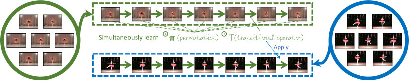
Figure 1: Illustration of the proposed model OrderNet . The data are assumed to be generated from a Markov chain, and OrderNet learns the permutation and the transition matrix simultaneously. The figure illustrates that we first train OrderNet for the data in green circles (without knowing the data order) to recover the data permutation. Then, we apply the trained transition operator to the data in blue circles to infer data permutation.

In this technical report, we investigate the following question:

Given an unordered dataset where instances may exhibit some implicit order, can we find this order in an unsupervised way?

One naive approach is to perform sorting based on a predefined distance metric, e.g., the Euclidean distance between image pixel values. However, the distance metrics have to be predefined differently according to distinct types/characteristics of the datasets at hand. A proper distance metric for one domain may not be a good one for other domains. For instance, the $p$-distance is a good measure for DNA/RNA sequences (Nei and Kumar, 2000), while it does not characterize the semantic distances between images. We argue that the key lies in the discovery of proper distance metric automatically and adaptively. Despite all kinds of interesting applications, to the best of our knowledge, we are the first to study this problem.

To approach this problem, we model the data instances by assuming that they are generated from a Markov chain. We propose to simultaneously train the transition operator and find the best order by a joint optimization over the parameter space as well as all possible permutations. We term our model OrderNet . One of the key ideas in the design of OrderNet is to use neural networks as a soft lookup table to approximate the possibly huge but discrete transition matrix, which allows OrderNet to amortize the space complexity using a unified model. Furthermore, due to the smoothness of the function approximator implemented by neural networks, the transitional operator of OrderNet can also generalize on unseen but similar data instances. To ensure the Markov chain learned by OrderNet is ergodic, we also propose a greedy batch-wise permutation scheme that allows fast training. Fig. 1 illustrates our proposed model.

As an application, we further extend our model to one-shot recognition tasks, where only one labeled data is given per category in the target domain. Most of the current work in this area focuses on learning a specific distance metric (Koch et al., 2015, Vinyals et al., 2016, Snell et al., 2017) or category-separation metric (Ravi and Larochelle, 2017, Finn et al., 2017) for the given data. During the inference phase, one would then compute either the smallest distance or highest class prediction score between the support and query instances. Alternatively, from a generative modeling perspective, we can first generate samples from the learned Markov chain, starting at each of the support instances, evaluate the query instance under the generated samples, and assign the label with the highest probability. Empirically, we demonstrate that OrderNet is able to discover implicit orders among data instances while performing comparably with many of the current state-of-the-art methods on one-shot recognition tasks.

2 The Model

We begin with introducing the setup of the problem and notations used in this technical report. Let $\{s_{i}\}_{i=1}^{n}$ denote our training data which are assumed to be generated from an unknown, fully observable, discrete time, homogeneous Markov chain $\langle\mathcal{S},\mathcal{T}\rangle$, where $\mathcal{S}$ is the state space and $\mathcal{T}$ is the transitional operator over $\mathcal{S}$, i.e., $\mathcal{T}:\mathcal{S}\to\Delta(\mathcal{S})$, a distribution over $\mathcal{S}$. In this work we assume the initial distribution is uniform over $\mathcal{S}$. Let $d=|\mathcal{S}|$ be the size of the state space. We denote the underlying data order to be a permutation over $[n]$: $\pi=\{\pi_{t}\}_{t=1}^{n}$, where $\pi_{t}$ represents the index of the instance generated at the $t$-th step of the Markov chain. Our goal is to jointly learn the transitional operator of the Markov chain as well as the most probable order of the generation process.

2.1 Parametrized Transitional Operator via Neural Networks

In classic work of learning Markov chain (Sutton and Barto, 1998), the transitional operator is usually estimated as a discrete table that maintains counts of transitions between pairs of states. However, in practice, when the state space is large, we cannot often afford to maintain the tabular transition matrix directly, which takes up to $O(d^{2})$ space. For example, if the state refers to a binary image $I\in\{0,1\}^{p}$, then $d=2^{2p}$, which is computationally intractable to maintain explicitly, even for $p$ of moderate size.

In this technical report, instead of maintaining the potentially huge discrete table, our workaround is to parametrize the transitional operator $\mathcal{T}$ as $\mathcal{T}_{\theta}(\cdot~{}|~{}\cdot):\mathcal{S}\times\mathcal{S}\to\mathbb{R}_{+}$ with learnable parameter $\theta$. Being universal function approximators (Hornik et al., 1989), neural networks could be used to efficiently approximate discrete structures which led to the recent success of deep reinforcement learning (Mnih et al., 2013, Guo et al., 2014, Oh et al., 2015, Silver et al., 2017). In our case, we use a neural network to approximate the discrete tabular transition matrix. The advantages are two-fold: first, it significantly reduces the space complexity by amortizing the space required by each separate state into a unified model. Since all the states share the same model as the transition operator, there is no need to store the transition vector for each separate state explicitly. Second, neural networks allow better generalization for the transition probabilities across states. The reason is that, in most real-world applications, states, represented as feature vectors, are not independent from each other. As a result, the differentiable approximation to a discrete structure has the additional smoothness property, which allows the transition operator to generalize on unseen states.

More specifically, $\mathcal{T}_{\theta}(s^{\prime}~{}|~{}s)$ takes two states $s$ and $s^{\prime}$ as its input and returns the corresponding (unnormalized) transition probability from $s$ to $s^{\prime}$ as follows:

$$\Pr(s^{\prime}~{}|~{}s)=\frac{1}{Z_{s}}\mathcal{T}_{\theta}(s^{\prime}~{}|~{}s),\quad Z_{s}=\sum_{s^{\prime}\in\mathcal{S}}\mathcal{T}_{\theta}(s^{\prime}~{}|~{}s)$$ (1)

where $Z_{s}$ is the normalization constant of state $s$. Note that one can consider each discrete transition matrix as a lookup table, which takes a pair of indices of the states and return the corresponding transition probability; for example, we can use $s$ and $s^{\prime}$ to locate the corresponding row and column of the table and read out its probability. From this perspective, the neural network works as a soft lookup table that outputs the unnormalized transition probability given two states (features). We will describe how to implement the transitional operator for both continuous and discrete state spaces in more detail in Sec. 2.4.

2.2 A Greedy Approximation of the Optimal Order

Given an unordered data set $\{s_{i}\}_{i=1}^{n}$, the problem of joint learning the transitional operator and the generation order can be formulated as the following maximum likelihood estimation problem:

$$\text{maximize}_{\theta,\pi}\quad\sum_{t=2}^{n}\log\mathcal{T}_{\theta}(s_{\pi_{t}}~{}|~{}s_{\pi_{t-1}})$$ (2)

where the permutation $\pi$ is chosen from all possible permutations over $[n]$. It is worth pointing out that the optimization problem (2) is intrinsically hard, as even if the true transitional operator was given, it would still be computationally intractable to find the optimal order that maximizes (2), which turns out to be an NP-hard problem.

Proposition 2.1.

Given the transitional operator $\mathcal{T}$ and a set of instances $\{s_{i}\}_{i=1}^{n}$, finding the optimal generation order $\pi$ is NP-hard.

To prove the proposition, we construct a polynomial time mapping reduction from a variant of the traveling salesman problem (TSP). To proceed, we first formally define the traveling salesman path problem (TSPP) and our optimal order problem in Markov chain (ORDER).

Definition 2.1 (TSPP).

INSTANCE: A weighted undirected graph $G=(V,E,w)$ and a constant $C$. QUESTION: Is there a Hamiltonian path in $G$ whose weight is at most $C$?

Definition 2.2 (ORDER).

INSTANCE: A Markov chain $M=\langle\mathcal{S},\mathcal{T}\rangle$, a sequence of states $X$ and a constant $p$, where $\mathcal{S}\vcentcolon=[n]$ is the set of states, $\mathcal{T}\in\mathbb{Q}_{+}^{n\times n}$ is the transitional matrix. QUESTION: Is there a permutation $\pi$ for $X$ under which $M$ generates $\pi(X)$ with probability at least $p$?

Theorem 2.1 ((Garey and Johnson, 2002)).

TSPP is NP-complete.

Theorem 2.2.

$\textsf{TSPP}\leq_{m}^{p}\textsf{ORDER}$.

Proof.

Given an instance of TSPP, $\langle G=(V,E,w),C\rangle$, we shall construct an instance of ORDER, $\langle M=\langle\mathcal{S},\mathcal{T}\rangle,X,p\rangle$ in polynomial time such that the answer to the latter is “yes” if and only if the answer to the first is also “yes”.

Given $\langle G=(V,E,w),C\rangle$, $n=|V|$, define $\Delta\vcentcolon=\max_{i\in[n]}\sum_{j=1}^{n}\exp(-w(e_{ij}))$. With $\Delta$, we construct a Markov chain $M$ where the state set is $S=V$ and the transitional matrix is defined as:

$$T_{ij}\vcentcolon=\exp(-w(e_{ij}))/\Delta,\forall e_{ij}\in E$$

and

$$T_{ii}\vcentcolon=1-\sum_{j\neq i}T_{ij}$$

Set the initial distribution of $M$ to be uniform. Choose $X=\mathcal{S}=[n]$ and $p=\exp(-C)/n\Delta^{n}$.

Now we show $\langle G=(V,E,w),C\rangle\in\textsf{TSPP}\iff\langle M=\langle V,T\rangle,\exp(-C)/n\Delta^{n}\rangle\in\textsf{ORDER}$. If $\langle G=(V,E,w),C\rangle\in\textsf{TSPP}$, then there exists a Hamiltonian path over $V$ such that the weight of the path $\leq C$. In other words, there exists a permutation $\pi$ over $V$ such that $\sum_{i=2}^{n}w(e_{\pi(i-1),\pi(i)})\leq C$, but this in turn implies:

$$\Pr(\pi(X);M)=\frac{1}{n}\prod_{i=2}^{n}\Pr(\pi(X_{i})\mid\pi(X_{i-1}))$$

$$=\frac{1}{n}\cdot\frac{\exp(\sum_{i=2}^{n}-w(e_{\pi(i-1),\pi(i)}))}{\Delta^{n}}\geq\frac{\exp(-C)}{n\Delta^{n}}=p$$

which shows $\langle M=\langle V,T\rangle,\exp(-C)/n\Delta^{n}\rangle\in\textsf{ORDER}$. The other direction is exactly the same, i.e., if we know that $\Pr(\pi(X);M)\geq\exp(-C)/n\Delta^{n}=p$, then we know that there is a Hamiltonian path in $G$ with weight $\leq C$. ∎

Corollary 2.1.

ORDER is NP-complete.

Proof.

We have proved that $\textsf{TSPP}\leq_{m}^{p}\textsf{ORDER}$. Along with the fact that TSPP is NP-complete, this shows ORDER is NP-hard. Clearly, $\textsf{ORDER}\in\textsf{NP}$ as well, because a non-deterministic machine can first guess a permutation $\pi$ and verify that $\Pr(\pi(X);M)\geq p$, which can be done in polynomial time in both $n$ and $|X|$. This finishes our proof that ORDER is NP-complete. ∎

Corollary 2.2.

Given the transitional operator $\mathcal{T}$ and a set of instances $\{s_{i}\}_{i=1}^{n}$, finding the optimal generation order $\pi$ is NP-hard.

Proof.

Since the decision version of the optimization problem is NP-complete, it immediately follows that the optimization problem is NP-hard. ∎

Given the hardness in finding the optimal order, we can only hope for an approximate solution. To this end, we propose a greedy algorithm to find an order given the current estimation of the transition operator. The algorithm is rather straightforward: it first enumerates all possible data $s_{i}$ as the first state, and then given state at time step $t-1$, it greedily finds the state at time step $t$ as the one which has the largest transition probability from the current state under the current transitional operator. The final approximate order is then defined to be the maximum of all these $n$ orders. We list the pseudocode in Alg. 1. This algorithm has time complexity $O(n^{3})$. To reduce the complexity for large $n$, we can uniformly at random sample a data to be the one generated at the first time step, and again using greedy search to compute an approximate order. This helps to reduce the complexity to $O(n^{2})$. Note that more advanced heuristics exist for finding the approximate order $\pi$, e.g., the genetic algorithm, simulated annealing, tabu search, to name a few.

Algorithm 1 Greedy Approximate Order

0:  Input data $\{s_{i}\}_{i=1}^{n}$ and transitional operator $\mathcal{T}_{\theta}(s^{\prime}~{}|~{}s)$.

1:  for $i=1$ to $n$ do

2:     $\pi_{1}^{(i)}\leftarrow i$

3:     for $j=2$ to $n$ do

4:        $\pi_{j}^{(i)}\leftarrow\max_{k\not\in\pi^{(i)}_{1:j-1}}\mathcal{T}_{\theta}(s_{k}~{}|~{}s_{\pi^{(i)}_{j-1}})$// greedy selection

5:     end for

6:  end for

7:  $\hat{\pi}\leftarrow\operatorname*{arg\,max}_{i\in[n]}\sum_{t=2}^{n}\log\mathcal{T}_{\theta}(s_{\pi^{(i)}_{t-1}}~{}|~{}s_{\pi^{(i)}_{t}})$

Using Alg. 1 as a subroutine, at a high level, the overall optimization algorithm can be understood as an instance of coordinate ascent, where we alternatively optimize over the transitional operator $\mathcal{T}_{\theta}$ and the approximate order of the data $\hat{\pi}$. Given $\hat{\pi}$, we can optimize $\theta$ by gradient ascent. In what follows, we introduce a batch-wise permutation training scheme to further reduce the complexity of Alg. 1 when $n$ is large, so that is scales linearly with $n$.

2.3 Batch-Wise Permutation Training

The $O(n^{3})$ computation to find the approximate order in Alg. 1 can still be expensive when the size of the data is large. In this section we provide batch-wise permutation training to avoid this issue. The idea is to partition the original training set into batches with size $b$ and perform greedy approximate order on each batch. Assuming $b\ll n$ is a constant, the effective time complexity becomes: $O(b^{3})\cdot n/b=O(nb^{2})$, which is linear in $n$.

However, since training data are partitioned into chunks, the learned transition operator is not guaranteed to have nonzero transition probabilities between data from different chunks. In other words, the learned transition operator does not necessarily induce an ergodic Markov chain due to the isolated chuck of states, which corresponds to disconnected components of the transition graph. To avoid this problem, we use a simple strategy to enforce that some samples overlap between the consecutive batches. We show the pseudocode in Alg. 2, where $b$ means the batch size, $\gamma$ is the learning rate and $b_{0}<b$ is the number of overlapping states between consecutive batches.

Algorithm 2 Batch-Wise Permutation Training

0:  $\{s_{i}\}_{i=1}^{n}$, $b_{0}$, $b$, $t$, $\gamma$

1:  Initialize $\theta^{(0)}$, $\{x^{(0)}_{i}\}_{i=1}^{b}$

2:  for $k=1$ to $\infty$ do

3:     if $k\equiv 1(\mathrm{mod}\,\,t)$ then

4:        Sample $\{x^{(k)}_{i}\}_{i=1}^{b-b_{0}}\sim\{s_{i}\}_{i=1}^{n}$

5:        $\{x^{(k)}_{i}\}_{i=1}^{b}\leftarrow\{x^{(k)}_{i}\}_{i=1}^{b-b_{0}}\cup\{x^{(k-1)}_{i}\}_{i=1}^{b_{0}}$// construct overlapping states

6:     end if

7:     Compute $\hat{\pi}^{(k)}$ using the Greedy Approximate Order (Alg. 1) on $\{x^{(k)}_{i}\}_{i=1}^{b}$

8:     Compute $\nabla^{(k-1)}_{\theta}\log\Pr(\{x_{i}\}_{i=1}^{b};\theta^{(k-1)},\hat{\pi}^{(k)})$

9:     $\theta^{(k)}=\theta^{(k-1)}+\gamma\nabla^{(k-1)}_{\theta}\log\Pr(\{x_{i}\}_{i=1}^{b};\theta^{(k-1)},\hat{\pi}^{(k)})$// update of transitional operator

10:  end for

2.4 Explicit Transitional Operator

We now provide a detailed description on how to implement and parametrize the transitional operator. The proposed transitional operator works for both discrete and continuous state space, which we discuss separately. Note that different from previous work (Song et al., 2017), where the only requirement for the transitional operator is a good support of efficient sampling, in our setting, we need to form explicit transitional operator that allows us to evaluate the probability density or mass of transitions. We call such parametrized transitional operators as explicit transitional operators, to distinguish them from previous implicit ones.

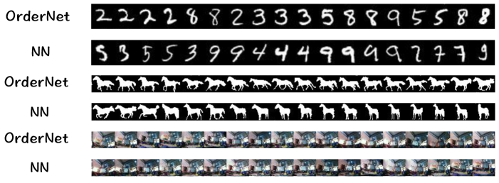
Figure 2: The implicit order observed from OrderNet and the order implied from Nearest Neighbor sorting on MNIST, Horse, and MSR-SenseCam datasets.

Continuous state space. Let state $s\in\mathbb{R}^{p}$ be a $p$-dimensional feature vector. In this case we assume that $s^{\prime}\sim\mathcal{N}(m_{\theta}(s),v_{\theta}(s))$, where both the mean and the variance of the normal distribution are implemented with neural networks. Similar ideas on parametrizing the mean and variance functions of the normal distribution have recently been widely applied, e.g., variational autoencoder (VAE) (Kingma and Welling, 2013) and its variants, etc. Under this model the evaluation of the transitional operator becomes:

$$\begin{split}&\log\mathcal{T}_{\theta}(s^{\prime}~{}|~{}s)\propto\\ &-\frac{1}{2}(s^{\prime}-m_{\theta}(s))^{T}v^{-1}_{\theta}(s)(s^{\prime}-m_{\theta}(s))-\log\det(v_{\theta}(s))\end{split}$$ (3)

In practice, due to the large $O(p^{2})$ space complexity of learning a full covariance matrix, we further assume that the covariance is diagonal. This allows us to further simplify the last term (3) as $\mathbf{1}_{p}^{T}\log v_{\theta}(s)$.

Discrete state space. Let state $s\in\{0,1\}^{p}$ be a $p$-dimensional 0-1 vector. Without any assumption, the distribution has a support of size $O(2^{p})$, which is intractable to maintain exactly. To avoid this issue, again, we adopt the conditional independence assumption for $\mathcal{T}_{\theta}(s^{\prime}~{}|~{}s)$, i.e.,

$$\begin{split}&\log\mathcal{T}_{\theta}(s^{\prime}~{}|~{}s)=\log\prod_{j=1}^{p}\Pr(s^{\prime}_{j}~{}|~{}s;\theta)\vcentcolon=\\ &\sum_{j=1}^{p}s^{\prime}_{j}\cdot\log f_{\theta,j}(s)+(1-s^{\prime}_{j})\cdot\log(1-f_{\theta,j}(s))\end{split}$$ (4)

where $f_{\theta,j}(\cdot)$ is the $j$-th network with sigmoid output so that we can guarantee $f_{\theta,j}(\cdot)\in(0,1)$, representing the probability $\Pr(s^{\prime}_{j}=1~{}|~{}s;\theta)$. In practice, the networks $\{f_{\theta,j}\}_{j=1}^{p}$ share all the feature transformation layers, except the last layer where each $f_{\theta,j}$ has its own sigmoid layer. Such design not only allows potential feature transfer/multitask learning among $p$ output variables, but also improves generalization by substantially reducing model size. Interestingly, the proposed operator shares many connections with the classic restricted Boltzmann machine (RBM) (Hinton and Salakhutdinov, 2006), where both models assume conditional independence at the output layer. On ther other hand, RBM is a shallow log-linear model, whereas the proposed operator allows flexible design with various deep architectures (Nair and Hinton, 2010), and the only requirement is that the output layer is sigmoidal.

As a concluding remark of this section, we note that a common assumption in designing the explicit transitional operators for both continuous and discrete state space models is that the probability density/mass decomposes in the output layer. Such assumption is introduced mainly due to the intractable space requirement on maintaining the explicit density/mass for optimization in (2). While such assumption is strong, we empirically find in our experiments the proposed models are still powerful in discovering orders from datasets, due to the deep and flexible architectures used as feature transformation.

3 Experiments

In this section, we first qualitatively evaluate OrderNet on MNIST (LeCun et al., 1990), Horse (Borenstein and Ullman, 2002), and MSR-SenseCam (Jojic et al., 2010) datasets (in which data were assumed to be i.i.d.) to discover their implicit orders. Next, we will use UCF-CIL-Action dataset (Shen and Foroosh, 2008) (with order information) to quantitatively evaluate OrderNet and its generalization ability. Last, we apply our OrderNet on miniImageNet (Vinyals et al., 2016, Ravi and Larochelle, 2017) dataset for one-shot image recognition task.

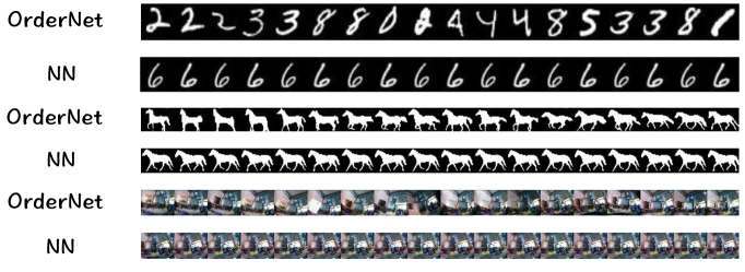
Figure 3: Image propagation for OrderNet and Nearest Neighbor search on MNIST, Horse, and MSR-SenseCam datasets.

3.1 Discovering Implicit Order

MNIST. MNIST is a well-studied dataset that contains 60,000 training examples. Each example is a digit image with size 28x28. We rescale the pixel values to $[0,1]$. Note that since MNIST contains a large number of instances, we perform the ordering in a randomly sampled batch to demonstrate our results.

Horse. The Horse dataset consists of $328$ horse images collected from the Internet. Each horse is centered in a 30x40 image. For the preprocessing, the author applied foreground-background segmentation and set the pixel value to $1$ and $0$ for object and background, respectively. Examples are show in the supplement.

MSR-SenseCam. MSR-SenseCam is a dataset consisting of images taken by SenseCam wearable camera. It contains $45$ classes with approximately $150$ images per class. Each image has size 480x640. We resize each image into 224x224 and extract the feature from VGG-19 network (Simonyan and Zisserman, 2014). In this dataset, we consider only office category, which has $362$ images.

3.1.1 Implicit Orders

We apply Alg. 2 to train OrderNet . When the training converges, we plot the images following the recovered permutation $\hat{\pi}$. Note that $\hat{\pi}$ can be seen as the implicit order suggested by OrderNet . For comparison, we also plot the images following nearest neighbor (NN) sorting using Euclidean distances. Hyper-parameters and network architectures for parameterizing the transitional operators are specified in the supplement. The results are shown in Fig. 2. We first observe that consecutive frames in the order extracted by the OrderNet have visually high autocorrelation, implying that OrderNet can discover some implicit order for these dataset. On the other hand, it is hard to qualitatively compare the results with Nearest Neighbor’s. To address this problem, we perform another evaluation in the following subsection and also perform quantitative analysis in Sec. 3.2.

3.1.2 Image Propagation

To verify that our proposed model can automatically learn order, we first describe an evaluation mtric, which we term as image propagation, defined as follows. Given an image $s$, the propagated image

$$s^{\prime}=\operatorname*{arg\,max}_{\hat{s}\in\{s_{i}\}_{i=1}^{n}\setminus s}\mathcal{T}_{\theta}(\hat{s}~{}|~{}s),$$

i.e., the most probable next image given by the transitional operator. Similar to Sec. 3.1.1, we exploit NN search using Euclidean distance for comparison. Precisely,

$$s^{\prime}_{NN}=\operatorname*{arg\,min}_{\hat{s}\in\{s_{i}\}_{i=1}^{n}\setminus s}||s-\hat{s}||.$$

Fig. 3 illustrates the image propagation of OrderNet and NN search. We can see that NN search would stick between two similar images. On the other hand, OrderNet shows a series of images with consecutive actions. This implies the distinction between the discriminative (sampling by a fixed distance metric) and the generative (sampling through the transition operator in a Markov chain) model.

3.2 Recovering Orders in Ordered Datasets

UCF-CIL-Action. UCF-CIL-Action (Shen and Foroosh, 2008) is a dataset containing different action videos by various subjects, distinct cameras, and diverse viewpoints. In addition to videos, the dataset also provides $11$ tracking points (presented in $x$ and $y$ axis) for head, right shoulder, right elbow, right hand, left shoulder, left elbow, left hand, right knee, right foot, left knee, and left foot. We represent a frame by concatenating $11$ tracking points at the end of pre-extracted features from VGG-19 network. In this dataset, we select ballet fouette actions to evaluate OrderNet . Details about this experiment, including hyperparameters, model architecture, and additional experiments on the tennis serve actions, are all provided in the supplement. To quantitatively study the quality of the recovered permutation, we use Kendall Tau-b correlation score (Kendall et al., 1946) to measure the distance between two permutations, which outputs the value from $-1$ to $1$. The larger the Kendal Tau-b, the more similar the two permutations are. If Kendal Tau-b value is $1$, two permutations are exactly the same. In the following, we evaluate OrderNet under two settings: (1) train OrderNet and evaluate the order for the same subject, and (2) train OrderNet from one subject but evaluate on the different subjects. To simulate the groundtruth ordering, we took a video sequence and then reshuffle its frames, and use OrderNet / NN to reconstruct the order. The results are reported for random $20$ trials with mean and standard deviation.

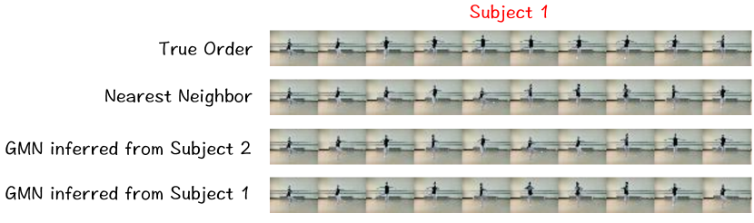
Figure 4: Ballet fouette action for $\mathsf{subject1}$ with : (a) true order, (b) order recovered from Nearest Neighbor, (c) order recovered from OrderNet trained on different subject, and (d) order recovered from OrderNet trained on the same subject. Only partial orders are shown.

Table 1: Kendall Tau-b score between the true order and the recovered orders from OrderNet / NN with Euclidean distance. OrderNet are trained on different subjects with ballet fouette actions.

Applied To	Trained OrderNet On				$\mathsf{NN}$
	$\mathsf{Subject\,\,1}$	$\mathsf{Subject\,\,2}$	$\mathsf{Subject\,\,3}$	$\mathsf{Subject\,\,4}$
$\mathsf{Subject\,\,1}$	0.364 $\pm$ 0.058	0.183 $\pm$ 0.033	0.247 $\pm$ 0.052	0.200 $\pm$ 0.065	0.137
$\mathsf{Subject\,\,2}$	0.062 $\pm$ 0.091	0.085 $\pm$ 0.038	0.079 $\pm$ 0.035	0.074 $\pm$ 0.052	-0.217
$\mathsf{Subject\,\,3}$	-0.026 $\pm$ 0.072	-0.086 $\pm$ 0.066	0.191 $\pm$ 0.055	-0.092 $\pm$ 0.083	-0.122
$\mathsf{Subject\,\,4}$	0.274 $\pm$ 0.056	0.288 $\pm$ 0.032	0.304 $\pm$ 0.025	0.355 $\pm$ 0.025	0.292

In Table 1, we report the Kendall Tau-b values between the true order and the recovered order from OrderNet / NN. Qualitative results are shown in Fig. 4. First of all, we observe that OrderNet can recover more accurate orders than NN according to higher Kendall Tau-b values. The most accurate order can be recovered when the OrderNet was trained on the same subject for evaluation (diagonal in Table 1). Next, we examine the generalization ability of OrderNet . In most of the cases, when we apply the trained OrderNet to different subjects, we can achieve higher Kendall Tau-b values comparing to NN, with only two exceptions. This result implies that OrderNet can generalize from one subject to another.

3.3 One-Shot Recognition

MiniImageNet. MiniImageNet is a benchmark dataset designed for evaluation of one-shot learning (Vinyals et al., 2016, Ravi and Larochelle, 2017). Being a subset of ImageNet (Russakovsky et al., 2015), it contains $100$ classes and each class has $600$ images. Each image is downsampled to size 84x84. As suggested in (Ravi and Larochelle, 2017), the dataset is divided into three parts: $64$ classes for training, $16$ classes for validation, and $20$ classes for testing.

Same as (Ravi and Larochelle, 2017), in this experiment we consider the $5-$way $1-$shot problem. That is, from testing classes, we sample $5$ classes with each class containing $1$ labeled example. The labeled examples are referred as support instances. Then, we randomly sample $500$ unlabeled query examples in these $5$ classes for evaluation. In more detail, we train OrderNet on training classes and then apply it to testing classes. For each training episode, we sample $1$ class from the training classes and let $\{s_{i}\}_{i=1}^{n}$ be all the data from this class. We consider $3,000$ training episodes. On the other hand, for each testing episode, we apply OrderNet to generate a chain from each support instance:

$$\tilde{s}_{1}^{c}\sim\mathcal{T}_{\theta}(\cdot~{}|~{}s_{0}^{c}),\ldots,\tilde{s}_{k}^{c}\sim\mathcal{T}_{\theta}(\cdot~{}|~{}\tilde{s}_{k-1}^{c}),$$

where $s_{0}^{c}$ is the support instance belonging to class $c$ and $\tilde{s}^{c}$ is the generated samples from the Markov chain. Next, we fit each query example into each chain by computing the average approximating log-likelihood. Namely, the log-probability for generating the query sample $s_{q}$ in the chain of class $c$ is

$$\log\Pr(s_{q}|c)\vcentcolon=(\mathrm{log}\mathcal{T}_{\theta}(s_{q}~{}|~{}s_{0}^{c})+\sum_{i=1}^{k}\log\mathcal{T}_{\theta}(s_{q}~{}|~{}\tilde{s}_{i}^{c}))/(k+1).$$

In a generative viewpoint, the predicted class $\hat{c}$ for $s_{q}$ is determined by

$$\hat{c}=\operatorname*{arg\,max}_{c}\log\Pr(s_{q}|c).$$

We repeat this procedure for $10,000$ times and report the average with $95\%$ confidence intervals in Table 2.

For fair comparisons, we use the same architecture specified in (Ravi and Larochelle, 2017) to extract $1600$-dimensional features. We pretrain the architecture using standard softmax regression on image-label pairs in training and validation classes. The architecture consists of $4$ blocks. Each block comprises a CNN layer with $64$ $3$x$3$ convolutional filters, Batch Normalization (Ioffe and Szegedy, 2015) layer, ReLU activation, and $2$x$2$ Max-Pooling layer. Then, we train OrderNet based on these $1,600$ dimensional features. More details can be found in the supplement.

Table 2: 5-way 1-shot recognition task for miniImageNet. We report the mean in $10,000$ episodes with $95\%$ confidence interval.

Model	Accuracy
Meta-Learner LSTM (Ravi and Larochelle, 2017)	43.44$\pm$0.77
Model-Agnostic Meta-Learning (Finn et al., 2017)	48.70$\pm$1.84
Meta-SGD (Li et al., 2017)	50.47$\pm$1.87
Nearest Neighbor with Cosine Distance	41.08$\pm$0.70
Matching Networks FCE (Vinyals et al., 2016)	43.56$\pm$0.84
Siamese (Koch et al., 2015)	48.42$\pm$0.79
mAP-Direct Loss Minimization (Triantafillou et al., 2017)	41.64$\pm$0.78
mAP-Structural Support Vector Machine (Triantafillou et al., 2017)	47.89$\pm$0.78
Prototypical Networks (Snell et al., 2017)	49.42$\pm$0.78
OrderNet	45.36$\pm$0.94

3.3.1 Results

We compare OrderNet and the related approaches in Table 2, in which we consider only the approaches (Ravi and Larochelle, 2017, Finn and Levine, 2017, Li et al., 2017, Vinyals et al., 2016, Koch et al., 2015, Triantafillou et al., 2017, Snell et al., 2017) using same architecture design (i.e., 4 layers CNN) in (Ravi and Larochelle, 2017). First, we compare OrderNet with meta-learning based methods. The best result is reported by Meta-SGD (Li et al., 2017) with $50.47\pm 1.87$. Although OrderNet suffers from the performance drop, it requires a much less computational budget. The reason is that the meta-learning approaches (Ravi and Larochelle, 2017, Finn et al., 2017, Munkhdalai and Yu, 2017, Li et al., 2017, Mishra et al., 2017) rely on huge networks to manage complicated intersections between meta and base learners, while parameters for OrderNet exist only in $\theta$ which is a relatively tiny network. On the other hand, the best performance reported in the distance-metric based approaches is the Prototypical Networks (Snell et al., 2017) with $49.42\pm 0.78$. As a comparison, OrderNet enjoys more flexibility without the need of defining any distance metric as in (Vinyals et al., 2016, Koch et al., 2015, Triantafillou et al., 2017, Snell et al., 2017, Shyam et al., 2017, Mehrotra and Dukkipati, 2017).

4 Related Work

In this section, we provide brief discussions on related generative models in deep learning. In general, deep generative models can be categorized into two classes: explicit models and implicit models (Goodfellow, 2016). In explicit models, probability density or mass functions are explicitly defined, often parametrized with deep neural networks, so that the models can be learned or trained with statistical principles, e.g., maximum likelihood estimation or maximum a posteriori. Typical examples include variational autoencoder and its various variants (Kingma and Welling, 2013). As a comparison, implicit models do not provide a way for probability density/mass evaluation. Instead, the focus of implicit models lies in efficient sampling. This includes the popular generative adversarial networks (Goodfellow et al., 2014) and its family. Without explicit density definitions, implicit models often rely on external properties of the model for training, including finding Nash equilibrium of the zero-sum game (Goodfellow et al., 2014), mixing distribution of the Markov chain (Song et al., 2017, Bordes et al., 2017), etc. Using this taxonomy, our approach can be understood as an explicit generative model with well-defined probability density/mass functions. Compared with previous works in this line of research, OrderNet has two significant improvements: first, existing works often assume training instances are $i.i.d.$ sampled from a fixed, probably unknown, distribution. On the other hand, we assume the data are sequentially generated from a Markov in an unknown order. Our model can thus discover the order and help us understand the implicit data relationships. Second, prior approaches were proposed based on the notion of denoising models. In other words, their goal was generating high-quality samples (Kingma and Welling, 2013). As a contrast, we aim at learning the dynamics of the chain whle at the same time recovering the order as well.

5 Conclusion

In this technical report, we propose OrderNet that can simultaneously learn the dynamics of a Markov chain and the generation order of data instances sampled from this chain. Our model is equipped with explicit, well-defined generative probabilities so that we can use statistical principles to train our model. Compared with previous work, OrderNet uses flexible neural networks to parametrize the transitonal operator so that it amortizes the space complexity of the state space (only depends on the dimension of the state space, but not its cardinality), while at the same time achieves good generalization on unseen states during training. Experiments on discovering orders from unordered datasets validate the effectiveness of our model. As an application, we also extend our model to one-shot learning, showing that it performs comparably with state-of-the-art models, but with much less computational resources.

References

- Bahdanau et al. (2014) Dzmitry Bahdanau, Kyunghyun Cho, and Yoshua Bengio. Neural machine translation by jointly learning to align and translate. arXiv preprint arXiv:1409.0473, 2014.
- Bordes et al. (2017) Florian Bordes, Sina Honari, and Pascal Vincent. Learning to generate samples from noise through infusion training. arXiv preprint arXiv:1703.06975, 2017.
- Borenstein and Ullman (2002) Eran Borenstein and Shimon Ullman. Class-specific, top-down segmentation. In European conference on computer vision, pages 109–122. Springer, 2002.
- Chen et al. (2012) Minmin Chen, Zhixiang Xu, Kilian Weinberger, and Fei Sha. Marginalized denoising autoencoders for domain adaptation. arXiv preprint arXiv:1206.4683, 2012.
- Finn and Levine (2017) Chelsea Finn and Sergey Levine. Deep visual foresight for planning robot motion. In Robotics and Automation (ICRA), 2017 IEEE International Conference on, pages 2786–2793. IEEE, 2017.
- Finn et al. (2017) Chelsea Finn, Pieter Abbeel, and Sergey Levine. Model-agnostic meta-learning for fast adaptation of deep networks. arXiv preprint arXiv:1703.03400, 2017.
- Garey and Johnson (2002) Michael R Garey and David S Johnson. Computers and intractability, volume 29. wh freeman New York, 2002.
- Glorot et al. (2011) Xavier Glorot, Antoine Bordes, and Yoshua Bengio. Domain adaptation for large-scale sentiment classification: A deep learning approach. In Proceedings of the 28th international conference on machine learning (ICML-11), pages 513–520, 2011.
- Goodfellow (2016) Ian Goodfellow. Nips 2016 tutorial: Generative adversarial networks. arXiv preprint arXiv:1701.00160, 2016.
- Goodfellow et al. (2014) Ian Goodfellow, Jean Pouget-Abadie, Mehdi Mirza, Bing Xu, David Warde-Farley, Sherjil Ozair, Aaron Courville, and Yoshua Bengio. Generative adversarial nets. In Advances in neural information processing systems, pages 2672–2680, 2014.
- Guo et al. (2014) Xiaoxiao Guo, Satinder Singh, Honglak Lee, Richard L Lewis, and Xiaoshi Wang. Deep learning for real-time atari game play using offline monte-carlo tree search planning. In Advances in neural information processing systems, pages 3338–3346, 2014.
- Hinton and Salakhutdinov (2006) Geoffrey E Hinton and Ruslan R Salakhutdinov. Reducing the dimensionality of data with neural networks. science, 313(5786):504–507, 2006.
- Hornik et al. (1989) Kurt Hornik, Maxwell Stinchcombe, and Halbert White. Multilayer feedforward networks are universal approximators. Neural networks, 2(5):359–366, 1989.
- Ioffe and Szegedy (2015) Sergey Ioffe and Christian Szegedy. Batch normalization: Accelerating deep network training by reducing internal covariate shift. In International Conference on Machine Learning, pages 448–456, 2015.
- Jojic et al. (2010) Nebojsa Jojic, Alessandro Perina, and Vittorio Murino. Structural epitome: a way to summarize one’s visual experience. In J. D. Lafferty, C. K. I. Williams, J. Shawe-Taylor, R. S. Zemel, and A. Culotta, editors, Advances in Neural Information Processing Systems 23, pages 1027–1035. Curran Associates, Inc., 2010. URL http://papers.nips.cc/paper/4092-structural-epitome-a-way-to-summarize-ones-visual-experience.pdf.
- Kendall et al. (1946) Maurice George Kendall et al. The advanced theory of statistics. The advanced theory of statistics., (2nd Ed), 1946.
- Kingma and Welling (2013) Diederik P Kingma and Max Welling. Auto-encoding variational bayes. arXiv preprint arXiv:1312.6114, 2013.
- Koch et al. (2015) Gregory Koch, Richard Zemel, and Ruslan Salakhutdinov. Siamese neural networks for one-shot image recognition. In ICML Deep Learning Workshop, volume 2, 2015.
- Krizhevsky et al. (2012) Alex Krizhevsky, Ilya Sutskever, and Geoffrey E Hinton. Imagenet classification with deep convolutional neural networks. In Advances in neural information processing systems, pages 1097–1105, 2012.
- LeCun et al. (1990) Yann LeCun, Bernhard E Boser, John S Denker, Donnie Henderson, Richard E Howard, Wayne E Hubbard, and Lawrence D Jackel. Handwritten digit recognition with a back-propagation network. In Advances in neural information processing systems, pages 396–404, 1990.
- Li et al. (2017) Zhenguo Li, Fengwei Zhou, Fei Chen, and Hang Li. Meta-sgd: Learning to learn quickly for few shot learning. arXiv preprint arXiv:1707.09835, 2017.
- Mehrotra and Dukkipati (2017) Akshay Mehrotra and Ambedkar Dukkipati. Generative adversarial residual pairwise networks for one shot learning. arXiv preprint arXiv:1703.08033, 2017.
- Mishra et al. (2017) Nikhil Mishra, Mostafa Rohaninejad, Xi Chen, and Pieter Abbeel. Meta-learning with temporal convolutions. arXiv preprint arXiv:1707.03141, 2017.
- Mnih et al. (2013) Volodymyr Mnih, Koray Kavukcuoglu, David Silver, Alex Graves, Ioannis Antonoglou, Daan Wierstra, and Martin Riedmiller. Playing atari with deep reinforcement learning. arXiv preprint arXiv:1312.5602, 2013.
- Munkhdalai and Yu (2017) Tsendsuren Munkhdalai and Hong Yu. Meta networks. arXiv preprint arXiv:1703.00837, 2017.
- Nair and Hinton (2010) Vinod Nair and Geoffrey E Hinton. Rectified linear units improve restricted boltzmann machines. In Proceedings of the 27th international conference on machine learning (ICML-10), pages 807–814, 2010.
- Nei and Kumar (2000) Masatoshi Nei and Sudhir Kumar. Molecular evolution and phylogenetics. Oxford university press, 2000.
- Oh et al. (2015) Junhyuk Oh, Xiaoxiao Guo, Honglak Lee, Richard L Lewis, and Satinder Singh. Action-conditional video prediction using deep networks in atari games. In Advances in Neural Information Processing Systems, pages 2863–2871, 2015.
- Rasmus et al. (2015) Antti Rasmus, Mathias Berglund, Mikko Honkala, Harri Valpola, and Tapani Raiko. Semi-supervised learning with ladder networks. In Advances in Neural Information Processing Systems, pages 3546–3554, 2015.
- Ravi and Larochelle (2017) Sachin Ravi and Hugo Larochelle. Optimization as a model for few-shot learning. ICLR, 2017.
- Russakovsky et al. (2015) Olga Russakovsky, Jia Deng, Hao Su, Jonathan Krause, Sanjeev Satheesh, Sean Ma, Zhiheng Huang, Andrej Karpathy, Aditya Khosla, Michael Bernstein, et al. Imagenet large scale visual recognition challenge. International Journal of Computer Vision, 115(3):211–252, 2015.
- Shang et al. (2015) Lifeng Shang, Zhengdong Lu, and Hang Li. Neural responding machine for short-text conversation. arXiv preprint arXiv:1503.02364, 2015.
- Shen and Foroosh (2008) Yuping Shen and Hassan Foroosh. View-invariant action recognition using fundamental ratios. In Computer Vision and Pattern Recognition, 2008. CVPR 2008. IEEE Conference on, pages 1–6. IEEE, 2008.
- Shyam et al. (2017) Pranav Shyam, Shubham Gupta, and Ambedkar Dukkipati. Attentive recurrent comparators. arXiv preprint arXiv:1703.00767, 2017.
- Silver et al. (2017) David Silver, Julian Schrittwieser, Karen Simonyan, Ioannis Antonoglou, Aja Huang, Arthur Guez, Thomas Hubert, Lucas Baker, Matthew Lai, Adrian Bolton, et al. Mastering the game of go without human knowledge. Nature, 550(7676):354, 2017.
- Simonyan and Zisserman (2014) Karen Simonyan and Andrew Zisserman. Very deep convolutional networks for large-scale image recognition. arXiv preprint arXiv:1409.1556, 2014.
- Snell et al. (2017) Jake Snell, Kevin Swersky, and Richard S Zemel. Prototypical networks for few-shot learning. arXiv preprint arXiv:1703.05175, 2017.
- Song et al. (2017) Jiaming Song, Shengjia Zhao, and Stefano Ermon. A-nice-mc: Adversarial training for mcmc. In Advances in Neural Information Processing Systems, pages 5146–5156, 2017.
- Sutskever et al. (2014) Ilya Sutskever, Oriol Vinyals, and Quoc V Le. Sequence to sequence learning with neural networks. In Advances in neural information processing systems, pages 3104–3112, 2014.
- Sutton and Barto (1998) Richard S Sutton and Andrew G Barto. Reinforcement learning: An introduction, volume 1. MIT press Cambridge, 1998.
- Triantafillou et al. (2017) Eleni Triantafillou, Richard Zemel, and Raquel Urtasun. Few-shot learning through an information retrieval lens. arXiv preprint arXiv:1707.02610, 2017.
- Vincent et al. (2010) Pascal Vincent, Hugo Larochelle, Isabelle Lajoie, Yoshua Bengio, and Pierre-Antoine Manzagol. Stacked denoising autoencoders: Learning useful representations in a deep network with a local denoising criterion. Journal of Machine Learning Research, 11(Dec):3371–3408, 2010.
- Vinyals et al. (2015) Oriol Vinyals, Alexander Toshev, Samy Bengio, and Dumitru Erhan. Show and tell: A neural image caption generator. In Computer Vision and Pattern Recognition (CVPR), 2015 IEEE Conference on, pages 3156–3164. IEEE, 2015.
- Vinyals et al. (2016) Oriol Vinyals, Charles Blundell, Tim Lillicrap, Daan Wierstra, et al. Matching networks for one shot learning. In Advances in Neural Information Processing Systems, pages 3630–3638, 2016.
- Wu et al. (2016) Yonghui Wu, Mike Schuster, Zhifeng Chen, Quoc V Le, Mohammad Norouzi, Wolfgang Macherey, Maxim Krikun, Yuan Cao, Qin Gao, Klaus Macherey, et al. Google’s neural machine translation system: Bridging the gap between human and machine translation. arXiv preprint arXiv:1609.08144, 2016.
- Xu et al. (2015) Kelvin Xu, Jimmy Ba, Ryan Kiros, Kyunghyun Cho, Aaron Courville, Ruslan Salakhudinov, Rich Zemel, and Yoshua Bengio. Show, attend and tell: Neural image caption generation with visual attention. In International Conference on Machine Learning, pages 2048–2057, 2015.