Accessing Masses Beyond Collider Reach - in EFT

Abstract

We demonstrate how masses of new states, beyond direct experimental reach, could nevertheless be extracted in the framework of effective field theory (EFT), given broad assumptions on the underlying UV physics, however not sticking to a particular setup nor fixing the coupling strength of the scenario. The flat direction in the $g_{\ast}$ vs. $M$ plane is lifted by studying correlations between observables that depend on operators with a different $\hbar$ scaling. We discuss the remaining model dependence (which is inherent even in the EFT approach to have control over the error due to the truncation of the power series), as well as prospects to test paradigms of UV physics. In particular, we provide an assessment of which correlations are best suited regarding sensitivity, give an overview of possible/expected effects in different observables, and demonstrate how perturbativity and direct search limits corner possible patterns of deviations from the SM in a given UV paradigm.

1 General Introduction

Given the clear technical limitations in increasing the energy of collider experiments, it is important to try to access the properties of physics beyond the Standard Model (BSM) indirectly via precise measurements of observables at available energies. However, this approach features in general a significant limitation, since new degrees of freedom, entering as virtual particles in processes with characteristic energy scales below their production threshold, generically lead to corrections scaling like a ratio of their coupling and their mass. Acquiring information about their actual mass spectrum requires usually very specific assumptions about the coupling strength - which in reality however could span a huge range from very weak coupling $g_{\ast}\ll 1$ up to strong coupling, like $g_{\ast}\lesssim 4\pi$. In this paper we point out how the different $\hbar$ scaling of various operators can be used to lift flat directions in the coupling vs. mass plane by examining more than one observable at a time, thus allowing to estimate systematically at which mass the new physics (NP) actually can be expected.

The framework used for this analysis is the effective field theory (EFT) extension of the SM, which is indeed the most general parametrization of NP that resides at energies much larger than both the electroweak scale $M_{\rm EW}$ and the characteristic scale $E$ probed by the experiment of interest. It can be fully formulated in terms of low mass (SM) fields, while the effect of the NP will manifest itself in the presence of operators with mass dimension $D>4$ in the effective Lagrangian Buchmuller:1985jz ; Hagiwara:1993ck ; Grzadkowski:2010es

$${\cal L}_{\rm{eff}}={\cal L}_{\rm SM}+\sum_{i}c_{i}^{(6)}{\cal O}_{i}^{(6)}\ +\sum_{j}c_{j}^{(8)}{\cal O}_{j}^{(8)}+\cdots\,,$$ (1)

where ${\cal L}_{\rm SM}$ is the SM Lagrangian, and we have assumed baryon and lepton number conservation. The operators ${\cal O}_{i}^{(D)}$ of canonical dimension $D$ consist of all (Poincaré invariant and hermitian) combinations of SM fields that respect local invariance under the (linearly-realized) $SU(3)_{c}\times SU(2)_{L}\times U(1)_{Y}$ SM symmetry group. On dimensional grounds, operators of higher $D$ will be suppressed by larger powers of some fundamental mass scale $M\gg E$, associated to the new states that have been removed as propagating degrees of freedom in the low energy theory ${\cal L}_{\rm{eff}}$ (i.e. integrated out in the path integral), with their effect being contained in the coefficients $c_{i}^{(6)}$ Weinberg:1966fm ; Weinberg:1968de ; Coleman:1969sm ; Callan:1969sn ; Dashen:1969eg ; Dashen:1969ez ; Li:1971vr ; Wilson:1971 ; Wilson:1973jj ; Appelquist:1974tg ; Weinberg:1978kz ; Weinberg:1979sa ; Wilczek:1979hc ; Weldon:1980gi ; Weinberg:1980wa (for reviews and further developments see, e.g., Polchinski:1992ed ; Georgi:1994qn ; Pich:1998xt ; Buras:1998raa ; Neubert:2005mu ; Burgess:2007pt ; Falkowski:2015fla ; deFlorian:2016spz ). These coefficients allow to capture the effect of NP, no matter what are the exact details of the theory at higher energies. Determining them in experiment is a first step to understand the UV completion of the SM. On the other hand, as mentioned above, they generically depend only on ratios of couplings over masses, and not on masses alone, so naively it seems not possible to fix the spectrum of NP from such low energy observations, such as to know where to search for it.

However, one needs to realize that not all operators depend on the very same ratio. In fact, from restoring $\hbar$ dimensions in the action and simple dimensional analysis, it is easy to convince oneself, that very generally an operator containing $n_{i}$ fields features a coefficient scaling as

$$c^{(D)}_{i}\sim\frac{(\text{coupling})^{n_{i}-2}}{(\text{high mass scale})^{D-4}}\,,$$ (2)

given that the UV theory is perturbative (see, e.g., Luty:1997fk ; Cohen:1997rt ; Giudice:2007fh ). Analyzing the effect of more than one operator at a time can provide information about $M$.

In fact, as we will study in detail below, exploring operators with a different field content allows us to gain sensitivity on different ratios of coupling over mass such as to solve for the latter. The broad assumptions required to entertain such correlations will be detailed in the following section. They correspond to a set of power counting rules, which are required in any case to assess the validity of the EFT setup, and do not include specific assumptions, such as on concrete coupling strengths. This article is arganized as follows. In Section 2, we will provide more details on the setup that forms the basis for our analysis, in Section 3, we will perform the actual simultaneous study of different observables that will allow us to learn something on the underlying mass scale and to test UV paradigms, while we will conclude in Section 4.

2 Setup

In the following, we will detail the power counting rules used in the analysis at hand. They basically correspond to the assumption of one new scale $M$ and one NP coupling $g_{\ast}$, in the spirit of the Strongly-Interacting Light Higgs (SILH) Giudice:2007fh , and are fulfilled in a broad class of models where a weakly coupled narrow resonance (characterized by a single coupling constant) is integrated out but as well in strongly coupled NP setups featuring a large $N$ description. Note that the assumption of power counting rules is crucial in any EFT if one wants to assess its validity, since only after fixing the scaling of operators with couplings and masses can one start to estimate the effect of truncating the EFT series at a certain mass dimension (see, e.g., Contino:2016jqw ). For example, in holographic composite Higgs models Agashe:2004rs , the mass scale is set by the Kaluza-Klein (KK) mass $M\sim e^{-kr\pi}k\equiv M_{\rm KK}$ and the coupling-strength is given by the rescaled five-dimensional gauge coupling $g_{\ast}\sim g_{5}/\sqrt{2\pi r}$, where $k$ is the AdS₅ curvature and $r$ the compactification length of the fifth dimension.

In basic examples of integrating out a narrow resonance with a universal coupling to the SM, the couplings entering the coefficients $c^{(D)}_{i}$ can in many cases indeed be identified with the single NP coupling $g_{\ast}$. On the other hand, in more complicated scenarios, interactions of the SM sector with NP might involve additional small (mixing) parameters and different operators might come with different effective couplings. In the classical SILH, in fact operators involving gauge bosons (or light fermions) feature in general smaller couplings $g_{V}<g_{\ast}$, due to the non-maximal mixing of the corresponding fields with the strong sector. Such suppressions can however be lifted in scenarios that complement the SILH extension of the SM. In a setup of vector-compositeness, dubbed Remedios Liu:2016idz , also gauge bosons couple in certain cases with the same strength to the strong sector as the Higgs, $g_{V}=g_{\ast}$. We will denote variants of well-known scenarios that feature just the latter difference with a bar, i.e., $\overline{\rm SILH}$, in the case discussed before. Beyond that, in a general description of a light Higgs, without identifying it with a Goldstone boson as in the SILH, but rather assuming the smallness of the electroweak scale is due to some other mechanism or an accident – the ALH – (loop) suppression factors of the SILH are not present (see Liu:2016idz ). The concrete scaling of operators in these two basic frameworks of BSM physics (including their ’Remedios’ versions) is summarized in Table 1, together with the example of integrating out a scalar $SU(2)_{L}$ doublet $S(1,2)_{1/2}$ with hypercharge $Y=1/2$ deBlas:2014mba ; Henning:2014wua . The corresponding operators are defined in Table 2, where we employ the SILH basis (with an adapted normalization) Giudice:2007fh ; Liu:2016idz . Note that we always assume minimal flavor violation (MFV) to be at work, dictating the flavor structure of the operators DAmbrosio:2002vsn , such as the coefficients $\lambda^{4\!f}$ or the yukawa couplings entering Table 1. Four-fermion operators under investigation below will be assumed to feature left-handed quark currents for concreteness, resulting in $\lambda^{4\!f}\to V_{tb}V_{ts}^{\ast}$ in the case of $bs$ transitions to leading approximation. Finally, we will comment on the scenario where $g_{V}\to g_{\rm SM}$ in footnote 8.

	${\cal O}_{y_{f}}$	${\cal O}_{4f}$	${\cal O}_{6}$	${\cal O}_{3W,3G}$	${\cal O}_{BB,GG}$	​​${\cal O}_{W,B}$​​	​​${\cal O}_{2W,2B,2G}$​​	​​${\cal O}_{HW,HB}$​​	​${\cal O}_{H}$​
$\overline{\rm SILH}$	$\pagecolor{gray3}\ \leavevmode\hbox to6.67pt{\vbox to6.67pt{\text{[drawing]}}}\!y_{f}g_{\ast}^{2}$	$\!\text{\footnotesize$\lambda^{4\!f}$}g_{\ast}^{2}\ \!$	$\!\frac{y_{t}^{2}}{16\pi^{2}}g_{\ast}^{4}$	$\!\frac{g_{\ast}^{2}}{16\pi^{2}}g_{\ast}$	$\frac{y_{t}^{2}}{16\pi^{2}}g_{V}^{2}\!$	$g_{V}$	$1$	$\!\!\frac{g_{\ast}^{2}}{16\pi^{2}}(g,\!g^{\prime})\!\!$	$g_{\ast}^{2}$
SILH	$\pagecolor{gray3}y_{f}g_{\ast}^{2}$	$\!\text{\footnotesize$\lambda^{4\!f}$}g_{\ast}^{2}\ \!$	$\!\frac{y_{t}^{2}}{16\pi^{2}}g_{\ast}^{4}$	$\,\frac{g_{V}^{2}}{16\pi^{2}}g_{V}$	$\frac{y_{t}^{2}}{16\pi^{2}}g_{V}^{2}\!$	$g_{V}$	$\frac{g_{V}^{2}}{g_{\ast}^{2}}$	$\frac{g_{\ast}^{2}}{16\pi^{2}}g_{V}$	$g_{\ast}^{2}$
$\,\overline{\rm ALH}\,$	$\pagecolor{gray3}\ \leavevmode\hbox to6.67pt{\vbox to6.67pt{\text{[drawing]}}}\!y_{f}g_{\ast}^{2}$	$\!\text{\footnotesize$\lambda^{4\!f}$}g_{\ast}^{2}\ \!$	$g_{\ast}^{4}$	$g_{\ast}$	$g_{V}^{2}$	$g_{V}$	$1$	$g,g^{\prime}$	$g_{\ast}^{2}$
ALH	$\pagecolor{gray3}y_{f}g_{\ast}^{2}$	$\!\text{\footnotesize$\lambda^{4\!f}$}g_{\ast}^{2}\ \!$	$g_{\ast}^{4}$	$\frac{g_{V}^{2}}{g_{\ast}^{2}}g_{V}$	$g_{V}^{2}$	$g_{V}$	$\frac{g_{V}^{2}}{g_{\ast}^{2}}$	$g_{V}$	$g_{\ast}^{2}$

$\hskip 2.27621pt\int\!{[\phi]}$

$\pagecolor{gray3}y_{f}g_{\ast}^{2}$

$\!\text{\footnotesize$\lambda^{4\!f}$}g_{\ast}^{2}\ \!$

$\hskip 10.243ptg_{\ast}^{4}\hskip 0.28453pt$

$\frac{g^{2}}{16\pi^{2}}\frac{g}{60}\$

$\lesssim(4\pi)^{-2}$

Table 1: Scaling of the coefficients of the various $D=6$ operators in terms of couplings, in the framework of the $\overline{\rm SILH}$ (first line), the ordinary SILH (second line), the $\overline{\rm ALH}$ (third line), the ALH (fourth line), and when integrating out a narrow scalar $S(1,2)_{1/2}$ (fifth line). $\lambda^{4\!f}$ denotes the flavor structure, see text for details.

${\cal O}_{y_{f}}=|H|^{2}\bar{f}_{L}Hf_{R}$
${\cal O}_{4f}=\bar{f}\gamma^{\mu}f\,\bar{f}\gamma_{\mu}f$
${\cal O}_{6}=|H|^{6}$
${\cal O}_{3V}=\frac{1}{3!}F_{abc}V_{\mu}^{a\nu}V_{\nu\rho}^{b}V^{c\rho\mu}$

${\cal O}_{VV}=|H|^{2}V_{\mu\nu}^{a}V^{a\mu\nu}$
${\cal O}_{V}=\frac{i}{2}(H^{\dagger}\sigma^{a}\overleftrightarrow{D^{\mu}}H)D^{\nu}W_{\mu\nu}^{a}$
${\cal O}_{2V}=-\frac{1}{2}(D_{\rho}V_{\mu\nu}^{a})^{2}$
${\cal O}_{HV}=i(D^{\mu}H)^{\dagger}\sigma^{a}(D^{\nu}H)V_{\mu\nu}^{a}$
${\cal O}_{H}=\frac{1}{2}(\partial^{\mu}|H|^{2})^{2}$

Table 2: The operators under consideration, where $3V\!=\!3W,3G;$ $VV\!=\!BB,GG;$ $V\!=\!B,W;$ $2V\!=\!2B,2W,2G;$ $HV\!=\!HB,HW$. Moreover, $a,b,c=1,..,8;\ 1,..,3;\ \varnothing$, for $SU(3),SU(2)_{L},U(1)_{Y}$, respectively, with $F_{abc}=f_{abc},\epsilon_{abc},1$ the corresponding structure constants (and clearly the $\sigma^{a}$ matrices absent in the case of $V\!=\!B$ as well as $D=\partial$ when acting on $B_{\mu\nu}$). Note that $f$ denotes, schematically, fermion fields.

We note from Table 1 that in general strong correlations (via $g_{\ast}$) exist between the operators ${\cal O}_{y_{f}}$, ${\cal O}_{4f}$, ${\cal O}_{6}$ (and ${\cal O}_{3V}$ in the case of the Remedios setup), which have the same form in many scenarios, as emphasized by the shades of gray. We will thus consider measurable quantities that are transparently related to these operators in the following. Two diverse scenarios (visualized by orange and blue dashed lines) can be identified, which can be mapped to two benchmarks for the analysis of this article, capturing basically all models at hand concerning the class of operators under consideration. They are distinguished by the assumption whether ${\cal O}_{6}$ is tree or loop generated and summarized in Table 3, denoted by capital letters ${\bf A}$ and ${\bf B}$.

In the following section, we will detail how these scenarios can be tested by studying correlations between observables. In particular, we will discuss which patters of deviations are expected and how they would allow us to access directly NP masses, beyond collider reach, and which patterns would exclude given UV paradigms. In fact, as we will work out below, accessing two operators at a time will allow for a ’model-independent’ direct determination of the NP mass $M$ (without making an assumption for the coupling $g_{\ast}$), valid in a large class of NP frameworks - with the only remaining freedom being the question whether one is in Scenario A or in Scenario B.

The latter information can however be obtained by including a third observable, a procedure that we will explicitly go through at the end of this article. Indeed, considering simultaneously measurements of the coefficients of two operators will determine both $M$ and $g_{\ast}$, which leads to a distinct prediction for the remaining coefficients in both scenarios, which can be confronted with bounds, eventually allowing us to determine which of the scenarios is viable, and which is excluded.

	${\cal O}_{y_{f}}$	${\cal O}_{4f}$	${\cal O}_{6}$	${\cal O}_{3W,3G}$
${\bf A}$	$y_{f}g_{\ast}^{2}$	$\lambda^{4\!f}g_{\ast}^{2}$	$g_{\ast}^{4}$	$g_{\ast}$
${\bf B}$	$y_{f}g_{\ast}^{2}$	$\lambda^{4\!f}g_{\ast}^{2}$	$\frac{y_{t}^{2}}{16\pi^{2}}g_{\ast}^{4}$	$\frac{g_{\ast}^{2}}{16\pi^{2}}g_{\ast}$

Table 3: Operators that can be basically divided in two classes of scalings, i.e., ${\bf A}$: ALH-like and ${\bf B}$: SILH-like. See text for details.

3 Analysis + Discussion

We will now study in detail how measurable quantities, that depend in a simple way on the operators identified in Section 2, can be employed to unveil the mass of new states, even in case the available energy does not suffice to produce them directly. Let us start by exploring how simultaneous measurements of more than one such quantity can be used to lift the flat direction in $g_{\ast}$ vs. $M$ and examine the resulting sensitivity on $M$.

Consider two operators ${\cal O}_{1}$ and ${\cal O}_{2}$, whose coefficients, $c_{1}\sim g_{\ast}^{y_{1}}/M^{2}$ and $c_{2}\sim g_{\ast}^{y_{2}}/M^{2}$, feature a different scaling in $g_{\ast}$, $y_{1}\neq y_{2}$. Now, assume these coefficients are extracted from measurements, resulting in $c_{1}=X_{1}$ and $c_{2}=X_{2}$, with $X_{1,2}$ featuring mass dimensions $D=-2$. We can now solve the simple system of equations (neglecting loop factors, which can be implemented trivially)

$$\frac{g_{\ast}^{y_{1}}}{M^{2}}\sim X_{1}\,,\quad\frac{g_{\ast}^{y_{2}}}{M^{2}}\sim X_{2}$$ (3)

for $M$, leading (for $y_{1}\neq y_{2}$) to

$$M\sim\left(\frac{X_{1}^{y_{2}}}{X_{2}^{y_{1}}}\right)^{\frac{1}{2(y_{1}-y_{2})}}\,.$$ (4)

We observe that in general the best sensitivity regarding NP masses results from studying pairs of operators that feature powers of $g_{\ast}$ that are large for each of the operators, but close to each other, $\Delta_{y}\equiv|y_{1}-y_{2}|\sim 1$. In Scenario ${\bf B}$, this would correspond for example to the pair of operators ${\cal O}_{6}$ and ${\cal O}_{3V}$ (which are however loop suppressed, limiting the effects due to perturbativity), that feature $\Delta_{y}=1$ and would lead to a sensitivity $M\approx(X_{1}^{3/2}/X_{2}^{2})$. Moreover, the sensitivity increases if the operator that features the smaller power of $g_{\ast}$ becomes stronger constrained. On the other hand, confronting measurements of $c_{y_{f}}$ and $c_{4f}$ leads to no sensitivity at all in both scenarios - concerning the operators in Table 3, at least a measurement of $c_{6}$ or $c_{3V}$ needs to be involved.

A general procedure to determine the NP mass $M$, given a set of measurements, is now as follows

1. Consider a pair of measurements that determines two coefficients in Table 3 and solve for $M$ via relation (4), employing the results presented in Figures 1-5, both for Scenario A and B.

2. Solve for $g_{\ast}$ via eqs. (3), derive predictions for the remaining pseudo-observables, and confront them with measurements. Drop the scenario that is (experimentally) excluded or inconsistent with EFT assumptions or perturbativity (too small $M$, too large $g_{\ast}$).

3. The remaining solution provides a direct estimate for the mass of new particles, completing the SM.

While not involving $\lambda_{Z}$ at the beginning avoids assumptions regarding vector-boson couplings, it can help to discriminate between the different setups in the end. In fact, if at some point in the procedure above one encounters a significant contradiction, the corresponding underlying hypothesis (e.g., the SILH with assumptions detailed before) can be excluded to be realized in nature.

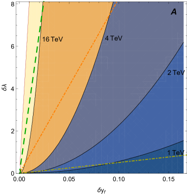
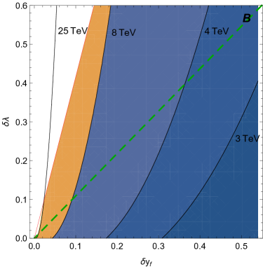
Figure 1: NP mass $M$ in dependence on the variation in the Yukawa couplings ($\delta y_{f}$) and in the triple-Higgs self coupling ($\delta\lambda$) in Scenario A (left) and B (right). The colored lines denote NP couplings of $g_{\ast}=1,4,8,4\pi$, respectively (from yellow to red). See text for details.

We now move to a numerical study of the sensitivities to NP masses ​$M$, considering (hypothetical) measurements of

1. a relative shift in yukawa couplings $\delta{y_{f}}$

2. the coefficient $C_{9}$ of the four-fermion operator ${\cal O}_{9}\equiv\frac{4G_{F}}{\sqrt{2}}V_{tb}V_{ts}^{\ast}\frac{\alpha}{4\pi}(\bar{s}_{L}\gamma_{\mu}b_{L})(\bar{\ell}\gamma^{\mu}\ell)$

3. a relative deviation in the Higgs self coupling $\delta\lambda$

4. the triple-gauge coupling (TGC) $\lambda_{Z}$.

These quantities are related to the coefficients of the operators in Table 3 as (see, e.g., deFlorian:2016spz )

$$\begin{split}\delta{y_{f}}&=v^{3}/(\sqrt{2}m_{f})\ c_{y_{f}}\\ C_{9}&=\frac{\sqrt{2}\pi}{\alpha\,G_{F}V_{tb}V_{ts}^{\ast}}\ c_{\text{\tiny$s_{L}\!b_{L}\!\ell\ell$}}\\ \delta\lambda&=2v^{4}/m_{h}^{2}\ c_{6}\\ \lambda_{Z}&=-6g^{2}\ c_{3W}\,.\end{split}$$ (5)

In that context, recall that $c_{\text{\tiny$s_{L}\!b_{L}\!\ell\ell$}}$ is assumed to scale like $V_{tb}V_{ts}^{\ast}g_{\ast}^{2}$, respecting MFV (such a structure is viable to allow for considerable effects in $C_{9}$, without being directly excluded from other measurements in flavor physics). A similar scaling holds in the case of partial compositeness, with the left-handed ($b$) quarks and leptons coupled significantly to the composite sector Megias:2016bde .

The expected sensitivities at the end of the high luminosity LHC (HL-LHC) run are $\delta{y_{f}}\sim 5\%$, for $f=(t),b,\tau$ (see, e.g., Peskin:2013xra ), $\delta\lambda\sim(20-30)\%$ Goertz:2013kp ; Goertz:2014qta ; Azatov:2015oxa , and $\lambda_{Z}\sim 10^{-3}$ Bian:2015zha , which will set the ballpark for the hypothetical measurements considered below. These values could still be improved, for example by the ILC, which could allow for $\delta{y_{f}}\sim 1\%$, for $f=b,c,\tau$ Peskin:2013xra , $\delta\lambda\sim 10\%$ Asner:2013psa , and $\lambda_{Z}\sim 10^{-4}$ Bian:2015zha . For $C_{9}$, on the other hand, we consider a value of $C_{9}\sim-1$, as suggested by experimental anomalies in $B$ physics, see footnote 9.

In Figs. 1-5, we finally explore the predictions for these quantities, induced by non-zero values of the corresponding coefficients, both for Scenario A and B. Employing relations (4) and (5), we can draw iso-contours of constant $M$ (dividing regions of different color) in two-dimensional planes spanned by the different (pseudo-)observables, where we can determine the heavy mass $M$ via a combined measurement of the latter. With a slight abuse of notation, we plot the absolute values of the corresponding quantities, keeping in mind that the signs of the various coefficients might vary.

We start by studying the correlations between $\delta{y_{f}}$ and $\delta\lambda$, visualized in Figure 1. We also present, as colored lines, the values of the coupling $g_{\ast}$ scanning the planes, where the dot-dashed yellow and orange lines correspond to NP couplings of $g_{\ast}=1,4$, respectively. The green dashed line visualizes the boundary of $g_{\ast}=8$, beyond which perturbation theory becomes problematic, while the red line, corresponding to $g_{\ast}=4\pi$, signals the complete breakdown of perturbation theory. We thus do not draw the colored regions beyond this point.

Looking at the left panel of the figure, representing Scenario A, we find that the observation of a deviation in Yukawa couplings of

• $\delta y_{f}=15\%$ together with a change in the trilinear Higgs self coupling of $\delta\lambda\sim 8$ indicates NP at $M\approx 3$ TeV.

Observing on the other hand

• $\delta y_{f}=1\%$ and $\delta\lambda\sim 2.5$ leads to a prediction of $M\approx 20$ TeV,

and thus to an explicit sensitivity to the mass, where a new particle is expected, far beyond direct collider reach. The maximally reachable sensitivity (respecting $g_{\ast}<8$ and experimental prospects) appears for $\delta y_{f}=1\%$, $\delta\lambda\sim 3$ and correspond to $M\approx 25$ TeV. The corresponding values for all pairs of pseudo-observables for the scenarios at hand will be summarized in Table 4.

Finally, the analysis leads to the further interesting observation that an effect of, say, $\sim 20\%$ in Yukawa couplings requires in fact sizable deviations in the self coupling of $\sim 250\%$, if no new physics resides below $1$ TeV. Similarly

• $\delta y_{f}=40\%$ would require a factor of almost $10$ in the self coupling, within LHC reach in the near future.

Thus, if such a deviation in yukawa couplings would be observed, while the self coupling would be constrained to $\delta\lambda<10$ (and no new physics would appear below a TeV), the large class of NP described by Scenario A could be basically excluded. Indeed, for constant $y_{f}$,

• increasing $\delta\lambda$ leads to larger NP masses,

which is due to the peculiar scaling of $\delta\lambda$ with a large power of $g_{\ast}$. In that context, the figure finally demonstrates that sizable deviations in the Higgs trilinear self coupling are possible, with small deviations elsewhere and a theory respecting perturbativity, as can be seen from the fact that a factor of a few in the former coupling is consistent with deviations in Yukawa interactions at/below the per cent level and moderate coupling strength ($g_{\ast}\ll 4\pi$), as well as large NP masses ($M>10$ TeV).

The situation is quite different in the SILH-like Scenario B, where perturbativity significantly limits the size of $\delta\lambda$ for moderate values of $\delta y_{f}$. A $10\%$ deviation in Yukawa couplings allows at most for a similar effect in the trilinear coupling, since larger values correspond to couplings $g_{\ast}$ entering a terrain where perturbation theory starts to become unreliable, as depicted by the dashed green line. Measuring, on the other hand, simultaneously such deviations,

• $\delta y_{f}=\delta\lambda=0.1$, leads to the knowledge that NP should show up at $M\approx 8\,$TeV,

assuming Scenario B. Moreover, seeing

• $\delta y_{f}$ approaching $\sim\!0.5$ and at most $\delta\lambda\lesssim 0.3$ requires NP appearing below $M\lesssim 3$ TeV

(without very weak couplings, since the orange dot-dashed line, signaling $g_{\ast}\leq 4$, does not yet appear) - otherwise the SILH is not realized in nature.

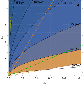
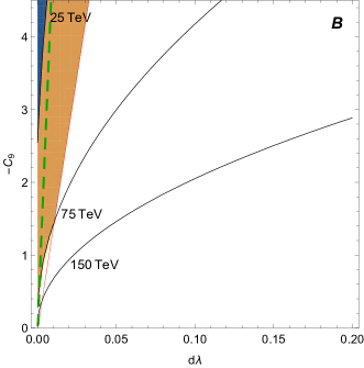
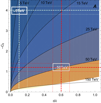
Figure 2: NP mass $M$ in dependence on the variation in the triple-Higgs self coupling ($\delta\lambda$) and the coefficient of the four fermion operator ${\cal O}_{9}$ ($C_{9}$) in Scenario A (upper panel, left) and B (upper panel, right). The colored lines denote NP couplings of $g_{\ast}=1,4,8,4\pi$, respectively (from yellow to red). The lower panel includes two hypothetical measurements of a signal in the $\lambda_{Z}-c_{9}$ plane and illustrates the correspondingly extracted masses of new particles in Scenario A. See text for details.

We now move to Figure 2, where we display the correlation between effects in the four-fermion operator ${\cal O}_{9}$ and $\delta\lambda$. Beginning again with Scenario A, shown in the upper left panel, we observe a potential sensitivity to very large NP masses, reaching even the $100$ TeV range. As discussed before, in this case there are actual experimental hints for a non-vanishing NP effect, corresponding to $C_{9}\sim-1$, which we depict by the red dashed line. Motivated by this anomaly, we now exemplify in the lower panel of the Figure in more detail a potential determination of the NP mass $M$. Assume that in fact a value of $C_{9}=-1.2\pm 0.2$ is established in the future Altmannshofer:2017fio , while the trilinear Higgs self-coupling exhibits a $\delta\lambda=(60\pm 10)\%$ correction. Given this information, we could conclude that $M\in\{40,60\}\,$TeV, which is derived from building the minimum and the maximum of $M$ over the four corners of the gray box denoted by $\sim 50$ TeV. On the contrary, a hypothetical value of $C_{9}=-4\pm 0.2$, together with the constraint $\delta\lambda\lesssim 10\%$ would lead to the prediction $M\lesssim 6$ TeV, if the underlying framework is Scenario A. The plot in the upper right panel summarizes the results in Scenario B. Here, this pair of observables is less rich, since moderate values of $C_{9}$ allow at most for $\delta\lambda\lesssim 3\,\%$, beyond any hope for detectability with current or planned experiments. Still, establishing any deviation in the triple Higgs coupling (without an excessive $C_{9}$) would again exclude the underlying SILH hypothesis.

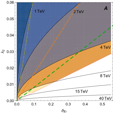
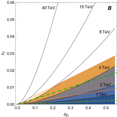
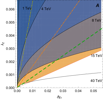
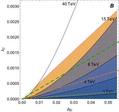
Figure 3: NP mass $M$ in dependence on the variation in the Yukawa couplings ($\delta y_{f}$) and the triple-gauge coupling ($\lambda_{Z}$) in Scenario A (left) and B (right). The colored lines denote NP couplings of $g_{\ast}=1,4,8,4\pi$, respectively (from yellow to red), and the lower panel shows a zoom into the plots of the upper panel. See text for details.

Next, we consider a simultaneous measurement of the TGC parameter $\lambda_{Z}$ and $\delta y_{f}$ in Scenario A. Here, a pretty strong constraint/exact measurement of a potential deviation in $\lambda_{Z}$ is necessary, together with non-vanishing effects in $\delta y_{f}$, approaching the perturbativity bound, in order to reach high masses. For example, $\lambda_{Z}\lesssim 1.5\,\%$ and $\delta y_{f}\sim 20\,\%$ leads to $M\approx 5\,$TeV, as can be read off from the upper left panel of Figure 3, while $\lambda_{Z}\lesssim 10^{-3}$ and $\delta y_{f}\sim 1\,\%$ leads to $M\approx 20\,$TeV, as is visible from the zoom into the small $\lambda_{Z}$ region in the lower left panel. In Scenario B, the scaling of $M$ with $\lambda_{Z}$ is inverted, due to the additional loop factor entering $c_{3V}$. While a $\delta y_{f}=5\,\%$ deviation in Yukawa couplings together with a $\lambda_{Z}=5\times 10^{-4}$ effect features $M\approx 3\,$TeV, the same deviation coming with $\lambda_{Z}=1.5\times 10^{-3}$ leads to $M\approx 10\,$TeV. Large effects in $\lambda_{Z}$ together with small $\delta y_{f}$, such as $\lambda_{Z}\gtrsim 1\,\%$ and $\delta y_{f}\lesssim 30\,\%$ are not possible in the perturbative regime, while the inverted case of $\lambda_{Z}\lesssim 2\times 10^{-3}$ and $\delta y_{f}\gtrsim 30\,\%$ is in conflict with the non-observation of new sub-TeV particles. In fact, sizable effects in one of the pseudo-observables require also non-negligible effects in the other. The same tendency holds also in Scenario A. In summary, while for the pair of $(\lambda_{Z},\delta y_{f})$ the potential to determine large NP masses is not tremendous, the strong correlations offer a valuable means to test/rule out the SILH or ALH paradigms. Moreover, the observation that the sensitivity to heavy masses increases if the coefficient that features the smaller power of $g_{\ast}$ becomes stronger constrained (which is $\lambda_{Z}$ ($\delta y_{f}$) in Scenario A (B)) is nicely confirmed in the plots.

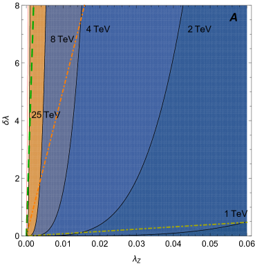
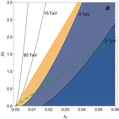
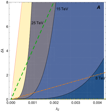
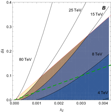
Figure 4: NP mass $M$ in dependence on the the triple-gauge coupling ($\lambda_{Z}$) and the variation in the triple-Higgs self coupling ($\delta\lambda$) in Scenario A (left) and B (right). The colored lines denote NP couplings of $g_{\ast}=1,4,8,4\pi$, respectively (from yellow to red), and the lower panel shows a zoom into the plots of the upper panel. See text for details.

Another interesting pair of (pseudo-)observables is $\delta\lambda$ and $\lambda_{Z}$, explored in Figure 4. In Scenario A, given in the left panel of the figure, large corrections to the trilinear Higgs self coupling are viable, with no measurable impact on $\lambda_{Z}$. Observing for example a $\delta\lambda=100\,\%$ correction simultaneously with $\lambda_{Z}=2\times 10^{-4}$ is consistent with the framework and corresponds to a very large NP mass of $M=50\,$TeV! Similarly, $\lambda_{Z}=2\times 10^{-3}$ allows for $\delta\lambda=8$ $-$ a measurement which would indicate that $M\approx 15\,$TeV. In Setup B, on the other hand, $\delta\lambda=100\,\%$ requires $\lambda_{Z}\gtrsim 3\,\%$ (see right panel of the figure), which is already in tension with current limits. NP masses corresponding to combined experimental results in this plane within collider reach are rather low, not exceeding $M\approx 8\,$TeV, which is reached for $\delta\lambda=10\,\%$ and $\lambda_{Z}=3\times 10^{-3}$.

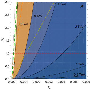
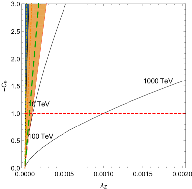
Figure 5: NP mass $M$ in dependence on the triple-gauge coupling ($\lambda_{Z}$) and the coefficient of the four fermion operator ${\cal O}_{9}$ ($C_{9}$) in Scenario A (left) and B (right). The colored lines denote NP couplings of $g_{\ast}=1,4,8,4\pi$, respectively (from yellow to red), and the horizontal dashed line depicts the currently preferred value of $C_{9}\sim-1$. See text for details.

The remaining plane to be discussed is spanned by $C_{9}$ and $\lambda_{Z}$. Here we can focus on Scenario A, depicted in the left panel of Figure 5, since measurable effects in Scenario B (in $\lambda_{Z}$), explored in the right panel of the same figure, are basically excluded from perturbativity. In the former setup, however, largely different NP masses can be discriminated. While $\lambda_{Z}=0.4\,\%$ with $C_{9}=-1$ leads to the prediction $M\approx 2\,$TeV, just at the boundary of the current direct reach, extracting $\lambda_{Z}=0.1\,\%$ and $C_{9}=-1.5$ induces $M\approx 10\,$TeV, and $\lambda_{Z}=3\times 10^{-4}$ with the same value for $C_{9}$ allows the conclusion that $M\approx 35\,$ TeV. At the same time, Scenario B strictly predicts a very small $\lambda_{Z}\sim{\cal O}(10^{-4})$, given a moderate $C_{9}$ not exceeding ${\cal O}(1)$. While for $\lambda_{Z}=10^{-4}$ and $C_{9}=-1.5$ one finds $M\approx 50\,$TeV, a sizable $\lambda_{Z}$ basically excludes this scenario.

Before concluding we will finally discuss the procedure lined out below eq. (4) for two simple explicit examples. To this end, consider first a measurement of $\lambda_{Z}\approx 0.15\,\%$ and $\delta\lambda\approx 10\,\%$. Employing Figure 4 (or eq. (4)), we deduce $M\approx 18\,$TeV for Scenario B and $M\approx 9\,$TeV for Scenario A, with couplings $g_{\ast}\approx 10$ and $g_{\ast}\approx 2$, respectively. With this information, we derive via eqs. (3) and (4) $\delta y_{f}\approx 3\,\%$ with $C_{9}\approx-18$ in Scenario B, while in Scenario A we obtain $\delta y_{f}\approx 0.5\,\%$ and $C_{9}\approx-2$. While Scenario B is clearly excluded, establishing a $C_{9}\lesssim-(1-2)$ would lead to a consistent picture of effects in Scenario A. Thus, given that nature respects approximately the scaling lined out in Table 3, we could conclude that NP is present at $M\approx 10\,$TeV, with a moderate coupling strength $g_{\ast}\approx 2$, in the reach of a future collider.

Clearly, less involved examples exist, where directly one of the two orthogonal scenarios is excluded. Consider thus finally $\delta\lambda=70\,\%$ and $C_{9}=-1.2$. From Figure 2 we can directly exclude Scenario B. For Scenario A, on the other hand, we derive $M\approx 50\,$TeV and $g_{\ast}\approx 8$. This leads now to the predictions $\delta y_{f}\approx 0.2\,\%$ and $\lambda_{Z}\approx 2\times 10^{-4}$, obviously in agreement with current limits, such that we obtain a consistent picture of rather strongly coupled NP significantly above energies testable at (near) future colliders.

We conclude this section noting that in less simple concrete models the final Wilson coefficients might deviate by a numerical ${\cal O}(1)$ factor from the above estimates - however, given that the scenario is broadly characterized by a single relevant NP coupling strength and a single mass scales (and not conflicting the broad assumptions we detailed), the NP mass that the analysis at hand will point to stays in the same ballpark and general correlations and tendencies remain valid.

4 Conclusions

We have shown how simultaneous measurements of (pseudo-)observables allow to determine explicitly the mass of NP particles, beyond direct reach. This is achieved by exploiting their different scaling with the NP coupling $g_{\ast}$, as derived after restoring the $\hbar$ dimensions of the operators, with the details of the procedure worked out in the body of the paper.

To summarize the results from the perspective of expected effects in the two orthogonal scenarios considered, in the ALH-like Scenario A ${\cal O}(1)$ effects are possible in $\delta\lambda$, without other problematic contributions, while sizable $\delta y_{f}$ of $\gtrsim 10\,\%$ require a large $\lambda_{Z}\gtrsim 1\,\%$ and a $C_{9}$ exceeding significantly experimental limits (under the given flavor hypothesis). Even a $\delta y_{f}\gtrsim 1\,\%$ leads to $\lambda_{Z}\gtrsim 0.1\,\%$ and $|C_{9}|\gtrsim 5$. In turn, sizable $C_{9}$ are possible without inducing large corrections to other pseudo-observables. Finally, a large $\lambda_{Z}$ at the per cent level induces also a detectable $\delta y_{f}$, unless the mass of the new physics is very low ($M\lesssim 1$ TeV), along with $|C_{9}|\gtrsim{\cal O}(1)$, while $\delta\lambda$ can easily remain at an unobservable level.

On the other hand, the SILH-like Scenario B predicts basically tiny $\delta\lambda$ and $\lambda_{Z}$, below a detectable level, since otherwise $|C_{9}|$ becomes too large (requiring perturbativity). Even ignoring the flavor-structure related $C_{9}$, sizable $\delta\lambda$ and $\lambda_{Z}$ at a level detectable in the near future are disfavored, since they also induce large corrections in Yukawa couplings around the current experimental sensitivity. Finding however a sizable $\delta y_{f}\sim 25\%$ would in turn lead unavoidably to a $\lambda_{Z}$ observable in the long-term LHC run (requiring $M\gtrsim 1\,$ TeV) and to a $C_{9}$ vastly exceeding limits. The strong and correlated predictions in this scenario offer a powerful means to test it indirectly in the near future with simple observations. Finally, sizable $C_{9}$ are viable in Scenario B, without any other observable prediction. The $(\delta\lambda,C_{9})$ plane is particularly promising for testing large $M$ in Scenario A, while in Scenario B the same holds true for $(\lambda_{Z},C_{9})$ and the figures can also be used to estimate if NP is expected to be detected first directly or indirectly.

The presented approach allows to test simple NP frameworks, such as the SILH or ALH, and to arrive at a mass $M$, as a (unique) solution to the experimental picture. While the article lines out the general procedure, in the presence of a signal dedicated studies along the lines worked out above will be in order to finally unveil the nature of the NP. After all, this work provides on overview of which patterns of NP can be expected and how an indication for the NP mass can be obtained, given only indirect observation, which can help to find the UV completion of the SM and to develop strategies to detect the NP directly.

A	$\delta{y_{f}}$	$\delta\lambda$	$\lambda_{Z}$	$c_{9}$
$\delta{y_{f}}$	-	25 TeV	25 TeV	-
$\delta\lambda$	25 TeV	-	70 TeV	150 TeV
$\lambda_{Z}$	25 TeV	70 TeV	-	70 TeV
$C_{9}$	-	150 TeV	70 TeV	-

B	$\delta{y_{f}}$	$\delta\lambda$	$\lambda_{Z}$	$c_{9}$
$\delta{y_{f}}$	-	8 TeV	25 TeV	-
$\delta\lambda$	8 TeV	-	8 TeV	N/A
$\lambda_{Z}$	25 TeV	8 TeV	-	40 TeV
$C_{9}$	-	N/A	40 TeV	-

Table 4: Maximal mass $M$ detectable, for each pair of pseudo-observables, considering ILC projections, see text for details.

References

- (1) W. Buchmuller and D. Wyler, “Effective Lagrangian Analysis of New Interactions and Flavor Conservation,” Nucl. Phys. B 268 (1986) 621.
- (2) K. Hagiwara, S. Ishihara, R. Szalapski and D. Zeppenfeld, “Low-energy effects of new interactions in the electroweak boson sector,” Phys. Rev. D 48 (1993) 2182.
- (3) B. Grzadkowski, M. Iskrzynski, M. Misiak and J. Rosiek, “Dimension-Six Terms in the Standard Model Lagrangian,” JHEP 1010 (2010) 085 [arXiv:1008.4884 [hep-ph]].
- (4) S. Weinberg, “Dynamical approach to current algebra,” Phys. Rev. Lett. 18 (1967) 188.
- (5) S. Weinberg, “Nonlinear realizations of chiral symmetry,” Phys. Rev. 166 (1968) 1568.
- (6) S. R. Coleman, J. Wess and B. Zumino, “Structure of phenomenological Lagrangians. 1.,” Phys. Rev. 177 (1969) 2239.
- (7) C. G. Callan, Jr., S. R. Coleman, J. Wess and B. Zumino, “Structure of phenomenological Lagrangians. 2.,” Phys. Rev. 177 (1969) 2247.
- (8) R. F. Dashen, “Chiral SU(3) x SU(3) as a symmetry of the strong interactions,” Phys. Rev. 183 (1969) 1245.
- (9) R. F. Dashen and M. Weinstein, “Soft pions, chiral symmetry, and phenomenological lagrangians,” Phys. Rev. 183 (1969) 1261.
- (10) L. F. Li and H. Pagels, “Perturbation theory about a Goldstone symmetry,” Phys. Rev. Lett. 26 (1971) 1204.
- (11) K. G. Wilson, “Renormalization group and critical phenomena. 1. Renormalization group and the Kadanoff scaling picture, 2. Phase space cell analysis of critical behavior,” Phys. Rev. B 4 (1971) 3174, 3184.
- (12) K. G. Wilson and J. B. Kogut, “The Renormalization group and the epsilon expansion,” Phys. Rept. 12 (1974) 75.
- (13) T. Appelquist and J. Carazzone, “Infrared Singularities and Massive Fields,” Phys. Rev. D 11 (1975) 2856.
- (14) S. Weinberg, “Phenomenological Lagrangians,” Physica A 96 (1979) 327.
- (15) S. Weinberg, “Baryon and Lepton Nonconserving Processes,” Phys. Rev. Lett. 43 (1979) 1566.
- (16) F. Wilczek and A. Zee, “Operator Analysis of Nucleon Decay,” Phys. Rev. Lett. 43 (1979) 1571.
- (17) S. Weinberg, “Effective Gauge Theories,” Phys. Lett. 91B (1980) 51.
- (18) H. A. Weldon and A. Zee, “Operator Analysis of New Physics,” Nucl. Phys. B 173 (1980) 269.
- (19) J. Polchinski, “Effective field theory and the Fermi surface,” In *Boulder 1992, Proceedings, Recent directions in particle theory* 235-274, and Calif. Univ. Santa Barbara - NSF-ITP-92-132 (92,rec.Nov.) 39 p. (220633) Texas Univ. Austin - UTTG-92-20 (92,rec.Nov.) 39 p [hep-th/9210046].
- (20) H. Georgi, “Effective field theory,” Ann. Rev. Nucl. Part. Sci. 43 (1993) 209.
- (21) A. Pich, “Effective field theory: Course,” hep-ph/9806303.
- (22) A. J. Buras, “Weak Hamiltonian, CP violation and rare decays,” hep-ph/9806471.
- (23) M. Neubert, “Effective field theory and heavy quark physics,” hep-ph/0512222.
- (24) C. P. Burgess, “Introduction to Effective Field Theory,” Ann. Rev. Nucl. Part. Sci. 57 (2007) 329 [hep-th/0701053].
- (25) A. Falkowski, “Effective field theory approach to LHC Higgs data,” Pramana 87 (2016) no.3, 39 [arXiv:1505.00046 [hep-ph]].
- (26) D. de Florian et al. [LHC Higgs Cross Section Working Group], “Handbook of LHC Higgs Cross Sections: 4. Deciphering the Nature of the Higgs Sector,” arXiv:1610.07922 [hep-ph].
- (27) G. F. Giudice and M. McCullough, “A Clockwork Theory,” JHEP 1702 (2017) 036 [arXiv:1610.07962 [hep-ph]].
- (28) G. F. Giudice, C. Grojean, A. Pomarol and R. Rattazzi, “The Strongly-Interacting Light Higgs,” JHEP 0706 (2007) 045 [hep-ph/0703164].
- (29) M. A. Luty, “Naive dimensional analysis and supersymmetry,” Phys. Rev. D 57 (1998) 1531 [hep-ph/9706235].
- (30) A. G. Cohen, D. B. Kaplan and A. E. Nelson, “Counting 4 pis in strongly coupled supersymmetry,” Phys. Lett. B 412 (1997) 301 [hep-ph/9706275].
- (31) R. Contino, A. Falkowski, F. Goertz, C. Grojean and F. Riva, “On the Validity of the Effective Field Theory Approach to SM Precision Tests,” JHEP 1607 (2016) 144 [arXiv:1604.06444 [hep-ph]].
- (32) K. Agashe, R. Contino and A. Pomarol, “The Minimal composite Higgs model,” Nucl. Phys. B 719 (2005) 165 [hep-ph/0412089].
- (33) D. Liu, A. Pomarol, R. Rattazzi and F. Riva, “Patterns of Strong Coupling for LHC Searches,” JHEP 1611 (2016) 141 [arXiv:1603.03064 [hep-ph]].
- (34) J. de Blas, M. Chala, M. Perez-Victoria and J. Santiago, “Observable Effects of General New Scalar Particles,” JHEP 1504 (2015) 078 [arXiv:1412.8480 [hep-ph]].
- (35) B. Henning, X. Lu and H. Murayama, “How to use the Standard Model effective field theory,” JHEP 1601 (2016) 023 [arXiv:1412.1837 [hep-ph]].
- (36) G. D’Ambrosio, G. F. Giudice, G. Isidori and A. Strumia, “Minimal flavor violation: An Effective field theory approach,” Nucl. Phys. B 645 (2002) 155 [hep-ph/0207036].
- (37) S. Descotes-Genon, J. Matias and J. Virto, “Understanding the Anomaly,” Phys. Rev. D 88 (2013) 074002 [arXiv:1307.5683 [hep-ph]].
- (38) R. Gauld, F. Goertz and U. Haisch, “On minimal explanations of the anomaly,” Phys. Rev. D 89 (2014) 015005 [arXiv:1308.1959 [hep-ph]].
- (39) W. Altmannshofer, C. Niehoff, P. Stangl and D. M. Straub, “Status of the anomaly after Moriond 2017,” Eur. Phys. J. C 77 (2017) no.6, 377 [arXiv:1703.09189 [hep-ph]].
- (40) G. D’Amico, M. Nardecchia, P. Panci, F. Sannino, A. Strumia, R. Torre and A. Urbano, “Flavour anomalies after the measurement,” arXiv:1704.05438 [hep-ph].
- (41) E. Megias, G. Panico, O. Pujolas and M. Quiros, JHEP 1609 (2016) 118 doi:10.1007/JHEP09(2016)118 [arXiv:1608.02362 [hep-ph]].
- (42) M. E. Peskin, “Estimation of LHC and ILC Capabilities for Precision Higgs Boson Coupling Measurements,” arXiv:1312.4974 [hep-ph].
- (43) F. Goertz, A. Papaefstathiou, L. L. Yang and J. Zurita, “Higgs Boson self-coupling measurements using ratios of cross sections,” JHEP 1306 (2013) 016 [arXiv:1301.3492 [hep-ph]].
- (44) F. Goertz, A. Papaefstathiou, L. L. Yang and J. Zurita, “Higgs boson pair production in the D=6 extension of the SM,” JHEP 1504 (2015) 167 [arXiv:1410.3471 [hep-ph]].
- (45) A. Azatov, R. Contino, G. Panico and M. Son, “Effective field theory analysis of double Higgs boson production via gluon fusion,” Phys. Rev. D 92 (2015) no.3, 035001 [arXiv:1502.00539 [hep-ph]].
- (46) L. Bian, J. Shu and Y. Zhang, “Prospects for Triple Gauge Coupling Measurements at Future Lepton Colliders and the 14 TeV LHC,” JHEP 1509 (2015) 206 [arXiv:1507.02238 [hep-ph]].
- (47) D. M. Asner et al., “ILC Higgs White Paper,” arXiv:1310.0763 [hep-ph].