MarrNet: 3D Shape Reconstruction via 2.5D Sketches

Abstract

3D object reconstruction from a single image is a highly under-determined problem, requiring strong prior knowledge of plausible 3D shapes. This introduces challenges for learning-based approaches, as 3D object annotations are scarce in real images. Previous work chose to train on synthetic data with ground truth 3D information, but suffered from domain adaptation when tested on real data.

In this work, we propose MarrNet, an end-to-end trainable model that sequentially estimates 2.5D sketches and 3D object shape. Our disentangled, two-step formulation has three advantages. First, compared to full 3D shape, 2.5D sketches are much easier to be recovered from a 2D image; models that recover 2.5D sketches are also more likely to transfer from synthetic to real data. Second, for 3D reconstruction from 2.5D sketches, systems can learn purely from synthetic data. This is because we can easily render realistic 2.5D sketches without modeling object appearance variations in real images, including lighting, texture, etc. This further relieves the domain adaptation problem. Third, we derive differentiable projective functions from 3D shape to 2.5D sketches; the framework is therefore end-to-end trainable on real images, requiring no human annotations. Our model achieves state-of-the-art performance on 3D shape reconstruction.

1 Introduction

Humans quickly recognize 3D shapes from a single image. Figure 1a shows a number of images of chairs; despite their drastic difference in object texture, material, environment lighting, and background, humans easily recognize they have very similar 3D shapes. What is the most essential information that makes this happen?

Researchers in human perception argued that our 3D perception could rely on recovering 2.5D sketches (Marr, 1982), which include intrinsic images (Barrow and Tenenbaum, 1978; Tappen et al., 2003) like depth and surface normal maps (Figure 1b). Intrinsic images disentangle object appearance variations in texture, albedo, lighting, etc., with its shape, which retains all information from the observed image for 3D reconstruction. Humans further combine 2.5D sketches and a shape prior learned from past experience to reconstruct a full 3D shape (Figure 1c). In the field of computer vision, there have also been abundant works exploiting the idea for reconstruction 3D shapes of faces (Kemelmacher-Shlizerman and Basri, 2011), objects (Tappen et al., 2003), and scenes (Hoiem et al., 2005; Saxena et al., 2009).

Recently, researchers attempted to tackle the problem of single image 3D reconstruction with deep learning. These approaches usually regress a 3D shape from a single RGB image directly (Tulsiani et al., 2017; Choy et al., 2016; Wu et al., 2016b). In contrast, we propose a two-step while end-to-end trainable pipeline, sequentially recovering 2.5D sketches (depth and normal maps) and a 3D shape. We use an encoder-decoder structure for each component of the framework, and also enforce the reprojection consistency between the estimated sketch and the 3D shape. We name it MarrNet, for its close resemblance to David Marr’s theory of perception (Marr, 1982).

Our approach offers several unique advantages. First, the use of 2.5D sketches releases the burden on domain transfer. As single image 3D reconstruction is a highly under-constrained problem, strong prior knowledge of object shapes is needed. This poses challenges to learning-based methods, as accurate 3D object annotations in real images are rare. Most previous methods turned to training purely on synthetic data (Tulsiani et al., 2017; Choy et al., 2016; Girdhar et al., 2016). However, these approaches often suffer from the domain adaption issue due to imperfect rendering. Learning 2.5D sketches from images, in comparison, is much easier and more robust to transfer from synthetic to real images, as shown in Section 4.

Further, as our second step recovers 3D shape from 2.5D sketches — an abstraction of the raw input image, it can be trained purely relying on synthetic data. Though rendering diverse realistic images is challenging, it is straightforward to obtain almost perfect object surface normals and depths from a graphics engine. This further relieves the domain adaptation issue.

We also enforce differentiable constraints between 2.5D sketches and 3D shape, making our system end-to-end trainable, even on real images without any annotations. Given a set of unlabeled images, our algorithm, pre-trained on synthetic data, can infer the 2.5D sketches of objects in the image, and use it to refine its estimation of objects’ 3D shape. This self-supervised feature enhances its performance on images from different domains.

We evaluate our framework on both synthetic images of objects from ShapeNet (Chang et al., 2015), and real images from the PASCAL 3D+ dataset (Xiang et al., 2014). We demonstrate that our framework performs well on 3D shape reconstruction, both qualitatively and quantitatively.

Our contributions are three-fold: inspired by visual cognition theory, we propose a two-step, disentangled formulation for single image 3D reconstruction via 2.5D sketches; we develop a novel, end-to-end trainable model with a differentiable projection layer that ensures consistency between 3D shape and mid-level representations; we demonstrate its effectiveness on 2.5D sketch transfer and 3D shape reconstruction on both synthetic and real data.

Figure 1: Objects in real images (a) are subject to appearance variations regarding color, texture, lighting, material, background, etc. Despite this, their 2.5D sketches like surface normal and depth maps remain constant (b). The 2.5D sketches can be seen as an abstraction of the image, retaining all information about the 3D shape of the object inside. We combine the sketches with learned shape priors to reconstruct the full 3D shape (c).

2 Related Work

2.5D Sketch Recovery

Estimating 2.5D sketches has been a long-standing problem in computer vision. In the past, researchers have explored recovering 2.5D shape from shading, texture, or color images (Horn and Brooks, 1989; Zhang et al., 1999; Tappen et al., 2003; Barron and Malik, 2015; Weiss, 2001; Bell et al., 2014). With the development of depth sensors (Izadi et al., 2011) and larger scale RGB-D datasets (Silberman et al., 2012; Song et al., 2017; McCormac et al., 2017), there have also been papers on estimating depth (Chen et al., 2016; Eigen and Fergus, 2015), surface normals (Bansal and Russell, 2016; Wang et al., 2015), and other intrinsic images (Shi et al., 2017; Janner et al., 2017) with deep networks. Our method employs 2.5D estimation as a component, but targets reconstructing full 3D shape of an object.

Single Image 3D Reconstruction

The problem of recovering object shape from a single image is challenging, as it requires both powerful recognition systems and prior shape knowledge. With the development of large-scale shape repository like ShapeNet (Chang et al., 2015), researchers developed models encoding shape prior for this task (Girdhar et al., 2016; Choy et al., 2016; Tulsiani et al., 2017; Wu et al., 2016b; Kar et al., 2015; Kanazawa et al., 2016; Soltani et al., 2017), with extension to scenes (Song et al., 2017). These methods typically regress a voxelized 3D shape directly from an input image, and rely on synthetic data or 2D masks for training. In comparison, our formulation tackles domain difference better, as it can be end-to-end fine-tuned on images without any annotations.

2D-3D Consistency

It is intuitive and practically helpful to constrain the reconstructed 3D shape to be consistent with 2D observations. Researchers have explored this idea for decades (Lowe, 1987). This idea is also widely used in 3D shape completion from depths or silhouettes (Firman et al., 2016; Rock et al., 2015; Dai et al., 2017). Recently, a few papers discussed enforcing differentiable 2D-3D constraints between shape and silhouettes, enabling joint training of deep networks for 3D reconstruction (Wu et al., 2016a; Yan et al., 2016; Rezende et al., 2016; Tulsiani et al., 2017). In our paper, we exploit this idea to develop differentiable constraints on the consistency between various 2.5D sketches and 3D shape.

3 Approach

Figure 2: Our model (MarrNet) has three major components: (a) 2.5D sketch estimation, (b) 3D shape estimation, and (c) a loss function for reprojection consistency. MarrNet first recovers object normal, depth, and silhouette images from an RGB image. It then regresses the 3D shape from the 2.5D sketches. In both steps, it uses an encoding-decoding network. It finally employs a reprojection consistency loss to ensure the estimated 3D shape aligns with the 2.5D sketches. The entire framework can be trained end-to-end.

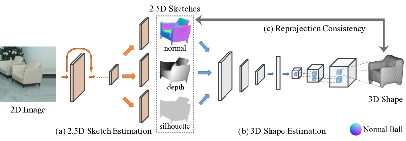
To recover the 3D structure from a single view RGB image, our MarrNet contains three parts: first, a 2.5D sketch estimator, which predicts the depth, surface normal, and silhouette images of the object (Figure 2a); second, a 3D shape estimator, which infers 3D object shape using a voxel representation (Figure 2b); third, a reprojection consistency function, enforcing the alignment between the estimated 3D structure and inferred 2.5D sketches (Figure 2c).

3.1 2.5D Sketch Estimation

The first component of our network (Figure 2a) takes a 2D RGB image as input, and predicts its 2.5D sketch: surface normal, depth, and silhouette. The goal of the 2.5D sketch estimation step is to distill intrinsic object properties from input images, while discarding properties that are non-essential for the task of 3D reconstruction, such as object texture and lighting.

We use an encoder-decoder network architecture for 2.5D sketch estimation. Our encoder is a ResNet-18 (He et al., 2015), encoding a 256$\times$256 RGB image into 512 feature maps of size 8$\times$8. The decoder contains four sets of 5$\times$5 fully convolutional and ReLU layers, followed by four sets of 1$\times$1 convolutional and ReLU layers. It outputs the corresponding depth, surface normal, and silhouette images, also at the resolution of 256$\times$256.

3.2 3D Shape Estimation

The second part of our framework (Figure 2b) infers 3D object shape from estimated 2.5D sketches. Here, the network focuses on learning the shape prior that explains input well. As it takes only surface normal and depth images as input, it can be trained on synthetic data, without suffering from the domain adaption problem: it is straightforward to render nearly perfect 2.5D sketches, but much harder to render realistic images.

The network architecture is inspired by the TL network (Girdhar et al., 2016), and the 3D-VAE-GAN (Wu et al., 2016b), again with an encoding-decoding style. It takes a normal image and a depth image as input (both masked by the estimated silhouette), maps them to a 200-dim vector via five sets of convolutional, ReLU, and pooling layers, followed by two fully connected layers. The detailed encoder structure can be found in Girdhar et al. (2016). The vector then goes through a decoder, which consists of five fully convolutional and ReLU layers to output a 128$\times$128$\times$128 voxel-based reconstruction of the input. The detailed encoder structure can be found in Wu et al. (2016b).

3.3 Reprojection Consistency

Figure 3: Reprojection consistency between 2.5D sketches and 3D shape. Left and middle: the criteria for depths and silhouettes; right: the criterion for surface normals. See Section 3.3 for details.

There have been works attempting to enforce the consistency between estimated 3D shape and 2D representations in a neural network (Yan et al., 2016; Rezende et al., 2016; Wu et al., 2016a; Tulsiani et al., 2017). Here, we explore novel ways to include a reprojection consistency loss between the predicted 3D shape and the estimated 2.5D sketch, consisting of a depth reprojection loss and a surface normal reprojection loss.

We use $v_{x,y,z}$ to represent the value at position $(x,y,z)$ in a 3D voxel grid, assuming that $v_{x,y,z}\in[0,1]$, $\forall x,y,z$. We use $d_{x,y}$ to denote the estimated depth at position $(x,y)$, and $n_{x,y}=(n_{a},n_{b},n_{c})$ to denote the estimated surface normal. We assume orthographic projection in this work.

Depths

The projected depth loss tries to guarantee that the voxel with depth $v_{x,y,d_{x,y}}$ should be 1, and all voxels in front of it should be $0$. This ensures the estimated 3D shape matches the estimated depth values.

As illustrated in Figure 3a, we define projected depth loss as follows:

$$L_{\text{depth}}(x,y,z)=\begin{cases}v^{2}_{x,y,z},&z<d_{x,y}\\ (1-v_{x,y,z})^{2},&z=d_{x,y}\\ 0,&z>d_{x,y}\\ \end{cases}.$$ (1)

The gradients are

$$\frac{\partial{L_{\text{depth}}(x,y,z)}}{\partial{v_{x,y,z}}}=\begin{cases}2v_{x,y,z},&z<d_{x,y}\\ 2(v_{x,y,z}-1),&z=d_{x,y}\\ 0,&z>d_{x,y}\\ \end{cases}.$$ (2)

When $d_{x,y}=\infty$, our depth criterion reduces to a special case — the silhouette criterion. As shown in Figure 3b, for a line that has no intersection with the shape, all voxels in it should be 0.

Surface normals

As vectors $n_{x}=(0,-n_{c},n_{b})$ and $n_{y}=(-n_{c},0,n_{a})$ are orthogonal to the normal vector $n_{x,y}=(n_{a},n_{b},n_{c})$, we can normalize them to obtain two vectors, $n_{x}^{\prime}=(0,-1,n_{b}/n_{c})$ and $n_{y}^{\prime}=(-1,0,n_{a}/n_{c})$, both on the estimated surface plane at $(x,y,z)$. The projected surface normal loss tries to guarantee that the voxels at $(x,y,z)\pm n_{x}^{\prime}$ and $(x,y,z)\pm n_{+y}$ should be 1 to match the estimated surface normals. These constraints only apply when the target voxels are inside the estimated silhouette.

As shown in Figure 3c, let $z=d_{x,y}$, the projected surface normal loss is defined as

$$L_{\text{normal}}(x,y,z)=\; \left(1-v_{x,y-1,z+\frac{n_{b}}{n_{c}}}\right)^{2}+\left(1-v_{x,y+1,z-\frac{n_{b}}{n_{c}}}\right)^{2}+$$

$$\left(1-v_{x-1,y,z+\frac{n_{a}}{n_{c}}}\right)^{2}+\left(1-v_{x+1,y,z-\frac{n_{a}}{n_{c}}}\right)^{2}.$$ (3)

Then the gradients along the $x$ direction are

$$\frac{\partial{L_{\text{normal}}(x,y,z)}}{\partial{v_{x-1,y,z+\frac{n_{a}}{n_{c}}}}}=2\left(v_{x-1,y,z+\frac{n_{a}}{n_{c}}}-1\right)\quad\text{and}\quad\frac{\partial{L_{\text{normal}}(x,y,z)}}{\partial{v_{x+1,y,z-\frac{n_{a}}{n_{c}}}}}=2\left(v_{x+1,y,z-\frac{n_{a}}{n_{c}}}-1\right).$$ (4)

The gradients along the $y$ direction are similar.

3.4 Training paradigm

We employ a two-step training paradigm. We first train the 2.5D sketch estimation and the 3D shape estimation components separately on synthetic images; we then fine-tune the network on real images.

For pre-training, we use synthetic images of ShapeNet objects. The 2.5D sketch estimator is trained using the ground truth surface normal, depth, and silhouette images with a L2 loss. The 3D interpreter is trained using ground truth voxels and a cross-entropy loss. Please see Section 4.1 for details on data preparation.

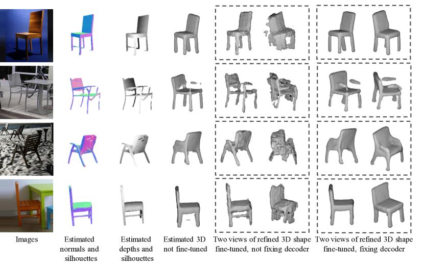
The reprojection consistency loss is used to fine-tune the 3D estimation component of our model on real images, using the predicted normal, depth, and silhouette. We observe that a straightforward implementation leads to shapes that explain 2.5D sketches well, but with unrealistic appearance. This is because the 3D estimation module overfits the images without preserving the learned 3D shape prior. See Figure 5 for examples, and Section 4.2 for more details.

We therefore choose to fix the decoder of the 3D estimator and only fine-tune the encoder. During testing, our method can be self-supervised, i.e., we can fine-tune even on a single image without any annotations. In practice, we fine-tune our model separately on each image for 40 iterations. For each test image, fine-tuning takes up to 10 seconds on a modern GPU; without fine-tuning, testing time is around 100 milliseconds. We use SGD for optimization with a batch size of 4, a learning rate of 0.001, and a momentum of 0.9. We implemented our framework in Torch7 (Collobert et al., 2011).

Figure 4: Results on rendered images of ShapeNet objects (Chang et al., 2015). From left to right: input, estimated normal map, estimated depth map, our prediction, a baseline algorithm that predicts 3D shape directly from RGB input without modeling 2.5D sketch, and ground truth. Both normal and depth maps are masked by predicted silhouettes. Our method is able to recover shapes with smoother surfaces and finer details.

Figure 5: We present an ablation study, where we compare variants of our models. From left to right: input, estimated normal, estimated depth, 3D prediction before fine-tuning, two views of the 3D prediction after fine-tuning without fixing decoder, and two views of the 3D prediction after fine-tuning with the decoder fixed. When the decoder is not fixed, the model explains the 2.5D sketch well, but fails to preserve the learned shape prior. Fine-tuning with a fixed decoder resolves the issue.

4 Evaluation

Figure 6: 3D reconstructions of chairs on the Pascal 3D+ (Xiang et al., 2014) dataset. From left to right: input, the ground truth shape from the dataset, 3D estimation by DRC (Tulsiani et al., 2017), and two views of MarrNet predictions. Our model recovers more accurate 3D shapes.

	DRC	MarrNet	GT
DRC	50	26	17
MarrNet	74	50	42
Ground truth	83	58	50

Table 1: Human preferences on chairs in PASCAL 3D+ (Xiang et al., 2014). We compare MarrNet with the state-of-the-art (DRC) (Tulsiani et al., 2017), and the ground truth provided by the dataset. Each number shows the percentage of humans prefer the left method to the top one. MarrNet is preferred 74% of the time to DRC, and 42% of the time to ground truth.

Figure 7: Failure cases on Pascal 3D+. Our algorithm does not perform well on recovering complex, thin structure, and sometimes fails when the estimated mask is very inaccurate.

Figure 8: 3D reconstruction of chairs on the IKEA (Lim et al., 2013) dataset. From left to right: input, ground truth, 3D estimation by 3D-VAE-GAN (Wu et al., 2016b), and two views of MarrNet predictions. Our modelrecovers more details compared to 3D-VAE-GAN.

Figure 9: 3D reconstructions of airplanes and cars from PASCAL 3D+. From left to right: input, the ground truth shape from the dataset, 3D estimation by DRC (Tulsiani et al., 2017), and two views of MarrNet predictions.

Figure 10: 3D reconstruction of objects from multiple categories on the PASCAL 3D+ (Xiang et al., 2014) dataset. Under this setup MarrNet also recovers 3D shape well.

In this section, we present both qualitative and quantitative results on single image 3D reconstruction using variants of our framework. We evaluate our entire framework on both synthetic and real-life images on three datasets.

4.1 3D Reconstruction on ShapeNet

Data

We start with experiments on synthesized images of ShapeNet chairs (Chang et al., 2015). We put objects in front of random backgrounds from the SUN database (Xiao et al., 2010), and render the corresponding RGB, depth, surface normal, and silhouette images. We use a physics-based renderer, Mitsuba (Jakob, 2010), to obtain more realistic images. For each of the 6,778 ShapeNet chairs, we render 20 images of random viewpoints.

Methods

We follow the training paradigm described in Section 3.4, but without the final fine-tuning stage, as ground truth 3D shapes are available on this synthetic dataset. Specifically, the 2.5D sketch estimator is trained using ground truth depth, normal and silhouette images and a L2 reconstruction loss. The 3D shape estimation module takes in the masked ground truth depth and normal images as input, and predicts 3D voxels of size 128$\times$128$\times$128 with a binary cross entropy loss.

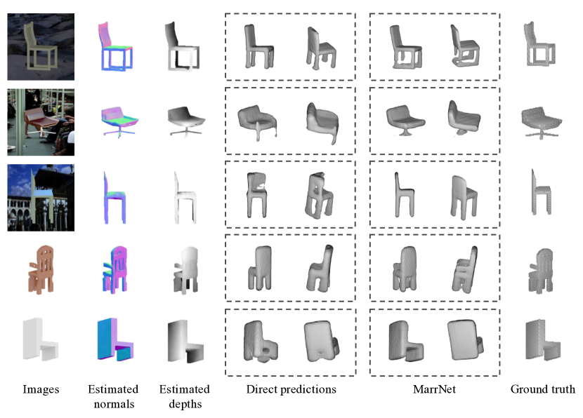
We compare MarrNet with a baseline that predicts 3D shape directly from an RGB image, without modeling 2.5D sketches. The baseline employs the same architecture as our 3D shape estimator (Section 3.2). We show qualitative results in Figure 4. Our estimated surface normal and depth images abstract out non-essential information like textures and lighting in the RGB image, while preserving intrinsic information about object shape. Compared with the direct prediction baseline, our model outputs objects with more details and smoother surfaces. For quantitative evaluation, previous works usually compute the Intersection-over-Union (IoU) (Tulsiani et al., 2017; Choy et al., 2016). Our full model achieves a higher IoU (0.57) than the direct prediction baseline (0.52).

4.2 3D Reconstruction on Pascal 3D+

Data

PASCAL 3D+ dataset (Xiang et al., 2014) provides (rough) 3D models for objects in real-life images. Here, we use the same test set of PASCAL 3D+ with earlier works (Tulsiani et al., 2017).

Methods

We follow the paradigm described in Section 3.4: we first train each module separately on the ShapeNet dataset, and then fine-tune them on the PASCAL 3D+ dataset. Unlike previous works (Tulsiani et al., 2017), our model requires no silhouettes as input during fine-tuning; it instead estimates silhouette jointly.

As an ablation study, we compare three variants of our model: first, the model trained using ShapeNet data only, without fine-tuning; second, the fine-tuned model whose decoder is not fixed during fine-tuning; and third, the full model whose decoder is fixed during fine-tuning. We also compare with the state-of-the-art method (DRC) (Tulsiani et al., 2017), and the provided ground truth shapes.

Results

The results of our ablation study are shown in Figure 5. The model trained on synthetic data provides a reasonable shape estimate. If we fine-tune the model on Pascal 3D+ without fixing the decoder, the output voxels explain the 2.5D sketch data well, but fail to preserve the learned shape prior, leading to impossible shapes from certain views. Our final model, fine-tuned with the decoder fixed, keeps the shape prior and provides more details of the shape.

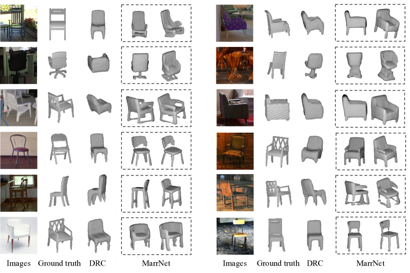
We show more results in Figure 6, where we compare with the state-of-the-art (DRC) (Tulsiani et al., 2017), and the provided ground truth shapes. Quantitatively, our algorithm achieves a higher IoU over these methods (MarrNet 0.39 vs. DRC 0.34). However, we find the IoU metric sub-optimal for three reasons. First, measuring 3D shape similarity is a challenging yet unsolved problem, and IoU prefers models that predict mean shapes consistently, with no emphasize on details. Second, as object shape can only be reconstructed up to scale from a single image, it requires searching over all possible scales during the computation of IoU, making it less efficient. Third, as discussed in Tulsiani et al. (2017), PASCAL 3D+ has only rough 3D annotations (10 CAD chair models for all images). Computing IoU with these shapes would thus not be the most informative evaluation metric.

We instead conduct human studies, where we show users the input image and two reconstructions, and ask them to choose the one that looks closer to the shape in the image. We show each test image to 10 human subjects. As shown in Table 1, our reconstruction is preferred 74% of the time to DRC, and 42% of the time to ground truth, showing a clear advantage.

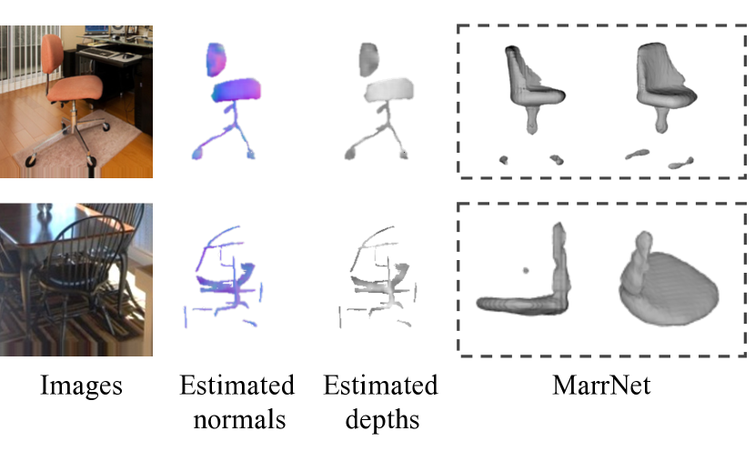
We present some failure cases in Figure 7. Our algorithm does not perform well on recovering complex, thin structure, and sometimes fails when the estimated mask is very inaccurate. Also, while DRC may benefit from multi-view supervision, we have only evaluated MarrNet given a single view of the shape, though adapting our formulation to multi-view data should be straightforward.

4.3 3D Reconstruction on IKEA

Data

The IKEA dataset (Lim et al., 2013) contains images of IKEA furniture, along with accurate 3D shape and pose annotations. These images are challenging, as objects are often heavily occluded or cropped. We also evaluate our model on the IKEA dataset.

Results

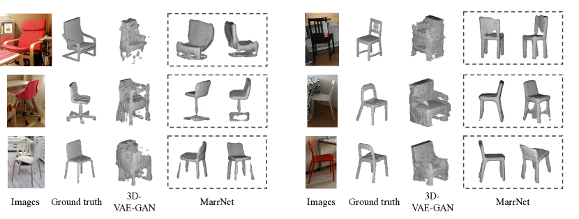
We show qualitative results in Figure 8, where we compare with estimations by 3D-VAE-GAN (Wu et al., 2016b) and the ground truth. As shown in the figure, our model can deal with mild occlusions in real life scenarios. We also conduct human studies on the IKEA dataset. Results show that 61% of the subjects prefer our reconstructions to those of 3D-VAE-GAN.

4.4 Extensions

We also apply our framework on cars and airplanes. We use the same setup as that for chairs. As shown in Figure 9, shape details like the horizontal stabilizer and rear-view mirrors are recovered by our model. We further train MarrNet jointly on all three object categories, and show results in Figure 10. Our model successfully recovers shapes of different categories.

5 Conclusion

We proposed MarrNet, a novel model that explicitly models 2.5D sketches for single image 3D shape reconstruction. The use of 2.5D sketches enhanced the model’s performance, and made it easily adaptive to images across domains or even categories. We also developed differentiable loss functions for the consistency between 3D shape and 2.5D sketches, so that MarrNet can be end-to-end fine-tuned on real images without annotations. Experiments demonstrated that our model performs well, and is preferred by human annotators over competitors.

Acknowledgements

We thank Shubham Tulsiani for sharing the DRC results, and Chengkai Zhang for the help on shape visualization. This work is supported by NSF #1212849 and #1447476, ONR MURI N00014-16-1-2007, the Center for Brain, Minds and Machines (NSF #1231216), Toyota Research Institute, Samsung, and Shell.

References

- Bansal and Russell [2016] Aayush Bansal and Bryan Russell. Marr revisited: 2d-3d alignment via surface normal prediction. In CVPR, 2016.
- Barron and Malik [2015] Jonathan T Barron and Jitendra Malik. Shape, illumination, and reflectance from shading. IEEE TPAMI, 37(8):1670–1687, 2015.
- Barrow and Tenenbaum [1978] Harry G Barrow and Jay M Tenenbaum. Recovering intrinsic scene characteristics from images. Computer vision systems, 1978.
- Bell et al. [2014] Sean Bell, Kavita Bala, and Noah Snavely. Intrinsic images in the wild. ACM TOG, 33(4):159, 2014.
- Chang et al. [2015] Angel X Chang, Thomas Funkhouser, Leonidas Guibas, Pat Hanrahan, Qixing Huang, Zimo Li, Silvio Savarese, Manolis Savva, Shuran Song, Hao Su, et al. Shapenet: An information-rich 3d model repository. arXiv:1512.03012, 2015.
- Chen et al. [2016] Weifeng Chen, Zhao Fu, Dawei Yang, and Jia Deng. Single-image depth perception in the wild. In NIPS, 2016.
- Choy et al. [2016] Christopher B Choy, Danfei Xu, JunYoung Gwak, Kevin Chen, and Silvio Savarese. 3d-r2n2: A unified approach for single and multi-view 3d object reconstruction. In ECCV, 2016.
- Collobert et al. [2011] Ronan Collobert, Koray Kavukcuoglu, and Clément Farabet. Torch7: A matlab-like environment for machine learning. In BigLearn, NIPS Workshop, 2011.
- Dai et al. [2017] Angela Dai, Charles Ruizhongtai Qi, and Matthias Nießner. Shape completion using 3d-encoder-predictor cnns and shape synthesis. In CVPR, 2017.
- Eigen and Fergus [2015] David Eigen and Rob Fergus. Predicting depth, surface normals and semantic labels with a common multi-scale convolutional architecture. In ICCV, 2015.
- Firman et al. [2016] Michael Firman, Oisin Mac Aodha, Simon Julier, and Gabriel J Brostow. Structured prediction of unobserved voxels from a single depth image. In CVPR, 2016.
- Girdhar et al. [2016] Rohit Girdhar, David F Fouhey, Mikel Rodriguez, and Abhinav Gupta. Learning a predictable and generative vector representation for objects. In ECCV, 2016.
- He et al. [2015] Kaiming He, Xiangyu Zhang, Shaoqing Ren, and Jian Sun. Deep residual learning for image recognition. In CVPR, 2015.
- Hoiem et al. [2005] Derek Hoiem, Alexei A Efros, and Martial Hebert. Automatic photo pop-up. ACM TOG, 24(3):577–584, 2005.
- Horn and Brooks [1989] Berthold KP Horn and Michael J Brooks. Shape from shading. MIT press, 1989.
- Izadi et al. [2011] Shahram Izadi, David Kim, Otmar Hilliges, David Molyneaux, Richard A. Newcombe, Pushmeet Kohli, Jamie Shotton, Steve Hodges, Dustin Freeman, Andrew J. Davison, and Andrew W. Fitzgibbon. Kinectfusion: real-time 3d reconstruction and interaction using a moving depth camera. In UIST, 2011.
- Jakob [2010] Wenzel Jakob. Mitsuba renderer, 2010. http://www.mitsuba-renderer.org.
- Janner et al. [2017] Michael Janner, Jiajun Wu, Tejas D Kulkarni, Ilker Yildirim, and Joshua B Tenenbaum. Self-supervised intrinsic image decomposition. In NIPS, 2017.
- Kanazawa et al. [2016] Angjoo Kanazawa, David W Jacobs, and Manmohan Chandraker. Warpnet: Weakly supervised matching for single-view reconstruction. In CVPR, 2016.
- Kar et al. [2015] Abhishek Kar, Shubham Tulsiani, Joao Carreira, and Jitendra Malik. Category-specific object reconstruction from a single image. In CVPR, 2015.
- Kemelmacher-Shlizerman and Basri [2011] Ira Kemelmacher-Shlizerman and Ronen Basri. 3d face reconstruction from a single image using a single reference face shape. IEEE TPAMI, 33(2):394–405, 2011.
- Lim et al. [2013] Joseph J. Lim, Hamed Pirsiavash, and Antonio Torralba. Parsing ikea objects: Fine pose estimation. In ICCV, 2013.
- Lowe [1987] David G Lowe. Three-dimensional object recognition from single two-dimensional images. Artif. Intell., 31(3):355–395, 1987.
- Marr [1982] David Marr. Vision: A computational investigation into the human representation and processing of visual information. W. H. Freeman and Company, 1982.
- McCormac et al. [2017] John McCormac, Ankur Handa, Stefan Leutenegger, and Andrew J Davison. Scenenet rgb-d: Can 5m synthetic images beat generic imagenet pre-training on indoor segmentation? In ICCV, 2017.
- Rezende et al. [2016] Danilo Jimenez Rezende, SM Ali Eslami, Shakir Mohamed, Peter Battaglia, Max Jaderberg, and Nicolas Heess. Unsupervised learning of 3d structure from images. In NIPS, 2016.
- Rock et al. [2015] Jason Rock, Tanmay Gupta, Justin Thorsen, JunYoung Gwak, Daeyun Shin, and Derek Hoiem. Completing 3d object shape from one depth image. In CVPR, 2015.
- Saxena et al. [2009] Ashutosh Saxena, Min Sun, and Andrew Y Ng. Make3d: Learning 3d scene structure from a single still image. IEEE TPAMI, 31(5):824–840, 2009.
- Shi et al. [2017] Jian Shi, Yue Dong, Hao Su, and Stella X Yu. Learning non-lambertian object intrinsics across shapenet categories. In CVPR, 2017.
- Silberman et al. [2012] Nathan Silberman, Derek Hoiem, Pushmeet Kohli, and Rob Fergus. Indoor segmentation and support inference from rgbd images. In ECCV, 2012.
- Soltani et al. [2017] Amir Arsalan Soltani, Haibin Huang, Jiajun Wu, Tejas D Kulkarni, and Joshua B Tenenbaum. Synthesizing 3d shapes via modeling multi-view depth maps and silhouettes with deep generative networks. In CVPR, 2017.
- Song et al. [2017] Shuran Song, Fisher Yu, Andy Zeng, Angel X Chang, Manolis Savva, and Thomas Funkhouser. Semantic scene completion from a single depth image. In CVPR, 2017.
- Tappen et al. [2003] Marshall F Tappen, William T Freeman, and Edward H Adelson. Recovering intrinsic images from a single image. In NIPS, 2003.
- Tulsiani et al. [2017] Shubham Tulsiani, Tinghui Zhou, Alexei A Efros, and Jitendra Malik. Multi-view supervision for single-view reconstruction via differentiable ray consistency. In CVPR, 2017.
- Wang et al. [2015] Xiaolong Wang, David Fouhey, and Abhinav Gupta. Designing deep networks for surface normal estimation. In CVPR, 2015.
- Weiss [2001] Yair Weiss. Deriving intrinsic images from image sequences. In ICCV, 2001.
- Wu et al. [2016a] Jiajun Wu, Tianfan Xue, Joseph J Lim, Yuandong Tian, Joshua B Tenenbaum, Antonio Torralba, and William T Freeman. Single image 3d interpreter network. In ECCV, 2016a.
- Wu et al. [2016b] Jiajun Wu, Chengkai Zhang, Tianfan Xue, William T Freeman, and Joshua B Tenenbaum. Learning a Probabilistic Latent Space of Object Shapes via 3D Generative-Adversarial Modeling. In NIPS, 2016b.
- Xiang et al. [2014] Yu Xiang, Roozbeh Mottaghi, and Silvio Savarese. Beyond pascal: A benchmark for 3d object detection in the wild. In WACV, 2014.
- Xiao et al. [2010] Jianxiong Xiao, James Hays, Krista A Ehinger, Aude Oliva, and Antonio Torralba. Sun database: Large-scale scene recognition from abbey to zoo. In CVPR, 2010.
- Yan et al. [2016] Xinchen Yan, Jimei Yang, Ersin Yumer, Yijie Guo, and Honglak Lee. Perspective transformer nets: Learning single-view 3d object reconstruction without 3d supervision. In NIPS, 2016.
- Zhang et al. [1999] Ruo Zhang, Ping-Sing Tsai, James Edwin Cryer, and Mubarak Shah. Shape-from-shading: a survey. IEEE TPAMI, 21(8):690–706, 1999.