The MUSE Hubble Ultra Deep Field Survey

We present the deepest study to date of the Ly$\alpha$ luminosity function in a blank field using blind integral field spectroscopy from MUSE. We constructed a sample of $604$ Ly$\alpha$ emitters (LAEs) across the redshift range $2.91<z<6.64$ using automatic detection software in the Hubble Ultra Deep Field. The deep data cubes allowed us to calculate accurate total Ly$\alpha$ fluxes capturing low surface-brightness extended Ly$\alpha$ emission now known to be a generic property of high-redshift star-forming galaxies. We simulated realistic extended LAEs to fully characterise the selection function of our samples, and performed flux-recovery experiments to test and correct for bias in our determination of total Ly$\alpha$ fluxes. We find that an accurate completeness correction accounting for extended emission reveals a very steep faint-end slope of the luminosity function, $\alpha$, down to luminosities of log₁₀ L erg s^-1$<41.5$, applying both the $1/V_{max}$ and maximum likelihood estimators. Splitting the sample into three broad redshift bins, we see the faint-end slope increasing from $-2.03^{+1.42}_{-0.07}$ at $z\approx 3.44$ to $-2.86^{+0.76}_{-\infty}$ at $z\approx 5.48$, however no strong evolution is seen between the $68\%$ confidence regions in $L^{*}$-$\alpha$ parameter space. Using the Ly$\alpha$ line flux as a proxy for star formation activity, and integrating the observed luminosity functions, we find that LAEs’ contribution to the cosmic star formation rate density rises with redshift until it is comparable to that from continuum-selected samples by $z\approx 6$. This implies that LAEs may contribute more to the star-formation activity of the early Universe than previously thought, as any additional inter-glactic medium (IGM) correction would act to further boost the Ly$\alpha$ luminosities. Finally, assuming fiducial values for the escape of Ly$\alpha$ and LyC radiation, and the clumpiness of the IGM, we integrated the maximum likelihood luminosity function at $5.00<z<6.64$ and find we require only a small extrapolation beyond the data ($<1$ dex in luminosity) for LAEs alone to maintain an ionised IGM at $z\approx 6$.

1 Introduction

The epoch of reionisation represents the last dramatic phase change of the Universe, as the neutral intergalactic medium was transformed by the first generation of luminous objects to the largely ionised state in which we see it today. We now know that reionisation was complete by $z\approx 6$, however little is known about the nature of the sources that powered the reionisation process.

In recent years, studies have turned towards assessing the number densities and ionising power of different classes of objects. While the hard ionising spectra of quasars made them prime candidates, their number densities proved not to be great enough to produce the ionising photons required (Jiang et al. 2008, Willott et al. 2005). Thus, attention turned to whether ‘normal’ star-forming galaxies were the main drivers of this process. Traditionally, broadband-selected rest-frame UV samples are used to assess the number density of star-forming galaxies (Bunker et al. 2004, 2010, Schenker et al. 2012, 2013, Bouwens et al. 2015b). These studies revealed two very important things: that low-mass galaxies dominate the luminosity budget at high redshift, and that only $\sim 18\%$ of these galaxies can be detected via their UV emission alone using current facilities (Bouwens et al. 2015a, Atek et al. 2015).

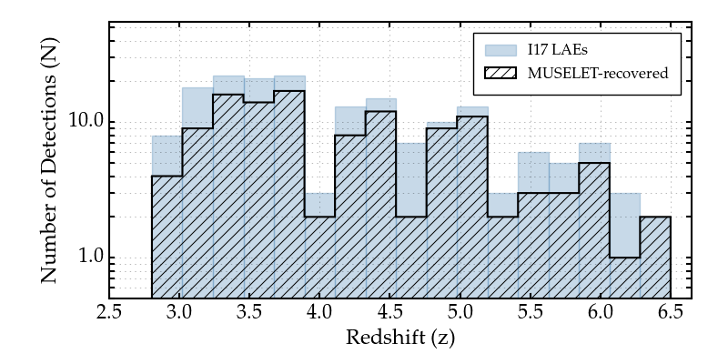
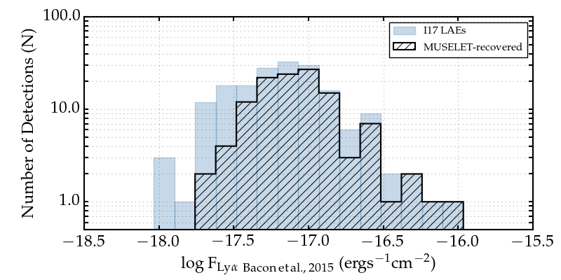
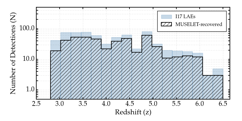
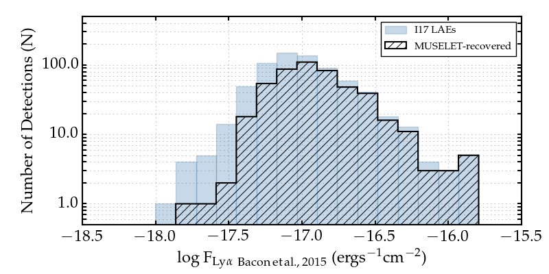
Figure 1: Detections using our detection software muselet, overplotted on the LAEs discovered and catalogued in I17. In the left-hand panels (upper udf-10, lower mosaic) we show the redshift distributions, demonstrating an even recovery rate across the entire redshift range. In the right-hand panels (upper udf-10, lower mosaic) we use the published flux estimates of I17 to show the distribution of fluxes recovered by muselet vs the distribution for I17 LAEs.

Detecting galaxies by virtue of their Ly$\alpha$ emission however, gives us access to the low-mass end of the star-forming galaxy population which we now believe were the dominant population in the early Universe. Some of the galaxies detected this way would otherwise be completely un-detected even in deep HST photometry (Bacon et al. 2015, Drake et al. 2017). Given a statistical sample of objects, one can characterise the population by examining the number of objects as a function of their luminosity - the luminosity function, often fit with a Schechter function parametrised by $\alpha$, $\phi^{*}$ and $L^{*}$ (Schechter 1976). This gives us characteristic values of the faint-end slope, number density, and luminosity, respectively, and can be used to describe the nature of the population at a particular redshift and to examine its evolution.

An efficient way to select large samples of star-forming galaxies is through narrowband selection, whereby a narrow filter is used to select objects displaying an excess in flux relative to the corresponding broad band filter (e.g. thousands of H$\alpha$, H$\beta$, [Oiii] and [Oii] emitters at $z<2$ have been presented in Sobral et al. 2013, Drake et al. 2013 and Drake et al. 2015).

Despite the success of this technique, at high redshift where the Ly$\alpha$ line is accessible to optical surveys the samples rarely probe far below $L^{*}$ and it is usually necessary to make some assumption as to the value of the faint-end slope $\alpha$, a key parameter for assessing the number of faint galaxies available to power reionisation in the early Universe. (Rhoads et al. 2000, Ouchi et al. 2003, Hu et al. 2004, Ouchi et al. 2008, Yamada et al. 2012, Matthee et al. 2015, Konno et al. 2016, Santos et al. 2016)

An alternative approach to LAE selection, was pioneered by Martin et al. (2008), and subsequently exploited in Dressler et al. (2011), Henry et al. (2012) and Dressler et al. (2015), combining a narrowband filter with 100 long slits – multislit narrowband spectroscopy. With this technique the authors found evidence for a very steep faint-end slope of the luminosity function, confirmed by each subsequent study, although they note that this is a sensitive function of the correction they make for foreground galaxies. With this method, and taking fiducial values for the escape of Ly$\alpha$, the escape of Lyman continuum (LyC) and the clumping of the IGM they determined that LAEs probably produce a significant fraction of the ionising radiation required to maintain a transparent IGM at $z=5.7$.

Some of the very deepest samples of LAEs to date come from blind long-slit spectroscopy, successfully discovering LAEs reaching flux levels as low as a few $\times 10^{-18}{\rm{erg\,s}}^{-1}{\rm{cm}}^{-2}$ for example Rauch et al. (2008), although this required $92$ hours integration with ESO-VLT FORS2, and the idenitifcation of many of the single line emitters was again ambiguous. Reaching a similar flux limit, Cassata et al. (2011) combined targetted and serendipitous spectroscopy from the VIMOS-VLT Deep Survey (VVDS) to produce a sample of 217 LAEs across the redshift range $2.00\leq z\leq 6.62$. They split their sample into three large redshift bins, and looked for signs of evolution in the observed luminosity function across the redshift range. In agreement with van Breukelen et al. (2005), Shimasaku et al. (2006), and Ouchi et al. (2008) they found no evidence of evolution between the redshift bins within their errors. Due to the dynamic range of the study, Cassata et al. (2011) fixed $\phi^{*}$ and $L^{*}$ in their lowest two redshift bins and used the $1/$V_max estimator to measure $\alpha$, finding shallower values of the faint-end slope than implied by the number counts of Rauch et al. (2008) or Martin et al. (2008), Dressler et al. (2011), 2015, and Henry et al. (2012). Similarly in the highest redshift bin they fixed the value of $\alpha$, fitting only for $\phi^{*}$ and $L^{*}$, although interestingly they found the measured value of $\alpha$ increased from their lowest redshift bin to the next. Deep spectroscopic studies are needed to evaluate the faint end of the luminosity function, however each of the efforts to date suffer from irregular selection functions which are difficult to reproduce, and flux losses which are difficult to quantify and correct for.

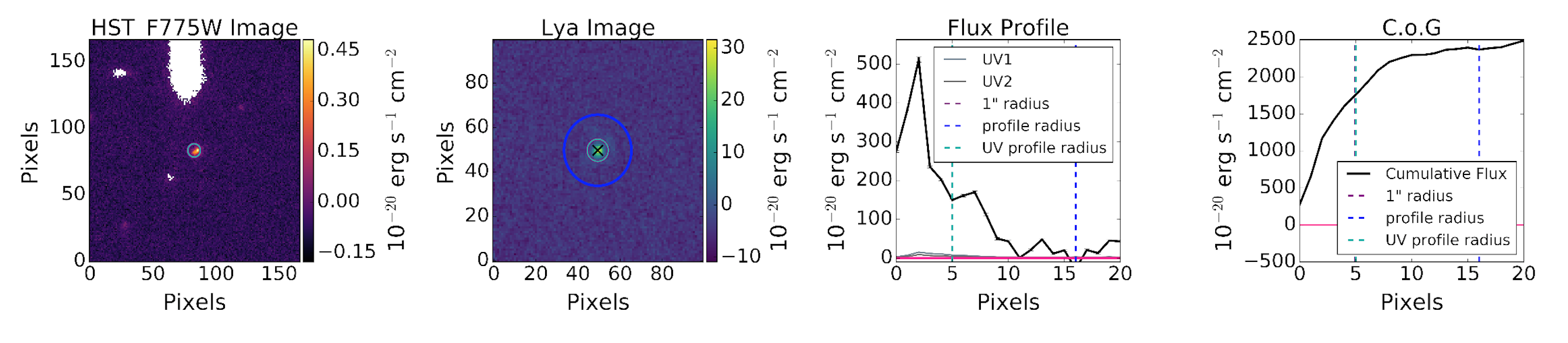
Figure 2: Example of flux estimation for object 149 in the udf-10 field. In the first panel we show the HST image corresponding to the wavelength of Ly$\alpha$, in the second panel we show the narrowband image extracted from the MUSE cube. In the third panel we show the flux profile of the galaxy determined according to the method described in Section 3.0.1, and in the fourth panel we show the cumulative flux determined by summing the results in Section 3.0.1. The dashed vertical lines in the third and fourth panels show the $1\arcsec$ radius, and the different radii encompassing the total flux according to a curve of growth analysis on either the HST or the MUSE images.

The advent of the Multi Unit Spectroscopic Explorer (MUSE; Bacon et al. 2010), on the Very Large Telescope (VLT), provides us with a way to blindly select large samples of spectroscopically-confirmed LAEs in a homogeneous manner (Bacon et al. 2015, Drake et al. 2017) as well as probing the lensed LAE populations behind galaxy clusters (Bina et al. 2016, Smit et al. 2017). In addition to the ability of MUSE to perform as a ‘detection machine’ for star-forming galaxies, the deep datacubes allow us to establish reliable total Ly$\alpha$ line fluxes by ensuring we capture the total width of the Ly$\alpha$ line in wavelength, and the full extent of each object on-sky. Indeed, Ly$\alpha$ emission has now increasingly been found to be extended around galaxies, which has implications for our interpretation of the luminosity function. Steidel et al. (2011) first proposed extended Ly$\alpha$ emission may be a generic property of high redshift star-forming galaxies, which was confirmed by Momose et al. (2014) who found scale lengths $\approx 5-10$ kpc, but the emission was not detectable around any individual galaxy (see also Yuma et al. 2013 and Yuma et al., submitted, for individual detections of metal-line blobs at lower $z$ from the sample of Drake et al. 2013). Wisotzki et al. (2016) were the first to make detections of extended Ly$\alpha$ halos around individual high-redshift galaxies, uncovering $21$ halos amongst $26$ isolated LAEs presented in Bacon et al. (2015).

In this paper we build on the procedure developed in Drake et al. 2017 (hereafter D17a) and upgrade our analysis in the ways outlined below. We push our detection software muselet to lower flux limits by tuning the parameters. We incorporate a more sophisticated completeness assessment than in D17a, by simulating extended Ly$\alpha$ emitters and performing a fake source recovery experiment. We test and correct for the effect of bias in our flux measurements of faint sources, and finally we implement two different approaches to assessing the Ly$\alpha$ luminosity function. The paper proceeds as follows: in Section 2 we introduce our survey of the MUSE Hubble Ultra Deep Field; HUDF (Bacon2017; hereafter B17) and our catalogue construction from the parent data set (presented in Inami2017; hereafter I17). In Section 3 we describe our approach to measuring accurate total Ly$\alpha$ fluxes, and describe our method for constructing realistic extended LAEs in Section 4 to assess the possible bias introduced in our flux measurements and to evaluate the completeness of the sample. In Section 5 we present two alternative approaches to assessing the Ly$\alpha$ luminosity function, first using the $1/$V_max estimator, and secondly a maximum likelihood approach to determine the most likely Schechter parameters describing the sample. We discuss in Section 6 the evolution of the observed luminosity function, the contribution of LAEs to the overall star formation rate density across the entire redshift range, and finally the ability of LAEs to produce enough ionising radiation to maintain an ionised IGM at redshift $5.00\leq z<6.64$.

Throughout the paper we assume a $\Lambda$CDM cosmology, $H_{0}=70.0$ kms^-1 Mpc^-1, $\Omega_{m}=0.3$, $\Omega_{\Lambda}=0.7$.

2 Data and catalogue construction

2.1 Observations

As part of the MUSE consortium Guaranteed Time Observations we observed the Hubble Ultra Deep Field (HUDF) for a total of 137 hours in dark time with good seeing conditions (PI: R.Bacon). The observing strategy consisted of a ten-hour integration across a $3\arcmin\times 3\arcmin$ mosaic consisting of $9$ MUSE pointings, and overlaid on this, a $30$ hour integration across a single MUSE pointing ($1\arcmin\times 1\arcmin$).Details on observing strategy and data reduction are given in Bacon et al. 2017 (hereafter B17). MUSE delivers an instantaneous wavelength range of $4750-9300\,\AA$ with a mean spectral resolution of R $\approx 3000$, and spatial resolution of 0.202″pix^-1.

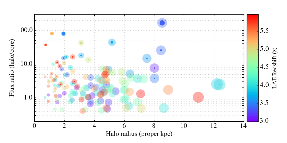
Figure 3: Halo properties used to simulate our realistic fake LAEs. The halos are entirely characterised by two quantities, the halo scale length in proper kpc, and the flux ratio between the halo and the core. Measurements are taken from those presented in L17 and W16. Each halo is depicted as an extended disk of size proportional to the halo extent, overlaid with a compact component of size inversely proportional to the flux ratio, this gives an easy way to envisage the properties of the observed halos.

2.2 Catalogue construction

As we discussed at length in D17a, to assess the luminosity function it is imperative to construct a sample of objects using a simple set of selection criteria which can easily be reproduced when assessing the completeness of the sample. Without fulfilling this criterion it is impossible to quantify the sources missed during source detection and therefore impossible to reliably evaluate the luminosity function. For this reason we do not rely solely on the official MUSE-consortium catalogue release (I17) - while the catalogue is rich in data and deep, the methods employed to detect sources are varied and heterogeneous, resulting in a selection function which is impossible to reproduce. We instead choose to implement a single piece of detection software, muselet, (J.Richard) and validate our detections through a full 3D match to the deeper catalogue of I17. We note that detection alogithms in survey data always require some trade off to be made between sensitivity and the number of false detections, and with a view to assessing the luminosity function, the need for a well-understood selection function outweighs the need to detect the faintest possible candidates (which are in principle ambiguous, producing a less certain result than with a fully characterised selection function).

We follow the procedure outlined in D17a to go from a catalogue of muselet emission-line detections to a catalogue of spectroscopically confirmed LAEs. The details are outlined below, and further information can be found in D17a.

2.2.1 Source detection

muselet begins by processing the entire MUSE datacube applying a running median filter to produce continuum-subtracted narrowband images at each wavelength plane. Each image is a line-weighted average of $5$ wavelength planes ($6.25\AA$ total width) with continuum estimated and subtracted from two spectral medians on either side of the narrowband region ($25\AA$ in width). muselet then runs the SExtractor package (Bertin & Arnouts 1996) on each narrowband image as it is created using the exposure map cube as a weight map.

Once the entire cube is processed, muselet merges the detections from each narrowband image to create a catalogue of emission lines. Lines which are co-incident on-sky within $4$ pixels ($0.8\arcsec$) are merged into single sources, and an input catalogue of rest-frame emission-line wavelengths and flux ratios is used to determine a best redshift for sources with multiple lines, the remainder of sources displaying a single emission line are flagged as candidate LAEs. Thanks to the wavelength coverage of MUSE, we anticipate the detection of multiple lines for sources exhibiting H$\alpha$, H$\beta$ or [Oiii] emission meaning that only the [Oii] doublet is a potential contaminant of the single-line sample.

2.2.2 Final catalogue

Each of our muselet detections is validated through a 3D match to I17, requiring sources to be coincident on-sky ($\Delta$ RA, $\Delta$ DEC $<1.0\,\arcsec$) and in observed wavelength ($\Delta\,\lambda<6.25\AA$).

We investigated the setup of both SExtractor and muselet parameters that would optimise the ratio of matches to the total number of muselet detections. The results of these experiments led to our lowering the muselet clean threshold to $0.4$ - meaning that only parts of the cube with fewer than $40\%$ of the total number of exposures were rejected by the software. Additionally, the SExtractor parameters detect minarea, and detect thresh (minimum number of contiguous pixels above the threshold and detection-$\sigma$ respectively) were each lowered to $=2.0$ from our previous stricter requirements of $3.0$ and $2.5$ in D17a. Naturally, the cost of lowering our detection thresholds is to increase the number of false detections from muselet (which were negligible in the pilot study), and as such our completeness estimates here could be slightly overestimated.

Our match to I17 confirmed that $123$ and $481$ single line sources were LAEs in the udf-10 and mosaic fields respectively. In Figure 1 we show the parent sample from I17 in blue, overlaid with the muselet-detected sample depicted by a black hatched histogram. In the two left-hand panels we show LAEs as a function of redshift demonstrating a flat distribution of objects across the entire redshift range, and no sytematic bias in the way we select our sample. In the two right-hand panels we show LAEs as a function of the Ly$\alpha$ flux estimates presented in I17. With our re-tuning of the muselet software we now recover LAEs as faint as a few $\times 10^{-18}{\rm{erg\,s}}^{-1}{\rm{cm}}^{-2}$.

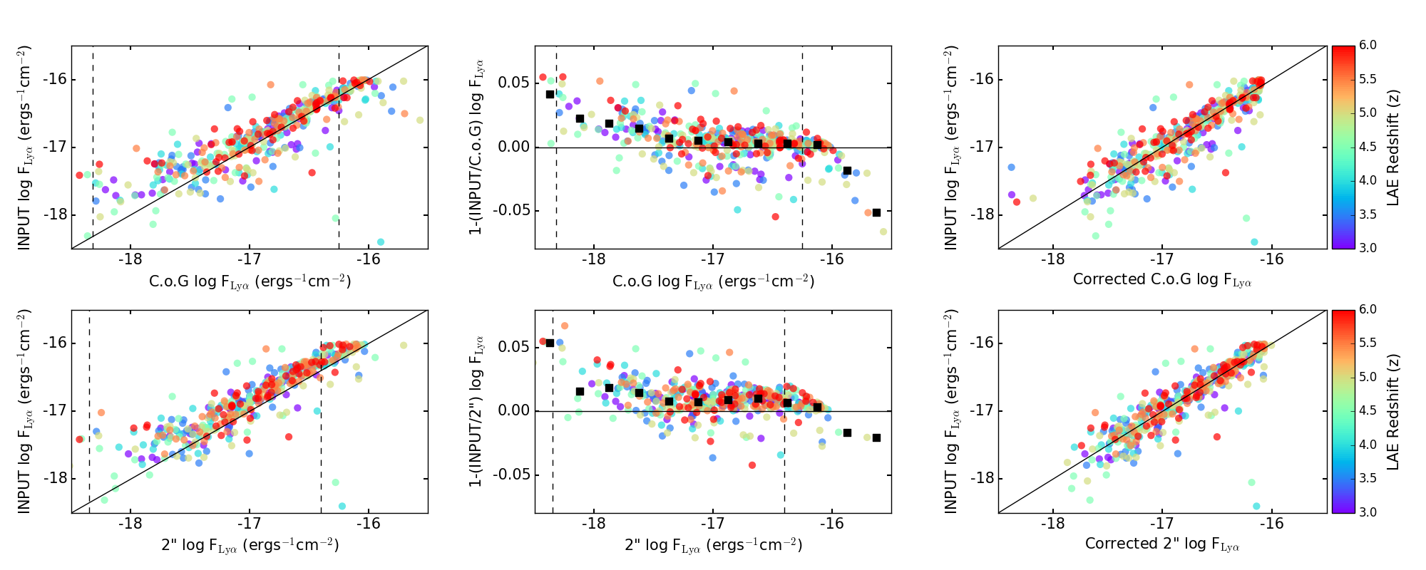
Figure 4: Bias in flux estimation for C.o.G (upper row) and 2” aperture (lower row) measurements in the UDF-10 field. In the first column of panels we show a comparison between the input total flux on the ordinate and the recovered flux on the abscissa. In the central column of panels we show the difference between input and recovered flux on the ordinate as a function of recovered flux on the abscissa, where the black squares indicate the median value of the offset, which increases rapidly towards lower fluxes. In each of the first two columns of panels we depict the minimum and maximum fluxes of objects detected in the MUSELET catalogue with dashed lines. In the final column of panels we show values of measured flux corrected for the median offset using measurements from the central columns.

3 Flux measurements

The accurate measurement of Ly$\alpha$ fluxes has proved to be non-trivial. Furthermore, the definition of the Ly$\alpha$ flux itself is changing now that we are working in the regime where LAEs are seen to be extended objects often with diffuse Ly$\alpha$-emitting halos. Here we work mainly with our best estimates of the total Ly$\alpha$ flux for each object, that is, including extended emission in the halos of galaxies.

In section $3$ of D17a, we discussed the most accurate way to determine total Ly$\alpha$ fluxes and argued that a curve-of-growth approach provided the most accurate estimates. Here, we again investigate the curve-of-growth technique, but before developing a more advanced analysis, we consider the possible bias that might be inherent to this method in our ability to fully recover flux according to the true total flux. The approach developed to correct for this bias is described in Section 4.1.

This work upgrades the preliminary analysis presented in D17a to make use of the MUSE-HUDF data-release source objects. For each source found by muselet with a match in the catalogue of I17 we take the source objects provided in the data release, and measure the FWHM of the Ly$\alpha$ line on the 1D spectrum. We then add two larger cutouts of $20\arcsec$ on a side to each source object from the full cube – a narrowband and a continuum image. The narrowband image, centred on the wavelength of the detection, is of width $4\times$ the FWHM of the line, and the continuum image is $200\AA$ wide, offset by $150\AA$ from the peak of the Ly$\alpha$ detection. By subtracting the broadband from the narrowband image we construct a “Ly$\alpha$ image” (continuum-subtracted narrowband image) and it is on this image that we perform all photometry.

3.0.1 Curve of growth

We use the python package photutils to prepare the Ly$\alpha$ image by performing a local background subtraction, and masking neighbouring objects in the Ly$\alpha$ image. Then taking the muselet detection coordinates to be the centre of each object, we place consecutive annuli of increasing radius on the object, taking the average flux in each ring as we go, multiplied by the full area of the annulus. When the average value in a ring reaches or dips below the local background, we sum the flux out to this radius as the total Ly$\alpha$ flux.

3.0.2 Two arcsecond apertures

We prepare the image in the same way as for the curve-of-growth analysis, and again take the muselet coordinates as the centre of the Ly$\alpha$ emission. Working with the same set of consecutive annuli we simply sum the flux for each object when the diameter of the annulus reaches $2\arcsec$. We note that this produces an ever so slightly different result to placing a $2\arcsec$ aperture directly on the image.

4 Simulating realistic extended LAEs

In D17a we based our fake source recovery experiments on point-source line-emitters using the measured line profiles from the galaxies presented in our study of the Hubble Deep Field South (Bacon et al. 2015). While the estimates provided a handle on the completeness of the study, we noted that the reality of extended Ly$\alpha$ emission might make some significant impact on the recovery fraction of LAEs (see Herenz et al). Additionally, our completeness estimates are based on the input Ly$\alpha$ flux, and so it is prudent to understand the relationship between measured fluxes and the most likely intrinsic flux. To address both the issue of completeness of extended LAEs and the question of some bias in the recovery of total Ly$\alpha$ flux we designed a fake source recovery experiment using “realistic” fake LAEs. We model extended Ly$\alpha$ surface brightness profiles with no continuum emission, making use of the detailed measurements of Leclercq2017 (hereafter L17) performed on all Ly$\alpha$ halos detected in the MUSE HUDF observations, and Wisotzki et al. (2016) on those in the HDFS. Both L17 and Wisotzki et al. (2016) follow a similar procedure to decompose the LAE light profiles, invoking a “continuum-like” core component, and a diffuse, extended halo.

We approximate the central continuum-like component as a point source, and combine this with an exponentially declining profile to represent the extended halo. The emitters can then be entirely characterised by two parameters; the halo scale length in proper kpc, and the flux ratio between the halo and the core components. Figure 3 shows the distribution of halo parameters used in the simulation. The extent of the halo in proper kpc is given on the abscissa, and the flux ratio between the extended halo component and the compact continuum-like component is given on the ordinate, with colours indicating the redshift of the halo observed by Wisotzki et al. (2016) or L16. We depict each halo as an extended disk of size proportional to the halo extent, overlaid with a compact component of size inversely proportional to the flux ratio, this gives an easy way to envisage the properties of the observed halos. For each of our experiments, described below, we draw halo parameters from the measured sample in a large redshift bin ($\Delta z\approx 1$) centred on the input redshift of the simulated halo.

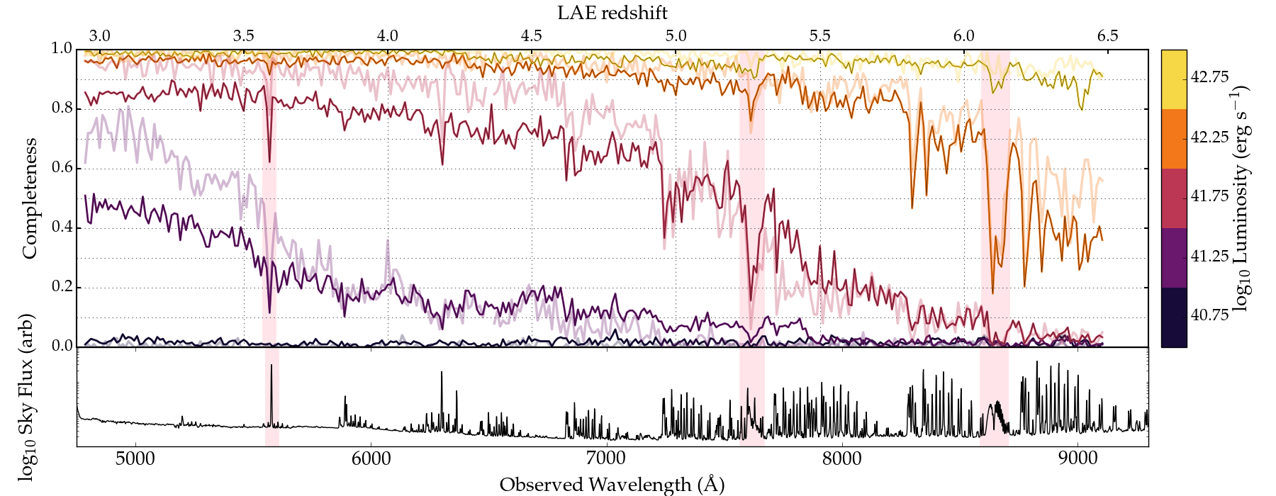
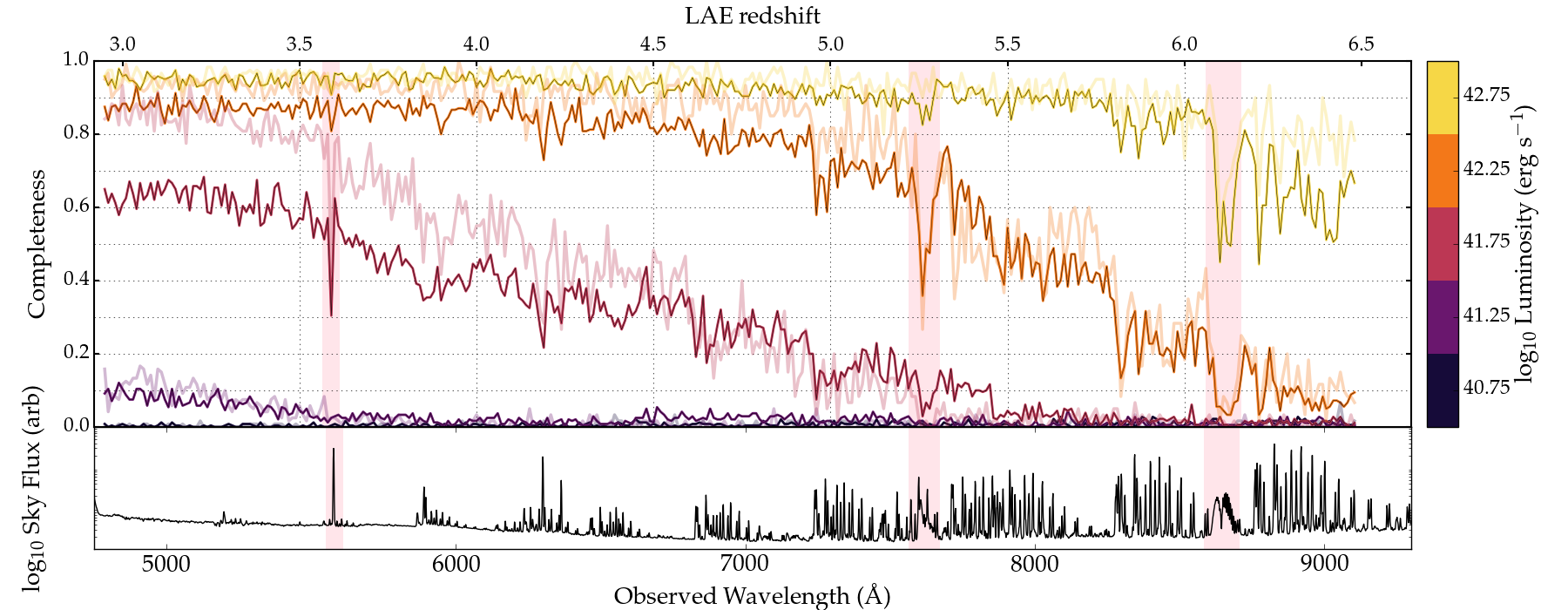
Figure 5: The recovery fraction of LAEs with our detection software as a function of observed wavelength, and LAE-redshift denoted on the top axis for the udf-10 (top), and the mosaic (bottom) fields. Colours represent the input luminosity of the fake LAEs, dark lines reinforced in black show the recovery of extended objects, and pale lines show point sources of the same total luminosity. In the lower panel of each plot the night sky is shown, and areas where sky lines most severely affect our recovery are highlighted in pink.

4.1 Flux recovery of simulated emitters

In Drake et al. (2017) we discussed the difference in the apparent luminosity function when using different approaches to estimate total Ly$\alpha$ flux. We concluded that using a curve-of-growth analysis provided the most accurate measure of F_Lyα although noted that this approach introduced the possibility of a bias in the fraction of the flux recovered according to true total flux.

Here, we inserted fake sources with a wide range of input fluxes and randomly drawn halo parameters at a series of discrete redshifts. For those objects that were recovered by our detection software we could then apply the same methods of flux estimation that we employed for the sample of real objects to uncover any systematic bias in the way we estimate total Ly$\alpha$ fluxes. The results of this experiment are presented in Figure 4 for the udf-10 field.

Interestingly, the curve-of-growth recovers the total input flux remarkably well at bright fluxes, but has a huge scatter at lower fluxes rendering it completely unreliable, although not systematically wrong. Secondly, the 2$\arcsec$ measurements seem to work fairly well at lower fluxes, but diverge systematically ar higher flux levels (as we discussed in D17a).

For each of these two approaches to flux recovery, we calculate the median offset of the recovered fluxes from the input fluxes, and interpolate the values in order to make statistical correction as a function of recovered flux to the measured values. In the final column of panels in Figure 4 we show the corrected values for first the curve-of-growth, and then the $2\arcsec$ apertures for measurements on the udf-10 field. It can be seen in these plots that while both estimates are now centred on an exact correlation between input and recovered flux, the scatter in the $2\arcsec$ measurements is much lower than that in the corrected curve-of-growth values. For this reason it is the corrected $2\arcsec$ aperture flux values which we propagate to the luminosity functions. We find a typical offset of $0.02$ in log F (erg s^-1 cm^-2) with an average r.m.s of $0.008$.

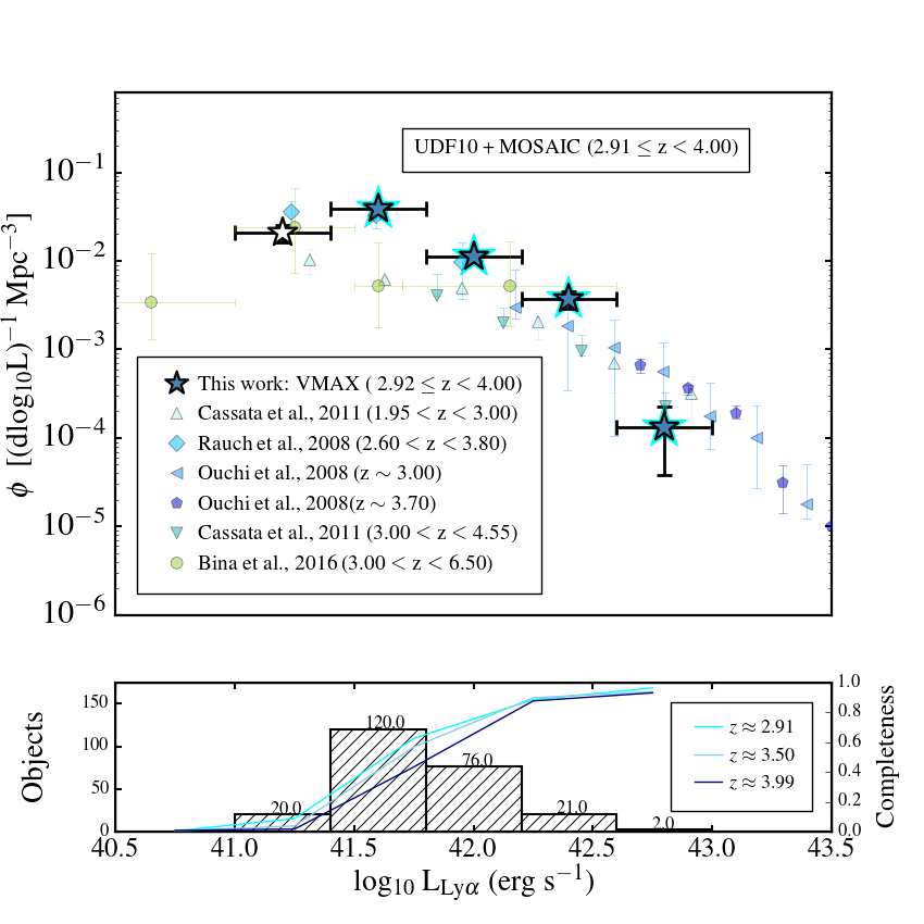
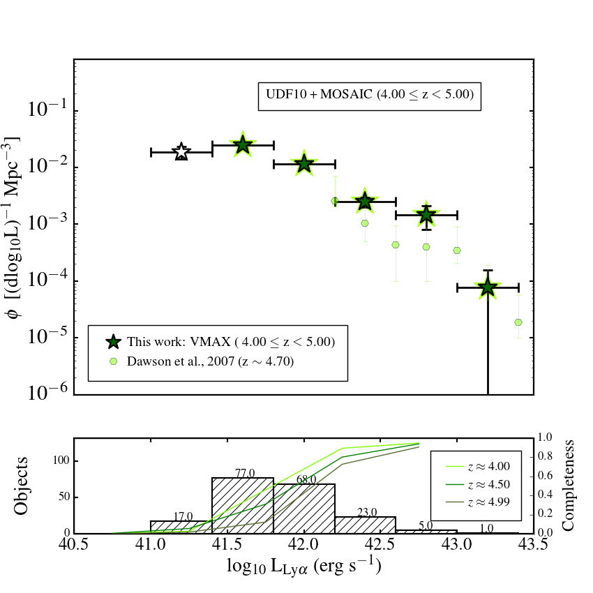
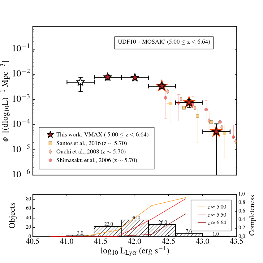
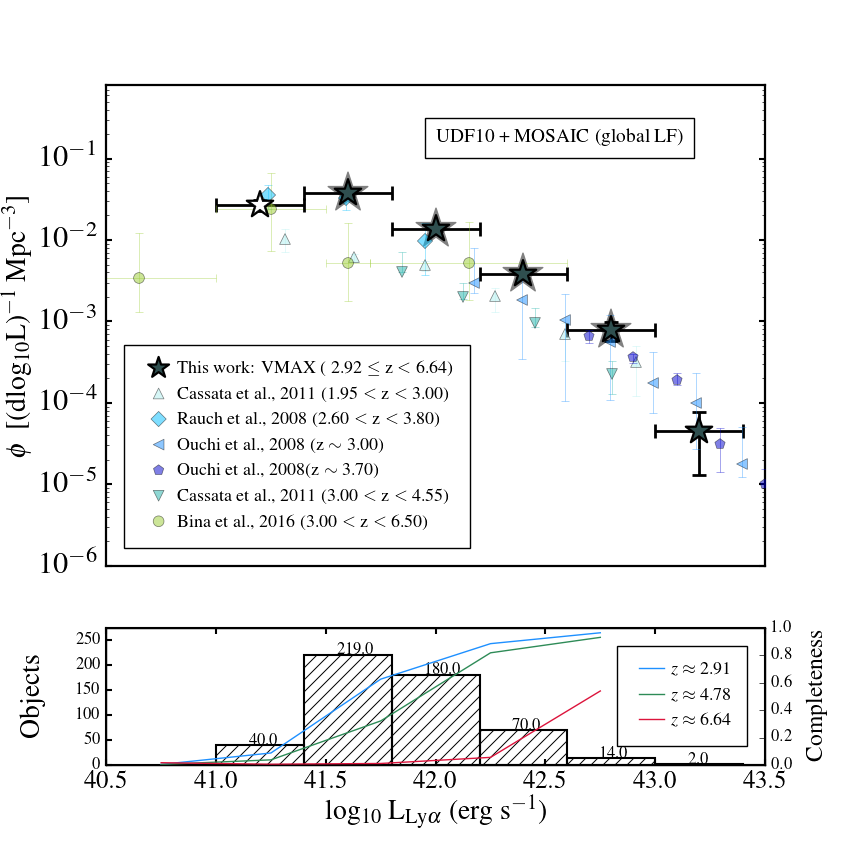
Figure 6: Number densities resulting from the $1/$V_max estimator. Top left: ($2.91\leq z<4.00$) bin; blue, top right ($4.00\leq z<5.00$); bin green, bottom left ($5.00\leq z<6.64$); bin red, bottom right all LAEs ($2.91\leq z<6.64$). In each panel we show number densities in bins of 0.4 dex, together with literature results at similar redshifts from narrowband or long-slit surveys. In the lower part of each panel we show the histogram of objects in the redshift bin overlaid with the completeness estimate for extended emitters at the lower, middle and highest redshift in each bin. In each panel we flag incomplete bins with a transparent datapoint. Errorbars represent the $1\sigma$ Poissonian uncertainty, we note that often the ends of the bars are hidden behind the data point itself.

4.2 Fake source recovery

We follow the procedure described in D17a, working systematically through the cube adding fake emitters in redshift intervals of $\Delta z=0.01$. This time we use two different setups designed to facilitate two different approaches to estimating the luminosity function - the first using 5 luminosity bins, and the second using flux intervals of $\Delta f=0.05$ (erg s^-1 cm^-2). The incorporation of the completeness estimates into the luminosity functions is described in Section 5. For each fake LAE inserted into the cube, observed pairs of values of scale length and flux ratio are drawn from the measurements presented in Wisotzki et al. (2016) and L16. For each redshift-flux and redshift-luminosity combination we run our detection software muselet using exactly the same setup as described in Section 2.2.1, and record the recovery fraction of fake extended emitters.

5 Luminosity functions

Here we implement two different estimators to assess the luminosity function, each with their own strengths and weaknesses. With a view to estimating the number density of objects in bins of luminosity, the $1/$V_max estimator provides a simple way to visualise the values and makes no prior assumption as to the shape of the function. We discuss the limitations of this approach in our pilot study of the HDFS; D17a. In terms of parameterising the luminosity function, fits to binned data are to be interpreted with caution, and an alternative approach is preferred. Here, we use the maximum likelihood estimator following the formalism described in Marshall et al. 1983 (and applied in Drake et al. 2013 and Drake et al. 2015 to narrowband samples).

One advantage of the MUSE mosaic of the HUDF is that the $3\times 3$ square arcminute field in combination with the $10$-hour integration time, provides the ideal volume to capitalise on the trade-off between minimising cosmic variance and probing the bulk of the LAE population (Garel et al. 2016). This allows us to draw more solid conclusions than those from our $1\times 1$ pilot study of the HDFS field (Drake et al. 2017).

5.1 1/Vmax estimator

We assess the luminosity function in $3$ broad redshift bins ($2.91\leq z<4.00$), ($4.00\leq z\leq 4.99$) and ($5.00\leq z<6.64$) in addition to the ‘global’ luminosity function ($2.91\leq z\leq 6.64$) for LAEs in the combined UDF-10 plus mosaic field through use of the $1/V_{{\rm{max}}}$ estimator. The results, discussed further below, are presented in Table 2 and Figure 6.

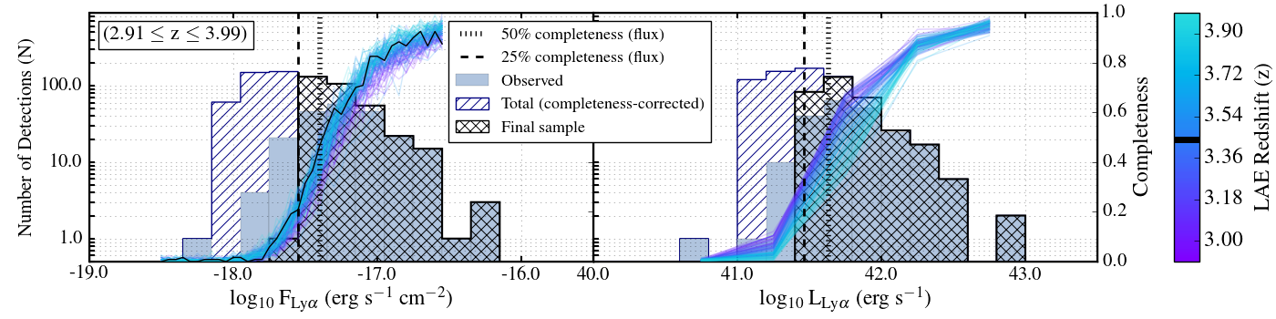
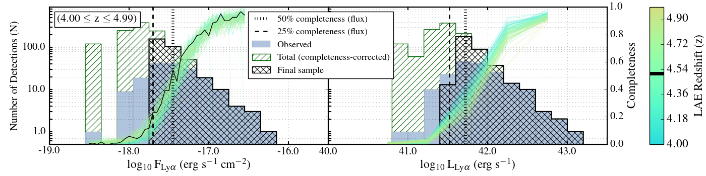
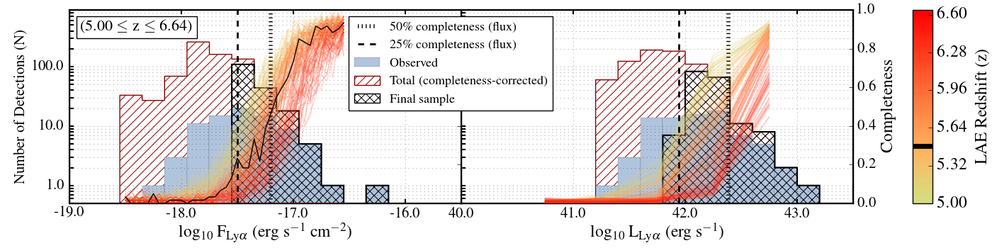
Figure 7: Flux and log-luminosity distributions of objects from the mosaic in three broad redshift bins at ($2.91\leq z<4.00$), ($4.00\leq z\leq 4.99$) and ($5.00\leq z<6.64$). In each panel we show the total distribution of objects (including fakes created and added to the sample through the process described in Section 5.2) in a coloured hatched histogram. We overlay the distribution of observed objects in filled blue bars. The final samples, curtailed at the $25\%$ completeness limit in flux ($\Delta\,f=0.05$) for the median redshift of objects in the redshift bin is overplotted in a bold cross-hatched black histogram. Overlaid on each panel are the completeness curves as a function of flux (or log luminosity) at each redshift ($\Delta\,z=0.01$) falling within the bin. Each redshift is given by a different coloured line according to the colour-map shown in the colour bar, and the curve at the median redshift of the bin is emphasized in black. The median redshift of the bin is also given by a black line on the colour bar.

5.1.1 Completeness correction

To implement the $1/$Vmax estimator, it is necessary to evaluate the completeness of the sample for a given luminosity as a function of redshift. In Figure 5 we show the recovery fraction of LAEs with muselet as a function of observed wavelength at $5$ values of log luminosity, giving the corresponding LAE-redshift on the top axis. The night sky spectrum from MUSE is shown in the lower panel, and colour-coding of the lines represents the in-put luminosity of the sources ranging between $41.0<$ log $L$ (erg s${}^{-1})<43.0$ at each wavelength of the cube in intervals of $\Delta\lambda=12\AA$. In the upper panel we show the recovery fraction from the deep $1\arcmin\times 1\arcmin$ udf-10 pointing inserting $20$ LAEs at a time in a $z$-$L$ bin.

The effects of night sky emission are most evident at luminosities up to log $L$$\approx 42.5$. The prominent [Oi] airglow line at $5577\AA$ however impacts recovery even at the brightest luminosities in our simulation. The broader absorption features at $7600\AA$ and $8600\AA$ also make a strong impact on detection efficiency across the full range of luminosities. Importantly, the difference between the recovery fractions of point-like and extended emitters is evident. For each coloured line of constant luminosity, we show two different recovery fractions; the extended emitter recovery fraction, and the point-source recovery fraction. It is obvious that for a given total luminosity the point-like emitters are recovered more readily than the extended objects meaning that our previous recovery experiements will have overestimated the completeness of the sample.

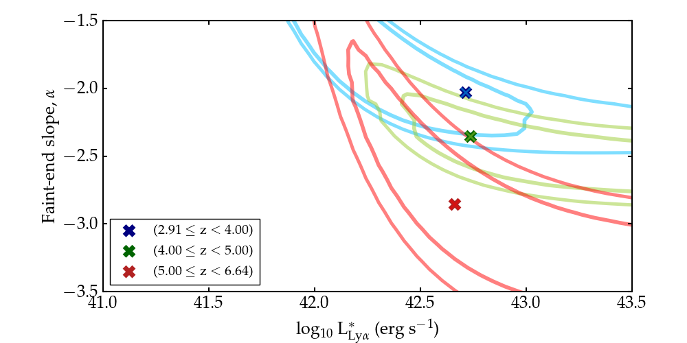
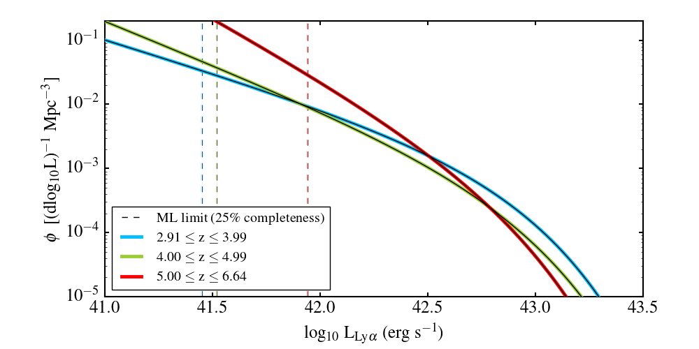
Figure 8: Maximum likelihood Schechter luminosity functions for three redshift bins ($2.91\leq z<4.00$); blue, ($4.00\leq z<5.00$); green, ($5.00\leq z<6.64$); red. In the upper panel we show 68% and 95% joint confidence regions which correspond to $\Delta$ S $=2.30$ and $6.18$ for two free fit parameters (L^∗ and $\alpha$). In the lower panel we show the maximum likelihood Schechter functions as solid lines.

5.1.2 1/Vmax formalism

For each LAE, i, in the catalogue, the redshift, $z_{\,i}$, is determined according to $z_{\,i}={\lambda_{\,i}}/({1215.67}-1.0)$, where $\lambda_{\,i}$ is the observed wavelength of Ly$\alpha$ according to the peak of the emission detected by muselet. The luminosity $L_{i}$ is then computed according to $L_{i}=f_{i}4\pi D_{L}^{2}(z_{i})$, where $f_{i}$ is the corrected Ly$\alpha$ flux measured in a $2\arcsec$ aperture, $D_{L}$ is the luminosity distance, and $z_{i}$ is the Ly$\alpha$ redshift. The maximum co-moving volume within which this object could be observed, $V_{{\rm{max}}}$($L_{\>i}$, $z$), is then computed by:

$${V_{{\rm{max}}}(L_{i},z)=\int_{z1}^{z2}\frac{{\rm{d}}V}{{\rm{d}}z}\,{\rm{C}}(L_{i},z)\,{\rm{d}}z,}$$ (1)

where $z_{1}$ and $z_{2}$, the minimum and maximum redshifts of the bin respectively, d$V$ is the co-moving volume element corresponding to redshift interval d$z=0.01$, and C($L_{i}$, $z$) is the completeness curve for an extended object of total luminosity $L_{i}$, across all redshifts $z_{i}$.

The number density of objects per luminosity bin, $\phi$, is then calculated according to:

$${\phi[({\rm{dlog_{10}}}L)^{-1}{\rm{Mpc}}^{-3}]=\sum_{i}\frac{1}{V_{\rm{max}}(L_{i},z_{i})}/{\rm{binsize}}.}$$ (2)

5.1.3 1/Vmax comparison to literature

With an improved estimate of completeness from the realistic extended emitters we see in Figure 6 that the LF is steep down to log luminosities of $L$$<41.5$ erg s^-1, and sits increasingly higher than literature results towards fainter luminosities. This is entirely expected due to our improved completeness correction following the analysis in D17a, and consistent with the scenario in which the ability of MUSE to capture extended emission results in a luminosity function showing number densities systematically above previous literature results by a factor of $2$-$3$. In each panel of Figure 6 the redshift range is given in the upper right-hand corner, number densities from this work are depicted, plotted together with literature data across a similar redshift range identified in the key. Each data point from MUSE is shown with a Poissonian error on the point. In the lower part of each panel we show the histogram of objects’ luminosities in the redshift bin, and overplot the the completeness as a function of luminosity at the lowest, central and highest redshifts contained in the luminosity function. This is intended to allow the reader to interpret each luminosity function with the appropriate level of caution - for instance in the highest redshift bin more than half the bins of luminosity consist of objects where a large completeness correction will have been used on the majority of objects, and hence there is a large associated uncertainty.

In the ($2.91\leq z<4.00$) bin, our data alleviate the discrepancy between the two leading studies at redshift $\approx 3$ from VVDS (Cassata et al. 2011) and Rauch et al. (2008). Our data points sit almost exactly on top of those from Rauch et al. (2008) confirming that the majority of single line emitters detected in their $90$-hour integration were LAEs. In the ($4.00\leq z<5.00$) bin our data are over $1$ dex deeper than the previous study at this redshift (Dawson et al. 2007), we are in agreement with their number densities within our error bars at all overlapping luminosities, and our data show a continued steep slope down to $L$$<41.5$ erg s^-1. In our highest redshift bin, ($5.00\leq z<6.64$), our data are a full $1.5$ dex deeper than previous studies. The data turn over in the bins below $L$$<42$ erg s^-1 but errors from the completeness correction to objects in these bins is large since values of completeness are well below $50\%$ for all luminosities in the bins in this redshift range. Finally we show the ‘global’ luminosity function across the redshift range ($2.91\leq z\leq 6.64$) in the final panel together with literature studies that bracket the same redshift range, and the two narrowband studies from Ouchi et al. (2003) and Ouchi et al. (2008) which represent the reference samples for high-redshift LAE studies.

Table 1: Maximum likelihood Schechter luminosity functions for LAEs in the mosaic field. Marginal 68% confidence intervals on single parameters are taken from the extremes of the $\Delta\,S=1$ contours. The 68% confidence intervals on the luminosity density and SFRD however depend on the joint confidence interval the two free parameters L^∗ and $\alpha$ ($\Delta\,S=2.30$ contour as in Figure 8) - details in Section 5.3. We note that as our sample are almost entirely below L^∗, the value of L^∗ itself is only loosely constrained by our data, and hence we only find a single bound of the 68% confidence intervals for the Schechter parameters in two redshift bins. Thankfully this is not a problem for the luminosity density and SFRD, as the extreme values are reached in a perpendicular direction to the length of the ellipses.

z	Volume	Real objects†	Total†	log10$\phi^{*}$	log10$L^{*}$	$\alpha$	log $\rho_{Ly\alpha}$††	SFRD††
	$10^{4}$ Mpc-3			(Mpc-3)	(erg s-1)		(erg s-1Mpc-3)	(M⊙ yr-1Mpc-3)
( 2.92$\leq z\leq$ 3.99)	3.10	193	328	-3.10${}^{+1.37}_{-0.45}$	42.72${}^{+0.23}_{-0.97}$	-2.03${}^{+1.42}_{-0.07}$	40.154${}^{+0.346}_{-0.138}$	0.014${}^{+0.017}_{-0.004}$
( 4.00$\leq z\leq$ 4.99)	2.57	144	346	-3.42${}^{+0.51}_{-\infty}$	42.74${}^{+\infty}_{-0.19}$	-2.36${}^{+0.17}_{-\infty}$	40.203${}^{+0.397}_{-0.002}$	0.015${}^{+0.023}_{-0.000}$
( 5.00$\leq z\leq$ 6.64)	3.64	50	176	-3.16${}^{+0.99}_{-\infty}$	42.66${}^{+\infty}_{-0.34}$	-2.86${}^{+0.76}_{-\infty}$	40.939${}^{+0.591}_{-0.727}$	0.083${}^{+0.240}_{-0.067}$
$\dagger>25\%$ completeness in flux at the median redshift of the luminosity function.
$\dagger\dagger$ Integrated to log10 L erg s-1 $=41.0$

5.2 Maximum likelihood estimator

With a view to parameterising the luminosity function we apply the maximum likelihood estimator. Bringing together our bias-corrected flux estimates and our completeness estimates using realistic extended emitters, we can assess the most likely Schechter parameters that would lead to the observed distribution of fluxes. We begin by splitting the data into three broad redshift bins covering the redshift range ($2.91\leq z\leq 6.64$) of $\Delta\,z\approx 1$, and prepare the sample in the following ways.

5.2.1 Completeness correction

As introduced in Section 4.2 we sample the detection completeness on a fine grid of input flux and redshift (or observed wavelength) values with resolution $\Delta\,z=0.01$, and $\Delta f=0.05$ (erg^-1 cm^-2). Considering where our observed data lie on this grid of completeness estimates, we can then correct the number of objects observed at each $z$-$f$ combination to account for the completeness of the survey. It is these completeness-corrected counts that we propagate to the maximum likelihood analysis applying the cuts described below. For a single object which falls at a flux brighter than the grid of combinations tested we interpolate between the completeness at the brightest flux tested at this redshift ($>80\%$ at $-16.5$ erg s${}^{-}1$ cm${}^{-}2$), and an assumed $100\%$ completeness by a flux of $-16.0$ erg s${}^{-}1$ cm${}^{-}2$.

As our data are deep, but covering a small volume of the Universe, our dynamic range is modest $\approx 2.0$ dex and samples well below the knee of the luminosity function. In order to fully exploit the information in the dataset, we can use the number of objects observed in the sample as a constraint on the possible Schecher parameters. This introduces the problem of the uncertainty on the number of objects in the sample where completeness corrections are large. For this reason we choose to cut the sample in each redshift bin at the $25\%$ completeness limit in flux for the median redshift of the objects in each broad redshift bin.

In Figure 7 we show the flux and log-luminosity distributions of objects from the mosaic in the same three broad redshift bins as used for the analysis in Section 5.1. For each row of plots the redshift range is given in the top left-hand corner and three different histograms depict the distribution of fluxes (left-hand column) or log-luminosities (right-hand column). For each panel we show the total distribution of objects (including the completeness-corrected counts) in a coloured hatched histogram. Overlaid on this is the distribution of observed objects in filled blue bars. The final curtailed samples cut at the $25\%$ completeness limit in flux ($\Delta\,f=0.05$) for the median redshift of objects in the redshift bin is overplotted in a bold cross-hatched black histogram.

Overlaid on each panel are the completeness curves as a function of flux (or log luminosity) at each redshift ($\Delta\,z=0.01$) falling within the bin. Each redshift is given by a different coloured line according to the colour-map shown in the colour bar. The median redshift of objects in each redshift range is emphasized in the completeness curves, and on the colour bar. The effect of skylines is again clearly seen in the recovery fraction, this time manifesting as a shift of the entire completeness curve combined with a shallower slope towards the highest redshift LAEs in the cube.

5.2.2 Maximum likelihood formalism

We begin by assuming a Schechter function, written in log form as

$${\phi\,(L)\,{\rm{dlog}}L={\rm{ln10}}\,\phi^{*}\left(\frac{L}{L^{*}}\right)^{\alpha+1}\,e^{-({L}/{L^{*}})}\,{\rm{dlog}}L,}$$ (3)

where $\phi$^∗, $L^{*}$ and $\alpha$ are the characteristic number density, characteristic luminosity, and the gradient of the faint-end slope respectively (Schechter 1976).

Following the method described in Marshall et al. (1983) (and applied in Drake et al. 2013 and Drake et al. 2015 to narrowband samples) we can describe the distribution of fluxes by splitting the flux range into bins small enough to expect no more than 1 object per bin, and writing the likelihood of finding an object in bins F_i and no objects in bins F_j, as Equation 4 for a given Schechter function:

$${{\Lambda}={\prod_{F_{i}}}\Psi(F_{i})\,{\rm{dlog}}F\,e^{-\Psi(F_{i}){\rm{dlog}}F}\prod_{F_{j}}\,e^{-\Psi(F_{j}){\rm{dlog}}F},}$$ (4)

where $\Psi(F_{i})$ is the probability of detecting an object with true line flux between $F$ and $10^{{\rm{dlog}}F}F$ (i.e. after correction for bias in the total flux measurements). This simplifies to Equation 5, where F_k is the product over all bins:

$${{\Lambda}={\prod_{F_{i}}\Psi(F_{i})\,{\rm{dlog}}F\,\prod_{F_{k}}\,e^{-\Psi(F_{k}){\rm{dlog}}F}}.}$$ (5)

Since the value of $\phi^{*}$ directly follows from $L^{*}$, we minimise the likelihood function, $S=-2{\rm{ln}}\Lambda$ (Equation 6) for $L^{*}$ and $\alpha$ only, re-scaling $\phi*$ for the $L^{*}$-$\alpha$ combination to ensure that the total number of objects in the final sample is reproduced:

$${{S}={-2\sum}\,{\rm{ln}}\Psi(F_{i})+2\int\Psi(F)\,{\rm{dlog}}F.}$$ (6)

5.2.3 Maximum likelihood results

The maximum likelihood Schechter parameters are presented in Table 1 and Figure 8. We derive Schechter parameters with no prior assumptions on their values, and therefore provide an unbiased result across each of the redshift ranges evaluated. The most likely Schechter parameters in each redshift bin give steep values of the faint-end slope $\alpha$, and values of $L^{*}$ which are consistent with the literature thanks to the re-normalisation of each LF to reproduce the total number of objects in the sample.

Interestingly, we find increasingly steep values of the faint-end slope $\alpha$ with increasing redshift, and indeed the $68\%$ confidence limits on $\alpha$ alone (determined from the extreme values within the $\Delta\,S=1$ contour - details in Section 5.3 below) gives the shallowest value of $\alpha$ in the lowest redshift bin as inconsistent with the two higher redshift bins at the $1-\sigma$ level. Using the $1/$V_max estimator Cassata et al. (2011) found a value of $\alpha$ that was steeper in their ($3.00\leq z\leq 4.55$) redshift bin than in the interval ($1.95\leq z\leq 3.00$). In their highest redshift bin at ($4.55\leq z\leq 6.60$) the data were insufficient to constrain the faint-end slope, and so the authors fixed $\alpha$ to the average value of the lower two redshift bins in order to measure $L^{*}$ and $\phi^{*}$. Our measurement of the faint-end slope with MUSE gives the first ever estimate of $\alpha$ at redshift ($5.00\leq z<6.64$) using data is $0.5$ dex deeper in the measurement than previous estimates down to our $25\%$ completeness limit. We should bear in mind that our highest redshift bin is much shallower in luminosity than the other two, as sky lines begin to severely hamper the detection of LAEs, and although we apply the same $25\%$ completeness cut-off at each redshift, the correction varies far more across the bin than at the lower two redshifts (correction applied for the median redshift of the bin, $z=5.48$ in the range $5.00\leq z\leq 6.64$). Therefore the measurement of $\alpha$ is a much larger extrapolation than in the other two bins, and should be interpreted with caution.

5.3 Error analysis

We examine the 2D likelihood contours in $L^{*}$-$\alpha$ space in the upper panel of Figure 8, and show the 68% and 95% joint confidence regions which correspond to $\Delta S=2.30$ and $6.18$ for two free fit parameters ($L^{*}$ and $\alpha$). This translates directly to a confidence interval for the dependent quantity of the luminosity density, and so we take the maximum and minimum values of the luminosity density within the contour (which contains $68\%$ of the probability content for the Schechter parameters, fully accounting for their co-variance). The same logic applies to provide error bars on the SFRD which translates according to Equation 7.

To estimate marginal 68% confidence interval on single parameters, we take the two extremes of the $\Delta S=1$ contours. This approach implicitly assumes a Gaussian distribution, but is a valid approximation for an extended, asymmetric probability function such as these (James 2006) In addition note that for the two higher redshift luminosity functions the ellipses do not close towards bright values of L^∗, therefore we can only place lower limits on the maximum likelihood parameters. As $\phi^{*}$ is not a free parameter in the fit, but derived by re-scaling the shape parameters by the number of objects observed, the error on this number has a different meaning: it is the uncertainty in $\phi^{*}$ resulting from the errors in the other parameters. Therefore to find the corresponding confidence interval for $\phi^{*}$, we simply re-scale the shape parameters at the two extremes of each contour such that the combination $L^{*}$, $\phi^{*}$, $\alpha$ reproduces the observations.

Finally, we note that if (due to our loose constraints on L^∗) the reader prefers to assume a fixed value of L^∗, for example L${}^{*}=42.7$ across all redshifts here, the corresponding marginal 68% confidence intervals for $\alpha$ would be $-1.95>\alpha>-2.30$ at $2.91\leq z<4.00$, $-2.20>\alpha>-2.50$ at $4.00\leq z<5.00$, and $-2.60>\alpha>-3.30$ at $5.00\leq z<6.64$.

6 Discussion

6.1 Evolution of the Ly$\alpha$ luminosity function

The degeneracy between Schechter parameters often makes it difficult to interpret whether the luminosity function has evolved across the redshift range ($2.91<z<6.64$). Moreover, as noted in the review of Dunlop (2013), comparing Schechter-function parameters, particularly in the case of a very limited dynamic range, can actually amplify any apparent difference between the raw data sets. Nevertheless, it is useful to place constraints on the range of possible Schechter parameters in a number of broad redshift bins to give us a handle on the nature of the population over time.

The $\Delta S=2.3$ contour containing $68\%$ of the probability of all three redshifts just overlap, ruling out any dramatic evolution in the observed Ly$\alpha$ luminosity function across this redshift range. This is entirely consistent with literature results from Ouchi et al. (2008) and Cassata et al. (2011).

The first signs of evolution in the observed Ly$\alpha$ luminosity function have been seen between redshift slices at $5.7$ and $6.6$ from narrowband surveys (Ouchi et al. 2008), and this falls within our highest redshift bin. Although we have too few galaxies to construct a reliable luminosity function at these two specific redshifts, it is noteworthy perhaps that our most likely Schechter parameters for the ($5.00<z<6.64$) potentially reflect this evolution (in addition to $\alpha$ being steeper, $L^{*}$ drops just as is seen in Ouchi et al. 2008) – so perhaps the evolution at the edge of our survey range is strong enough to affect our highest redshift bin even though the median redshift of our galaxies is $z=5.48$.

6.2 LAE contribution to the SFRD

The low-mass galaxies detected via Ly$\alpha$ emission at high redshift obviously provide a means to help us understand typical objects in the early Universe, and the physical properties of these galaxies will ultimately reveal the manner in which they may have driven the reionisation of the IGM. As an interesting first step we derive here the contribution our LAEs make to the cosmic star-formation rate density (SFRD) compared to measures derived from broadband selected samples which typically detect objects of much higher stellar masses.

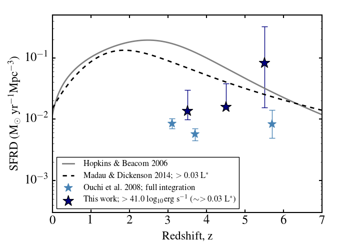
Figure 9: Contribution of LAEs to the cosmic SFRD in our three redshift bins at $2.91\leq z<4.00$ $4.00\leq z<5.00$, and $5.00\leq z<6.64$ integrating to log₁₀ L${}^{*}=41.0$ ($0.02$ L^∗ in the lower two redshift bins, and $0.03$ L^∗ in our highest redshift bin). The lighter blue stars show the results of Ouchi et al. (2008) for a full integration of the Ly$\alpha$ luminosity function. The LAE results are compared to literature studies of continuum-selected galaxies traced by the solid and dashed lines. We find that LAEs’ contribution to the SFRD rises towards higher redshift, although their contribution relative to that of more massive galaxies is uncertain due to various limitations (e.g. inhomogeneous integration limits from many different surveys, and the uncertainty in translating Ly$\alpha$ luminosity density to an SFRD).

To determine our Ly$\alpha$ luminosity densities we integrate the maximum likelihood luminosity function in each of our redshift bins to log₁₀ L${}^{*}=41.0$ ($0.02$ L^∗ in the lower two redshift bins, and $0.03$ L^∗ in our highest redshift bin, shown in the penultimate column of Table 1). We make the assumption that the entirety of the Ly$\alpha$ emission is produced by star-formation, and use Equation 7:

$${{\rm{SFR}_{Ly\alpha}}{\rm{M_{\odot}}}{\rm{yr}}^{-1}{\rm{Mpc}}^{-3}={\rm{L}_{Ly\alpha}ergs}^{-1}/1.05\times 10.0^{42.0},}$$ (7)

as in Ouchi et al. (2008), to convert the Ly$\alpha$ luminosity density to an SFRD. We note that this is a very uncertain conversion, however we show in Figure 9 our best estimates of the LAE SFRD derived from the Ly$\alpha$ line, over-plotted on two parameterisations of the global SFRD from $z=7$ to the present day (from Hopkins & Beacom 2006 and Madau & Dickinson 2014 which compile estimates from rest-frame UV through to radio). These studies also faced of course the question of where to place the integration limit for luminosity functions drawn from the literature. Madau & Dickinson (2014) for example chose to use a cutoff at $0.03$ L^∗ across all wavelengths in an attempt to homogenise the data. The limit is comparable to our own, however we note that by changing the integration limit of either our own luminosity functions, or those from the literature, one could draw very different conclusions as to the fraction of the total SFRD that LAEs are contributing.

Ouchi et al. (2008) used $858$ narrowband selected LAEs to estimate the SFRD in three redshift slices at $z=3.1,3.7$ and $5.7$ assuming a Ly$\alpha$ escape fraction $=1$ (shown in Figure 9 by the light blue stars). They concluded that on average LAEs contribute $\approx 20\%$ to $\approx 40\%$ of the SFRD from broadband selected surveys over the entire period.

Similarly, Cassata et al. (2011) used the VVDS spectroscopic survey to make the same measurement using Ly$\alpha$ LFs (with luminosities offset from their observed values according to the IGM attenution prescription of Fan et al. 2006). With this approach they compared the contribution of LAEs to the SFRD as measured from LBG surveys. Only a fraction of LBGs are also LAEs (when LAEs are defined to have a Ly$\alpha$ equivalent width greater than some cutoff) and the fraction of LAEs amongst LBGs is known to increase towards fainter UV magnitudes. With MUSE we probe a population of galaxies that are fainter than average in the UV, in contrast to the majority of objects defined as LBGs. As such, it is difficult to state what fraction of the overall SFRD LAEs contribute. Cassata et al. (2011) found that the LAE-derived SFRD increases from $\approx 20\%$ at $z\approx 2.5$ to $\approx 100\%$ by $z\approx 6.0$ relative to LBG estimates. We find very similar results from our observed luminosity functions. In our lowest redshift bin LAEs contribute $10$ - $20\%$ of the SFRD depending on whether one compares to the Madau & Dickinson (2014) or Hopkins & Beacom (2006) parameterisations, reaching $100\%$ by redshift $z\approx 6.0$. In fact our best estimate of the SFRD at this redshift is actually greater than the estimates from other star-formation tracers, probably indicating the inadequacies of making a direct transformation from Ly$\alpha$ luminosity to a star-formation rate in addition to the very different sample selections (the majority of previous surveys trace massive continuum-bright sources). It would appear that the steep values of $\alpha$ we measure, and the steepening of the slope with increasing redshift easily allow the resultant SFRD to match or even exceed estimates from broadband selected galaxies. This means that any further boost in the luminosity density (such as from introducing an IGM attenuation correction) would act to raise LAEs’ contribution to the broadband selected SFRD further, such that LAEs may play a more significant role in powering the early Universe than first thought.

This result is not a huge surprise, as we know that the steeper the luminosity function, the more dramatically the Ly$\alpha$ luminosity density (and hence the SFRD) increases for a given integration limit (also discussed in section 7.3 of Drake et al. 2013). Thus, it follows that our highest redshift luminosity function produces a significantly greater SFRD when integrated to the same limit as the two lower redshift bins, largely driven by the steep values of $\alpha$ we measure. Indeed, this behaviour of the integrated luminosity function is one of the drivers of the need to accurately measure the value of $\alpha$ for the high redshift population.

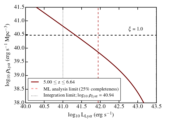
Figure 10: Integrating the maximum likelihood Schechter function at ($5.00\leq z<6.64$) to log L = 41.0 produces enough ionising radiation to maintain an ionised IGM at $z\approx 6$ for the set off assumptions described in the text.

6.3 Ly$\alpha$ luminosity density and implications for reionisation

In fact, it is the available ionising luminosity density which is the deciding factor in whether a given population were able to maintain an ionised IGM. As such, some groups have attempted to compute the critical Ly$\alpha$ luminosity that would translate to a sufficient ionising flux to maintain a transparent IGM. To place any constraint on this value at all, it is necessary to make various assumptions about the escape of Ly$\alpha$, the escape of Lyman continuum (LyC) and the clumping of the IGM.

We follow the arguments laid out in Martin et al. 2008 (also Dressler et al. 2011, Henry et al. 2012, Dressler et al. 2015), who take fiducial values of Ly$\alpha$ escape ($f_{esc}^{Ly\alpha}=0.5$; Martin et al. 2008), escape of LyC ($f_{esc}^{LyC}=0.1$; Chen et al. 2007, Shapley et al. 2006) and the clumping of the IGM ($C=6$; Madau et al. 1999) to determine a critical value of log₁₀ $\rho_{{\rm{\,Ly}}\alpha}=40.48$ erg s^-1 Mpc^-3 at $z=5.7$ (equation 5 of Martin et al. 2008):

$$\rho_{{\rm{Ly}}\alpha}=3.0\times 10^{40}{\rm{erg\,s}}^{-1}{\rm{Mpc^{-3}}}\times\,C_{6}(1-0.1f_{{{\rm{Lyc}},0.1}})$$

$$\left(\frac{f_{{{\rm{Ly}}\alpha},0.5}}{f_{{{\rm{Lyc}},0.1}}}\right)\left(\frac{1+z}{6.7}\right)^{3}\left(\frac{\Omega_{\,\beta}\,h^{2}_{\,70}}{0.047}\right)^{2}.$$ (8)

In Figure 10 we show the cumulative Ly$\alpha$ luminosity density, $\rho_{Ly\alpha}$ on the ordinate, against the limit of integration on the abscissa. Using our Schechter luminosity function at redshift ($5.00\leq z<6.64$) we integrate the most likely Schechter parameters down to log $L=41.0$ resulting in $\rho_{Ly\alpha}=40.94$.

We need only extrapolate by $<1$ dex beyond the $25\%$ completeness limit (the lowest luminosity galaxies included in the maximum likelihood analysis) in order to achieve a great enough $\rho_{Ly\alpha}$ to maintain reionisation, assuming our assumptions are valid.

7 Conclusions

We have presented a large, homogeneously-selected sample of $604$ LAEs in total from the MUSE-GTO observations of the HUDF. Using automatic detection software we build samples of $123$ and $481$ LAEs in the udf-10 and UDF-mosaic fields respectively. We simulate realistic extended LAEs based on the halo measurements of Wisotzki et al. (2016) and L17 to derive a fully-characterised LAE selection function for the Ly$\alpha$ luminosity function. As such we compute the deepest-ever Ly$\alpha$ luminosity function in a blank-field, taking into account extended Ly$\alpha$ emission, and using two different estimators to reduce the biases of a single approach. Our main findings can be summarised as follows:

• We find a steep faint-end slope of the Ly$\alpha$ luminosity function in each of our redshift bins using both the $1/$V_max- and maximum-likelihood estimators.

• We see no evidence of a strong evolution in the observed luminosity functions between our three $68\%$ confidence regions for L^∗-$\alpha$ in redshift bins at $2.91\leq z<4.00$ $4.00\leq z<5.00$, and $5.00\leq z<6.64$.

• Examining the faint-end slope $\alpha$ alone, we find an increase in the steepness of the luminosity function with increasing redshift.

• LAEs contribute significantly to the cosmic SFRD, reaching $100\%$ of that coming from continuum-selected LBG galaxies by redshift $z\approx 6.0$, using the very similar integration limits and the Ly$\alpha$ line flux to trace star formation activity. The increase is partly driven by the very steep faint-end slope at ($5.00\leq z<6.64$).

• LAEs undoubtedly produce a large fraction of the ionising radiation required to maintain a transparent IGM at $z\approx 6.0$. Taking fiducial values of several key factors, the maximum likelihood luminosity function requires only a small extrapolation beyond the data ($0.8$ dex) for LAEs alone to power reionisation.
  

The ability of MUSE to capture extended Ly$\alpha$ emission around individual high-redshift galaxies is transforming our view of the early Universe. Now that we are an order of magnitude more sensitive to Ly$\alpha$ line fluxes we find that faint LAEs were even more abundant in the early Universe than previously thought. In the near future, systematic surveys of Ly$\alpha$ line profiles from MUSE will allow us to select galaxies which are likely to be leaking LyC radiation, and in conjunction with simulations this will lead to a better understanding of the way that LAEs were able to power the reionisation of the IGM.

Appendix A Vmax results

Table 2: Differential Ly$\alpha$ luminosity function in bins of $\Delta$ log10 L= 0.4 using the $1/V_{max}$ estimator. Errors quoted on values of $\phi$ are $1\sigma$ assuming Poissonian statistics.

Redshift Bin (2.92 $\leq z<$ 4.00)
Bin log10 ($L$) [erg s-1]	log10 $L$median [ergs-1]	$\phi$ [(dlog10 $L$)-1 Mpc-3]	No. objects
$41.00<{\bf{41.200}}<41.40$	$41.309$	$0.02086\pm 0.00467$	$20$
$41.40<{\bf{41.600}}<41.80$	$41.633$	$0.03846\pm 0.00351$	$120$
$41.80<{\bf{42.000}}<42.20$	$41.967$	$0.01125\pm 0.00129$	$76$
$42.20<{\bf{42.400}}<42.60$	$42.316$	$0.00374\pm 0.00082$	$21$
$42.60<{\bf{42.800}}<43.00$	$42.807$	$0.00013\pm 0.00009$	$2$
Redshift Bin (4.00 $\leq z<$ 5.00)
Bin log10 ($L$) [erg s-1]	log10 $L$median [ergs-1]	$\phi$ [(dlog10 $L$)-1 Mpc-3]	No. objects
$41.00<{\bf{41.200}}<41.40$	$41.301$	$0.01871\pm 0.00454$	$17$
$41.40<{\bf{41.600}}<41.80$	$41.660$	$0.02489\pm 0.00284$	$77$
$41.80<{\bf{42.000}}<42.20$	$41.968$	$0.01137\pm 0.00138$	$68$
$42.20<{\bf{42.400}}<42.60$	$42.375$	$0.00249\pm 0.00052$	$23$
$42.60<{\bf{42.800}}<43.00$	$42.785$	$0.00145\pm 0.00065$	$5$
$43.00<{\bf{43.200}}<43.40$	$43.071$	$0.00008\pm 0.00008$	$1$
Redshift Bin (5.00 $\leq z<$ 6.64)
Bin log10 ($L$) [erg s-1]	log10 $L$median [ergs-1]	$\phi$ [(dlog10 $L$)-1 Mpc-3]	No. objects
$41.00<{\bf{41.200}}<41.40$	$41.235$	$0.0049\pm 0.0028$	$3$
$41.40<{\bf{41.600}}<41.80$	$41.664$	$0.0077\pm 0.0016$	$22$
$41.80<{\bf{42.000}}<42.20$	$42.000$	$0.0073\pm 0.0012$	$36$
$42.20<{\bf{42.400}}<42.60$	$42.321$	$0.0034\pm 0.0007$	$26$
$42.60<{\bf{42.800}}<43.00$	$42.744$	$0.0008\pm 0.0003$	$7$
$43.00<{\bf{43.200}}<43.40$	$43.194$	$0.0001\pm 0.0001$	$1$
Global Sample, Redshift (2.92 $\leq z<$ 6.64)
Bin log10 ($L$) [erg s-1]	log10 $L$median [ergs-1]	$\phi$ [(dlog10 $L$)-1 Mpc-3]	No. objects
$41.00<{\bf{41.200}}<41.40$	$41.303$	$0.02679\pm 0.00424$	$40$
$41.40<{\bf{41.600}}<41.80$	$41.643$	$0.03773\pm 0.00255$	$219$
$41.80<{\bf{42.000}}<42.20$	$41.971$	$0.01377\pm 0.00103$	$180$
$42.20<{\bf{42.400}}<42.60$	$42.333$	$0.00385\pm 0.00046$	$70$
$42.60<{\bf{42.800}}<43.00$	$42.766$	$0.00079\pm 0.00021$	$14$
$43.00<{\bf{43.200}}<43.40$	$43.133$	$0.00004\pm 0.00003$	$2$