Dispersion for Data-Driven Algorithm Design, Online Learning, and Private Optimization

Abstract

A crucial problem in modern data science is data-driven algorithm design, where the goal is to choose the best algorithm, or algorithm parameters, for a specific application domain. In practice, we often optimize over a parametric algorithm family, searching for parameters with high performance on a collection of typical problem instances. While effective in practice, these procedures generally have not come with provable guarantees. A recent line of work initiated by a seminal paper of Gupta and Roughgarden [34] analyzes application-specific algorithm selection from a theoretical perspective. We progress this research direction in several important settings. We provide upper and lower bounds on regret for algorithm selection in online settings, where problems arrive sequentially and we must choose parameters online. We also consider differentially private algorithm selection, where the goal is to find good parameters for a set of problems without divulging too much sensitive information contained therein.

We analyze several important parameterized families of algorithms, including SDP-rounding schemes for problems formulated as integer quadratic programs as well as greedy techniques for several canonical subset selection problems. The cost function that measures an algorithm’s performance is often a volatile piecewise Lipschitz function of its parameters, since a small change to the parameters can lead to a cascade of different decisions made by the algorithm. We present general techniques for optimizing the sum or average of piecewise Lipschitz functions when the underlying functions satisfy a sufficient and general condition called dispersion. Intuitively, a set of piecewise Lipschitz functions is dispersed if no small region contains many of the functions’ discontinuities.

Using dispersion, we improve over the best-known online learning regret bounds for a variety problems, prove regret bounds for problems not previously studied, and provide matching regret lower bounds. In the private optimization setting, we show how to optimize performance while preserving privacy for several important problems, providing matching upper and lower bounds on performance loss due to privacy preservation. Though algorithm selection is our primary motivation, we believe the notion of dispersion may be of independent interest. Therefore, we present our results for the more general problem of optimizing piecewise Lipschitz functions. Finally, we uncover dispersion in domains beyond algorithm selection, namely, auction design and pricing, providing online and privacy guarantees for these problems as well.

1 Introduction

Data-driven algorithm design, that is, choosing the best algorithm for a specific application, is a critical problem in modern data science and algorithm design. Rather than use off-the-shelf algorithms with only worst-case guarantees, a practitioner will often optimize over a family of parametrized algorithms, tuning the algorithm’s parameters based on typical problems from his domain. Ideally, the resulting algorithm will have high performance on future problems, but these procedures have historically come with no guarantees. In a seminal work, Gupta and Roughgarden [34] study algorithm selection in a distributional learning setting. Modeling an application domain as a distribution over typical problems, they show that a bound on the intrinsic complexity of the algorithm family prescribes the number of samples sufficient to ensure that any algorithm’s empirical and expected performance are close.

We advance the foundations of algorithm selection in several important directions: online and private algorithm selection. In the online setting, problem instances arrive one-by-one, perhaps adversarially. The goal is to select parameters for each instance in order to minimize regret, which is the difference between the cumulative performance of those parameters and the optimal parameters in hindsight. We also study private algorithm selection, where the goal is to find high-performing parameters over a set of problems without revealing sensitive information contained therein. Preserving privacy is crucial when problems depend on individuals’ medical or purchase data, for example.

We analyze several important, infinite families of parameterized algorithms. These include greedy techniques for canonical subset selection problems such as the knapsack and maximum weight independent set problems. We also study SDP-rounding schemes for problems that can be formulated as integer quadratic programs, such as max-cut, max-2sat, and correlation clustering. In these cases, our goal is to optimize, online or privately, the utility function that measures an algorithm’s performance as a function of its parameters, such as the value of the items added to the knapsack by a parameterized knapsack algorithm. The key challenge is the volatility of this function: a small tweak to the algorithm’s parameters can cause a cascade of changes in the algorithm’s behavior. For example, greedy algorithms typically build a solution by iteratively adding items that maximize a scoring rule. Prior work has proposed parameterizing these scoring rules and tuning the parameter to obtain the best performance for a given application [34]. Slightly adjusting the parameter can cause the algorithm to select items in a completely different order, potentially causing a sharp change in the quality of the selected items.

Despite this challenge, we show that in many cases, these utility functions are well-behaved in several respects and thus can be optimized online and privately. Specifically, these functions are piecewise Lipschitz and moreover, they satisfy a condition we call dispersion. Roughly speaking, a collection of piecewise Lipschitz functions is dispersed if no small region of space contains discontinuities for many of the functions. We provide general techniques for online and private optimization of the sum or average of dispersed piecewise Lipschitz functions. Taking advantage of dispersion in online learning, we improve over the best-known regret bounds for a variety problems, prove regret bounds for problems not previously studied, and provide matching regret lower bounds. In the privacy setting, we show how to optimize performance while preserving privacy for several important problems, giving matching upper and lower bounds on performance loss due to privacy.

Though our main motivation is algorithm selection, we expect dispersion is even more widely applicable, opening up an exciting research direction. For this reason, we present our main results more generally for optimizing piecewise Lipschitz functions. We also uncover dispersion in domains beyond algorithm selection, namely, auction design and pricing, so we prove online and privacy guarantees for these problems as well. Finally, we answer several open questions: Cohen-Addad and Kanade [17] asked how to optimize piecewise Lipschitz functions and Gupta and Roughgarden [34] asked which algorithm selection problems can be solved with no regret algorithms. As a bonus, we also show that dispersion implies generalization guarantees in the distributional setting. In this setting, the configuration procedure is given an iid sample of problem instances drawn from an unknown distribution $\mathcal{D}$, and the goal is to find the algorithm parameters with highest expected utility. By bounding the empirical Rademacher complexity, we show that the sample and expected utility for all algorithms in our class are close, implying that the optimal algorithm on the sample is approximately optimal in expectation.

1.1 Our contributions

In order to present our contributions, we briefly outline the notation we will use. Let $\mathcal{A}$ be an infinite set of algorithms parameterized by a set $\mathcal{C}\subseteq\mathbb{R}^{d}$. For example, $\mathcal{A}$ might be the set of knapsack greedy algorithms that add items to the knapsack in decreasing order of $v(i)/s(i)^{\rho}$, where $v(i)$ and $s(i)$ are the value and size of item $i$ and $\rho$ is a parameter. Next, let $\Pi$ be a set of problem instances for $\mathcal{A}$, such as knapsack problem instances, and let $u:\Pi\times\mathcal{C}\to[0,H]$ be a utility function where $u(x,\bm{\rho})$ measures the performance of the algorithm with parameters $\bm{\rho}$ on problem instance $x\in\Pi$. For example, $u(x,\rho)$ could be the value of the items chosen by the knapsack algorithm with parameter $\rho$ on input $x$.

We now summarize our main contributions. Since our results apply beyond application-specific algorithm selection, we describe them for the more general problem of optimizing piecewise Lipschitz functions.

Dispersion

Let $u_{1},\dots,u_{T}$ be a set of functions mapping a set $\mathcal{C}\subseteq\mathbb{R}^{d}$ to $[0,H]$. For example, in the application-specific algorithm selection setting, given a collection of problem instances $x_{1},\dots,x_{T}\in\Pi$ and a utility function $u:\Pi\times\mathcal{C}\to[0,H]$, each function $u_{i}(\cdot)$ might equal the function $u(x_{i},\cdot)$, measuring an algorithm’s performance on a fixed problem instance as a function of its parameters. Dispersion is a constraint on the functions $u_{1},\dots,u_{T}$. We assume that for each function $u_{i}$, we can partition $\mathcal{C}$ into sets $\mathcal{C}_{1},\dots,\mathcal{C}_{K}$ such that $u_{i}$ is $L$-Lipschitz on each piece, but $u_{i}$ may have discontinuities at the boundaries between pieces. In our applications, each set $\mathcal{C}_{i}$ is connected, but our general results hold for arbitrary sets. Informally, the functions $u_{1},\dots,u_{T}$ are $(w,k)$-dispersed if every Euclidean ball of radius $w$ contains discontinuities for at most $k$ of those functions (see Section 2 for a formal definition). This guarantees that although each function $u_{i}$ may have discontinuities, they do not concentrate in a small region of space. Dispersion is sufficient to prove strong learning generalization guarantees, online learning regret bounds, and private optimization bounds when optimizing the empirical utility $\frac{1}{T}\sum_{i=1}^{T}u_{i}$. In our applications, $w=T^{\alpha-1}$ and $k=\tilde{O}(T^{\alpha})$ with high probability for any $1/2\leq\alpha\leq 1$, ignoring problem-specific multiplicands.

Online learning

We prove that dispersion implies strong regret bounds in online learning, a fundamental area of machine learning [12]. In this setting, a sequence of functions $u_{1},\dots,u_{T}$ arrive one-by-one. At time $t$, the learning algorithm chooses a parameter vector $\bm{\rho}_{t}$ and then either observes the function $u_{t}$ in the full information setting or the scalar $u_{t}(\bm{\rho}_{t})$ in the bandit setting. The goal is to minimize expected regret: $\mathop{\mathbb{E}}[\max_{\bm{\rho}\in\mathcal{C}}\sum u_{t}(\bm{\rho})-u_{t}(\bm{\rho}_{t})]$. Under full information, we show that the exponentially-weighted forecaster [12] has regret bounded by $\tilde{O}(H(\sqrt{Td}+k)+TLw)$. When $w=1/\sqrt{T}$ and $k=\tilde{O}(\sqrt{T})$, this results in $\tilde{O}(\sqrt{T}(H\sqrt{d}+L))$ regret. We also prove a matching lower bound. This algorithm also preserves $(\epsilon,\delta)$-differential privacy with regret bounded by $\tilde{O}(H(\sqrt{T}d/\epsilon+k+\delta)+TLw)$. Finally, under bandit feedback, we show that a discretization-based algorithm achieves regret at most $\tilde{O}(H(\sqrt{dT(3R/w)^{d}}+k)+TLw)$. When $w=T^{-1/(d+2)}$ and $k=\tilde{O}(T^{(d+1)/(d+2)})$, this gives a bound of $\tilde{O}(T^{(d+1)/(d+2)}(H\sqrt{d(3R)^{d}}+L))$, matching the dependence on $T$ of a lower bound by Kleinberg et al. [39] for (globally) Lipschitz functions.

Online algorithm selection is generally not possible: Gupta and Roughgarden [34] give an algorithm selection problem for which no online algorithm can achieve sub-linear regret. Therefore, additional structure is necessary to prove guarantees, which we characterize using dispersion.

Private batch optimization

We demonstrate that it is possible to optimize over a set of dispersed functions while preserving differential privacy [24]. In this setting, the goal is to find the parameter $\bm{\rho}$ that maximizes average utility on a set $\mathcal{S}=\{u_{1},\dots,u_{T}\}$ of functions $u_{i}:\mathcal{C}\to\mathbb{R}$ without divulging much information about any single function $u_{i}$. Providing privacy at the granularity of functions is suitable when each function encodes sensitive information about one or a small group of individuals and each individual’s information is used to define only a small number of functions. For example, in the case of auction design and pricing problems, each function $u_{i}$ is defined by a set of buyers’ bids or valuations for a set of items. If a single buyer’s information is only encoded by a single function, then we preserve her privacy by not revealing sensitive information about any one function $u_{i}$. This will be the case, for example, if the buyers do not repeatedly return to buy the same items day after day. This is a common assumption in online auction design and pricing [9, 10, 11, 14, 38, 53, 21] because it means the buyers will not be strategic, aiming to trick the algorithm into setting lower prices in the future.

Differential privacy requires that an algorithm is randomized and its output distribution is insensitive to changing a single point in the input data. Formally, two multi-sets $\mathcal{S}$ and $\mathcal{S}^{\prime}$ of $T$ functions are neighboring, denoted $\mathcal{S}\sim\mathcal{S}^{\prime}$, if $|\mathcal{S}\Delta\mathcal{S}^{\prime}|\leq 1$. A randomized algorithm $\mathcal{A}$ is $(\epsilon,\delta)$-differentially private if, for any neighboring multi-sets $\mathcal{S}\sim\mathcal{S}^{\prime}$ and set $\mathcal{O}$ of outcomes, $\operatorname*{Pr}(\mathcal{A}(\mathcal{S})\in\mathcal{O})\leq e^{\epsilon}\operatorname*{Pr}(\mathcal{A}(\mathcal{S}^{\prime})\in\mathcal{O})+\delta$. In our setting, the algorithm’s input is a set $\mathcal{S}$ of $T$ functions, and the output is a point $\bm{\rho}\in\mathcal{C}$ that approximately maximizes the average of those functions. We show that the exponential mechanism [43] outputs $\hat{\bm{\rho}}\in\mathcal{C}$ such that with high probability $\frac{1}{T}\sum_{i=1}^{T}u_{i}(\hat{\bm{\rho}})\geq\max_{\bm{\rho}\in\mathcal{C}}\frac{1}{T}\sum_{i=1}^{T}u_{i}(\bm{\rho})-\tilde{O}(\frac{H}{T}(\frac{d}{\epsilon}+k)+Lw)$ while preserving $(\epsilon,0)$-differential privacy. We also give a matching lower bound. Our private algorithms always preserve privacy, even when dispersion does not hold.

Computational efficiency

In our settings, the functions have additional structure that enables us to design efficient implementations of our algorithms: for one-dimensional problems, there is a closed-form expression for the integral of the piecewise Lipschitz functions on each piece and for multi-dimensional problems, the functions are piecewise concave. We leverage tools from high-dimensional geometry [7, 42] to efficiently implement the integration and sampling steps required by our algorithms. Our algorithms have running time linear in the number of pieces of the utility function and polynomial in all other parameters.

1.2 Dispersion in algorithm selection problems

Algorithm selection.

We study algorithm selection for integer quadratic programs (IQPs) of the form $\max_{\bm{z}\in\{\pm 1\}^{n}}\bm{z}^{\top}A\bm{z}$, where $A\in\mathbb{R}^{n\times n}$ for some $n$. Many classic NP-hard problems can be formulated as IQPs, including max-cut [29], max-2SAT [29], and correlation clustering [15]. Many IQP approximation algorithms are semidefinite programming (SDP) rounding schemes; they solve the SDP relaxation of the IQP and round the resulting vectors to binary values. We study two families of SDP rounding techniques: $s$-linear rounding [27] and outward rotation [61], which include the Goemans-Williamson algorithm [29] as a special case. Due to these algorithms’ inherent randomization, finding an optimal rounding function over $T$ problem instances with $n$ variables amounts to optimizing the sum of $(1/T^{1-\alpha},\tilde{O}(nT^{\alpha}))$-dispersed functions for $1/2\leq\alpha<1$. This holds even for adversarial (non-stochastic) instances, implying strong online learning guarantees.

We also study greedy algorithm selection for two canonical subset selection problems: the knapsack and maximum weight independent set (MWIS) problems. Greedy algorithms are typically defined by a scoring rule determining the order the algorithm adds elements to the solution set. For example, Gupta and Roughgarden [34] introduce a parameterized knapsack algorithm that adds items in decreasing order of $v(i)/s(i)^{\rho}$, where $v(i)$ and $s(i)$ are the value and size of item $i$. Under mild conditions — roughly, that the items’ values are drawn from distributions with bounded density functions and that each item’s size is independent from its value — we show that the utility functions induced by $T$ knapsack instances with $n$ items are $(1/T^{1-\alpha},\tilde{O}(nT^{\alpha}))$-dispersed for any $1/2\leq\alpha<1$.

Pricing problems and auction design

Market designers use machine learning to design auctions and set prices [60, 35]. In the online setting, at each time step there is a set of goods for sale and a set of consumers who place bids for those goods. The goal is to set auction parameters, such as reserve prices, that are nearly as good as the best fixed parameters in hindsight. Here, “best” may be defined in terms of revenue or social welfare, for example. In the offline setting, the algorithm receives a set of bidder valuations sampled from an unknown distribution and aims to find parameters that are nearly optimal in expectation (e.g., [26, 18, 36, 44, 46, 52, 20, 31, 11, 47, 3, 5]). We analyze multi-item, multi-bidder second price auctions with reserves, as well as pricing problems, where the algorithm sets prices and buyers decide what to buy based on their utility functions. These classic mechanisms have been studied for decades in both economics and computer science. We note that data-driven mechanism design problems are effectively algorithm design problems with incentive constraints: the input to a mechanism is the buyers’ bids or valuations, and the output is an allocation of the goods and a description of the payments required of the buyers. For ease of exposition, we discuss algorithm and mechanism design separately.

1.3 Related work

Gupta and Roughgarden [34] and Balcan et al. [4] study algorithm selection in the distributional learning setting, where there is a distribution $\mathcal{D}$ over problem instances. A learning algorithm receives a set $\mathcal{S}$ of samples from $\mathcal{D}$. Those two works provide uniform convergence guarantees, which bound the difference between the average performance over $\mathcal{S}$ of any algorithm in a class $\mathcal{A}$ and its expected performance on $\mathcal{D}$. It is known that regret bounds imply generalization guarantees for various online-to-batch conversion algorithms [13], but in this work, we also show that dispersion can be used to explicitly provide uniform convergence guarantees via Rademacher complexity. Beyond this connection, our work is a significant departure from these works since we give guarantees for private algorithm selection and we give no regret algorithms, whereas Gupta and Roughgarden [34] only study online MWIS algorithm selection, proving their algorithm has small constant per-round regret.

Private empirical risk minimization (ERM)

The goal of private ERM is to find the best machine learning model parameters based on private data. Techniques include objective and output perturbation [16], stochastic gradient descent, and the exponential mechanism [7]. These works focus on minimizing data-dependent convex functions, so parameters near the optimum also have high utility, which is not the case in our settings.

Private algorithm configuration

Kusner et al. [41] develop private Bayesian optimization techniques for tuning algorithm parameters. Their methods implicitly assume that the utility function is differentiable. Meanwhile, the class of functions we consider have discontinuities between pieces, and it is not enough to privately optimize on each piece, since the boundaries themselves are data-dependent.

Online optimization

Prior work on online algorithm selection focuses on significantly more restricted settings. Cohen-Addad and Kanade [17] study single-dimensional piecewise constant functions under a “smoothed adversary,” where the adversary chooses a distribution per boundary from which that boundary is drawn. Thus, the boundaries are independent. Moreover, each distribution must have bounded density. Gupta and Roughgarden [34] study online MWIS greedy algorithm selection under a smoothed adversary, where the adversary chooses a distribution per vertex from which its weight is drawn. Thus, the vertex weights are independent and again, each distribution must have bounded density. In contrast, we allow for more correlations among the elements of each problem instance. Our analysis also applies to the substantially more general setting of optimizing piecewise Lipschitz functions. We show several new applications of our techniques in algorithm selection for SDP rounding schemes, price setting, and auction design, none of which were covered by prior work. Furthermore, we provide differential privacy results and generalization guarantees.

Neither Cohen-Addad and Kanade [17] nor Gupta and Roughgarden [34] develop a general theory of dispersion, but we can map their analysis into our setting. In essence, Cohen-Addad and Kanade [17], who provide the tighter analysis, show that if the functions the algorithm sees map from $[0,1]$ to $[0,1]$ and are $(w,1)$-dispersed, then the regret of their algorithm is bounded by $O(\sqrt{T\ln(1/w)})$. Under a smoothed adversary, the functions are $(w,1)$-dispersed for an appropriate choice of $w$. In this work, we show that using the more general notion of $(w,k)$-dispersion is essential to proving tight learning bounds for more powerful adversaries. We provide a sequence of piecewise constant functions $u_{1},\dots,u_{T}$ mapping $[0,1]$ to $[0,1]$ that are $(1/8,\sqrt{T}+1)$-dispersed, which means that our regret bound is $O(\sqrt{T\log(1/w)}+k)=O(\sqrt{T})$. However, these functions are not $(w,1)$-disperse for any $w\geq 2^{-T}$, so the regret bound by Cohen-Addad and Kanade [17] is trivial, since $\sqrt{T\log(1/w)}$ with $w=2^{-T}$ equals $T$. Similarly, Weed et al. [59] and Feng et al. [28] use a notion similar to $(w,1)$-dispersion to prove learning guarantees for the specific problem of learning to bid, as do Rakhlin et al. [50] for learning threshold functions under a smoothed adversary.

Our online bandit results are related to those of Kleinberg [37] for the “continuum-armed bandit” problem. They consider bandit problems where the set of arms is the interval $[0,1]$ and each payout function is uniformly locally Lipschitz. We relax this requirement, allowing each payout function to be Lipschitz with a number of discontinuities. In exchange, we require that the overall sequence of payout functions is fairly nice, in the sense that their discontinuities do not tightly concentrate. The follow-up work on Multi-armed Bandits in Metric Spaces [39] considers the stochastic bandit problem where the space of arms is an arbitrary metric space and the mean payoff function is Lipschitz. They introduce the zooming algorithm, which has better regret bounds than the discretization approach of Kleinberg [37] when either the max-min covering dimension or the (payout-dependent) zooming dimension are smaller than the covering dimension. In contrast, we consider optimization over $\mathbb{R}^{d}$ under the $\ell_{2}$ metric, where this algorithm does not give improved regret in the worst case.

Auction design and pricing

Several works [9, 10, 11, 14, 38, 53] present stylized online learning algorithms for revenue maximization under specific auction classes. In contrast, our online algorithms are highly general and apply to many optimization problems beyond auction design. Dudík et al. [21] also provide online algorithms for auction design. They discretize each set of mechanisms they consider and prove their algorithms have low regret over the discretized set. When the bidders have simple valuations (unit-demand and single-parameter) minimizing regret over the discretized set amounts to minimizing regret over the entire mechanism class. In contrast, we study bidders with fully general valuations, as well as additive and unit-demand valuations.

A long line of work has studied generalization guarantees for auction design and pricing problems (e.g., [26, 18, 36, 44, 46, 52, 20, 31, 11, 47, 30, 3, 5]). These works study the distributional setting where there is an unknown distribution over buyers’ values and the goal is to use samples from this distribution to design a mechanism with high expected revenue. Generalization guarantees bound the difference between a mechanism’s empirical revenue over the set of samples and expected revenue over the distribution. For example, several of these works [44, 46, 47, 3, 5, 45, 56] use learning theoretic tools such as pseudo-dimension and Rademacher complexity to derive these generalization guarantees. In contrast, we study online and private mechanism design, which requires a distinct set of analysis tools beyond those used in the distributional setting.

Bubeck et al. [11] study auction design in both the online and distributional settings when there is a single item for sale. They take advantage of structure exhibited in this well-studied single-item setting, such as the precise form of the optimal single-item auction [48]. Meanwhile, our algorithms and guarantees apply to the more general problem of optimizing piecewise Lipschitz functions.

2 Dispersion condition

In this section we formally define $(w,k)$-dispersion using the same notation as in Section 1.1. Recall that $\Pi$ is a set of instances, $\mathcal{C}\subset\mathbb{R}^{d}$ is a parameter space, and $u$ is an abstract utility function. Throughout this paper, we use the $\ell_{2}$ distance and let $B(\bm{\rho},r)=\{\bm{\rho}^{\prime}\in\mathbb{R}^{d}\,:\,\|\bm{\rho}-\bm{\rho}^{\prime}\|_{2}\leq r\}$ denote a ball of radius $r$ centered at $\bm{\rho}$.

Definition 1.

Let $u_{1},\dots,u_{T}:\mathcal{C}\to[0,H]$ be a collection of functions where $u_{i}$ is piecewise Lipschitz over a partition $\mathcal{P}_{i}$ of $\mathcal{C}$. We say that $\mathcal{P}_{i}$ splits a set $A$ if $A$ intersects with at least two sets in $\mathcal{P}_{i}$ (see Figure 1). The collection of functions is $(w,k)$-dispersed if every ball of radius $w$ is split by at most $k$ of the partitions $\mathcal{P}_{1},\dots,\mathcal{P}_{T}$. More generally, the functions are $(w,k)$-dispersed at a maximizer if there exists a point $\bm{\rho}^{*}\in\operatorname*{argmax}_{\bm{\rho}\in\mathcal{C}}\sum_{i=1}^{T}u_{i}(\bm{\rho})$ such that the ball $B(\bm{\rho}^{*},w)$ is split by at most $k$ of the partitions $\mathcal{P}_{1},\dots,\mathcal{P}_{T}$.

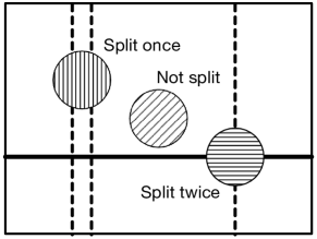
Figure 1: The dashed and solid lines correspond to two partitionings of the rectangle. Each of the displayed balls is either not split, split by one partition, or split by both.

Given $\mathcal{S}=\{x_{1},\dots,x_{T}\}\subseteq\Pi$ and a utility function $u:\Pi\times\mathcal{C}\to[0,H]$, we equivalently say that $u$ is $(w,k)$-dispersed for $\mathcal{S}$ (at a maximizer) if $\{u(x_{1},\cdot),\dots,u(x_{T},\cdot)\}$ is $(w,k)$-dispersed (at a maximizer).

We often show that the discontinuities of a piecewise Lipschitz function $u:\mathbb{R}\to\mathbb{R}$ are random variables with $\kappa$-bounded distributions. A density function $f:\mathbb{R}\to\mathbb{R}$ corresponds to a $\kappa$-bounded distribution if $\max\{f(x)\}\leq\kappa$. To prove dispersion we will use the following probabilistic lemma, showing that samples from $\kappa$-bounded distributions do not tightly concentrate.

Lemma 1.

Let $\mathcal{B}=\{\beta_{1},\dots,\beta_{r}\}\subset\mathbb{R}$ be a collection of samples where each $\beta_{i}$ is drawn from a $\kappa$-bounded distribution with density function $p_{i}$. For any $\zeta\geq 0$, the following statements hold with probability at least $1-\zeta$:

1. If the $\beta_{i}$ are independent, then every interval of width $w$ contains at most $k=O(rw\kappa+\sqrt{r\log(1/\zeta)})$ samples. In particular, for any $\alpha\geq 1/2$ we can take $w=1/(\kappa r^{1-\alpha})$ and $k=O(r^{\alpha}\sqrt{\log(1/\zeta)})$.

2. If the samples can be partitioned into $P$ buckets $\mathcal{B}_{1},\dots,\mathcal{B}_{P}$ such that each $\mathcal{B}_{i}$ contains independent samples and $|\mathcal{B}_{i}|\leq M$, then every interval of width $w$ contains at most $k=O(PMw\kappa+\sqrt{M\log(P/\zeta)}$. In particular, for any $\alpha\geq 1/2$ we can take $w=1/(\kappa M^{1-\alpha})$ and $k=O(PM^{\alpha}\sqrt{\log(P/\zeta)})$.

Proof sketch.

If the $\beta_{i}$ are independent, the expected number of samples in any interval of width $w$ is at most $r\kappa w$. Since the VC-dimension of intervals is 2, it follows that with probability at least $1-\zeta$, no interval contains more than $r\kappa w+O(\sqrt{r\log(1/\zeta)})$ samples.

The second claim follows by applying this counting argument to each of the buckets $\mathcal{B}_{i}$ with failure probability $\zeta^{\prime}=\zeta/P$ and taking the union bound over all buckets. With probability at least $1-\zeta$, every interval of width $w$ contains at most $M\kappa w+O(\sqrt{M\log(P/\zeta)})$ samples from each bucket, and at most $k=PM\kappa w+O(P\sqrt{M\log(P/\zeta)})$ samples in total from all $P$ buckets. ∎

Lemma 1 allows us to provide dispersion guarantees for “smoothed adversaries” in online learning. Under this type of adversary, the discontinuity locations for each function $u_{i}$ are random variables, due to the smoothness of the adversary. In our algorithm selection applications, the randomness of discontinuities may be a byproduct of the randomness in the algorithm’s inputs. For example, in the case of knapsack algorithm configuration, the item values and sizes may be drawn from distributions chosen by the adversary. This induces randomness in the discontinuity locations of the algorithm’s cost function. We can thus apply Lemma 1 to guarantee dispersion.

We also use Lemma 1 to guarantee dispersion even when the adversary is not smoothed. Surprisingly, we show that dispersion holds for IQP algorithm configuration without any assumptions on the input instances. In this case, we exploit the fact that the algorithms are themselves randomized. This randomness implies that the discontinuities of the algorithm’s cost function are random variables, and thus Lemma 1 implies dispersion.

3 Online optimization

In this setting, a sequence of functions $u_{1},\dots,u_{T}$ arrive one-by-one. At time $t$, the learning algorithm chooses a vector $\bm{\rho}_{t}$ and then either observes the function $u_{t}(\cdot)$ in the full information setting or the value $u_{t}(\bm{\rho}_{t})$ in the bandit setting. The goal is to minimize expected regret: $\mathop{\mathbb{E}}[\max_{\bm{\rho}\in\mathcal{C}}\sum_{t=1}^{T}(u_{t}(\bm{\rho})-u_{t}(\bm{\rho}_{t}))]$. In our applications, the functions $u_{1}$, …, $u_{T}$ are random, either due to internal randomization in the algorithms we are configuring or from assumptions on the adversary. We show that the functions are $(w,k)$-dispersed with probability $1-\zeta$ over the choice of $u_{1}$, …, $u_{T}$. The following regret bounds hold in expectation with an additional term of $HT\zeta$ bounding the effect of the rare event where the functions are not dispersed.

Full information. The exponentially-weighted forecaster algorithm samples the vectors $\bm{\rho}_{t}$ from the distribution $p_{t}(\bm{\rho})\propto\exp(\lambda\sum_{s=1}^{t-1}u_{s}(\bm{\rho}))$. We prove the following regret bound. The full proof is in Appendix C.

Theorem 1.

Let $u_{1},\dots,u_{T}:\mathcal{C}\to[0,H]$ be any sequence of piecewise $L$-Lipschitz functions that are $(w,k)$-dispersed at the maximizer $\bm{\rho}^{*}$. Suppose $\mathcal{C}\subset\mathbb{R}^{d}$ is contained in a ball of radius $R$ and $B(\bm{\rho^{*}},w)\subset\mathcal{C}$. The exponentially weighted forecaster with $\lambda=\sqrt{d\ln(R/w)/T}/H$ has expected regret bounded by

$$O\left(H\left(\sqrt{Td\log\frac{R}{w}}+k\right)+TLw\right).$$

For all rounds $t\in[T]$, suppose $\sum_{s=1}^{t}u_{s}$ is piecewise Lipschitz over at most $K$ pieces. When $d=1$ and $\exp(\sum_{s=1}^{t}u_{s})$ can be integrated in constant time on each of its pieces, the running time is $O(TK)$. When $d>1$ and $\sum_{s=1}^{t}u_{s}$ is piecewise concave over convex pieces, we provide an efficient approximate implementation. For approximation parameters $\eta=\zeta=1/\sqrt{T}$ and $\lambda=\sqrt{d\ln(R/w)/T}/H$, this algorithm has the same regret bound as the exact algorithm and runs in time $\tilde{O}(T(K\cdot\operatorname{poly}(d,1/\eta)+\operatorname{poly}(d,L,1/\eta)).$

Proof sketch.

Let $U_{t}$ be the function $\sum_{i=1}^{t-1}u_{i}(\cdot)$ and let $W_{t}=\int_{\mathcal{C}}\exp(\lambda U_{t}(\bm{\rho}))\,d\bm{\rho}$. We use $(w,k)$-dispersion to lower bound $W_{T+1}/W_{1}$ in terms of the optimal parameter’s total payout. Combining this with a standard upper bound on $W_{T+1}/W_{1}$ in terms of the learner’s expected payout gives the regret bound. To lower bound $W_{T+1}/W_{1}$, let $\bm{\rho}^{*}$ be the optimal parameter and let $\mathrm{OPT}=U_{T+1}(\bm{\rho}^{*})$. Also, let $\mathcal{B}^{*}$ be the ball of radius $w$ around $\bm{\rho}^{*}$. From $(w,k)$-dispersion, we know that for all $\bm{\rho}\in\mathcal{B}^{*}$, $U_{T+1}(\bm{\rho})\geq\mathrm{OPT}-Hk-LTw$. Therefore,

$$W_{T+1} =\int_{\mathcal{C}}\exp(\lambda U_{T+1}(\bm{\rho}))\,d\bm{\rho}\geq\int_{\mathcal{B}^{*}}\exp(\lambda U_{T+1}(\bm{\rho}))\,d\bm{\rho}$$

$$\geq\int_{\mathcal{B}^{*}}\exp(\lambda(\mathrm{OPT}-Hk-LTw))d\bm{\rho}$$

$$\geq\operatorname{Vol}(B(\bm{\rho}^{*},w))\exp(\lambda(\mathrm{OPT}-Hk-LTw)).$$

Moreover, $W_{1}=\int_{\mathcal{C}}\exp(\lambda U_{1}(\bm{\rho}))\,d\bm{\rho}\leq\operatorname{Vol}(B(\bm{0},R))$. Therefore,

$$\frac{W_{T+1}}{W_{1}}\geq\frac{\operatorname{Vol}(B(\bm{\rho}^{*},w))}{\operatorname{Vol}(B(\bm{0},R))}\exp(\lambda(\mathrm{OPT}-Hk-LTw)).$$

The volume ratio is equal to $(w/R)^{d}$, since the volume of a ball of radius $r$ in $\mathbb{R}^{d}$ is proportional to $r^{d}$. Therefore, $W_{T+1}/W_{1}\geq\left(w/R\right)^{d}\exp(\lambda(\mathrm{OPT}-Hk-LTw)).$ Combining the upper and lower bounds on $\frac{W_{T+1}}{W_{1}}$ gives the result.

Our efficient algorithm (Algorithm 4 of Appendix C) approximately samples from $p_{t}$. Let $\mathcal{C}_{1},\dots,\mathcal{C}_{K}$ be the partition of $\mathcal{C}$ over which $\sum u_{t}(\cdot)$ is piecewise concave. Our algorithm picks $\mathcal{C}_{I}$ with probability approximately proportional to $\int_{\mathcal{C}_{I}}p_{t}$ [42] and outputs a sample from the conditional distribution of $p_{t}$ on $\mathcal{C}_{I}$ [7]. Crucially, we prove that the algorithm’s output distribution is close to $p_{t}$, so every event concerning the outcome of the approximate algorithm occurs with about the same probability as it does under $p_{t}$. ∎

The requirement that $B(\bm{\rho^{*}},w)\subset\mathcal{C}$ is for convenience. In Lemma 12 of Appendix C we show how to transform the problem to satisfy this. Setting $\lambda=\sqrt{d/T}/H$, which does not require knowledge of $w$, has regret $O(H(\sqrt{Td}\log(R/w)+k)+TLw).$ Under alternative settings of $\lambda$, we show that our algorithms are $(\epsilon,\delta)$-differentially private with regret bounds of $\tilde{O}(H\sqrt{T}/\epsilon+Hk+LTw)$ in the single-dimensional setting and $\tilde{O}(H\sqrt{T}d/\epsilon+H(k+\delta)+LTw)$ in the $d$-dimensional setting (see Theorems 14 and 15 in Appendix C).

Next, we prove a matching lower bound. We warm up with a proof for the single-dimensional case in Appendix C.3 and then generalize that intuition to the multi-dimensional case in Appendix C.4.

Theorem 2.

Suppose $T\geq d$. For any algorithm, there are piecewise constant functions $u_{1},\dots,u_{T}$ mapping $[0,1]^{d}$ to $[0,1]$ such that if $D=\{(w,k):\{u_{1},\dots,u_{T}\}$ is $(w,k)$-dispersed at the maximizer$\},$ then

$$\max_{\bm{\rho}\in[0,1]^{d}}\mathop{\mathbb{E}}\left[\sum_{t=1}^{T}u_{t}\left(\bm{\rho}\right)-u_{t}\left(\bm{\rho}_{t}\right)\right]=\Omega\left(\inf_{(w,k)\in D}\left\{\sqrt{Td\log\frac{1}{w}}+k\right\}\right),$$

where the expectation is over the random choices $\bm{\rho}_{1},\dots,\bm{\rho}_{T}$ of the adversary.

Proof sketch.

For each dimension, the adversary plays a sequence of axis-aligned halfspaces with thresholds that divide the set of optimal parameters in two. The adversary plays each halfspace $\Theta(\frac{T}{d})$ times, randomly switching which side of the halfspace has a positive label, thus forcing regret of at least $\frac{\sqrt{Td}}{64}$. We prove that the resulting set of optimal parameters is contained in a hypercube of side length $\frac{1}{2}$. The adversary then plays $\sqrt{T}+d$ copies of the indicator function of a ball of radius $2^{-T}$ at the center of this cube. This ensures the functions are not $(w,0)$-dispersed at the maximizer for any $w\geq 2^{-T}$, and thus prior regret analyses [17] give a trivial bound of $T$. In order to prove the theorem, we need to show that $\frac{\sqrt{Td}}{64}=\Omega\left(\inf_{(w,k)\in D}\left\{\sqrt{Td\log\frac{1}{w}}+k\right\}\right)$. Therefore, we need to show that the set of functions played by the adversary is $(w,k)$-dispersed at the maximizer $\bm{\rho}^{*}$ for $w=\Theta(1)$ and $k=O\left(\sqrt{Td}\right).$ The reason this is true is that the only functions with discontinuities in the ball $\left\{\bm{\rho}:||\bm{\rho}^{*}-\bm{\rho}||\leq\frac{1}{8}\right\}$ are the final $\sqrt{T}+d$ functions played by the adversary. Thus, the theorem statement holds. ∎

Bandit feedback. We now study online optimization under bandit feedback.

Theorem 3.

Let $u_{1},\dots,u_{T}:\mathcal{C}\to[0,H]$ be any sequence of piecewise $L$-Lipschitz functions that are $(w,k)$-dispersed at the maximizer $\bm{\rho}^{*}$. Moreover, suppose that $\mathcal{C}\subset\mathbb{R}^{d}$ is contained in a ball of radius $R$ and that $B(\bm{\rho^{*}},w)\subset\mathcal{C}$. There is a bandit-feedback online optimization algorithm with regret

$$O\left(H\sqrt{Td\left(\frac{3R}{w}\right)^{d}\log\frac{R}{w}}+TLw+Hk\right).$$

The per-round running time is $O((3R/w)^{d})$.

Proof.

Let $\bm{\rho}_{1}$, …, $\bm{\rho}_{M}$ be a $w$-net for $\mathcal{C}$. The main insight is that $(w,k)$-dispersion implies that the difference in utility between the best point in hindsight from the net and the best point in hindsight from $\mathcal{C}$ is at most $Hk+TLw$. Therefore, we only need to compete with the best point in the net. We use the Exp3 algorithm [2] to choose parameters $\hat{\bm{\rho}}_{1}$, …, $\hat{\bm{\rho}}_{T}$ by playing the bandit with $M$ arms, where on round $t$ arm $i$ has payout $u_{t}(\bm{\rho}_{i})$. The expected regret of Exp3 is $\tilde{O}(H\sqrt{TM\log M})$ relative to our net. In Lemma 14 of Appendix C, we show $M\leq(3R/w)^{d}$, so the overall regret is $\tilde{O}(H\sqrt{Td(3R/w)^{d}\log(R/w)}+TLw+Hk)$ with respect to $\mathcal{C}$. ∎

If $w=T^{\frac{d+1}{d+2}-1}=\frac{1}{T^{1/(d+2)}}$ and $k=\tilde{O}\left(T^{\frac{d+1}{d+2}}\right)$, Theorem 3 gives the optimal exponent on $T$. Specifically, the regret is $\tilde{O}\left(T^{(d+1)/(d+2)}\left(H\sqrt{d(3R)^{d}}+L\right)\right)$, and no algorithm can have regret $O\left(T^{\gamma}\right)$ for $\gamma<(d+1)/(d+2)$ for the special case of (globally) Lispchitz functions [39].

4 Differentially private optimization

We show that the exponential mechanism, which is $(\epsilon,0)$-differentially private, has high utility when optimizing the mean of dispersed functions. In this setting, the algorithm is given a collection of functions $u_{1},\dots,u_{T}:\mathcal{C}\to[0,H]$, each of which depends on some sensitive information. In cases where each function $u_{i}$ encodes sensitive information about one or a small group of individuals and each individual is present in a small number of functions, we can give meaningful privacy guarantees by providing differential privacy for each function in the collection. We say that two sets of $T$ functions are neighboring if they differ on at most one function. Recall that the exponential mechanism outputs a sample from the distribution with density proportional to $f_{\rm exp}^{\epsilon}(\bm{\rho})=\exp\bigl{(}\frac{\epsilon}{2\Delta T}\sum_{i=1}^{T}u_{i}(\bm{\rho})\bigr{)}$, where $\Delta$ is the sensitivity of the average utility. Since the functions $u_{i}$ are bounded, the sensitivity of $\frac{1}{T}\sum_{i=1}^{T}u_{i}$ satisfies $\Delta\leq H/T$. The following theorem states our utility guarantee. The full proof is in Appendix D.

Theorem 4.

Let $u_{1},\dots,u_{T}:\mathcal{C}\to[0,H]$ be piecewise $L$-Lipschitz and $(w,k)$-dispersed at the maximizer $\bm{\rho}^{*}$, and suppose that $\mathcal{C}\subset\mathbb{R}^{d}$ is convex, contained in a ball of radius $R$, and $B(\bm{\rho}^{*},w)\subset\mathcal{C}$. For any $\epsilon>0$, with probability at least $1-\zeta$, the output $\hat{\bm{\rho}}$ of the exponential mechanism satisfies

$$\frac{1}{T}\sum_{i=1}^{T}u_{i}\left(\hat{\bm{\rho}}\right)\geq\frac{1}{T}\sum_{i=1}^{T}u_{i}\left(\bm{\rho}^{*}\right)-O\left(\frac{H}{T\epsilon}\left(d\log\frac{R}{w}+\log\frac{1}{\zeta}\right)+Lw+\frac{Hk}{T}\right).$$

When $d=1$, this algorithm is efficient, provided $f_{\rm exp}^{\epsilon}$ can be efficiently integrated on each piece of $\sum_{i}u_{i}$. For $d>1$ we also provide an efficient approximate sampling algorithm when $\sum_{i}u_{i}$ is piecewise concave defined on $K$ convex pieces. This algorithm preserves $(\epsilon,\delta)$-differential privacy for $\epsilon>0$, $\delta>0$ with the same utility guarantee (with $\zeta=\delta$). The running time of this algorithm is $\tilde{O}(K\cdot\operatorname{poly}(d,1/\epsilon)+\operatorname{poly}(d,L,1/\epsilon))$.

Proof sketch.

The exponential mechanism can fail to output a good parameter if there are drastically more bad parameters than good. The key insight is that due to dispersion, the set of good parameters is not too small. In particular, we know that every $\bm{\rho}\in B(\bm{\rho^{*}},w)$ has $\frac{1}{T}\sum_{i}u_{i}(\bm{\rho})\geq\frac{1}{T}\sum_{i}u_{i}(\bm{\rho}^{*})-\frac{Hk}{T}-Lw$ because at most $k$ of the functions $u_{i}$ for have discontinuities in $B(\bm{\rho^{*}},w)$ and the rest are $L$-Lipschitz.

In a bit more detail, for a constant $c$ fixed later on, the probability that a sample from $\mu_{\rm exp}$ lands in $E=\{\bm{\rho}\,:\,\frac{1}{T}\sum_{i}u_{i}(\bm{\rho})\leq c\}$ is $F/Z$, where $F=\int_{E}f_{\rm exp}$ and $Z=\int_{\mathcal{C}}f_{\rm exp}$. We know that $F\leq\exp\left(\frac{T\epsilon c}{2H}\right)\operatorname{Vol}(E)\leq\exp\left(\frac{T\epsilon c}{2H}\right)\operatorname{Vol}\bigl{(}B(0,R)\bigr{)},$ where the second inequality follows from the fact that a ball of radius $R$ contains the entire space $\mathcal{C}$. To lower bound $Z$, we use the fact that at most $k$ of the functions $u_{1},\dots,u_{T}$ have discontinuities in the ball $B(\bm{\rho^{*}},w)$ and the rest of the functions are $L$-Lipschitz. It follows that for any $\bm{\rho}\in B(\bm{\rho^{*}},w)$, we have $\frac{1}{T}\sum_{i}u_{i}(\bm{\rho})\geq\frac{1}{T}\sum_{i}u_{i}(\bm{\rho}^{*})-\frac{Hk}{|\mathcal{S}|}-Lw$. This is because each of the $k$ functions with boundaries can affect the average utility by at most $H/|T|$ and otherwise $\frac{1}{T}\sum_{i}u_{i}(\cdot)$ is $L$-Lipschitz. Since $B(\bm{\rho^{*}},w)\subset\mathcal{C}$, this gives $Z\geq\exp\bigl{(}\frac{T\epsilon}{2H}(\frac{1}{T}\sum_{i}u_{i}(\bm{\rho}^{*}))-\frac{Hk}{T}-Lw)\bigr{)}\operatorname{Vol}\bigl{(}B(\bm{\rho^{*}},w)\bigr{)}$.

Putting the bounds together, we have that $F/Z\leq\exp\bigl{(}\frac{T\epsilon}{2H}(c-\frac{1}{T}\sum_{i}u_{i}(\bm{\rho}^{*})+\frac{Hk}{T}+Lw\bigr{)}\cdot\frac{\operatorname{Vol}(B(0,R))}{\operatorname{Vol}(B(\bm{\rho^{*}},w))}$. The volume ratio is equal to $(R/w)^{d}$, since the volume of a ball of radius $r$ in $\mathbb{R}^{d}$ is proportional to $r^{d}$. Setting this bound to $\zeta$ and solving for $c$ gives the result.

Our efficient implementation (Algorithm 2 in Appendix D) relies on the same tools as our approximate implementation of the exponentially weighted forecaster. The main step is proving the distribution of $\hat{\bm{\rho}}$ is close to the distribution with density $f_{\rm exp}$. ∎

In Appendix H, we also give a discretization-based computationally inefficient algorithm in $d$ dimensions that satisfies $(\epsilon,0)$-differential privacy.

We can tune the value of $w$ to make the dependence on $L$ logarithmic: if $T\geq\frac{2Hd}{w\epsilon L}$, then with probability $1-\zeta$, $\frac{1}{T}\sum_{i}u_{i}(\hat{\bm{\rho}})\geq\frac{1}{T}\sum_{i}u_{i}(\bm{\rho}^{*})-O\left(\frac{Hd}{T\epsilon}\log\frac{L\epsilon RT}{Hd}+\frac{Hk}{T}+\frac{H}{T\epsilon}\log\frac{1}{\zeta}\right)$ (Corollary 5 in Appendix D).

Finally, we provide a matching lower bound. See Appendix D for the full proof. When $d=1$, we can instantiate these lower bounds using MWIS instances.

Theorem 5.

For every dimension $d\geq 1$, privacy parameter $\epsilon>0$, failure probability $\zeta>0$, $T\geq\frac{d}{\epsilon}(\frac{\ln 2}{2}-\ln\frac{1}{\zeta}))$ and $\epsilon$-differentially private optimization algorithm $\mathcal{A}$ that takes as input a collection of $T$ piecewise constant functions mapping $B(0,1)\subset\mathbb{R}^{d}$ to $[0,1]$ and outputs an approximate maximizer, there exists a multiset $\mathcal{S}$ of such functions so that with probability at least $1-\zeta$, the output $\hat{\bm{\rho}}$ of $\mathcal{A}(\mathcal{S})$ satisfies

$$\frac{1}{T}\sum_{u\in\mathcal{S}}u(\hat{\bm{\rho}})\leq\max_{\bm{\rho}\in B(0,1)}\frac{1}{T}\sum_{u\in\mathcal{S}}u(\bm{\rho})-\Omega\biggl{(}\inf_{(w,k)}\frac{d}{T\epsilon}\biggl{(}\ln\frac{1}{w}-\ln\frac{1}{\zeta}\biggr{)}+\frac{k}{T}\biggr{)},$$

where the infimum is taken over all $(w,k)$-dispersion at the maximizer parameters satisfied by $\mathcal{S}$.

Proof sketch.

We construct $M=2^{d}$ multi-sets of functions $\mathcal{S}_{1},\dots,\mathcal{S}_{M}$, each with $T$ piecewise constant functions. For every pair $\mathcal{S}_{i}$ and $\mathcal{S}_{j}$, $|\mathcal{S}_{i}\Delta\mathcal{S}_{j}|$ is small but the set $I_{\mathcal{S}_{i}}$ of parameters maximizing $\sum_{u\in\mathcal{S}_{i}}u(\bm{\rho})$ is disjoint from $I_{\mathcal{S}_{j}}$. Therefore, for every pair $\mathcal{S}_{i}$ and $\mathcal{S}_{j}$, the distributions $\mathcal{A}(\mathcal{S}_{i})$ and $\mathcal{A}(\mathcal{S}_{j})$ are similar, and since $I_{\mathcal{S}_{1}},\dots,I_{\mathcal{S}_{t}}$ are disjoint, this means that for some $\mathcal{S}_{i}$, with high probability, the output of $\mathcal{A}(\mathcal{S}_{i})\not\in I_{\mathcal{S}_{i}}$. The key challenge is constructing the sets $\mathcal{S}_{i}$ so that the suboptimality of any point not in $I_{\mathcal{S}_{i}}$ is $\frac{d}{T\epsilon}\log\frac{R}{w}+\frac{k}{T}$, where $w$ and $k$ are dispersion parameters for $\mathcal{S}_{i}$. We construct $\mathcal{S}_{i}$ so that this suboptimality is $\Theta(\frac{d}{T\epsilon})$, which gives the desired result if $w=\Theta(R)$ and $k=\Theta(\frac{d}{\epsilon})$. To achieve these conditions, we carefully fill each $\mathcal{S}_{i}$ with indicator functions of balls centered packed in the unit ball $B(0,1)$. ∎

5 Dispersion in application-specific algorithm selection

We now analyze dispersion for a range of algorithm configuration problems. In the private setting, the algorithm receives samples $\mathcal{S}\sim\mathcal{D}^{T}$, where $\mathcal{D}$ is an arbitrary distribution over problem instances $\Pi$. The goal is to privately find a value $\hat{\bm{\rho}}$ that nearly maximizes $\sum_{x\in\mathcal{S}}u(x,\bm{\rho})$. In our applications, prior work [47, 34, 4] shows that $\hat{\bm{\rho}}$ nearly maximizes $\mathop{\mathbb{E}}_{x\sim\mathcal{D}}[u(x,\bm{\rho})]$. In the online setting, the goal is to find a value $\bm{\rho}$ that is nearly optimal in hindsight over a stream $x_{1},\dots,x_{T}$ of instances, or equivalently, over a stream $u_{1}=u(x_{1},\cdot),\dots,u_{T}=u(x_{T},\cdot)$ of functions. Each $x_{t}$ is drawn from a distribution $\mathcal{D}^{(t)}$, which may be adversarial. Thus in both settings, $\{x_{1},\dots,x_{T}\}\sim\mathcal{D}^{(1)}\times\cdots\times\mathcal{D}^{(T)}$, but in the private setting, $\mathcal{D}^{(1)}=\cdots=\mathcal{D}^{(T)}$.

Greedy algorithms. We study greedy algorithm configuration for two important problems: the maximum weight independent set (MWIS) and knapsack problems. In MWIS, there is a graph and a weight $w\left(v\right)\in\mathbb{R}_{\geq 0}$ for each vertex $v$. The goal is to find a set of non-adjacent vertices with maximum weight. The classic greedy algorithm repeatedly adds a vertex $v$ which maximizes $w\left(v\right)/\left(1+\deg\left(v\right)\right)$ to the independent set and deletes $v$ and its neighbors from the graph. Gupta and Roughgarden [34] propose the greedy heuristic $w\left(v\right)/\left(1+\deg\left(v\right)\right)^{\rho}$ where $\rho\in\mathcal{C}=[0,B]$ for some $B\in\mathbb{R}$. When $\rho=1$, the approximation ratio is $1/D$, where $D$ is the graph’s maximum degree [54]. We represent a graph as a tuple $\left(\bm{w},\bm{e}\right)\in\mathbb{R}^{n}\times\left\{0,1\right\}^{{n\choose 2}}$, ordering the vertices $v_{1},\dots,v_{n}$ in a fixed but arbitrary way. The function $u\left(\bm{w},\bm{e},\cdot\right)$ maps a parameter $\rho$ to the weight of the vertices in the set returned by the algorithm parameterized by $\rho$.

Theorem 6.

Suppose all vertex weights are in $(0,1]$ and for each $\mathcal{D}^{(i)}$, every pair of vertex weights has a $\kappa$-bounded joint distribution. For any $\bm{w}$ and $\bm{e}$, $u\left(\bm{w},\bm{e},\cdot\right)$ is piecewise 0-Lipschitz and for any $\alpha\geq 1/2$, with probability $1-\zeta$ over $\mathcal{S}\sim\bigtimes_{i=1}^{T}\mathcal{D}^{(i)}$, $u$ is

$$\left(\frac{1}{T^{1-\alpha}\kappa\ln n},O\left(n^{4}T^{\alpha}\sqrt{\ln\frac{n}{\zeta}}\right)\right)\text{-dispersed}$$

with respect to $\mathcal{S}$.

Proof sketch.

The utility $u\left(\bm{w}^{\left(t\right)},\bm{e}^{\left(t\right)},\rho\right)$ has a discontinuity when the ordering of two vertices under the greedy score swaps. Thus, the discontinuities have the form

$$\frac{\ln\left(w_{i}^{\left(t\right)}\right)-\ln\left(w_{j}^{\left(t\right)}\right)}{\ln\left(d_{1}\right)-\ln\left(d_{2}\right)}$$

for all $t\in[T]$ and $i,j,d_{1},d_{2}\in[n]$, where $w_{j}^{\left(t\right)}$ is the weight of the $j^{th}$ vertex of $\left(\bm{w}^{\left(t\right)},\bm{e}^{\left(t\right)}\right)$ [33]. We show that when pairs of vertex weights have $\kappa$-bounded joint distributions, then the discontinuities each have $\left(\kappa\ln n\right)$-bounded distributions. Let $\mathcal{B}_{i,j,d_{1},d_{2}}$ be the set of discontinuities contributed by vertices $i$ and $j$ with degrees $d_{1}$ and $d_{2}$ across all instances in $\mathcal{S}$. The buckets $\mathcal{B}_{i,j,d_{1},d_{2}}$ partition the discontinuities into $n^{4}$ sets of independent random variables. Therefore, applying Lemma 1 with $P=n^{4}$ and $M=T$ proves the claim. ∎

In Appendix E, we prove Theorem 6 and demonstrate that it implies strong optimization guarantees. The analysis for the knapsack problem is similar (see Appendix E.2).

Integer quadratic programming (IQP) algorithms. We now apply our dispersion analysis to two popular IQP approximation algorithms: $s$-linear [27] and outward rotation rounding algorithms [61]. The goal is to maximize a function $\sum_{i,j\in[n]}a_{ij}z_{i}z_{j}$ over $\bm{z}\in\left\{\pm 1\right\}^{n}$, where the matrix $A=\left(a_{ij}\right)$ has non-negative diagonal entries. Both algorithms are generalizations of the Goemans-Williamson (GW) max-cut algorithm [29]. They first solve the SDP relaxation $\sum_{i,j\in[n]}a_{ij}\langle\bm{u}_{i},\bm{u}_{j}\rangle$ subject to the constraint that $\|\bm{u}_{i}\|=1$ for $i\in[n]$ and then round the vectors $\bm{u}_{i}$ to $\left\{\pm 1\right\}$. Under $s$-linear rounding, the algorithm samples a standard Gaussian $\bm{Z}\sim\mathcal{N}_{n}$ and sets $z_{i}=1$ with probability $1/2+\phi_{s}\left(\langle\bm{u}_{i},\bm{Z}\rangle\right)/2$ and $-1$ otherwise, where $\phi_{s}\left(y\right)=-\mathbbm{1}_{y<-s}+\frac{y}{s}\cdot\mathbbm{1}_{-s\leq y\leq s}+\mathbbm{1}_{y>s}$ and $s$ is a parameter. The outward rotation algorithm first maps each $\bm{u}_{i}$ to $\bm{u}_{i}^{\prime}\in\mathbb{R}^{2n}$ by $\bm{u}_{i}^{\prime}=[\cos\left(\gamma\right)\bm{u}_{i}\,;\,\sin\left(\gamma\right)\bm{e}_{i}]$ and sets $z_{i}=\operatorname{sgn}\left(\langle\bm{u}_{i}^{\prime},\bm{Z}\rangle\right)$, where $\bm{e}_{i}$ is the $i^{\rm th}$ standard basis vector, $\bm{Z}\in\mathbb{R}^{2n}$ is a standard Gaussian, and $\gamma\in[0,\pi/2]$ is a parameter. Feige and Langberg [27] and Zwick [61] prove that these rounding functions provide a better worst-case approximation ratio on graphs with “light” max-cuts, where the max-cut does not constitute a large fraction of the edges.

Our utility $u$ maps the algorithm parameter (either $s$ or $\gamma$) to the objective value obtained. We exploit the randomness of these algorithms to guarantee dispersion. To facilitate this analysis, we imagine that the Gaussians $\bm{Z}$ are sampled ahead of time and included as part of the problem instance. For $s$-linear rounding, we write the utility as $u_{\rm slin}(A,\bm{Z},s)=\sum_{i=1}^{n}a_{i}^{2}+\sum_{i\not=j}a_{ij}\phi_{s}(v_{i})\phi_{s}(v_{j})$, where $v_{i}=\langle\bm{u_{i}},\bm{Z}\rangle$. For outward rotations, $u_{\rm owr}(A,\bm{Z},\gamma)=\sum_{i,j}a_{ij}\operatorname{sgn}(v^{\prime}_{i})\operatorname{sgn}(v^{\prime}_{j})$, where $v^{\prime}_{i}=\langle\bm{u}_{i}^{\prime},\bm{Z}\rangle$.

First, we prove a dispersion guarantee for $u_{\rm owr}$. The full proof is in Appendix E, where we also demonstrate the theorem’s implications for our optimization settings (Theorems 25, 26, 27, and 28).

Theorem 7.

For any matrix $A$ and vector $\bm{Z}$, $u_{\rm owr}\left(A,\bm{Z},\cdot\right)$ is piecewise $0$-Lipschitz. With probability $1-\zeta$ over $\bm{Z}^{\left(1\right)},\dots,\bm{Z}^{\left(T\right)}\sim\mathcal{N}_{2n}$, for any $A^{\left(1\right)},\dots,A^{\left(T\right)}\in\mathbb{R}^{n\times n}$ and any $\alpha\geq 1/2$, $u_{\rm owr}$ is

$$\left(T^{\alpha-1},O\left(nT^{\alpha}\sqrt{\log\frac{n}{\zeta}}\right)\right)\text{-dispersed}$$

with respect to $\mathcal{S}=\left\{\left(A^{\left(t\right)},\bm{Z}^{\left(t\right)}\right)\right\}_{t=1}^{T}$.

Proof sketch.

The discontinuities of $u_{\text{owr}}\left(A,\bm{Z},\gamma\right)$ occur whenever $\langle\bm{u}_{i}^{\prime},\bm{Z}\rangle$ shifts from positive to negative for some $i\in[n]$. Between discontinuities, the function is constant. By definition of $\bm{u}_{i}^{\prime}$, this happens when $\gamma=\tan^{-1}\left(-\langle\bm{u}_{i},\bm{Z}[1,\dots,n]\rangle/Z[n+i]\right)$, which comes from a $1/\pi$-bounded distribution. The next challenge is that the discontinuities are not independent: the $n$ discontinuities from instance $t$ depend on the same vector $\bm{Z}^{\left(t\right)}$. To overcome this, we let $\mathcal{B}_{i}$ denote the set of discontinuities contributed by vector $\bm{u}_{i}$ across all instances. The buckets $\mathcal{B}_{i}$ partition the set of discontinuities into $P=n$ sets, each containing at most $T$ discontinuities. We then apply Lemma 1 with $P$ and $M=T$ to prove the claim. ∎

Next, we prove the following guarantee for $u_{\rm slin}$. The full proof is in Appendix E, where we also demonstrate the theorem’s implications for our optimization settings (Theorems 29, 30, and 31).

Theorem 8.

With probability $1-\zeta$ over $\bm{Z}^{\left(1\right)},\dots,\bm{Z}^{\left(T\right)}\sim\mathcal{N}_{n}$, for any matrices $A^{\left(1\right)},\dots,A^{\left(T\right)}$ and any $\alpha\geq 1/2$, the functions $u_{\rm slin}\left(\bm{Z}^{\left(1\right)},A^{\left(1\right)},\cdot\right),\dots,u_{\rm slin}\left(\bm{Z}^{\left(T\right)},A^{\left(T\right)},\cdot\right)$ are piecewise $L$-Lipschitz with $L=\tilde{O}\left(MT^{3}n^{5}/\zeta^{3}\right)$, where $M=\max_{i,j\in[n],t\in[T]}|a_{ij}^{\left(t\right)}|$, and $u_{\rm slin}$ is

$$\left(T^{\alpha-1},O\left(nT^{\alpha}\sqrt{\log\frac{n}{\zeta}}\right)\right)\text{-dispersed}$$

with respect to $\mathcal{S}=\left\{\left(A^{\left(t\right)},\bm{Z}^{\left(t\right)}\right)\right\}_{t=1}^{T}$.

Proof sketch.

We show that over the randomness of $\bm{Z}^{\left(1\right)},\dots,\bm{Z}^{\left(T\right)}$, $u_{\text{slin}}$ is $\left(w,k\right)$-dispersed. By definition of $\phi_{s}$, the discontinuities of $u_{\text{slin}}\left(A^{\left(t\right)},\bm{Z}^{\left(t\right)},\cdot\right)$ have the form $s=|\langle\bm{u}_{i}^{\left(t\right)},\bm{Z}^{\left(t\right)}\rangle|$, where $\bm{u}_{i}^{\left(t\right)}$ is the $i^{\rm th}$ vector in the solution to SDP-relaxation of $A^{\left(t\right)}$. These random variables have density bounded by $\sqrt{2/\pi}$. Let $\mathcal{B}_{i}$ be the set of discontinuities contributed by $\bm{u}_{i}^{\left(1\right)},\dots,\bm{u}_{i}^{\left(T\right)}$. The points within each $\mathcal{B}_{i}$ are independent. We apply Lemma 1 with $P=n$ and $M=T$ and arrive at our dispersion guarantee.

Proving that the piecewise portions of $u_{\text{slin}}$ are Lipschitz is complicated by the fact that they are quadratic in $1/s$, so the slope may go to $\pm\infty$ as $s$ goes to 0. However, if $s$ is smaller than the smallest boundary $s_{0}$, $u_{\rm slin}\left(\bm{Z}^{\left(t\right)},A^{\left(t\right)},\cdot\right)$ is constant because $\phi_{s}$ deterministically maps the variables to $-1$ or 1, as in the GW algorithm. We prove that $s_{0}$ is not too small using anti-concentration bounds. The Lipschitz constant is then roughly bounded by $n^{2}/s_{0}^{3}$, since we take the derivative of the sum of $n^{2}$ inverse quadratic functions. ∎

6 Dispersion in pricing problems and auction design

In this section, we study $n$-bidder, $m$-item posted price mechanisms and second price auctions. We denote all $n$ buyers’ valuations for all $2^{m}$ bundles $b_{1},\dots,b_{2^{m}}\subseteq[m]$ by

$$\bm{v}=(v_{1}(b_{1}),\dots,v_{1}(b_{2^{m}}),\dots,v_{n}(b_{1}),\dots,v_{n}(b_{2^{m}})).$$

We study buyers with additive valuations $\left(v_{j}(b)=\sum_{i\in b}v_{j}(\{i\})\right)$ and unit-demand valuations ($v_{j}(b)=\max_{i\in b}v_{j}(\{i\})$). We also study buyers with general valuations, where there is no assumption on $v_{j}$ beyond the fact that it is nonnegative, monotone, and $v_{j}(\emptyset)=0$.

Posted price mechanisms are defined by $m$ prices $\rho_{1},\dots,\rho_{m}$ and a fixed ordering over the buyers. In order, each buyer has the option of buying her utility-maximizing bundle among the remaining items. In other words, suppose it is buyer $j$’s turn in the ordering and let $I$ be the set of items that buyers before her in the ordering did not buy. Then she will buy the bundle $b\subseteq I$ that maximizes $v_{j}(b)-\sum_{i\in b}\rho_{i}$.

Second price item auctions with anonymous reserve prices are defined by $m$ reserve prices $\rho_{1},\dots,\rho_{m}$. The bidders submit bids for each of the items. For each item $i$, the highest bidder wins the item if her bid is above $\rho_{i}$ and she pays the maximum of the second highest bid for item $i$ and $\rho_{i}$. These auctions are only strategy proof for additive bidders, which means that buyers have no incentive to misreport their values. Therefore, we restrict our attention to this setting and assume the bids equal the values.

In this setting, $\Pi$ is a set of valuation vectors $\bm{v}$ and as in Section 5, each $\mathcal{D}^{(t)}$ is a distribution over $\Pi$. The following results hold whenever the utility function corresponds to revenue (the sum of the payments) or social surplus (the sum of the buyers’ values for their allocations). The full proof is in Appendix F.

Theorem 9.

Suppose that $u(\bm{v},\bm{\rho})$ is the social welfare (respectively, revenue) of the posted price mechanism with prices $\bm{\rho}$ and buyers’ values $\bm{v}$. In this case, $L=0$ (respectively, $L=1$). The following are each true with probability at least $1-\zeta$ over the draw $\mathcal{S}\sim\mathcal{D}^{(1)}\times\cdots\times\mathcal{D}^{(T)}$ for any $\alpha\geq 1/2$:

1. Suppose the buyers have additive valuations and for each distribution $\mathcal{D}^{(t)}$, the item values have $\kappa$-bounded marginal distributions. Then $u$ is

   $$\left(\frac{1}{2\kappa T^{1-\alpha}},O\left(nmT^{\alpha}\sqrt{\ln\frac{nm}{\zeta}}\right)\right)\text{-dispersed}$$

   with respect to $\mathcal{S}$.

2. Suppose the buyers are unit-demand with $v_{j}(\{i\})\in[0,W]$ for each buyer $j\in[n]$ and item $i\in[m]$. Also, suppose that for each distribution $\mathcal{D}^{(t)}$, each buyer $j$, and every pair of items $i$ and $i^{\prime}$, $v_{j}(\{i\})$ and $v_{j}(\{i^{\prime}\})$ have a $\kappa$-bounded joint distribution. Then $u$ is

   $$\left(\frac{1}{2W\kappa T^{1-\alpha}},O\left(nm^{2}T^{\alpha}\sqrt{\ln\frac{nm}{\zeta}}\right)\right)\text{-dispersed}$$

   with respect to $\mathcal{S}$.

3. Suppose the buyers have general valuations in $[0,W]$. Also, suppose that for each $\mathcal{D}^{(t)}$, each buyer $j$, and every pair of bundles $b$ and $b^{\prime}$, $v_{j}(b)$ and $v_{j}(b^{\prime})$ have a $\kappa$-bounded joint distribution. Then $u$ is

   $$\left(\frac{1}{2W\kappa T^{1-\alpha}},O\left(n2^{2m}T^{\alpha}\sqrt{\ln\frac{n2^{m}}{\zeta}}\right)\right)\text{-dispersed}$$

   with respect to $\mathcal{S}$.

Proof sketch.

We sketch the proof for additive buyers. Given a valuation vector $\bm{v}$, let $\mathcal{P}_{\bm{v}}$ be the partition of $\mathcal{C}$ over which $u(\bm{v},\cdot)$ is Lipschitz. We prove that the boundaries of $\mathcal{P}_{\bm{v}}$ correspond to a set of hyperplanes. Since the buyers are additive, these hyperplanes are axis-aligned: buyer $j$ will be willing to buy item $i$ at a price $\rho_{i}$ if and only if $v_{j}(\{i\})\geq\rho_{i}$. Next, consider a set $\mathcal{S}=\left\{\bm{v}^{(1)},\dots,\bm{v}^{(T)}\right\}$ of buyers’ valuations and the hyperplanes corresponding to each partition $\mathcal{P}_{\bm{v}^{(i)}}$. The key insight is that these hyperplanes can be partitioned into $P=nm$ buckets consisting of parallel hyperplanes with offsets independently drawn from $\kappa$-bounded distributions. For additive buyers, these sets of hyperplanes have the form $\{v^{(1)}_{j}(\{i\})=\rho_{i},\dots,v^{(T)}_{j}(\{i\})=\rho_{i}\}$ for every item $i$ and every buyer $j$. Using Lemma 1, we show that within each bucket, the offsets are $(w,k)$-dispersed, for $w=O(1/(\kappa T^{1-\alpha}))$ and $k=\tilde{O}(nmT^{\alpha})$. Since the hyperplanes within each set are parallel, and since their offsets are dispersed, for any ball $\mathcal{B}$ of radius $w$ in $\mathcal{C}$, at most $k$ hyperplanes from each set intersect $\mathcal{B}$. By a union bound, this implies that the $u$ is $(w,nmk)$-dispersed with respect to $\mathcal{S}$. ∎

We use a similar technique to analyze second-price item auctions. The full proof is in Appendix F, where we also show that Theorem 9 and the following theorem imply optimization guarantees in our settings.

Theorem 10.

Suppose that $u(\bm{v},\bm{\rho})$ is the social welfare (respectively, revenue) of the second-price auction with reserves $\bm{\rho}$ and bids $\bm{v}$. In this case, $L=0$ (respectively, $L=1$). Also, for each $\mathcal{D}^{(t)}$ and each item $i$, suppose the distribution over $\max_{j\in[n]}v_{j}(\{i\})$ is $\kappa$-bounded. For any $\alpha\geq 1/2$, with probability $1-\zeta$ over the draw of $\mathcal{S}\sim\bigtimes_{t=1}^{T}\mathcal{D}^{(t)}$, $u$ is

$$\left(\frac{1}{2\kappa T^{1-\alpha}},O\left(mT^{\alpha}\sqrt{\ln\frac{m}{\zeta}}\right)\right)\text{-dispersed}$$

with respect to $\mathcal{S}$.

7 Generalization guarantees for distributional learning

It is known that regret bounds imply generalization guarantees for various online-to-batch conversion algorithms [13], but we also show that dispersion can be used to explicitly provide uniform convergence guarantees, which bound the difference between any function’s average value on a set of samples drawn from a distribution and its expected value. Our primary tool is empirical Rademacher complexity [40, 6], which is defined as follows. Let $\mathcal{F}=\{f_{\bm{\rho}}:\Pi\to[0,1]\,:\,\bm{\rho}\in\mathcal{C}\}$, where $\mathcal{C}\subset\mathbb{R}^{d}$ is a parameter space and let $\mathcal{S}=\{x_{1},\dots,x_{T}\}\subseteq\Pi$. (We use this notation for the sake of generality beyond algorithm selection, but mapping to the notation from Section 1.1, $f_{\bm{\rho}}(x)=u(x,\bm{\rho})$.) The empirical Rademacher complexity of $\mathcal{F}$ with respect to $\mathcal{S}$ is defined as $\hat{R}(\mathcal{F},\mathcal{S})=\mathbb{E}_{\bm{\sigma}}\bigl{[}\sup_{f\in\mathcal{F}}\frac{1}{T}\sum_{i=1}^{T}\sigma_{i}f(x_{i})\bigr{]}$, where $\sigma_{i}\sim U(\{-1,1\})$. Classic results from learning theory [40, 6] guarantee that for any distribution $\mathcal{D}$ over $\Pi$, with probability $1-\zeta$ over $\mathcal{S}=\{x_{1},\dots,x_{T}\}\sim\mathcal{D}^{T}$, for all $f_{\bm{\rho}}\in\mathcal{F}$, $\bigl{|}\frac{1}{T}\sum_{i=1}^{T}f_{\bm{\rho}}(x_{i})-\mathbb{E}_{x\sim\mathcal{D}}[f_{\bm{\rho}}(x)]\bigr{|}=O(\hat{R}(\mathcal{F},\mathcal{S})+\sqrt{\log(1/\zeta)/T})$. Our bounds depend on the the dispersion parameters of functions belonging to the dual class $\mathcal{G}$. That is, let $\mathcal{G}=\{u_{x}:\mathcal{C}\to\mathbb{R}\,:\,x\in\Pi\}$ be the set of functions $u_{x}(\bm{\rho})=f_{\bm{\rho}}(x)$ where $x$ is fixed and $\bm{\rho}$ varies. We bound $\hat{R}(\mathcal{F},\mathcal{S})$ in terms of the dispersion parameters satisfied by $u_{x_{1}},\dots,u_{x_{T}}\in\mathcal{G}$. Moreover, even if these functions are not well dispersed, we can always upper bound $\hat{R}(\mathcal{F},\mathcal{S})$ in terms of the pseudo-dimension of $\mathcal{F}$, denoted by $\operatorname{Pdim}(\mathcal{F})$ (we review the definition in Appendix G). The full proof of Theorem 11 is in Appendix G.

Theorem 11.

Let $\mathcal{F}=\{f_{\bm{\rho}}:\Pi\to[0,1]\,:\,\bm{\rho}\in\mathcal{C}\}$ be parameterized by $\mathcal{C}\subset\mathbb{R}^{d}$, where $\mathcal{C}$ lies in a ball of radius $R$. For any set $\mathcal{S}=\{x_{1},\dots,x_{T}\}$, suppose the functions $u_{x_{i}}(\bm{\rho})=f_{\bm{\rho}}(x_{i})$ for $i\in[T]$ are piecewise $L$-Lipschitz and $(w,k)$-dispersed. Then

$$\hat{R}(\mathcal{F},\mathcal{S})\leq O\left(\min\left\{\sqrt{\frac{d}{T}\log\frac{R}{w}}+Lw+\frac{k}{T},\sqrt{\frac{\operatorname{Pdim}(\mathcal{F})}{T}}\right\}\right).$$

Proof sketch.

The key idea is that when the functions $u_{x_{1}},\dots,u_{x_{T}}$ are $(w,k)$-dispersed, any pair of parameters $\bm{\rho}$ and $\bm{\rho}^{\prime}$ with $\|\bm{\rho}-\bm{\rho^{\prime}}\|_{2}\leq w$ satisfy $|f_{\bm{\rho}}(x_{i})-f_{\bm{\rho}^{\prime}}(x_{i})|=|u_{x_{i}}(\bm{\rho})-u_{x_{i}}(\bm{\rho}^{\prime})|\leq Lw$ for all but at most $k$ of the elements in $\mathcal{S}$. Therefore, we can approximate the functions in $\mathcal{F}$ on the set $\mathcal{S}$ with a finite subset $\hat{\mathcal{F}}_{w}=\{f_{\hat{\bm{\rho}}}\,:\,\hat{\bm{\rho}}\in\hat{\mathcal{C}}_{w}\}$, where $\hat{\mathcal{C}}_{w}$ is a $w$-net for $\mathcal{C}$. Since $\hat{\mathcal{F}}_{w}$ is finite, its empirical Rademacher complexity is $O((\log|\hat{\mathcal{F}}_{w}|/T)^{1/2})$. We then argue that the empirical Rademacher complexity of $\mathcal{F}$ is not much larger, since all functions in $\mathcal{F}$ are approximated by some function in $\hat{\mathcal{F}}_{w}$. ∎

8 Conclusion

We study online and private optimization for application-specific algorithm selection. We introduce a general condition, dispersion, that allows us to provide strong guarantees for both of these settings. As we demonstrate, many problems in algorithm and auction design reduce to optimizing dispersed functions. In this way, we connect learning theory, differential privacy, online learning, bandits, high dimensional sampling, computational economics, and algorithm design. Our main motivation is algorithm selection, but we expect that dispersion is even more widely applicable, opening up an exciting research direction.

Acknowledgements

The authors would like to thank Yishay Mansour for valuable feedback and discussion. This work was supported in part by NSF grants CCF-1422910, CCF-1535967, IIS-1618714, an Amazon Research Award, a Microsoft Research Faculty Fellowship, a Google Research Award, a NSF Graduate Research Fellowship, and a Microsoft Research Women’s Fellowship.

Appendix A Generic lemmas for dispersion

In this appendix we provide several general tools for demonstrating that a collection of functions will be $(w,k)$-dispersed. The dispersion analyses for each of our applications leverages the general tools presented here. We first recall the definition of dispersion.

See 1

We begin by proving the dispersion lemma from Section 2. See 1

Proof.

We begin by proving part 1 of the statement. The expected number of samples that land in any interval $I$ of width $w$ is at most $w\kappa r$, since for each $i\in[r]$, the probability $\beta_{i}$ lands in $I$ is at most $w\kappa$. If the distributions $p_{1},\dots,p_{r}$ were identical, then the $\beta_{i}$ would be i.i.d. samples and we could apply standard uniform convergence results leveraging the fact that the VC-dimension of intervals is 2. It is folklore that these uniform convergence results also apply for independent but not identically distributed random variables. We provide a proof of this fact in Lemma 2 for completeness. By Lemma 2, we know that with probability at least $1-\zeta$ over the draw of the set $\mathcal{B}$,

$$\sup_{a,b\in\mathbb{R},a<b}\left(\sum_{i=1}^{r}\textbf{1}_{\beta_{i}\in(a,b)}-\mathop{\mathbb{E}}_{\mathcal{B}^{\prime}}\left[\sum_{i=1}^{r}\textbf{1}_{\beta_{i}^{\prime}\in(a,b)}\right]\right)\leq O\left(\sqrt{r\log\frac{1}{\zeta}}\right),$$

where $\mathcal{B}^{\prime}=\{\beta_{1}^{\prime},\dots,\beta_{r}^{\prime}\}$ is another sample drawn from $p_{1},\dots,p_{r}$. This implies that with probability at least $1-\zeta$, every interval $I$ of width $w$ satisfies $|\mathcal{B}\cap I|\leq w\kappa r+O(\sqrt{r\log(1/\zeta)})$. For any $\alpha\geq 1/2$, setting $w=r^{\alpha-1}/\kappa$ gives $|\mathcal{B}\cap I|=O(r^{\alpha}\sqrt{\log 1/\zeta})$ for all intervals of width $w$ with probability at least $1-\zeta$.

Next we prove part 2. Applying the argument from part 1 to each bucket $\mathcal{B}_{i}$, we know that with probability at least $1-\zeta/P$, any interval of width $w$ contains at most $w\kappa M+O(\sqrt{M\log(P/\zeta)})$ samples belonging to $\mathcal{B}_{i}$. Taking the union bound over the $P$ buckets, it follows that with probability at least $1-\zeta$, every interval of width $w$ contains at most $P(w\kappa M+O(\sqrt{M\log(1/\zeta)}))$ samples in total from all $P$ buckets. For any $\alpha\geq 1/2$, setting $w=M^{\alpha-1}/\kappa$ guarantees that the number of samples in any interval of width $w$ is at most $O(PM^{\alpha}\sqrt{\log(P/\zeta)})$. ∎

Corollary 1.

Let $\mathcal{B}=\left\{\beta_{1},\dots,\beta_{r}\right\}$ be a collection of samples where $\beta_{i}\sim\operatorname{Uniform}([a_{i},a_{i}+W])$ and $a_{1},\dots,a_{r},W$ are arbitrary parameters. For any $\zeta>0$ and $\alpha\geq 1/2$, with probability at least $1-\zeta$, every interval of width $w=\frac{W}{r^{1-\alpha}}$ contains at most $O\biggl{(}r^{\alpha}\sqrt{\log\frac{1}{\zeta}}\biggr{)}$ points.

Proof.

The density function for a uniform random variable on an interval of width $W$ is $1/W$. Therefore, the corollary follows from part 1 of Lemma 1. ∎

Finally, for completeness, we include the following folklore lemma which allows us to use uniform convergence for non-identical random variables, whereas typical uniform convergence bounds are written in terms of identical random variables. It follows by modifying the well-known proof for uniform convergence using Rademacher complexity [6, 40, 55].

Lemma 2.

Let $\mathcal{B}=\{\beta_{1},\dots,\beta_{r}\}\subset\mathbb{R}$ be a set of random variables where $\beta_{i}\sim p_{i}$. For any $\zeta>0$, with probability at least $1-\zeta$ over the draw of the set $\mathcal{B}$,

$$\sup_{a,b\in\mathbb{R},a<b}\left(\sum_{i=1}^{r}\textbf{1}_{\beta_{i}\in(a,b)}-\mathop{\mathbb{E}}_{\mathcal{B}^{\prime}}\left[\sum_{i=1}^{r}\textbf{1}_{\beta_{i}^{\prime}\in(a,b)}\right]\right)\leq O\left(\sqrt{r\ln\frac{1}{\zeta}}\right),$$

where $\mathcal{B}^{\prime}=\{\beta_{1}^{\prime},\dots,\beta_{r}^{\prime}\}$ is another sample drawn from $p_{1},\dots,p_{r}$.

Proof.

Let $\bm{\sigma}$ be a vector of Rademacher random variables. Since the VC-dimension of intervals is 2, we know from work by Dudley [22] that

$$\mathop{\mathbb{E}}_{\bm{\sigma}}\left[\sup_{a,b\in\mathbb{R},a<b}\sum_{i=1}^{r}\sigma_{i}\textbf{1}_{\beta_{i}\in(a,b)}\right]\leq O\left(\sqrt{r}\right).$$ (1)

Also, we have that

$$\sup_{a,b\in\mathbb{R},a<b}\left(\sum_{i=1}^{r}\textbf{1}_{\beta_{i}\in(a,b)}-\mathop{\mathbb{E}}_{\mathcal{B}^{\prime}}\left[\sum_{i=1}^{r}\textbf{1}_{\beta_{i}^{\prime}\in(a,b)}\right]\right) =\sup_{a,b\in\mathbb{R},a<b}\mathop{\mathbb{E}}_{\mathcal{B}^{\prime}}\left[\sum_{i=1}^{r}\textbf{1}_{\beta_{i}\in(a,b)}-\sum_{i=1}^{r}\textbf{1}_{\beta_{i}^{\prime}\in(a,b)}\right]$$

$$\leq\mathop{\mathbb{E}}_{\mathcal{B}^{\prime}}\left[\sup_{a,b\in\mathbb{R},a<b}\left(\sum_{i=1}^{r}\textbf{1}_{\beta_{i}\in(a,b)}-\textbf{1}_{\beta_{i}^{\prime}\in(a,b)}\right)\right].$$

Taking the expectation over the draw of $\mathcal{B}$, we have that

$$\mathop{\mathbb{E}}_{\mathcal{B}}\left[\sup_{a,b\in\mathbb{R},a<b}\left(\sum_{i=1}^{r}\textbf{1}_{\beta_{i}\in(a,b)}-\mathop{\mathbb{E}}_{\mathcal{B}^{\prime}}\left[\sum_{i=1}^{r}\textbf{1}_{\beta_{i}^{\prime}\in(a,b)}\right]\right)\right]\leq\mathop{\mathbb{E}}_{\mathcal{B},\mathcal{B}^{\prime}}\left[\sup_{a,b\in\mathbb{R},a<b}\left(\sum_{i=1}^{r}\textbf{1}_{\beta_{i}\in(a,b)}-\textbf{1}_{\beta_{i}^{\prime}\in(a,b)}\right)\right].$$

For each $i$, $\beta_{i}$ and $\beta_{i}^{\prime}$ are independent and identically distributed. Therefore, we can switch them without replacing the expectation, as follows.

$$\mathop{\mathbb{E}}_{\mathcal{B},\mathcal{B}^{\prime}}\left[\sup_{a,b\in\mathbb{R},a<b}\left(\sum_{i=1}^{r}\textbf{1}_{\beta_{i}\in(a,b)}-\textbf{1}_{\beta_{i}^{\prime}\in(a,b)}\right)\right]=\mathop{\mathbb{E}}_{\mathcal{B},\mathcal{B}^{\prime}}\left[\sup_{a,b\in\mathbb{R},a<b}\left(\sum_{i=1}^{r}\textbf{1}_{\beta_{i}^{\prime}\in(a,b)}-\textbf{1}_{\beta_{i}\in(a,b)}\right)\right].$$

Letting $\sigma_{i}$ be a Rademacher random variable, we have that

$$\mathop{\mathbb{E}}_{\mathcal{B},\mathcal{B}^{\prime}}\left[\sup_{a,b\in\mathbb{R},a<b}\left(\sum_{i=1}^{r}\textbf{1}_{\beta_{i}\in(a,b)}-\textbf{1}_{\beta_{i}^{\prime}\in(a,b)}\right)\right]=\mathop{\mathbb{E}}_{\bm{\sigma},\mathcal{B},\mathcal{B}^{\prime}}\left[\sup_{a,b\in\mathbb{R},a<b}\left(\sum_{i=1}^{r}\sigma_{i}\left(\textbf{1}_{\beta_{i}\in(a,b)}-\textbf{1}_{\beta_{i}^{\prime}\in(a,b)}\right)\right)\right].$$

Since

$$\sup_{a,b\in\mathbb{R},a<b}\left(\sum_{i=1}^{r}\sigma_{i}\left(\textbf{1}_{\beta_{i}\in(a,b)}-\textbf{1}_{\beta_{i}^{\prime}\in(a,b)}\right)\right)\leq\sup_{a,b\in\mathbb{R},a<b}\sum_{i=1}^{r}\sigma_{i}\textbf{1}_{\beta_{i}\in(a,b)}+\sup_{a,b\in\mathbb{R},a<b}\sum_{i=1}^{r}-\sigma_{i}\textbf{1}_{\beta_{i}^{\prime}\in(a,b)},$$

we have that

$$\mathop{\mathbb{E}}_{\bm{\sigma},\mathcal{B},\mathcal{B}^{\prime}}\left[\sup_{a,b\in\mathbb{R},a<b}\left(\sum_{i=1}^{r}\sigma_{i}\left(\textbf{1}_{\beta_{i}\in(a,b)}-\textbf{1}_{\beta_{i}^{\prime}\in(a,b)}\right)\right)\right]$$

$$\leq \mathop{\mathbb{E}}_{\bm{\sigma},\mathcal{B}}\left[\sup_{a,b\in\mathbb{R},a<b}\sum_{i=1}^{r}\sigma_{i}\textbf{1}_{\beta_{i}\in(a,b)}\right]+\mathop{\mathbb{E}}_{\bm{\sigma},\mathcal{B}^{\prime}}\left[\sup_{a,b\in\mathbb{R},a<b}\sum_{i=1}^{r}\sigma_{i}\textbf{1}_{\beta_{i}^{\prime}\in(a,b)}\right]$$

$$= 2\mathop{\mathbb{E}}_{\bm{\sigma},\mathcal{B}}\left[\sup_{a,b\in\mathbb{R},a<b}\sum_{i=1}^{r}\sigma_{i}\textbf{1}_{\beta_{i}\in(a,b)}\right].$$

All in all, this means that

$$\sup_{a,b\in\mathbb{R},a<b}\left(\sum_{i=1}^{r}\textbf{1}_{\beta_{i}\in(a,b)}-\mathop{\mathbb{E}}_{\mathcal{B}^{\prime}}\left[\sum_{i=1}^{r}\textbf{1}_{\beta_{i}^{\prime}\in(a,b)}\right]\right)\leq 2\mathop{\mathbb{E}}_{\bm{\sigma},\mathcal{B}}\left[\sup_{a,b\in\mathbb{R},a<b}\sum_{i=1}^{r}\sigma_{i}\textbf{1}_{\beta_{i}\in(a,b)}\right].$$ (2)

We now apply McDiarmid’s Inequality to

$$\mathop{\mathbb{E}}_{\bm{\sigma}\sim\{-1,1\}^{r}}\left[\sup_{a,b\in\mathbb{R},a<b}\sum_{i=1}^{r}\sigma_{i}\textbf{1}_{\beta_{i}\in(a,b)}\right].$$ (3)

Notice that if we switch $\beta_{j}$ with an arbitrary $\beta_{j}^{\prime}$, Equation (3) will change by at most 1. Therefore, with probability at least $1-\zeta$ over the draw of $\mathcal{B}$,

$$\left|\mathop{\mathbb{E}}_{\bm{\sigma}}\left[\sup_{a,b\in\mathbb{R},a<b}\sum_{i=1}^{r}\sigma_{i}\textbf{1}_{\beta_{i}\in(a,b)}\right]-\mathop{\mathbb{E}}_{\bm{\sigma},\mathcal{B}}\left[\sup_{a,b\in\mathbb{R},a<b}\sum_{i=1}^{r}\sigma_{i}\textbf{1}_{\beta_{i}\in(a,b)}\right]\right|\leq\sqrt{\frac{r}{2}\ln\frac{2}{\zeta}}.$$ (4)

Combining Equations (1), (2), and (4), we have that with probability at least $1-\zeta$,

$$\sup_{a,b\in\mathbb{R},a<b}\left(\sum_{i=1}^{r}\textbf{1}_{\beta_{i}\in(a,b)}-\mathop{\mathbb{E}}_{\mathcal{B}^{\prime}}\left[\sum_{i=1}^{r}\textbf{1}_{\beta_{i}^{\prime}\in(a,b)}\right]\right)\leq O\left(\sqrt{r\ln\frac{1}{\zeta}}\right).$$

∎

A.1 Properties of $\kappa$-bounded distributions

In order to prove dispersion for many of our applications, we start by assuming there is some randomness present in the relevant problem parameters and show that this implies that the resulting utility functions are $(w,k)$-dispersed with meaningful parameters. The key step of these arguments is to show that the discontinuity locations resulting from the randomness in the problem parameters have $\kappa$-bounded density functions. The following lemmas are helpful for reasoning about how transformations of a $\kappa$-bounded random variable affect the density upper bound.

Lemma 3.

Suppose $X$ and $Y$ are independent, real-valued random variables drawn from $\kappa$-bounded distributions. Let $Z=|X-Y|$. Then $Z$ is drawn from a $2\kappa$-bounded distribution.

Proof.

Let $f_{X}$ and $f_{Y}$ be the density functions of $X$ and $Y$. The cumulative density function for $Z$ is

$$F_{Z}(z) =\Pr[Z\leq z]=\Pr[Y-X\leq z\text{ and }X-Y\leq z]=\Pr[Y-z\leq X\leq z+Y]$$

$$=\int_{-\infty}^{\infty}\int_{y-z}^{y+z}f_{X,Y}(x,y)\,dxdy=\int_{-\infty}^{\infty}\int_{y-z}^{y+z}f_{X}(x)f_{Y}(y)\,dxdy$$

$$=\int_{-\infty}^{\infty}(F_{X}(y+z)-F_{X}(y-z))f_{Y}(y)\,dy.$$

Therefore, applying the fundamental theorem of calculus, the density function of $Z$ can be bounded as follows:

$$f_{Z}(z) =\frac{d}{dz}F_{Z}(z)=\int_{-\infty}^{\infty}\frac{d}{dz}(F_{X}(y+z)-F_{X}(y-z))f_{Y}(y)\,dy$$

$$=\int_{-\infty}^{\infty}(f_{X}(y+z)+f_{X}(y-z))f_{Y}(y)\,dy\leq 2\kappa\int_{-\infty}^{\infty}f_{Y}(y)\,dy=2\kappa.$$

∎

Next, we show that even when $X$ and $Y$ are dependent random variables with a $\kappa$-bounded joint distribution, $X-Y$ has a $W\kappa$-bounded distribution, as long as the support set of $X$ and $Y$ are of width at most $W$.

Lemma 4.

Suppose $X$ and $Y$ are real-valued random variables taking values in $[a,a+W]$ and $[b,b+W]$ for some $a,b,W\in\mathbb{R}$ and suppose that their joint distribution is $\kappa$-bounded. Let $Z=X-Y$. Then $Z$ is drawn from a $W\kappa$-bounded distribution.

Proof.

The cumulative density function for $Z$ is

$$F_{Z}(z) =\Pr[Z\leq z]=\Pr[X-Y\leq z]=\Pr[X\leq z+Y]$$

$$=\int_{b}^{b+W}\int_{a}^{y+z}f_{X,Y}(x,y)\,dxdy.$$

The density function for $Z$ is

$$f_{Z}(z) =\frac{d}{dz}F_{Z}(z)$$

$$=\frac{d}{dz}\int_{b}^{b+W}\int_{a}^{y+z}f_{X,Y}(x,y)\,dxdy$$

$$=\int_{b}^{b+W}\frac{d}{dz}\int_{a}^{y+z}f_{X,Y}(x,y)\,dxdy$$

$$=\int_{b}^{b+W}\left(\frac{d}{dz}\int_{a}^{y}f_{X,Y}(x,y)\,dx+\frac{d}{dz}\int_{0}^{z}f_{X,Y}(y+t,y)\,dt\right)dy$$

$$=\int_{b}^{b+W}\left(0+f_{X,Y}(y+z,y)\right)dy\leq W\kappa,$$

as claimed. ∎

Finally, we prove that if $X$ and $Y$ have support in $(0,1]$ and a $\kappa$-bounded joint distribution, then $\ln(X)$ and $\ln(Y)$ have a $\kappa$-bounded joint distribution as well. We will use this fact to show that $\ln(X)-\ln(Y)$ is $\kappa/2$-bounded. These results are primarily useful for the maximum weight independent set and knapsack algorithm selection dispersion analyses.

Lemma 5.

Suppose $X$ and $Y$ are random variables taking values in $(0,1]$ and suppose that their joint distribution is $\kappa$-bounded. Let $A=\ln X$ and $B=\ln Y$. Then $A$ and $B$ have a $\kappa$-bounded joint distribution.

Proof.

We will perform a change of variables using the function $g(x,y)=(\ln x,\ln y)$. Let $g^{-1}(a,b)=h(a,b)=(e^{a},e^{b})$. Then $f_{A,B}(a,b)=f_{X,Y}(a,b)|J_{h}(a,b)|\leq\kappa e^{a}e^{b}\leq\kappa$, where $J_{h}$ is the Jacobian matrix of $h$. ∎

Lemma 6.

Suppose $X$ and $Y$ are random variables taking values in $(0,1]$ and suppose that their joint distribution is $\kappa$-bounded. Then the distribution of $\ln(X)-\ln(Y)$ is $\kappa/2$ bounded.

Proof.

Let $Z=\ln(X)-\ln(Y)$. We will perform change of variables using the function $g(x,y)=(x,\ln(x)-\ln(y))$. Let $g^{-1}(x,z)=h(x,z)=(x,xe^{-z}).$ Then

$$J_{h}(x,z)=\det\begin{pmatrix}1&e^{-z}\\ 0&-xe^{-z}\end{pmatrix}=-xe^{-z}.$$

Therefore, $f_{X,Z}(x,z)=xe^{-z}f_{X,Y}(x,xe^{-z}).$ This means that $f_{Z}(z)=\int_{0}^{1}xe^{-z}f_{X,Y}(x,xe^{-z})\,dx\leq\frac{\kappa}{2e^{z}}$, so when $z\geq 0$, $f_{Z}(z)\leq\kappa/2$.

Next, we will perform change of variables using the function $g(x,y)=(\ln(x)-\ln(y),y)$. Let $g^{-1}(z,y)=h(z,y)=(ye^{z},y).$ Then

$$J_{h}(x,z)=\det\begin{pmatrix}ye^{z}&0\\ e^{z}&1\end{pmatrix}=ye^{z}.$$

Therefore, $f_{Z,Y}(z,y)=ye^{z}f_{X,Y}(ye^{z},y).$ This means that $f_{Z}(z)=\int_{0}^{1}ye^{z}f_{X,Y}(ye^{z},y)\,dy\leq\frac{\kappa e^{z}}{2}$, so when $z\leq 0$, $f_{Z}(z)\leq\kappa/2$.

Combining these two bounds, we see that $f_{Z}(z)\leq\kappa/2$. ∎

Lemma 7.

Suppose $X$ and $Y$ are two independent continuous random variables. Suppose that $Y$ has a $\kappa$-bounded density function and $-W\leq X\leq W$ with probability 1. Then $Y/X$ has a $\kappa W$-bounded density function.

Proof.

Let $Z=\frac{Y}{X}$ and let $f_{Z}$ be the probability density function of $Z$. We want to show that for all $z\in\mathbb{R}$, $f_{Z}(z)\leq\kappa W$.

It is well-known (e.g., [51]) that because $X$ and $Y$ are independent,

$$f_{Z}(z)=\int_{-\infty}^{\infty}|x|f_{X}(x)f_{Y}(zx)\,dx.$$

Since $Y$ has a $\kappa$-bounded density function and $-W\leq X\leq W$ with probability 1, this means that

$$f_{Z}(z) =\int_{-\infty}^{\infty}|x|f_{X}(x)f_{Y}(zx)\,dx\leq\kappa\int_{-\infty}^{\infty}|x|f_{X}(x)\,dx=\kappa\int_{-W}^{W}|x|f_{X}(x)\,dx\leq\kappa W\int_{-W}^{W}f_{X}(x)\,dx$$

$$=\kappa W.$$

The first inequality follows because $Y$ has a $\kappa$-bounded density function, the second equality follows because $-W\leq X\leq W$ with probability 1, and the final equality follows because $f_{X}$ is a density function. ∎

Lemma 8.

Suppose $X$ is a random variable with $\kappa$-bounded distribution and suppose $c$ is a constant such that $|c|\in(0,W]$ for some $W\in\mathbb{R}$. Then $\frac{X}{c}$ has a $c\kappa$-bounded distribution.

Proof.

Let $f_{X}$ be the density function of the variable $X$. It is well-known [57] that if the function $v(x)$ is strictly increasing or strictly decreasing, then the probability density of the random variable $Y=v(X)$ is given by $f_{X}(a(y))\left|a^{\prime}(y)\right|$, where $a(y)$ is the inverse function of $v(x)$. In our setting $v(x)=\frac{x}{c}$, so $a(x)=cx$. Therefore, the probability density of $Y=\frac{X}{c}$ is $cf_{X}(cx)$. Since $X$ has a $\kappa$-bounded distribution, $\max cf_{X}(cx)\leq c\kappa$. ∎

Appendix B Efficient sampling

Both our differential privacy and online algorithms critically rely on our ability to sample from a particular type of distribution. Specifically, let $g$ be a piecewise Lipschitz function mapping vectors in the set $\mathcal{C}\subseteq\mathbb{R}^{d}$ to $\mathbb{R}$. These applications require us to sample from a distribution $\mu$ with density proportional to $e^{g(\bm{\rho})}$. We use the notation $f_{\mu}(\bm{\rho})=e^{g(\bm{\rho})}/\int_{C}e^{g(\bm{\rho^{\prime}})}\,d\bm{\rho^{\prime}}$ to denote the density function of $\mu$. In this section we provide efficient algorithms for approximately sampling from $\mu$. Our utility guarantees, privacy guarantees, and regret bounds in the following sections include bounds that hold under approximate sampling procedures.

B.1 Efficient implementation for 1-dimensional piecewise Lipschitz functions

We begin with an efficient and exact algorithm for sampling from $\mu$ in 1-dimensional problems. Our algorithms for higher dimensional sampling have the same basic structure. First, our algorithm requires that the parameter space $\mathcal{C}$ is an interval on the real line. Second, it requires that $f_{\mu}$ is piecewise defined with efficiently computable integrals on each piece of the domain. More formally, suppose there are intervals $\bigl{\{}[a_{i},b_{i})\bigr{\}}_{i=1}^{K}$ partitioning $\mathcal{C}$ such that the indefinite integral $F_{i}$ of $f_{\mu}$ restricted to $[a_{i},b_{i})$ is efficient to compute. We propose a two-stage sampling algorithm. First, it randomly chooses one of the intervals $[a_{i},b_{i})$ with probability proportional to $\int_{a_{i}}^{b_{i}}f_{\mu}(\rho)\,d\rho=F_{i}(b_{i})-F_{i}(a_{i})$. Then, it outputs a sample from the conditional distribution on that interval. By breaking the problem into two stages, we take advantage of the fact that $f_{\mu}$ has a simple form on each of its components. We thus circumvent the fact that $f_{\mu}$ may be a complicated function globally. We provide the pseudocode in Algorithm 1.

Algorithm 1 One-dimensional sampling algorithm

1:Function $g$, intervals $\bigl{\{}[a_{i},b_{i})\bigr{\}}_{i=1}^{K}$ partitioning $\mathcal{C}$

2:Define $h(\rho)=\exp\bigl{(}g(\rho)\bigr{)}$ and let $H_{i}$ be the indefinite integral of $h$ on $[a_{i},b_{i})$.

3:Let $Z_{i}=H_{i}(b_{i})-H_{i}(a_{i})$ and define $P_{i}(\rho)=\frac{1}{Z_{i}}\bigl{(}H_{i}(\rho)-H_{i}(a_{i})\bigr{)}$.

4:Choose random interval index $I=i$ with probability $Z_{i}/\sum_{j}Z_{j}$.

5:Let $U$ be uniformly distributed in $[0,1]$ and set $\hat{\rho}=P_{I}^{-1}(U)$.

6:$\hat{\rho}$

The following lemma shows that Algorithm 1 exactly outputs a sample from $f_{\mu}(\rho)\propto e^{g(\rho)}$.

Lemma 9.

Algorithm 1 outputs samples from the distribution $\mu$ with density $f_{\mu}(\rho)\propto e^{g(\rho)}$.

Proof.

Let $\mu$ be the target distribution. The density function for $\mu$ is given by $f_{\mu}(\rho)=h(\rho)/Z$, where $h(\rho)=e^{g(\rho)}$ and $Z=\int_{\mathcal{C}}g(\rho)\,d\rho=\sum_{i=1}^{K}Z_{i}$. Let $\hat{\rho}$ be the output of Algorithm 1. We need to show that $\operatorname*{Pr}(\hat{\rho}\leq\tau)=\int_{a_{1}}^{\tau}f_{\mu}(\rho)\,d\rho$ for all $\tau\in\mathcal{C}$.

Fix any $\tau\in\mathcal{C}$ and let $T$ be the largest index $i$ such that $b_{i}\leq\tau$. Then we have

$$\operatorname*{Pr}(\hat{\rho}\leq\tau) =\sum_{i=1}^{T}\operatorname*{Pr}(\hat{\rho}\in[a_{i},b_{i}))+\operatorname*{Pr}(\hat{\rho}\in[a_{T+1},\tau))=\frac{1}{Z}\sum_{i=1}^{T}Z_{i}+\frac{1}{Z}(H_{T+1}(\tau)-H_{T+1}(a_{T+1}))$$

$$=\frac{1}{Z}\sum_{i=1}^{T}\int_{a_{i}}^{b_{i}}h(\rho)\,d\rho+\frac{1}{Z}\int_{a_{T+1}}^{\tau}f(\rho)\,d\rho=\frac{1}{Z}\int_{a_{1}}^{\tau}h(\rho)\,d\rho=\int_{a_{1}}^{\tau}f_{\mu}(\rho)\,d\rho,$$

as required. ∎

B.2 Efficient approximate sampling in multiple dimensions

In this section, we turn to the multi-dimensional setting. We present an efficient algorithm for approximately sampling from $\mu$ with density $f_{\mu}(\bm{\rho})\propto e^{g(\bm{\rho})}$. It applies to the case where the input function $g$ is piecewise concave and each piece of the domain is a convex set. As in the single dimensional case, the algorithm first chooses one piece of the domain with probability proportional to the integral of $f_{\mu}$ on that piece, and then it outputs a sample from the conditional distribution on that piece. See Algorithm 2 for the pseudo-code. Our algorithm uses techniques from high dimensional convex geometry. These tools allow us to approximately integrate and sample efficiently. Bassily et al. [7] used similar techniques for differentially private convex optimization. Their algorithm also approximately samples from the exponential mechanism’s output distribution. We generalize these techniques to apply to cases when the function $g$ is only piecewise concave.

We will frequently measure the distance between two probability measures in terms of the relative (multiplicative) distance $D_{\infty}$. This is defined as $D_{\infty}(\chi,\sigma)=\sup_{\bm{\rho}}\bigl{|}\log\frac{d\chi}{d\sigma}(\bm{\rho})\bigr{|}$, where $\frac{d\chi}{d\sigma}$ denotes the Radon-Nikodym derivative. The following lemma characterizes the $D_{\infty}$ metric in terms of the probability mass of sets:

Lemma 10.

For any probability measures $\chi$ and $\sigma$, we have that $D_{\infty}(\chi,\sigma)\leq\beta$ if and only if for every set $S$ we have $e^{-\beta}\sigma(S)\leq\chi(S)\leq e^{\beta}\sigma(S)$.

Proof.

First, suppose that $D_{\infty}(\chi,\sigma)\leq\beta$. Then for every $\bm{\rho}$, we have that $-\beta\leq\log\frac{d\chi}{d\sigma}(\bm{\rho})\leq\beta$. Exponentiating both sides gives $e^{-\beta}\leq\frac{d\chi}{d\sigma}(\bm{\rho})\leq e^{\beta}$. Now fix any set $A$. We have:

$$\chi(A)=\int_{A}\frac{d\chi}{d\sigma}(\bm{\rho})\,d\sigma(\bm{\rho})\leq e^{\beta}\int_{A}1\,d\sigma(s)=e^{\beta}\sigma(A).$$

Similarly, $\chi(A)\geq e^{-\beta}\sigma(A)$.

Now suppose that $e^{-\beta}\sigma(A)\leq\chi(A)\leq e^{\beta}\sigma(A)$ for all sets $A$ and let $\bm{\rho}$ be any point. Let $B_{i}=B(x,1/i)$ be a sequence of decreasing balls converging to $\bm{\rho}$. The Lebesgue differentiation theorem gives that

$$\frac{d\chi}{d\sigma}(\bm{\rho})=\lim_{i\to 0}\frac{1}{\sigma(B_{i})}\int_{B_{i}}\frac{d\chi}{d\sigma}(\bm{y})\,d\sigma(\bm{y})=\lim_{i\to 0}\frac{\chi(B_{i})}{\sigma(B_{i})}.$$

Since $e^{-\beta}\leq\frac{\chi(B_{i})}{\sigma(B_{i})}\leq e^{\beta}$ for all $i$, it follows that $-\beta\leq\log\frac{d\chi}{d\sigma}(\bm{\rho})\leq\beta$, as required. ∎

Our algorithm depends on two subroutines from high-dimensional convex computational geometry. These subroutines use rapidly mixing random walks to approximately integrate and sample from $\mu$. These procedures are efficient when the function we would like to integrate or sample is logconcave. which holds in our setting, since $f_{\mu}$ is piecewise logconcave when $g$ is piecewise concave. Formally, we assume that we have access to two procedures, $\mathcal{A}_{\rm integrate}$ and $\mathcal{A}_{\rm sample}$, with the following guarantees. Let $h:\mathbb{R}^{d}\to\mathbb{R}_{\geq 0}$ be any logconcave function, we assume

1. For any accuracy parameter $\alpha>0$ and failure probability $\zeta>0$, running $\mathcal{A}_{\rm integrate}(h,\alpha,\zeta)$ outputs a number $\hat{Z}$ such that with probability at least $1-\zeta$ we have $e^{-\alpha}\int h\leq\hat{Z}\leq e^{\alpha}\int h$.

2. For any accuracy parameter $\beta>0$ and failure probability $\zeta>0$, running $\mathcal{A}_{\rm sample}(h,\beta,\zeta)$ outputs a sample $\hat{X}$ drawn from a distribution $\hat{\mu}_{h}$ such that with probability at least $1-\zeta$, $D_{\infty}(\hat{\mu}_{h},\mu_{h})\leq\beta$. Here, $\mu_{h}$ is the distribution with density proportional to $h$.

For example, the integration algorithm of Lovász and Vempala [42] satisfies our assumptions on $\mathcal{A}_{\rm integrate}$ and runs in time $\operatorname{poly}(d,\frac{1}{\alpha},\log\frac{1}{\zeta},\log\frac{R}{r})$, where the domain of $h$ is contained in a ball of radius $R$, and the level set of $h$ of probability mass $1/8$ contains a ball of radius $r$. Similarly, Algorithm 6 of Bassily et al. [7] satisfies our assumptions on $\mathcal{A}_{\rm sample}$ with probability 1 and runs in time $\operatorname{poly}(d,L,\frac{1}{\beta},\log\frac{R}{r})$. When we refer to Algorithm 2 in the rest of the paper, we use these integration and sampling procedures.

Algorithm 2 Multi-dimensional sampling algorithm for piecewise concave functions

1:Piecewise concave function $g$, partition $\mathcal{C}_{1},\dots,\mathcal{C}_{K}$ on which $g$ is concave, approximation parameter $\eta$, confidence parameter $\zeta$.

2:Define $\alpha=\beta=\eta/3$.

3:Let $h(\bm{\rho})=\exp(g(\bm{\rho}))$ and $h_{i}(\bm{\rho})=\mathbb{I}\{\bm{\rho}\in\mathcal{C}_{i}\}h(\bm{\rho})$ be $h$ restricted to $\mathcal{C}_{i}$.

4:For each $i\in[K]$, let $\hat{Z}_{i}=\mathcal{A}_{\rm integrate}(h_{i},\alpha,\zeta/(2K))$.

5:Choose random partition index $I=i$ with probability $\hat{Z}_{i}/\sum_{j}\hat{Z}_{j}$.

6:Let $\hat{\bm{\rho}}$ be the sample output by $\mathcal{A}_{\rm sample}(h_{I},\beta,\zeta/2)$.

7:$\bm{\rho}$

The main result in this section is that with high probability the output distribution of Algorithm 2 is close to $\mu$.

Lemma 11.

With probability at least $1-\zeta$ all the approximate integration and sampling operations performed by Algorithm 2 succeed. Let $\hat{\mu}$ be the output distribution of Algorithm 2 conditioned on all integration and sampling operations succeeding and let $\mu$ be the distribution with density $f_{\mu}(\bm{\rho})\propto e^{g(\bm{\rho})}$. Then we have $D_{\infty}\left(\hat{\mu},\mu\right)\leq\eta$.

Proof.

First, with probability at least $1-\zeta$ every call to the subprocedures $\mathcal{A}_{\rm integrate}$ and $\mathcal{A}_{\rm sample}$ succeeds. Assume this high probability event occurs for the remainder of the proof.

Let $\mathcal{C}_{1},\dots,\mathcal{C}_{K}$, $f_{\mu}$, and $h_{1},\dots,h_{K}$ be as defined in Algorithm 2. Let $E\subset\mathcal{C}$ be any set of outcomes and let $\hat{\mu}_{i}$ denote the output distribution of $\mathcal{A}_{\rm sample}(h_{i},\beta,\delta^{\prime}/(2K))$. We have

$$\hat{\mu}(E)=\operatorname*{Pr}(\hat{\bm{\rho}}\in E)=\sum_{i=1}^{K}\operatorname*{Pr}(\hat{\bm{\rho}}\in E|\hat{\bm{\rho}}\in\mathcal{C}_{i})\operatorname*{Pr}(\hat{\bm{\rho}}\in\mathcal{C}_{i})=\sum_{i=1}^{K}\hat{\mu}_{i}(E)\cdot\frac{\hat{Z}_{i}}{\sum_{j}\hat{Z}_{j}}.$$

Using the guarantees on $\mathcal{A}_{\rm integrate}$ and $\mathcal{A}_{\rm sample}$ and Lemma 10, it follows that

$$\hat{\mu}(E)\leq\sum_{i=1}^{K}e^{\beta}\mu_{i}(E)e^{2\alpha}\frac{Z_{i}}{\sum_{j}Z_{j}}=e^{\eta}\mu(E),$$

where $Z_{i}=\int_{\mathcal{C}_{i}}f_{\mu}$ and $\mu_{i}$ is the distribution with density proportional to $\bm{\rho}\mapsto\mathbb{I}\{\bm{\rho}\in\mathcal{C}_{i}\}\cdot h(\bm{\rho})$. Similarly, we have that $\hat{\mu}(E)\geq e^{-\eta}\mu(E)$. By Lemma 10 it follows that $D_{\infty}(\hat{\mu},\mu)\leq\eta$. ∎

Appendix C Proofs for online learning (Section 3)

In our regret bounds and utility guarantees for differentially private optimization, we assume that the ball of radius $w$ centered at an optimal point $\bm{\rho^{*}}$ is contained in the parameter space $\mathcal{C}$. Lemma 12 shows that when $\mathcal{C}$ is convex, we can transform the problem so that this condition is satisfied, at the cost of doubling the radius of $\mathcal{C}$.

Lemma 12.

Let $\mathcal{C}\subset\mathbb{R}^{d}$ be a convex parameter space contained in a ball of radius $R$ and let $u_{1},\dots,u_{T}:\mathcal{C}\to[0,H]$ be any piecewise $L$-Lipschitz and $(w,k)$-dispersed utility functions. There exists an enlarged parameter space $\mathcal{C}^{\prime}\supset\mathcal{C}$ contained in a ball of radius $2R$ and extended utility functions $q_{1},\dots,q_{T}:\mathcal{C}^{\prime}\to[0,H]$ such that:

1. Any maximizer of $\sum_{t}q_{t}$ can be transformed into a maximizer for $\sum_{t}u_{t}$ by projecting onto $\mathcal{C}$.

2. The functions $q_{1},\dots,q_{t}$ are piecewise $L$-Lipschitz and $(w,k)$-dispersed.

3. There exists an optimizer $\bm{\rho}^{*}\in\operatorname*{argmax}_{\bm{\rho}\in\mathcal{C}^{\prime}}\sum_{t}q_{t}(\bm{\rho})$ such that $B(\bm{\rho}^{*},R)\subset\mathcal{C}^{\prime}$.

Proof.

For any $\bm{\rho}\in\mathbb{R}^{d}$, let $\mathcal{C}(\bm{\rho})=\operatorname*{argmin}_{\bm{\rho}^{\prime}\in\mathcal{C}}\|\bm{\rho}-\bm{\rho}^{\prime}\|_{2}$ denote the Euclidean projection of $\bm{\rho}$ onto $\mathcal{C}$. Define $\mathcal{C}^{\prime}=\{\bm{\rho}\in\mathbb{R}^{d}\,:\,\|\bm{\rho}-\mathcal{C}(\bm{\rho})\|_{2}\leq R\}$ to be the set of points within distance $R$ of $\mathcal{C}$, and let $q_{t}:\mathcal{C}^{\prime}\to[0,H]$ be given by $q_{t}(\bm{\rho})=u_{t}(\mathcal{C}(\bm{\rho}))$ for $t\in[T]$. Since $\mathcal{C}$ is contained in a ball of radius $R$ and every point in $\mathcal{C}^{\prime}$ is within distance $R$ of $\mathcal{C}$, it follows that $\mathcal{C}^{\prime}$ is contained in a ball of radius $2R$.

Part 1. Let $\bm{\rho}^{*}\in\operatorname*{argmax}_{\bm{\rho}\in\mathcal{C}^{\prime}}\sum_{t=1}^{T}q_{t}(\bm{\rho})$ be any maximizer of $\sum_{t}q_{t}$. We need to show that $\mathcal{C}(\bm{\rho}^{*})$ is a maximizer of $\sum_{t}u_{t}$. First, since for any $\bm{\rho}\in\mathcal{C}^{\prime}$ we have $q_{t}(\bm{\rho})=u_{t}(\mathcal{C}(\bm{\rho}))$, it follows that $\max_{\bm{\rho}\in\mathcal{C}^{\prime}}\sum_{t=1}^{T}q_{t}(\bm{\rho})=\max_{\bm{\rho}\in\mathcal{C}}\sum_{t=1}^{T}u_{t}(\bm{\rho})$ (i.e., the maximum value attained by $\sum_{t}q_{t}$ over $\mathcal{C}^{\prime}$ is equal to the maximum value attained by $\sum_{t}u_{t}$ over $\mathcal{C}$). Since $\bm{\rho}^{*}$ is a maximizer of $\sum_{t}q_{t}$, we have $\max_{\bm{\rho}\in\mathcal{C}}\sum_{t=1}^{T}u_{t}(\bm{\rho})=\sum_{t=1}^{T}q_{t}(\bm{\rho}^{*})=\sum_{t=1}^{T}u_{t}(\mathcal{C}(\bm{\rho}^{*}))$ and it follows that $\mathcal{C}(\bm{\rho}^{*})$ is a maximizer for $\sum_{t}u_{t}$.

Part 2. Next, we show that each function $q_{t}$ is piecewise $L$-Lipschitz. Let $\mathcal{C}_{1},\dots,\mathcal{C}_{N}$ be the partition of $\mathcal{C}$ such that $u_{t}$ is $L$-Lipschitz on each piece, and define $\mathcal{C}^{\prime}_{1},\dots,\mathcal{C}^{\prime}_{N}$ by $\mathcal{C}^{\prime}_{i}=\{\bm{\rho}\in\mathcal{C}^{\prime}\,:\,\mathcal{C}(\bm{\rho})\in\mathcal{C}_{i}\}$ for each $i\in[N]$. We will show that $q_{t}$ is $L$-Lipschitz on each set $\mathcal{C}^{\prime}_{i}$. To see this, we use the fact that projections onto convex sets are contractions (i.e., $\|\bm{\rho}-\bm{\rho}^{\prime}\|_{2}\geq\|\mathcal{C}(\bm{\rho})-\mathcal{C}(\bm{\rho}^{\prime})\|_{2}$). From this it follows that for any $\bm{\rho},\bm{\rho}^{\prime}\in\mathcal{C}^{\prime}_{i}$ we have

$$|q_{t}(\bm{\rho})-q_{t}(\bm{\rho}^{\prime})|=|u_{t}(\mathcal{C}(\bm{\rho}))-u_{t}(\mathcal{C}(\bm{\rho}^{\prime}))|\leq L\cdot\|\mathcal{C}(\bm{\rho})-\mathcal{C}(\bm{\rho}^{\prime})\|_{2}\leq L\cdot\|\bm{\rho}-\bm{\rho}^{\prime}\|_{2},$$

where the first inequality follows from the fact that $\mathcal{C}(\bm{\rho})$ and $\mathcal{C}(\bm{\rho}^{\prime})$ belong to $\mathcal{C}_{i}$ and $u_{t}$ is $L$-Lipschitz on $\mathcal{C}_{i}$.

Next, we show that $q_{1},\dots,q_{T}$ are $(w,k)$-dispersed. Fix any function index $t$, let $B=B(\bm{\rho},w)$ be any ball of radius $w$ and suppose that $B$ is split by the partition $\mathcal{C}^{\prime}_{1},\dots,\mathcal{C}^{\prime}_{N}$ of $\mathcal{C}^{\prime}$ defined above for which $q_{t}$ is piecewise Lipschitz. This implies that we can find two points $\bm{\rho}_{1}$ and $\bm{\rho}_{2}$ in $B$ such that (after possibly renaming the partitions) we have $\bm{\rho}_{1}\in\mathcal{C}^{\prime}_{1}$ and $\bm{\rho}_{2}\in\mathcal{C}^{\prime}_{2}$. By definition of the sets $\mathcal{C}^{\prime}_{i}$, it follows that $\mathcal{C}(\bm{\rho}_{1})\in\mathcal{C}_{1}$ and $\mathcal{C}(\bm{\rho}_{2})\in\mathcal{C}_{2}$. Moreover, since projections onto convex sets are contractions, we have that $\mathcal{C}(\bm{\rho}_{1})$ and $\mathcal{C}(\bm{\rho}_{2})$ are both contained in $B(\mathcal{C}(\bm{\rho}),w)$. Therefore, the ball $B(\mathcal{C}(\bm{\rho}),w)$ is split by the partition $\mathcal{C}_{1},\dots,\mathcal{C}_{T}$ of $\mathcal{C}$ on which $u_{t}$ is piecewise $L$-Lipschitz. It follows that if no ball of radius $w$ is split by more than $k$ of the piecewise Lipschitz partitions for the functions $u_{1},\dots,u_{T}$, then the same is true for $q_{1},\dots,q_{T}$.

Part 3. Finally, let $\bm{\rho}^{*}\in\operatorname*{argmax}_{\bm{\rho}\in\mathcal{C}}\sum_{t}u_{t}(\bm{\rho})$. This point is also a maximizer for $\sum_{t}q_{t}$, and is contained in the $R$-interior of $\mathcal{C}^{\prime}$. ∎

We now turn to proving our main result for online piecewise Lipschitz optimization in the full information setting.

Algorithm 3 Online learning algorithm for single-dimensional piecewise functions

1:$\lambda\in(0,1/H]$

2:Set $u_{0}(\cdot)=0$ to be the constant 0 function over $\mathcal{C}$.

3:for $t=1,2,\dots,T$ do

4:     Obtain a point $\rho_{t}$ using Algorithm 1 with $g=\lambda\sum_{s=0}^{t-1}u_{s}$. (The point $\rho_{t}$ is sampled with probability proportional to $e^{g(\rho_{t})}$.)

5:     Observe the the function $u_{t}(\cdot)$ and receive payoff $u_{t}(\rho_{t})$.

Algorithm 4 Online learning algorithm for multi-dimensional piecewise concave functions

1:$\lambda\in(0,1/H]$, $\eta,\zeta\in(0,1)$.

2:Set $u_{0}(\cdot)=0$ to be the constant 0 function over $\mathcal{C}$.

3:for $t=1,2,\dots,T$ do

4:     Obtain a vector $\bm{\rho}_{t}$ using Algorithm 2 with $g=\lambda\sum_{s=0}^{t-1}u_{s}$, approximation parameter $\eta/4$, and confidence parameter $\zeta/T$. (The vector $\bm{\rho}_{t}$ is sampled with probability that is approximately proportional to $e^{g(\bm{\rho}_{t})}$.)

5:     Observe the function $u_{t}(\cdot)$ and receive payoff $u_{t}(\bm{\rho}_{t})$.

See 1

Proof.

Define $u_{0}(\bm{\rho})=0$ and $U_{t}(\bm{\rho})=\sum_{s=0}^{t-1}u_{s}(\bm{\rho})$ for each $t\in[T]$. Let $W_{t}=\int_{\mathcal{C}}\exp(\lambda U_{t}(\bm{\rho}))\,d\bm{\rho}$ be the normalizing constant at round $t$ and let $P_{t}=\mathop{\mathbb{E}}_{\bm{\rho}\sim p_{t}}[u_{t}(\bm{\rho})]$ denote the expected payoff achieved by the algorithm in round $t$, where the expectation is only with respect to sampling $\bm{\rho}_{t}$ from $p_{t}$. Also, let $P(\mathcal{A})=\sum_{i=1}^{T}P_{t}$ be the expected payoff of the algorithm (with respect to its random choices). We begin by upper bounding $W_{t+1}/W_{t}$ by $\exp\left(\left(e^{\lambda}-1\right)P_{t}\right)$.

$$\frac{W_{t+1}}{W_{t}} =\frac{\int_{\mathcal{C}}\exp(\lambda U_{t+1}(\bm{\rho}))\,d\bm{\rho}}{\int_{\mathcal{C}}\exp(\lambda U_{t}(\bm{\rho}))\,d\bm{\rho}}$$

$$=\frac{\int_{\mathcal{C}}\exp(\lambda U_{t}(\bm{\rho}))\cdot\exp(\lambda u_{t+1}(\bm{\rho}))\,d\bm{\rho}}{\int_{\mathcal{C}}\exp(\lambda U_{t}(\bm{\rho}))\,d\bm{\rho}} (U_{t+1}=U_{t}+u_{t})$$

$$=\int_{\mathcal{C}}p_{t}(\bm{\rho})\exp(\lambda u_{t+1}(\bm{\rho}))\,d\bm{\rho} (\text{By definition of }p_{t})$$

$$\leq\int_{\mathcal{C}}p_{t}(\bm{\rho})\left(1+(e^{H\lambda}-1)\frac{u_{t}(x)}{H}\right)\,d\bm{\rho} (\text{For }z\in[0,1],e^{\lambda z}\leq 1+(e^{\lambda}-1)z)$$

$$\leq 1+(e^{H\lambda}-1)\frac{P_{t}}{H}\leq\exp\left((e^{H\lambda}-1)\frac{P_{t}}{H}\right) (1+z\leq e^{z}).$$

Therefore,

$$\frac{W_{T+1}}{W_{1}}\leq\exp\left(\frac{e^{H\lambda}-1}{H}\sum_{i=1}^{T}P_{t}\right)=\exp\left(\frac{P(\mathcal{A})\left(e^{H\lambda}-1\right)}{H}\right).$$ (5)

We now lower bound $W_{T+1}/W_{1}$. To do this, let $\bm{\rho}^{*}$ be the optimal parameter and let $\mathrm{OPT}=U_{T+1}(\bm{\rho}^{*})$. Also, let $\mathcal{B}^{*}$ be the ball of radius $w$ around $\bm{\rho}^{*}$. From $(w,k)$-dispersion, we know that for all $\bm{\rho}\in\mathcal{B}^{*}$, $U_{T+1}(\bm{\rho})\geq\mathrm{OPT}-Hk-LTw$. Therefore,

$$W_{T+1} =\int_{\mathcal{C}}\exp(\lambda U_{T+1}(\bm{\rho}))\,d\bm{\rho}$$

$$\geq\int_{\mathcal{B}^{*}}\exp(\lambda U_{T+1}(\bm{\rho}))\,d\bm{\rho}$$

$$\geq\int_{\mathcal{B}^{*}}\exp(\lambda(\mathrm{OPT}-Hk-LTw))d\bm{\rho}$$

$$\geq\operatorname{Vol}(B(\bm{\rho}^{*},w))\exp(\lambda(\mathrm{OPT}-Hk-LTw)).$$

Moreover, $W_{1}=\int_{\mathcal{C}}\exp(\lambda U_{1}(\bm{\rho}))\,d\bm{\rho}\leq\operatorname{Vol}(B(\bm{0},R))$. Therefore,

$$\frac{W_{T+1}}{W_{1}}\geq\frac{\operatorname{Vol}(B(\bm{\rho}^{*},w))}{\operatorname{Vol}(B(\bm{0},R))}\exp(\lambda(\mathrm{OPT}-Hk-LTw)).$$

The volume ratio is equal to $(w/R)^{d}$, since the volume of a ball of radius $r$ in $\mathbb{R}^{d}$ is proportional to $r^{d}$. Therefore,

$$\frac{W_{T+1}}{W_{1}}\geq\left(\frac{w}{R}\right)^{d}\exp(\lambda(\mathrm{OPT}-Hk-LTw)).$$ (6)

Combining Equations 5 and 6, taking the log, and rearranging terms, we have that

$$\mathrm{OPT}\leq\frac{P(\mathcal{A})(e^{H\lambda}-1)}{H\lambda}+\frac{d\ln(R/w)}{\lambda}+Hk+LTw.$$

We subtract $P(\mathcal{A})$ on either side have that

$$\mathrm{OPT}-P(\mathcal{A})\leq\frac{P(\mathcal{A})(e^{H\lambda}-1-H\lambda)}{H\lambda}+\frac{d\ln(R/w)}{\lambda}+Hk+LTw.$$

We use the fact that for $z\in[0,1]$, $e^{z}\leq 1+z+(e-2)z^{2}$ and the that $P(\mathcal{A})\leq HT$ to conclude that

$$\mathrm{OPT}-P(\mathcal{A})\leq H^{2}T\lambda+\frac{d\ln(R/w)}{\lambda}+Hk+LTw.$$

The analysis of the efficient multi-dimensional algorithm that uses approximate sampling is given in Theorem 12. ∎

Next, we argue that the dependence on the Lipschitz constant can be made logarithmic by tuning the parameter $w$ exploiting the fact that any functions that are $(w,k)$-dispersed are also $(w^{\prime},k)$-dispersed for $w^{\prime}\leq w$.

Corollary 2.

Let $u_{1},\dots,u_{T}$ be the functions observed by Algorithm 3 and suppose they satisfy the conditions of Theorem 1. Suppose $T\geq 1/(Lw)$. Setting $\lambda=1/(H\sqrt{T})$, the regret of Algorithm 3 is bounded by $H\sqrt{T}\left(1+d\ln(RNL)\right)+Hk+1.$

Proof.

This bound follows from applying Theorem 1 using the $(w^{\prime},k)$-disperse critical boundaries condition with $w^{\prime}=1/(LT)$. The lower bound on requirement on $T$ ensures that $w^{\prime}\leq w$. ∎

Lemma 13 shows that when the sequence of functions $u_{1}$, …, $u_{T}$ are chosen by a smoothed adversary in the sense of Cohen-Addad and Kanade [17] then the set of functions is $(w,k)$-dispersed with non-trivial parameters.

Lemma 13.

Let $u_{1},\dots,u_{T}$ be a sequence of functions chosen by a $\kappa$-smoothed adversary. That is, each function $u_{t}$ has at most $\tau$ discontinuities, each drawn independently from a potentially different $\kappa$-bounded density. For any $\alpha\geq 1/2$, with probability at least $1-\zeta$ the functions $u_{1},\dots,u_{T}$ are $(w,k)$-dispersed with $w=\frac{1}{\kappa(T\tau)^{1-\alpha}}$ and $k=O((T\tau)^{\alpha}\sqrt{\log 1/\zeta})$.

Proof.

There are a total of $T\tau$ discontinuities from the $T$ functions, each independently drawn from a $\kappa$-bounded density. Applying the first part of Lemma 1 guarantees that with high probability, every interval of width $w$ contains at most $O(T\tau\kappa w+\sqrt{T\tau\log(1/\zeta)})$ discontinuities. Setting $w=\frac{1}{\kappa(T\tau)^{1-\alpha}}$ completes the proof. ∎

C.1 Bandit Online Optimization

Our algorithm for online learning under bandit feedback requires that we construct a $w$-net for the parameter space $\mathcal{C}$. The following Lemma shows that there exists a $w$-net for any set contained in a ball of radius $R$ of size $(3R/w)^{d}$. This is a standard result, but we include the proof for completeness.

Lemma 14.

Let $\mathcal{C}\subset\mathbb{R}^{d}$ be contained in a ball of radius $R$. Then there exists a subset $\hat{\mathcal{C}}_{w}\subset\mathcal{C}$ such that $|\hat{\mathcal{C}}_{w}|\leq(3R/w)^{d}$ and for every $\rho\in\mathcal{C}$ there exists $\hat{\rho}\in\hat{\mathcal{C}}_{w}$ such that $\|\rho-\hat{\rho}\|_{2}\leq w$.

Proof.

Consider the following greedy procedure for constructing $\hat{\mathcal{C}}_{w}$: while there exists any point in $\mathcal{C}$ further than distance $w$ from $\hat{\mathcal{C}}_{w}$, pick any such point and it to the $\hat{\mathcal{C}}_{w}$. Suppose this greedy procedure has added points $rho_{1},\dots,\rho_{n}$ to the covering so far. We will argue that the algorithm must terminate with $n\leq(3R/w)^{d}$.

By construction, we know that the distance between any $\rho_{i}$ and $\rho_{j}$ is at least $w$, which implies that the balls $B(\rho_{1},w/2)$, …, $B(\rho_{n},w/2)$ are all disjoint. Moreover, since their centers are contained $\mathcal{C}$ which is contained in a ball of radius $R$, we are guaranteed that the balls of radius $w/2$ centered on $\rho_{1}$, …, $\rho_{n}$ are also contained in a ball of radius $R+w/2$. Therefore, we have $\operatorname{Vol}(\bigcup_{i=1}^{n}B(\rho_{i},w/2))\leq\operatorname{Vol}(B(0,R+w/2))$. Since the balls $B(\rho_{i},w/2)$ are disjoint, we have $\operatorname{Vol}(\bigcup_{i=1}^{n}B(\rho_{i},w/2))=\sum_{i=1}^{n}\operatorname{Vol}(B(\rho_{i},w/2))=n(w/2)^{d}v_{d}$, where $v_{d}$ is the volume of the unit ball in $d$ dimensions. Similarly, $\operatorname{Vol}(B(0,R+w/2))=(R+w/2)^{d}v_{d}$. Therefore, we have $n\leq\bigl{(}\frac{2(R+w/2)}{w}\bigr{)}^{d}\leq\bigl{(}\frac{3R}{w}\bigr{)}^{d}$, where the last inequality follows from the fact that $w<R$. ∎

C.2 Approximate sampling for online learning

Theorem 12.

Let $u_{1},\dots,u_{T}:\mathcal{C}\to[0,H]$ be the sequence of functions observed by Algorithm 4. Suppose that each $u_{t}$ is piecewise $L$-Lipschitz and concave on convex pieces. Moreover, suppose that $u_{1},\dots,u_{T}$ are $(w,k)$-disperse, $\mathcal{C}\subset\mathbb{R}^{d}$ is convex and contained in a ball of radius $R$, and that for some $\bm{\rho^{*}}\in\operatorname*{argmax}_{\bm{\rho}\in\mathcal{C}}\sum_{t=1}^{T}u_{t}(\bm{\rho})$ we have $B(\bm{\rho^{*}},w)\subset\mathcal{C}$. Then for any $\eta,\zeta\in(0,1)$, the expected regret of Algorithm 4 with $\lambda=\sqrt{d\ln(R/w)/T}/H$ is bounded by

$$O(H(\sqrt{Td\ln(R/w)}+k)+TLw+\eta HT+\zeta HT).$$

Moreover, suppose there are $K$ intervals partitioning $\mathcal{C}$ so that $\sum_{t=1}^{T}u_{t}$ is piecewise $L$-Lipschitz on each region. Also, suppose that we use the integration algorithm of Lovász and Vempala [42] and the sampling algorithm of Bassily et al. [7] to implement Algorithm 2. The running time of Algorithm 4 is

$$T\left(K\cdot\operatorname{poly}\left(d,\frac{1}{\eta},\log\frac{TK}{\zeta},\log\frac{R}{r}\right)+\operatorname{poly}\left(d,L,\frac{1}{\eta},\log\frac{R}{r}\right)\right).$$

Proof.

On each round we use Algorithm 2 to approximately sample a point from the distribution proportional to $g_{t}(\bm{\rho})=\exp(\lambda\sum_{t=1}^{T}u_{t}(\bm{\rho}))$. Each invocation of Algorithm 2 has failure probability $\zeta^{\prime}=\zeta/T$, which implies that with probability at least $1-\zeta$ the sampler succeeds on every round. Assume this high probability event holds for the remainder of the proof. In this case, Lemma 11 guarantees that if $\hat{\mu}_{t}$ is the output distribution of Algorithm 2 oun round $t$ and $\mu_{t}$ is the distribution with density proportional to $g_{t}$, then we have $D_{\infty}(\hat{\mu}_{t},\mu_{t})\leq\eta$.

Next, we show that the expected utility per round of the approximate sampler is at most a $(1-\eta)$ factor smaller than the expected utility per round of the exact sampler. Let $\hat{\bm{\rho}}_{t}\sim\hat{\mu}_{t}$ and $\bm{\rho}_{t}\sim\mu_{t}$ be samples drawn from the approximate and exact samplers at round $t$, respectively. Then we have

$$\mathbb{E}[u_{t}(\hat{\bm{\rho}}_{t})]=\int_{0}^{\infty}\operatorname*{Pr}(u_{t}(\hat{\bm{\rho}}_{t})\geq\tau)\,d\tau\geq e^{-\eta}\int_{0}^{\infty}\operatorname*{Pr}(u_{t}(\bm{\rho}_{t})\geq\tau)\,d\tau=e^{-\eta}\cdot\mathbb{E}[u_{t}(\bm{\rho}_{t})]\geq(1-\eta)\cdot\mathbb{E}[u_{t}(\bm{\rho}_{t})].$$

where the first inequality follows from Lemma 10 (i.e., since $D_{\infty}(\hat{\mu}_{t},\mu_{t})\leq\eta$, we know that the probability mass of any event under $\hat{\mu}_{t}$ is at least $e^{-\eta}$ of its mass under $\mu_{t}$). Using this, we can bound the excess regret suffered by the approximate sampler compared to the exact sampling algorithm:

$$\mathbb{E}\biggl{[}\sum_{t=1}^{T}u_{t}(\bm{\rho}_{t})-u_{t}(\hat{\bm{\rho}}_{t})\biggr{]}\leq\mathbb{E}\biggl{[}\sum_{t=1}^{T}u_{t}(\bm{\rho}_{t})\biggr{]}-(1-\eta)\cdot\mathbb{E}\biggl{[}\sum_{t=1}^{T}u_{t}(\bm{\rho}_{t})\biggr{]}=\eta\cdot\mathbb{E}\biggl{[}\sum_{t=1}^{T}u_{t}(\bm{\rho}_{t})\biggr{]}\leq\eta HT.$$

Combining this with the regret bound for the exact sampling algorithm gives a regret bound of

$$H^{2}T\lambda+\frac{d\ln(R/W)}{\lambda}+Hk+TLw+\eta HT+\zeta HT.$$

where the $\zeta HT$ term comes from the $\zeta$-probability event that at least one invocation of the approximate sampler fails, in which case the maximum possible regret is $HT$. Setting $\eta=\zeta=1/\sqrt{T}$ and $\lambda$ as in Theorem 1 gives a regret bound of

$$O(H(\sqrt{Td\log(R/w)}+k)+TLw).$$

∎

C.3 Lower bound for single-dimensional parameter spaces

We will use the following adversarial construction to prove our lower bound.

Lemma 15 (Weed et al. [59]).

Define the two functions $u^{(0)}:[0,1]\to[0,1]$ and $u^{(1)}:[0,1]\to[0,1]$ such that

$$u^{(0)}(\rho)=\begin{cases}\frac{1}{2}&\text{if }\rho<\frac{1}{2}\\ 0&\text{if }\rho\geq\frac{1}{2}\end{cases}\text{ and }u^{(1)}(\rho)=\begin{cases}\frac{1}{2}&\text{if }\rho<\frac{1}{2}\\ 1&\text{if }\rho\geq\frac{1}{2}.\end{cases}$$

There exists a pair of adversaries $U$ and $L$ defining two distributions $\mu_{U}$ and $\mu_{L}$ over $\left\{u^{(0)},u^{(1)}\right\}$ such that for any learning algorithm,

$$\max_{A\in\{U,L\}}\max_{\rho\in[0,1]}\mathop{\mathbb{E}}\left[\sum_{t=1}^{T}u_{t}(\rho)-\sum_{t=1}^{T}u_{t}(\rho_{t})\right]\geq\frac{1}{32}\sqrt{T},$$

where the expectation is over $u_{1},\dots,u_{T}\sim\mu_{A}$ and the random choices $\rho_{1},\dots,\rho_{T}$ of the algorithm. Moreover, under adversary $U$, any parameter $\rho\geq\frac{1}{2}$ is optimal and under adversary $L$, any parameter $\rho<\frac{1}{2}$ is optimal.

Specifically, the adversary $U$ defined by Weed et al. [59] selects the function $u^{(0)}$ with probability $\frac{1}{2}-\frac{1}{8\sqrt{T}}$ and $u^{(1)}$ with probability $\frac{1}{2}+\frac{1}{8\sqrt{T}}$. Meanwhile, the adversary $L$ selects the function $u^{(0)}$ with probability $\frac{1}{2}+\frac{1}{8\sqrt{T}}$ and $u^{(1)}$ with probability $\frac{1}{2}-\frac{1}{8\sqrt{T}}$. The theorem’s proof follows from standard information theoretic techniques for lower bounds (e.g., Tsybakov [58]).

Weed et al. [59] study the specific problem of learning to bid in an online setting. A single item is sold at each round. The learner is a potential buyer, and he does not know his value for the item at any given round. The seller sells each item in a second-price auction. The other buyers’ values may be adversarially selected. If the buyer wins the item, he learns his value, but if he does not win the item, he learns nothing about his value at that round. Thus, the buyer must learn to bid without knowing his value. Weed et al. [59] prove that the buyer’s optimization problem amounts to the online optimization of threshold functions with a specific structure. They do not develop a general theory of dispersion, but we can map their analysis into our setting. In essence, they prove that if these threshold functions are $(w,0)$-dispersed at the maximizer, then the adversary’s regret is bounded by $O\left(\sqrt{T\log\frac{1}{w}}\right)$. They use Lemma 15 to prove a matching lower bound.

Theorem 13.

For any learning algorithm and $T\geq 3$, there is a sequence $u_{1},\dots,u_{T}$ of piecewise constant functions mapping $[0,1]$ to $[0,1]$ such that if

$$D=\{(w,k):\{u_{1},\dots,u_{T}\}\text{ is }(w,k)\text{-dispersed at the maximizer}\},$$

then

$$\max_{\rho\in[0,1]}\mathop{\mathbb{E}}\left[\sum_{t=1}^{T}u_{t}(\rho)-u_{t}\left(\rho_{t}\right)\right]=\Omega\left(\inf_{(w,k)\in D}\left\{\sqrt{T\log\frac{1}{w}}+k\right\}\right).$$

Proof.

We begin with an outline of the proof. For the first $T-\sqrt{T}$ rounds, our adversary behaves exactly like the worse of the two adversaries defined in Lemma 15, playing threshold functions at each round. Each threshold function has a discontinuity at $\rho=\frac{1}{2}$. Since these functions are piecewise constant, either $\frac{1}{4}$ or $\frac{3}{4}$ maximizes the sum $\sum_{t=1}^{T-\sqrt{T}}u_{t}$. Denoting this maximizer as $\rho^{*}$, our adversary then plays $\sqrt{T}$ copies of the indicator function corresponding to the interval $\left[\rho^{*}-2^{-T},\rho^{*}+2^{-T}\right]$. At the end of all $T$ rounds, $\rho^{*}$ maximizes the sum $\sum_{t=1}^{T}u_{t}$. We prove that the expected regret incurred by this adversary is at least $\frac{\sqrt{T}}{64}$, which follows from Lemma 15. In order to prove the theorem, we need to show that $\frac{\sqrt{T}}{64}=\Omega\left(\inf_{(w,k)\in D}\left\{\sqrt{T\log\frac{1}{w}}+k\right\}\right)$. Therefore, we need to show that the set of functions played by the adversary is $(w,k)$-dispersed at the maximizer $\rho^{*}$ for $w=\Theta(1)$ and $k=O\left(\sqrt{T}\right).$ The reason this is true is that the only functions with discontinuities in the interval $\left[\rho^{*}-\frac{1}{8},\rho^{*}+\frac{1}{8}\right]$ are the final $\sqrt{T}$ functions played by the adversary. Thus, the theorem statement holds.

Regret lower bound. Fix the learning algorithm. We begin be demonstrating the existence of a sequence of functions inducing a regret lower bound of $\Omega\left(\sqrt{T}\right)$.

Claim 1.

Let $T^{\prime}=\left\lfloor T-\sqrt{T}\right\rfloor$. There is a sequence $u_{1},\dots,u_{T^{\prime}}$ of piecewise constant functions mapping $[0,1]$ to $[0,1]$ such that:

1. The expected regret is lower bounded as follows: $\max_{\rho\in[0,1]}\mathop{\mathbb{E}}\left[\sum_{t=1}^{T^{\prime}}u_{t}(\rho)-u_{t}\left(\rho_{t}\right)\right]\geq\frac{\sqrt{T}}{64},$ where the expectation is over the random choices $\rho_{1},\dots,\rho_{T^{\prime}}$ of the learner.

2. Each function $u_{t}$ is a threshold function with a discontinuity at $\frac{1}{2}$.

3. Either $\left[0,\frac{1}{2}\right]=\operatorname*{argmax}_{\rho\in[0,1]}\sum_{t=1}^{T^{\prime}}u_{t}(\rho)$ or $\left(\frac{1}{2},1\right]=\operatorname*{argmax}_{\rho\in[0,1]}\sum_{t=1}^{T^{\prime}}u_{t}(\rho)$.

Proof of Claim 1.

By Lemma 15, there exists a randomized adversary such that

$$\max_{\rho\in[0,1]}\mathop{\mathbb{E}}\left[\sum_{t=1}^{T^{\prime}}u_{t}(\rho)-u_{t}\left(\rho_{t}\right)\right]\geq\frac{1}{32}\sqrt{T^{\prime}}=\frac{1}{32}\sqrt{\left\lfloor T-\sqrt{T}\right\rfloor}\geq\frac{1}{32}\sqrt{\frac{T-\sqrt{T}}{2}}\geq\frac{\sqrt{T}}{64},$$

where the expectation is over the random sequence $u_{1},\dots,u_{T^{\prime}}$ of functions chosen by the adversary and the random choices $\rho_{1},\dots,\rho_{T^{\prime}}$ of the learner. Since this inequality holds in expectation over the adversary’s choices, there must be a sequence $u_{1},\dots,u_{T^{\prime}}$ of functions such that

$$\max_{\rho\in[0,1]}\mathop{\mathbb{E}}\left[\sum_{t=1}^{T^{\prime}}u_{t}(\rho)-u_{t}\left(\rho_{t}\right)\right]\geq\frac{\sqrt{T}}{64},$$

where the expectation is only over the random choices $\rho_{1},\dots,\rho_{T^{\prime}}$ of the learner. Therefore, the first part of the claim holds. By Lemma 15, we know that each function is piecewise constant with a discontinuity at $\frac{1}{2}$, so the second part of the claim holds. Finally, Lemma 15 guarantees that either every parameter in $[0,1/2]$ is optimal, or every parameter in $(1/2,1]$ is optimal, so the third part of the claim holds. ∎

Construction of the final $\sqrt{T}$ functions. From the previous claim, we know that either $\left[0,\frac{1}{2}\right]=\operatorname*{argmax}_{\rho\in[0,1]}\sum_{t=1}^{T^{\prime}}u_{t}(\rho)$ or $\left(\frac{1}{2},1\right]=\operatorname*{argmax}_{\rho\in[0,1]}\sum_{t=1}^{T^{\prime}}u_{t}(\rho)$. We define the parameter $\rho^{*}\in\left\{\frac{1}{4},\frac{3}{4}\right\}$ such that $\rho^{*}=\frac{1}{4}$ in the former case, and $\rho^{*}=\frac{3}{4}$ in the latter case. Under this definition, $\rho^{*}$ maximizes the sum $\sum_{t=1}^{T^{\prime}}u_{t}$. We now define the functions $u_{T^{\prime}+1},\dots,u_{T}$ to all be equal to the function $\rho\mapsto\textbf{1}_{\left\{\rho\in\left[\rho^{*}-2^{-T},\rho^{*}+2^{-T}\right]\right\}}.$ Under this definition, the parameter $\rho^{*}$ remains a maximizer of the sum $\sum_{t=1}^{T}u_{t}$.

In our final regret bound, we will use the following property of the functions $u_{T^{\prime}+1},\dots,u_{T}$.

Claim 2.

For any parameters $\rho_{T^{\prime}+1},\dots,\rho_{T}$, $\sum_{t=T^{\prime}+1}^{T}u_{t}\left(\rho^{*}\right)-u_{t}\left(\rho_{t}\right)\geq 0.$

Proof of Claim 2.

By definition, $\sum_{t=T^{\prime}+1}^{T}u_{t}\left(\rho^{*}\right)=T-T^{\prime}+1$. Since the range of each function $u_{t}$ is contained in $[0,1]$, for any parameters $\rho_{T^{\prime}+1},\dots,\rho_{T}$, $\sum_{t=T^{\prime}+1}^{T}u_{t}\left(\rho_{t}\right)\leq T-T^{\prime}+1$. Therefore, the claim holds. ∎

Dispersion parameters. We now prove that the only functions with discontinuities in the interval $\left[\rho^{*}-\frac{1}{8},\rho^{*}+\frac{1}{8}\right]$ are the functions $u_{T^{\prime}+1},\dots,u_{T}$. Since $T\geq 3$, if $\rho^{*}=\frac{1}{4}$, then $\left[\rho^{*}-2^{-T},\rho^{*}+2^{-T}\right]\subseteq\left[\rho^{*}-\frac{1}{8},\rho^{*}+\frac{1}{8}\right]\subset\left[0,\frac{1}{2}\right]$ and $\rho^{*}=\frac{3}{4}$, then $\left[\rho^{*}-2^{-T},\rho^{*}+2^{-T}\right]\subseteq\left[\rho^{*}-\frac{1}{8},\rho^{*}+\frac{1}{8}\right]\subset\left(\frac{1}{2},1\right]$. Since the discontinuities of the functions $u_{1},\dots,u_{T^{\prime}}$ only fall at $\frac{1}{2}$, this means that the interval $\left[\rho^{*}-\frac{1}{8},\rho^{*}+\frac{1}{8}\right]$ only contains the discontinuities of the functions $u_{T^{\prime}+1},\dots,u_{T}$. Since $T-T^{\prime}=T-\left\lfloor T-\sqrt{T}\right\rfloor\leq T-\left(T-\sqrt{T}-1\right)=\sqrt{T}+1$, the set $\left\{u_{1},\dots,u_{T}\right\}$ is $\left(\frac{1}{8},\sqrt{T}+1\right)$-dispersed at the maximizer $\rho^{*}$. Therefore,

$$\inf_{(w,k)\in D}\left\{\sqrt{T\log\frac{1}{w}}+k\right\}$$

$$\leq\sqrt{T\log 8}+\sqrt{T}+1$$

$$\leq 4\sqrt{T}+0$$

$$\leq 256\max_{\rho\in[0,1]}\mathop{\mathbb{E}}\left[\sum_{t=1}^{T^{\prime}}u_{t}(\rho)-u_{t}\left(\rho_{t}\right)\right]+\mathop{\mathbb{E}}\left[\sum_{t=T^{\prime}+1}^{T}u_{t}\left(\rho^{*}\right)-u_{t}\left(\rho_{t}\right)\right]$$ (Claims 1 and 2)

$$=256\mathop{\mathbb{E}}\left[\sum_{t=1}^{T^{\prime}}u_{t}\left(\rho^{*}\right)-u_{t}\left(\rho_{t}\right)\right]+\mathop{\mathbb{E}}\left[\sum_{t=T^{\prime}+1}^{T}u_{t}\left(\rho^{*}\right)-u_{t}\left(\rho_{t}\right)\right] \left(\rho^{*}\in\operatorname*{argmax}_{\rho\in[0,1]}\sum_{t=1}^{T^{\prime}}u_{t}(\rho)\right)$$

$$\leq 256\mathop{\mathbb{E}}\left[\sum_{t=1}^{T}u_{t}\left(\rho^{*}\right)-u_{t}\left(\rho_{t}\right)\right]$$

$$\leq 256\max_{\rho\in[0,1]}\mathop{\mathbb{E}}\left[\sum_{t=1}^{T}u_{t}\left(\rho\right)-u_{t}\left(\rho_{t}\right)\right].$$

Therefore,

$$\max_{\rho\in[0,1]}\mathop{\mathbb{E}}\left[\sum_{t=1}^{T}u_{t}(\rho)-u_{t}\left(\rho_{t}\right)\right]=\Omega\left(\inf_{(w,k)\in D}\left\{\sqrt{T\log\frac{1}{w}}+k\right\}\right),$$

as claimed. ∎

Remark 1.

As we describe in Section 1.3, Cohen-Addad and Kanade [17] show that if the functions their full-information, online optimization algorithm sees are piecewise constant, map from $[0,1]$ to $[0,1]$, and are $(w,0)$-dispersed at the maximizer, then their algorithm’s regret is bounded by $O\left(\sqrt{T\ln(1/w)}\right)$. The worst-case, piecewise constant functions $u_{1},\dots,u_{T}$ from Theorem 13 map from $[0,1]$ to $[0,1]$ and are $\left(\frac{1}{8},\sqrt{T}+1\right)$-dispersed at the maximizer, which means that our regret upper bound (Theorem 1) is $O\left(\sqrt{T\log(1/w)}+k\right)=O\left(\sqrt{T}\right)$. However, these functions are not $(w,0)$-dispersed at the maximizer for any $w\geq 2^{-T}$, so the regret bound by Cohen-Addad and Kanade [17] is trivial, since $\sqrt{T\log(1/w)}$ with $w=2^{-T}$ equals $T$.

C.4 Lower bound for multi-dimensional parameter spaces

We begin with the following corollary of Lemma 15 by Weed et al. [59] which simply generalizes the adversarial functions from single-dimensional thresholds to multi-dimensional thresholds (i.e., axis-aligned hyperplanes).

Corollary 3 (Corollary of Lemma 15).

For any $i\in[d]$, define the two functions $u^{(0)}:[0,1]^{d}\to[0,1]$ and $u^{(1)}:[0,1]^{d}\to[0,1]$ such that

$$u^{(0)}(\bm{\rho})=\begin{cases}\frac{1}{2}&\text{if }\rho[i]<\frac{1}{2}\\ 0&\text{if }\rho[i]\geq\frac{1}{2}\end{cases}\text{ and }u^{(1)}(\bm{\rho})=\begin{cases}\frac{1}{2}&\text{if }\rho[i]<\frac{1}{2}\\ 1&\text{if }\rho[i]\geq\frac{1}{2}.\end{cases}$$

There exists a pair of adversaries $U$ and $L$ defining two distributions $\mu_{U}$ and $\mu_{L}$ over $\left\{u^{(0)},u^{(1)}\right\}$ such that for any learning algorithm,

$$\max_{A\in\{U,L\}}\max_{\bm{\rho}\in[0,1]^{d}}\mathop{\mathbb{E}}\left[\sum_{t=1}^{T}u_{t}(\bm{\rho})-\sum_{t=1}^{T}u_{t}(\bm{\rho}_{t})\right]\geq\frac{1}{32}\sqrt{T},$$

where the expectation is over $u_{1},\dots,u_{T}\sim\mu_{A}$ and the random choices $\bm{\rho}_{1},\dots,\bm{\rho}_{T}$ of the algorithm. Moreover, under adversary $U$, any parameter vector $\bm{\rho}$ such that $\rho[i]>\frac{1}{2}$ is optimal and under adversary $L$, any parameter vector $\bm{\rho}$ such that $\rho[i]\leq\frac{1}{2}$ is optimal.

See 2

Proof.

The proof of this theorem is a straightforward generalization of Theorem 13. We begin with an outline of the proof. For each dimension $i\in[d]$, the adversary plays $\left\lfloor\frac{T-\sqrt{T}}{d}\right\rfloor$ thresholds aligned with the $i^{th}$ axis, behaving exactly like the worse of the two adversaries defined in Corollary 3. Each threshold function has a discontinuity along the hyperplane $\left\{\bm{\rho}\in[0,1]^{d}:\rho[i]=\frac{1}{2}\right\}$. Since these functions are piecewise constant, either $\left\{\bm{\rho}\in[0,1]^{d}:\rho[i]\leq\frac{1}{2}\right\}$ is the set of points maximizing the sum of these $\left\lfloor\frac{T-\sqrt{T}}{d}\right\rfloor$ thresholds or $\left\{\bm{\rho}\in[0,1]^{d}:\rho[i]>\frac{1}{2}\right\}$. Denoting this maximizing set as $\mathcal{P}_{i}^{*}$, let $\mathcal{P}^{*}=\bigcap_{i=1}^{d}\mathcal{P}_{i}^{*}$ be the set of points maximizing all $\left\lfloor\frac{T-\sqrt{T}}{d}\right\rfloor$ thresholds over all $d$ dimensions. By definition of the sets $\mathcal{P}_{i}^{*}$, this set is a hypercube with side-length $\frac{1}{2}$. Let $\bm{\rho}^{*}$ be the center of the hypercube $\mathcal{P}^{*}$. Our adversary then plays $T-d\left\lfloor\frac{T-\sqrt{T}}{d}\right\rfloor\leq\sqrt{T}+d$ copies of the indicator function corresponding to the ball $\left\{\bm{\rho}:||\bm{\rho}^{*}-\bm{\rho}||\leq 2^{-T}\right\}$. At the end of all $T$ rounds, $\bm{\rho}^{*}$ maximizes the sum $\sum_{t=1}^{T}u_{t}$. We prove that the expected regret incurred by this adversary is at least $\frac{\sqrt{Td}}{64}$, which follows from Corollary 3. In order to prove the theorem, we need to show that $\frac{\sqrt{Td}}{64}=\Omega\left(\inf_{(w,k)\in D}\left\{\sqrt{Td\log\frac{1}{w}}+k\right\}\right)$. Therefore, we need to show that the set of functions played by the adversary is $(w,k)$-dispersed at the maximizer $\bm{\rho}^{*}$ for $w=\Theta(1)$ and $k=O\left(\sqrt{Td}\right).$ The reason this is true is that the only functions with discontinuities in the ball $\left\{\bm{\rho}:||\bm{\rho}^{*}-\bm{\rho}||\leq\frac{1}{8}\right\}$ are the final $\sqrt{T}+d$ functions played by the adversary. Thus, the theorem statement holds.

Regret lower bound. Fix the learning algorithm. We begin be demonstrating the existence of a sequence of functions inducing a regret lower bound of $\Omega\left(\sqrt{Td}\right)$.

Claim 3.

Let $T^{\prime}=\left\lfloor\frac{T-\sqrt{T}}{d}\right\rfloor$. There is a sequence $u_{1},\dots,u_{T^{\prime}d}$ of piecewise constant functions mapping $[0,1]^{d}$ to $[0,1]$ such that:

1. The expected regret is lower bounded as follows: $\max_{\bm{\rho}\in[0,1]}\mathop{\mathbb{E}}\left[\sum_{t=1}^{T^{\prime}d}u_{t}(\bm{\rho})-u_{t}\left(\bm{\rho}_{t}\right)\right]\geq\frac{\sqrt{Td}}{64},$ where the expectation is over the random choices $\bm{\rho}_{1},\dots,\bm{\rho}_{T^{\prime}d}$ of the learner.

2. The set of points maximizing $\sum_{t=1}^{T^{\prime}d}u_{t}$ is a hypercube of side length $\frac{1}{2}$.

Proof of Claim 3.

Corollary 3 with $i=1$ tells us there exists a randomized adversary such that

$$\max_{\bm{\rho}\in[0,1]^{d}}\mathop{\mathbb{E}}\left[\sum_{t=1}^{T^{\prime}}u_{t}^{(1)}(\bm{\rho})-u_{t}^{(1)}\left(\bm{\rho}_{t}\right)\right]\geq\frac{1}{32}\sqrt{T^{\prime}},$$

where the expectation is over the random sequence $u_{1}^{(1)},\dots,u_{T^{\prime}}^{(1)}$ of functions chosen by the adversary and the random choices $\bm{\rho}_{1},\dots,\bm{\rho}_{T^{\prime}}$ of the learner. Next, for each $i\in\{2,\dots,d\}$, we apply Corollary 3 to get $T^{\prime}$ random functions $u_{1}^{(i)},\dots,u_{T^{\prime}}^{(i)}$ such that

$$\max_{\bm{\rho}\in[0,1]^{d}}\mathop{\mathbb{E}}\left[\sum_{t=1}^{T^{\prime}}u_{t}^{(i)}(\bm{\rho})-u_{t}^{(i)}\left(\bm{\rho}_{(i-1)T^{\prime}+t}\right)\right]\geq\frac{1}{32}\sqrt{T^{\prime}},$$ (7)

where the expectation is over the random sequence $u_{1}^{(i)},\dots,u_{T^{\prime}}^{(i)}$ of functions chosen by the adversary and the random choices $\bm{\rho}_{(i-1)T^{\prime}+1},\dots,\bm{\rho}_{iT^{\prime}}$ of the learner. Since for each $i\in[d]$, Equation (7) holds in expectation over the adversary’s choices, there must be a sequence $u_{1}^{(i)},\dots,u_{T^{\prime}}^{(i)}$ of functions such that

$$\max_{\bm{\rho}\in[0,1]^{d}}\mathop{\mathbb{E}}\left[\sum_{t=1}^{T^{\prime}}u_{t}^{(i)}(\bm{\rho})-u_{t}^{(i)}\left(\bm{\rho}_{(i-1)T^{\prime}+t}\right)\right]\geq\frac{1}{32}\sqrt{T^{\prime}},$$

where the expectation is only over the random choices $\bm{\rho}_{(i-1)T^{\prime}+1},\dots,\bm{\rho}_{iT^{\prime}}$ of the learner.

From Corollary 3, we know that either

$$\left\{\bm{\rho}\in[0,1]^{d}:\rho[i]\leq\frac{1}{2}\right\}=\operatorname*{argmax}_{\bm{\rho}\in[0,1]^{d}}\left\{\mathop{\mathbb{E}}\left[\sum_{t=1}^{T^{\prime}}u_{t}^{(i)}(\bm{\rho})-u_{t}^{(i)}\left(\bm{\rho}_{(i-1)T^{\prime}+t}\right)\right]\right\}$$

or

$$\left\{\bm{\rho}\in[0,1]^{d}:\rho[i]>\frac{1}{2}\right\}=\operatorname*{argmax}_{\bm{\rho}\in[0,1]^{d}}\left\{\mathop{\mathbb{E}}\left[\sum_{t=1}^{T^{\prime}}u_{t}^{(i)}(\bm{\rho})-u_{t}^{(i)}\left(\bm{\rho}_{(i-1)T^{\prime}+t}\right)\right]\right\}.$$

Call this set of maximizing points $\mathcal{P}^{*}_{i}$. Note that the intersection $\mathcal{P}^{*}=\bigcap_{i=1}^{d}\mathcal{P}_{i}^{*}$ of these $d$ sets is a hypercube with side length $\frac{1}{2}$. Therefore, for any $\bm{\rho}\in\mathcal{P}^{*}$,

$$\mathop{\mathbb{E}}\left[\sum_{i=1}^{d}\sum_{t=1}^{T^{\prime}}u_{t}^{(i)}(\bm{\rho})-u_{t}^{(i)}\left(\bm{\rho}_{(i-1)T^{\prime}+t}\right)\right]\geq\frac{d}{32}\sqrt{T^{\prime}}=\frac{d}{32}\sqrt{\left\lfloor\frac{T-\sqrt{T}}{d}\right\rfloor}\geq\frac{d}{32}\sqrt{\frac{T}{4d}}=\frac{\sqrt{Td}}{64}.$$

For ease of notation, we relabel the functions $u_{1}^{(1)},\dots,u_{T^{\prime}}^{(1)},\dots,u_{1}^{(d)},\dots,u_{T^{\prime}}^{(d)}$ as $u_{1},\dots,u_{T^{\prime}d}$. ∎

Construction of the final $T-T^{\prime}d$ functions. Let $\bm{\rho}^{*}$ be the center of the hypercube $\mathcal{P}^{*}$. We now define the functions $u_{T^{\prime}d+1},\dots,u_{T}$ to all be equal to the function $\bm{\rho}\mapsto\textbf{1}_{\left\{||\bm{\rho}-\bm{\rho}^{*}||\leq 2^{-T}\right\}}.$ Under this definition, the parameter $\bm{\rho}^{*}$ remains a maximizer of the sum $\sum_{t=1}^{T}u_{t}$.

In our final regret bound, we will use the following property of the functions $u_{T^{\prime}d+1},\dots,u_{T}$.

Claim 4.

For any parameters $\bm{\rho}_{T^{\prime}d+1},\dots,\bm{\rho}_{T}$, $\sum_{t=T^{\prime}d+1}^{T}u_{t}\left(\bm{\rho}^{*}\right)-u_{t}\left(\bm{\rho}_{t}\right)\geq 0.$

Proof of Claim 4.

By definition, $\sum_{t=T^{\prime}d+1}^{T}u_{t}\left(\bm{\rho}^{*}\right)=T-T^{\prime}d+1$. Since the range of each function $u_{t}$ is contained in $[0,1]$, for any parameters $\bm{\rho}_{T^{\prime}d+1},\dots,\bm{\rho}_{T}$, $\sum_{t=T^{\prime}d+1}^{T}u_{t}\left(\bm{\rho}_{t}\right)\leq T-T^{\prime}d+1$. Therefore, the claim holds. ∎

Dispersion parameters. We now prove that the only functions with discontinuities in the ball $\left\{\bm{\rho}:||\bm{\rho}^{*}-\bm{\rho}||\leq\frac{1}{8}\right\}$ are the functions $u_{T^{\prime}d+1},\dots,u_{T}$. Since $\mathcal{P}^{*}$ is a hypercube with side length $\frac{1}{2}$ and $\bm{\rho}^{*}$ is the center of that hypercube, $\left\{\bm{\rho}:||\bm{\rho}^{*}-\bm{\rho}||\leq\frac{1}{8}\right\}\subset\mathcal{P}^{*}.$ Therefore, the ball $\left\{\bm{\rho}:||\bm{\rho}^{*}-\bm{\rho}||\leq\frac{1}{8}\right\}$ only contains the discontinuities of the functions $u_{T^{\prime}d+1},\dots,u_{T}$. Since $T-T^{\prime}d=T-d\left\lfloor\frac{T-\sqrt{T}}{d}\right\rfloor\leq T-d\left(\frac{T-\sqrt{T}}{d}-1\right)=\sqrt{T}+d$, the set $\left\{u_{1},\dots,u_{T}\right\}$ is $\left(\frac{1}{8},\sqrt{T}+d\right)$-dispersed at the maximizer $\bm{\rho}^{*}$. Therefore,

$$\inf_{(w,k)\in D}\left\{\sqrt{Td\log\frac{1}{w}}+k\right\}$$

$$\leq\sqrt{T\log 8}+\sqrt{T}+d$$

$$\leq 4\sqrt{Td}+0$$

$$\leq 256\max_{\bm{\rho}\in[0,1]^{d}}\mathop{\mathbb{E}}\left[\sum_{t=1}^{T^{\prime}d}u_{t}(\bm{\rho})-u_{t}\left(\bm{\rho}_{t}\right)\right]+\mathop{\mathbb{E}}\left[\sum_{t=T^{\prime}d+1}^{T}u_{t}\left(\bm{\rho}^{*}\right)-u_{t}\left(\bm{\rho}_{t}\right)\right]$$ (Claims 3 and 4)

$$=256\mathop{\mathbb{E}}\left[\sum_{t=1}^{T^{\prime}d}u_{t}\left(\bm{\rho}^{*}\right)-u_{t}\left(\bm{\rho}_{t}\right)\right]+\mathop{\mathbb{E}}\left[\sum_{t=T^{\prime}d+1}^{T}u_{t}\left(\bm{\rho}^{*}\right)-u_{t}\left(\bm{\rho}_{t}\right)\right] \left(\bm{\rho}^{*}\in\operatorname*{argmax}_{\bm{\rho}\in[0,1]^{d}}\sum_{t=1}^{T^{\prime}d}u_{t}(\bm{\rho})\right)$$

$$\leq 256\mathop{\mathbb{E}}\left[\sum_{t=1}^{T}u_{t}\left(\bm{\rho}^{*}\right)-u_{t}\left(\bm{\rho}_{t}\right)\right]$$

$$\leq 256\max_{\bm{\rho}\in[0,1]^{d}}\mathop{\mathbb{E}}\left[\sum_{t=1}^{T}u_{t}\left(\bm{\rho}\right)-u_{t}\left(\bm{\rho}_{t}\right)\right].$$

Therefore,

$$\max_{\bm{\rho}\in[0,1]^{d}}\mathop{\mathbb{E}}\left[\sum_{t=1}^{T}u_{t}(\bm{\rho})-u_{t}\left(\bm{\rho}_{t}\right)\right]=\Omega\left(\inf_{(w,k)\in D}\left\{\sqrt{Td\log\frac{1}{w}}+k\right\}\right),$$

as claimed. ∎

C.5 Differentially Private Online Learning

Lemma 16 (Dwork et al. [25]).

Given target privacy parameters $\epsilon\in(0,1)$ and $\delta>0$, to ensure $(\epsilon,\tau\delta^{\prime}+\delta)$ cumulative privacy loss over $\tau$ mechanisms, it suffices that each mechanism is $(\epsilon^{\prime},\delta^{\prime})$-differentially private, where

$$\epsilon^{\prime}=\frac{\epsilon}{2\sqrt{2\tau\ln(1/\delta)}}.$$

Theorem 14.

Let $u_{1},\dots,u_{T}$ be the sequence of functions observed by Algorithm 3 and suppose they satisfy the conditions of Theorem 1. Let $\epsilon\in(0,1)$ and $\delta>0$ be privacy parameters. If $\lambda=\frac{\epsilon}{4H\sqrt{2T\ln(1/\delta)}}$, then Algorithm 3 is ($\epsilon,\delta$)-differentially private. Its regret is bounded by

$$H\sqrt{T}\left(\frac{\epsilon}{4\sqrt{2\ln(1/\delta)}}+\frac{4\ln(R/w)\sqrt{2\ln(1/\delta)}}{\epsilon}\right)+Hk+LTw.$$

Moreover, suppose there are $K$ intervals partitioning $\mathcal{C}$ so that $\sum_{t=1}^{T}=u_{t}$ is piecewise $L$-Lipschitz on each interval. Then the running time of Algorithm 3 is $T\cdot poly(K)$.

Proof.

For all $t\in[T]$, the sensitivity of the function $\sum_{i=0}^{t-1}u(x_{t},\cdot)$ is bounded by $H$. Therefore, at each time step $t$, Algorithm 3 samples from the exponential mechanism with privacy parameters $\epsilon^{\prime}=\frac{\epsilon}{2\sqrt{2T\ln(1/\delta)}}$ and $\delta=0$. The privacy guarantee therefore follows from Lemma 16. The regret bound follows from Theorem 1. The running time follows from the running time of Algorithm 1. ∎

Corollary 4.

Let $u_{1},\dots,u_{T}$ be the sequence of functions observed by Algorithm 3 and suppose they satisfy the conditions of Theorem 1. Let $\epsilon\in(0,1)$ and $\delta>0$ be privacy parameters. Suppose $T\geq 1/(Lw)$. If $\lambda=\frac{\epsilon}{4H\sqrt{2T\ln(1/\delta)}}$, then Algorithm 3 is ($\epsilon,\delta$)-differentially private. Its regret is bounded by

$$H\sqrt{T}\left(\frac{\epsilon}{4\sqrt{2\ln(1/\delta)}}+\frac{4\ln(RLT)\sqrt{2\ln(1/\delta)}}{\epsilon}\right)+Hk+1.$$

Proof.

This bound follows from applying Theorem 14 using the $(w^{\prime},k)$-disperse critical boundaries condition with $w^{\prime}=1/(LT)$. The lower bound on requirement on $T$ ensures that $w^{\prime}\leq w$. ∎

For multi-dimensional parameter spaces, we prove a similar theorem with respect to Algorithm 4.

Theorem 15.

Let $u_{1},\dots,u_{T}$ be the sequence of functions observed by Algorithm 4 and suppose they satisfy the conditions of Theorem 1. Moreover, suppose $\sum_{t=1}^{T}u_{t}$ is piecewise concave on convex pieces. Let $\epsilon\in(0,1)$ and $\delta>0$ be privacy parameters. Also, let $\epsilon^{\prime}=\epsilon/\left(2\sqrt{2T\ln(2/\delta)}\right)$, $\lambda=\epsilon^{\prime}/(6H)$, $\eta=\epsilon^{\prime}/3$, and $\zeta=\delta/\left(2T\left(1+e^{\epsilon^{\prime}}\right)\right)$. Algorithm 4 with input $\lambda$, $\eta$, and $\zeta$ is ($\epsilon,\delta$)-differentially private. Moreover, its regret is bounded by

$$\frac{H\epsilon}{12}\sqrt{\frac{T}{2\ln(1/\delta)}}+\frac{12Hd\ln(R/w)\sqrt{2T\ln(1/\delta)}}{\epsilon}+H\left(k+2+\frac{\delta}{2}\right)+LTw.$$

Moreover, suppose there are $K$ intervals partitioning $\mathcal{C}$ so that $U(\mathcal{S},\cdot)$ is piecewise $L$-Lipschitz on each interval. Then the running time of Algorithm 4 is $TK\cdot poly\left(d,H,T,K,\frac{1}{\epsilon},\log\frac{1}{\delta},\log\frac{R}{r}\right)$.

Proof.

For all $t\in[T]$, the sensitivity of the function $\sum_{i=0}^{t-1}u(x_{t},\cdot)$ is bounded by $H$. By Lemma 17, at each time step $t$, Algorithm 4 samples from a distribution that is $(\epsilon^{\prime},\delta/(2T))$-differentially private. By Lemma 16, this means that Algorithm 4 is $(\epsilon,2\delta)$-differentially private. The regret and running time bounds follow from Theorem 12. ∎

Appendix D Proofs for differential privacy (Section 4)

See 4

Proof.

The proof follows the same outline as the utility guarantee for the exponential mechanism given by Dwork and Roth [23] when the set of outcomes is finite. The main additional challenge is lower bounding the normalizing constant for $f_{\rm exp}$, which is the key place where we use dispersion.

Let $f_{\rm exp}(\bm{\rho})=\exp\bigl{(}\frac{\epsilon T}{2H}\cdot\frac{1}{T}\sum_{t=1}^{T}u_{t}(\bm{\rho})\bigr{)}$ be the unnormalized density sampled by the exponential mechanism. For any utility threshold $c$, let $E=\{\bm{\rho}\in\mathcal{C}\,:\,\frac{1}{T}\sum_{t=1}^{T}u_{t}(\bm{\rho})\leq c\}$ be the set of output points with average utility at most $c$. We can write the probability that a sample drawn from $f_{\rm exp}$ lands in $E$ as $F/Z$, where $F=\int_{E}f_{\rm exp}$ and $Z=\int_{\mathcal{C}}f_{\rm exp}$. We bound $F$ and $Z$ independently.

First, we have

$$F=\int_{E}f_{\rm exp}(\bm{\rho})\,d\bm{\rho}\leq\int_{E}\exp\biggl{(}\frac{\epsilon Tc}{2H}\biggr{)}\,d\bm{\rho}=\exp\biggl{(}\frac{\epsilon Tc}{2H}\biggr{)}\cdot\operatorname{Vol}(E)\leq\exp\biggl{(}\frac{\epsilon Tc}{2H}\biggr{)}\cdot\operatorname{Vol}(\mathcal{C}).$$

To lower bound $Z$, we use the fact that at most $k$ of the functions $u_{1},\dots,u_{T}$ have discontinuities in the ball $B(\bm{\rho^{*}},w)$ and the rest are $L$-Lipschitz. This implies that every $\bm{\rho}\in B(\bm{\rho}^{*},w)$ satisfies $\frac{1}{T}\sum_{t=1}^{T}u_{t}(\rho)\geq OPT-Lw-Hk/T$, where $OPT=\frac{1}{T}\sum_{t=1}^{T}u_{t}(\bm{\rho}^{*})$. Therefore, we have

$$Z=\int_{\mathcal{C}}f_{\rm exp}(\bm{\rho})\,d\bm{\rho}\geq\int_{B(\bm{\rho}^{*},w)}f_{\rm exp}(\bm{\rho})\,d\bm{\rho}\geq\exp\biggl{(}\frac{\epsilon T}{2H}(OPT-Lw-Hk/T)\biggr{)}\cdot\operatorname{Vol}(B(\bm{\rho}^{*},w)).$$

Combining these bounds gives

$$\frac{F}{Z}\leq\exp\biggl{(}\frac{\epsilon T}{2H}(c-OPT+Lw+Hk/T)\biggr{)}\frac{\operatorname{Vol}(\mathcal{C})}{\operatorname{Vol}(B(\bm{\rho}^{*},w))}\leq\exp\biggl{(}\frac{\epsilon T}{2H}(c-OPT+Lw+Hk/T)\biggr{)}\biggl{(}\frac{R}{w}\biggr{)}^{d},$$

where the second inequality follows from the fact that $\mathcal{C}$ is contained in a ball of radius $R$, and the volume of a ball of radius $r$ is proportional to $r^{d}$. Choosing $c$ so that this bound on the probability of outputting a point with average utility at most $c$ is at most $\zeta$ completes the proof.

Our efficient sampling algorithm is given in Algorithm 2. Given target privacy parameters $\epsilon>0$ and $\delta>0$, we use Algorithm 2 to approximately sample from the unnormalized density $g(\bm{\rho})=\frac{\epsilon^{\prime}T}{2H}\frac{1}{T}\sum_{t=1}^{T}u_{t}(\bm{\rho})$ with parameters $\epsilon^{\prime}=\eta=\epsilon/3$ and $\zeta=\delta/(1+e^{\epsilon})$. In Lemma 17 we show that for these parameter settings, the algorithm preserves $(\epsilon,\delta)$-differential privacy and still has high utility. ∎

Next, as in the full-information online learning setting, we show that the utility dependence on the Lipschitz constant $L$ can be made logarithmic. The main idea is that whenever functions are $(w,k)$-dispersed, they are also $(w^{\prime},k)$-dispersed for any $w^{\prime}\leq w$. By choosing $w^{\prime}$ sufficiently small, we are able to balance the $Lw$ and $\frac{dH}{T\epsilon}\log\frac{R}{w}$ terms.

Corollary 5.

Suppose the functions $u_{1},\dots,u_{T}$ satisfy the conditions of Theorem 4 and $T\geq\frac{2Hd}{w\epsilon L}$. Then with probability at least $1-\zeta$ the output $\hat{\bm{\rho}}$ sampled from $f_{\rm exp}$ satisfies:

$$\frac{1}{T}\sum_{t=1}^{T}u_{t}(\hat{\bm{\rho}})\geq\frac{1}{T}\sum_{t=1}^{T}u_{t}(\bm{\rho}^{*})-O\biggl{(}\frac{H}{T\epsilon}\biggl{(}d\log\frac{L\epsilon RT}{2Hd}\biggr{(}+\log\frac{1}{\zeta}\biggr{)}+\frac{Hk}{T}\biggr{)}$$

Proof.

If the functions $u_{1},\dots,u_{T}$ are $(w,k)$-dispersed, then they are also $(w^{\prime},k)$-dispersed for any $w^{\prime}\leq w$. This bound follows from applying Theorem 4 using the $(w^{\prime},k)$-dispersion with $w^{\prime}=\frac{2Hd}{\epsilon LT}$. The bound on $T$ ensures that $w^{\prime}\leq w$. ∎

In all of our applications we show $(w,k)$-dispersion for $w\approx 1/\sqrt{T}$ and $k\approx\sqrt{T}$ (ignoring problem-specific parameters). In this case, the requirement on $T$ becomes $T^{3/2}\geq\frac{2H}{\epsilon L}$, which will be satisfied for sufficiently large $T$.

D.1 Approximate sampling for differential privacy

Lemma 17.

Let $u_{1},\dots,u_{T}$ be piecewise $L$-Lipschitz and $(w,k)$-dispersed at a maximizer $\bm{\rho}^{*}\in\mathcal{C}$, and suppose that $\mathcal{C}\subset\mathbb{R}^{d}$ is convex, contained in a ball of radius $R$, and $B(\bm{\rho^{*}},w)\subset\mathcal{C}$. For any privacy parameters $\epsilon>0$ and $\delta>0$, let $\hat{\bm{\rho}}$ be the output of running Algorithm 2 to sample from $g(\bm{\rho})=\frac{T\epsilon^{\prime}}{2H}\cdot\frac{1}{T}\sum_{t=1}^{T}u_{t}(\bm{\rho})$ with parameters $\eta=\epsilon^{\prime}=\epsilon/3$ and $\zeta=\delta/(1+e^{\epsilon})$. This procedure preserves $(\epsilon,\delta)$-differential privacy and with probability at least $1-\delta$ we have

$$\frac{1}{T}\sum_{t=1}^{T}u_{t}(\hat{\bm{\rho}})\geq\frac{1}{T}\sum_{t=1}^{T}u_{t}(\bm{\rho}^{*})-O\biggl{(}\frac{H}{T\epsilon}\biggl{(}d\log\frac{R}{w}+\log\frac{1}{\delta}\biggr{)}-Lw-\frac{Hk}{T}\biggr{)}.$$

Proof.

Let $u_{1},\dots,u_{T}$ and $u^{\prime}_{1},\dots,u^{\prime}_{T}$ be two neighboring sets of functions (that is, they differ on at most one function) and let $g(\bm{\rho})=\frac{T\epsilon^{\prime}}{2H}\cdot\frac{1}{T}\sum_{t=1}^{T}u_{t}(\bm{\rho})$ and $g^{\prime}(\bm{\rho})=\frac{T\epsilon^{\prime}}{2H}\cdot\frac{1}{T}\sum_{t=1}^{T}u^{\prime}_{t}(\bm{\rho})$. Let $\mu$ and $\mu^{\prime}$ be the distributions with densities proportional to $g$ and $g^{\prime}$, respectively. The distributions $\mu$ is the output distribution of the exponential mechanism when maximizing $\frac{1}{T}\sum_{t=1}^{T}u_{t}$ (and similarly for $\mu^{\prime}$). We know that exactly sampling from $\mu$ preserves $(\epsilon,0)$-differential privacy and has strong utility guarantees. When we run Algorithm 2, we get approximate samples from $\mu$ and $\mu^{\prime}$. We need to show that the approximate sampling procedure still preserves $(\epsilon,\delta)$-differential privacy and has good utility.

Let $\hat{\bm{\rho}}$ and $\hat{\bm{\rho}}^{\prime}$ be samples produced by Algorithm 2 when run on $g$ and $g^{\prime}$, respectively. From Lemma 11, we know that all approximate integration and sampling operations of Algorithm 2 succeed with probability at least $1-\zeta$. Let $\hat{\mu}$ be the output distribution of Algorithm 2 when run on $g$ conditioned on success for all integration and sampling operations (and similarly let $\hat{\mu}^{\prime}$ be the distribution when run on $g^{\prime}$ without failures). Also by Lemma 11, we know that $D_{\infty}(\hat{\mu},\mu)\leq\eta$ and $D_{\infty}(\hat{\mu}^{\prime},\mu^{\prime})\leq\eta$. With this, for any set $E\subset\mathcal{C}$ of outcomes, we have

$$\operatorname*{Pr}(\hat{\bm{\rho}}\in E) \leq\hat{\mu}(E)+\zeta$$ (Failure probability of Algorithm 2)

$$\leq e^{\eta}\mu(E)+\zeta D_{\infty}(\hat{\mu},\mu)\leq\eta$$ ()

$$\leq e^{2\eta}\mu^{\prime}(E)+\zeta \eta$$ (The exp. mech. preserves -differential privacy)

$$\leq e^{3\eta}\hat{\mu}^{\prime}(E)+\zeta D_{\infty}(\hat{\mu}^{\prime},\mu^{\prime})\leq\eta$$ ()

$$\leq e^{3\eta}(\operatorname*{Pr}(\hat{\bm{\rho}}^{\prime}\in E)+\zeta)+\zeta$$ (Failure probability of Algorithm 2)

$$=e^{\epsilon}\operatorname*{Pr}(\hat{\bm{\rho}}^{\prime}\in E)+\delta.$$

It follows that the approximate sampling procedure preserves $(\epsilon,\delta)$-differential privacy.

Next we turn to proving the utility guarantee. Let

$$E=\left\{\bm{\rho}\in\mathcal{C}\,:\,\frac{1}{T}\sum_{t=1}^{T}u_{t}(\bm{\rho})<\frac{1}{T}\sum_{t=1}^{T}u_{t}(\bm{\rho}^{*})-\frac{2H}{T\eta}\biggl{(}d\log\frac{R}{w}+\log\frac{1}{\zeta}\biggr{)}-Lw-\frac{Hk}{|\mathcal{S}|}\right\},$$

be the set of parameter vectors with high suboptimality. By Theorem 4 we know that $\mu(E)\leq\zeta$. Applying Lemma 11, we have

$$\operatorname*{Pr}(\hat{\bm{\rho}}\in E)\leq\hat{\mu}(E)+\zeta\leq e^{\eta}\mu(E)+\zeta\leq(1+e^{\eta})\zeta=\delta,$$

and the claim follows. ∎

D.2 Lower bound for differential privacy

Our privacy lower bounds follow a similar packing construction as the bounds given by De [19]. We will make use of the following simple Lemma arguing that we can pack many balls of radius $r$ into the unit ball in $d$ dimensions.

Lemma 18.

For any dimension $d$ and any radius $0<r\leq 1/2$, there exist $t=(4r)^{-d}$ disjoint balls $B_{1},\dots,B_{t}$ of radius $r$ contained in $B(0,1)$.

Proof.

Let $\bm{\rho}_{1},\dots,\bm{\rho}_{t}\in B(0,1/2)$ be any maximal set of points satisfying $\|\bm{\rho}_{i}-\bm{\rho}_{j}\|_{2}\geq 2r$ for any $i\neq j$. First, we argue that $B(0,1)$ is contained in $\bigcup_{i=1}^{t}B(\bm{\rho}_{i},2r)$. For contradiction, suppose there is some point $\bm{\rho}\in B(0,1/2)$ that is not contained in $\bigcup_{i=1}^{t}B(\bm{\rho}_{i},2r)$. Then we must have that $\|\bm{\rho}-\bm{\rho}_{i}\|_{2}\geq 2r$ for all $r$, which implies that it could be added to the list $\bm{\rho}_{1},\dots,\bm{\rho}_{t}$, contradicting maximality. From this, it follows that $\operatorname{Vol}(B(0,1/2))\leq\operatorname{Vol}(\bigcup_{i}B(\bm{\rho}_{i},2r))$. Using the fact that $\operatorname{Vol}(B(\cdot,r))=r^{d}v_{d}$ and $\operatorname{Vol}(\bigcup_{i}B(\bm{\rho}_{i},2r))\leq\sum_{i}\operatorname{Vol}(B(\bm{\rho}_{i},2r))$, this implies that $(1/2)^{d}v_{d}\leq t(2r)^{d}v_{d}$. Rearranging gives $t\geq(4r)^{-d}$.

Now consider the set of balls given by $B_{i}=B(\bm{\rho}_{i},r)$. We know that $B_{i}\subset B(0,1)$, since $\bm{\rho}_{i}\in B(0,1/2)$ and $r\leq 1/2$. Moreover, since $\|\bm{\rho}_{i}-\bm{\rho}_{j}\|_{2}\geq 2r$ for all $i\neq j$, we have that $B_{i}\cap B_{j}=\emptyset$ for all $i\neq j$. It follows that the set of balls $B_{1},\dots,B_{t}$ are disjoint and contained in $B(0,1)$. ∎

With this, we are ready to prove our differential privacy lower bound.

See 5

Proof.

We will construct $M=2^{d}$ multisets $\mathcal{S}_{1},\dots,\mathcal{S}_{M}$ of piecewise constant functions all satisfying the same $(w,k)$-dispersion parameters. We argue that for every $\epsilon$-differentially private optimizer $\mathcal{A}$, there is at least one $\mathcal{S}_{i}$ such that $\mathcal{A}(\mathcal{S}_{i})$ outputs a relatively suboptimal point with high probability. Next, we tune the parameters of the construction so that this suboptimality bound can be expressed in terms of the dispersion parameters $w$ and $k$.

Set Construction. Let $\bm{\rho}_{1}$, …, $\bm{\rho}_{M}$ be a collection of $M=2^{d}$ points such that the balls $B(\bm{\rho}_{i},1/8)$ for $i=1,\dots,M$ are disjoint and contained in $B(0,1)$ (Lemma 18 ensures that such a collection exists). Now define $u_{\rm all}(\bm{\rho})=\mathbb{I}\{\bm{\rho}\in\bigcup_{i=1}^{M}B(\bm{\rho}_{i},1/8)\}$ and $u_{i}(\bm{\rho})=\mathbb{I}\{\bm{\rho}\in B(\bm{\rho}_{i},r)\}$ for each $i=1,\dots,M$, where $r$ is a parameter we will set later. Finally, for each index $i$, let $\mathcal{S}_{i}$ be the multiset of functions that contains $N$ copies of $u_{i}$ and $T-N$ copies of $u_{\rm all}$, where $N$ is a second parameter of the construction that we will set later.

Dispersion Parameters. For each set $\mathcal{S}_{i}$, we can exactly characterize the $(w,k)$-dispersion parameters at the maximizer. First, for $\mathcal{S}_{i}$, the point $\bm{\rho}_{i}$ is a maximizer with total utility $T$. On the other hand, any point outside $B(\bm{\rho}_{i},r)$ has utility at most $T-N<T$. For any $w\leq r$, the ball $B(\bm{\rho}_{i},w)$ is not split by any of the discontinuities of functions in $\mathcal{S}_{i}$, so the functions are $(w,0)$-dispersed at the maximizer. For $r<w\leq 1/8$, the ball $B(\bm{\rho}_{i},w)$ is split by the discontinuities of the $N$ copies of $u_{i}$, and so the functions are $(w,N)$-dispersed at the maximizer. Finally, for any $w>1/8$, the functions are $(w,T)$-dispersed at the maximizer, since every function’s discontinuity splits the ball. To summarize, the functions are $(w,k)$-dispersed at the maximizer for any $w$ with

$$k=\begin{cases}0&\hbox{if $w<r$}\\ N&\hbox{if $r\leq w<1/8$}\\ T&\hbox{if $w\geq 1/8$}.\end{cases}$$

Suboptimality. Let $\mathcal{A}$ be any $\epsilon$-differentially private optimizer for collections of piecewise constant functions. We first argue that running $\mathcal{A}$ on $\mathcal{S}_{1}$ must output a point with low utility for at least one of the other sets of functions $\mathcal{S}_{i}$ with high probability. Since the balls $B(\bm{\rho}_{i},1/8)$ are disjoint, we also know that the balls $B(\bm{\rho}_{i},r)$ are also. Therefore, we have that $\sum_{i=1}^{M}\operatorname*{Pr}(\mathcal{A}(\mathcal{S}_{1})\in B(\bm{\rho}_{i},r))\leq 1$. But this implies that there exists some $i$ such that $\operatorname*{Pr}(\mathcal{A}(\mathcal{S}_{1})\in B(\bm{\rho}_{i},r))\leq 1/M=2^{-d}$. Given that any point outside of $B(\bm{\rho}_{i},r)$ has suboptimality at least $N$ for the set $\mathcal{S}_{i}$, it follows that $\mathcal{A}(\mathcal{S}_{1})$ has suboptimality at least $N$ for the functions in $\mathcal{S}_{i}$ with probability at least $1-2^{-d}$. Next, we show that this implies that $\mathcal{A}$ has low utility when run on $\mathcal{S}_{i}$ itself. Since $\mathcal{A}$ is $\epsilon$-differentially private and the sets of functions $\mathcal{S}_{1}$ and $\mathcal{S}_{i}$ differ only $2N$ functions (the $N$ copies of $u_{1}$ in $\mathcal{S}_{1}$ and the $N$ copies of $u_{i}$ in $\mathcal{S}_{i}$), we have

$$\operatorname*{Pr}(\mathcal{A}(\mathcal{S}_{i})\in B(\bm{\rho}_{i},r))\leq e^{2\epsilon N}\operatorname*{Pr}(\mathcal{A}(\mathcal{S}_{1})\in B(\bm{\rho}_{i},r))\leq e^{2\epsilon N}/M$$

Therefore, with probability at least $1-e^{2\epsilon N}/M$, the point $\mathcal{A}(\mathcal{S}_{i})$ is $N$-suboptimal for $\mathcal{S}_{i}$.

Parameter Setting. There are two parameters in the above construction that we can set: $r$, the radius of the small optimal balls, and $N$, the number of copies of the indicator function for those small balls in each set of functions. Inuitively, we will set $r$ to be small enough so that the dispersion parameters giving the best bound are $w=1/8$ and $k=N$. Tuning the value of $N$ is more involved.

Let $r$ be small enough that $\frac{d}{\epsilon}\log\frac{1}{r}\geq\frac{d}{\epsilon}\log\frac{1}{8}+N$. For this value of $r$ we have that

$$\inf_{w,k}\frac{d}{\epsilon}\log\frac{1}{w}+k=\frac{d}{\epsilon}\log\frac{1}{8}+N.$$

We also know that with probability at least $1-e^{2\epsilon N}/M$, the suboptimality of algorithm $\mathcal{A}$ when run on $\mathcal{S}_{i}$ is at least $N$. Choosing the value of $N$ trades between two competing effects: first, as we increase $N$, the suboptimality of $\mathcal{A}$ in the bad event that it outputs a point outside of $B(\bm{\rho}_{i},r)$ get worse (formally, our suboptimality lower bound scales with $N$). Second, as we increase $N$, the datasets $\mathcal{S}_{1},\dots,\mathcal{S}_{M}$ become more different, and the probability of the bad event required by $\epsilon$-differential privacy drops (formally, $1-e^{2\epsilon N}/M$ gets smaller as $N$ grows). We will have proved the theorem if we can find a value of $N$ such that the probability $e^{2\epsilon N}/M\leq\zeta$ and $N=\Omega(\inf_{(w,k)}\frac{d}{\epsilon}(\log\frac{1}{w}-\log\frac{1}{\zeta})+k)$. We will have $e^{2\epsilon N}/M\leq\zeta$ whenever $N\leq\frac{d}{\epsilon}(\frac{\ln 2}{2}-\ln\frac{1}{\zeta})$. Therefore, setting $N=\frac{d}{\epsilon}(\frac{\ln 2}{2}-\ln\frac{1}{\zeta})$ achieves the probability requirement. Finally, for this setting we have that $N=\Omega(N+N)=\Omega(\inf_{(w,k)}\frac{d}{\epsilon}(\log\frac{1}{w}-\ln\frac{1}{\zeta})+k)$. For this setting to be justified, we must have $T\geq N=\frac{d}{\epsilon}(\frac{\ln 2}{2}-\ln\frac{1}{\zeta}))$.

Finally, this bound was on the total suboptimality. Dividing by $T$ proves the theorem. ∎

Next, we show that the above lower bound can be instantiated by maximum weight independent set instances, showing that these lower bounds bind for algorithm configuration problems. In this case, the dimension of the problem is $d=1$. To show this, we only need to construct MWIS instances for which the utility function of our greedy algorithm as a function of its parameter behaves like the indicator set for some subinterval of $[0,1]$. The following Lemma shows that this can be achieved. For a graph $x$, let $u(x,\rho)$ be the total weight of the independent set returned by the algorithm parameterized by $\rho$.

Lemma 19 (Gupta and Roughgarden [33]).

For any constants $0<r<s<1$ and any $t\geq 2$, there exists a MWIS instance $x$ on $t^{3}+2t^{2}+t-2$ vertices such that $u(x,\rho)=1$ when $\rho\in(r,s)$ and $u(x,\rho)=\frac{t^{r}(t^{2}-2)+t^{-s}(t^{2}+t+1)}{t^{3}-1}$ when $\rho\in[0,1]\setminus(r,s)$.

Corollary 6.

For any constants $\frac{1}{10}<r<s<\frac{3}{20}$, there exists a MWIS instance $x$ on 178 vertices such that $u(x,\rho)=1$ when $\rho\in(r,s)$ and $\frac{2}{5}\leq u(x,\rho)\leq\frac{1}{2}$ when $\rho\in[0,1]\setminus(r,s)$.

While the Corollary 6 does not show that the constructed instance behave exactly as indicator functions for subintervals, it demonstrates that for any interval $[r,s]\subset[\frac{2}{20},\frac{3}{20}]$, we can construct a graph $x$ so that the utility for any $\rho\in[r,s]$ is 1, and the utility for any $\rho\not\in[r,s]$ is at most $1/2$. This additive gap is enough to instantiate Theorem 5 (after rescaling appropriately so that the construction is performed in the interval $[\frac{2}{20},\frac{3}{20}]$).

Appendix E Proofs for algorithm configuration (Section 5)

E.1 MWIS algorithm configuration

See 6

Proof.

Given a set of samples $\mathcal{S}=\left\{\left(\bm{w}^{\left(1\right)},\bm{e}^{\left(1\right)}\right),\dots,\left(\bm{w}^{\left(T\right)},\bm{e}^{\left(T\right)}\right)\right\}$, Gupta and Roughgarden [34] prove that the $\sum_{t=1}^{T}u\left(\bm{w}^{\left(t\right)},\bm{e}^{\left(t\right)},\cdot\right)$ is piecewise constant and the boundaries between the constant pieces have the form

$$\frac{\ln\left(w_{i}^{\left(t\right)}\right)-\ln\left(w_{j}^{\left(t\right)}\right)}{\ln\left(d_{1}\right)-\ln\left(d_{2}\right)}$$

for all $t\in[T]$ and $i,j,d_{1},d_{2}\in[n]$, where $w_{j}^{\left(t\right)}$ is the weight of the $j^{th}$ vertex of the $t^{th}$ sample. For each unordered pair $\left(i,j\right)\in{[n]\choose 2}$ and degrees $d_{1},d_{2}\in[n]$, let

$$\mathcal{B}_{i,j,d_{1},d_{2}}=\left\{\frac{\ln\left(w_{i}^{(t)}\right)-\ln\left(w_{j}^{(t)}\right)}{\ln\left(d_{1}\right)-\ln\left(d_{2}\right)}\ :\ t\in[T]\right\}.$$

The points in each set $\mathcal{B}_{i,j,d_{1},d_{2}}$ are independent since they are determined by different problem instances. Since the vertex weights are supported on $(0,1]$ and have pairwise $\kappa$-bounded joint densities, Lemma 6 tells us that $\ln\left(w_{i}^{(t)}\right)-\ln\left(w_{j}^{(t)}\right)$ has a $\kappa/2$-bounded distribution for all $i,j\in[n]$ and $t\in[T]$. Also, since $|\ln\left(d_{1}\right)-\ln\left(d_{2}\right)|\leq\ln n$, Lemma 8 allows us to conclude that the elements of each set $\mathcal{B}_{i,j,d_{1},d_{2}}$ come from $\frac{\kappa\ln n}{2}$-bounded distributions. The theorem statement follows from Lemma 1 with $M=\max\left|\mathcal{B}_{i,j,d_{1},d_{2}}\right|=T$ and $P=n^{4}/2$. ∎

Theorem 16 (Differential privacy).

Given a set of samples $\mathcal{S}=\left\{\left(\bm{w}^{\left(1\right)},\bm{e}^{\left(1\right)}\right),\dots,\left(\bm{w}^{\left(T\right)},\bm{e}^{\left(T\right)}\right)\right\}\sim\mathcal{D}^{T}$, suppose Algorithm 1 takes as input the function $\sum_{t=1}^{T}u\left(\bm{w}^{\left(t\right)},\bm{e}^{\left(t\right)},\cdot\right)$ and the set of intervals over which this function is piecewise constant. Suppose all vertex weights are in $(0,1]$ and every pair of vertex weights has a $\kappa$-bounded joint distribution. Algorithm 1 returns a parameter $\hat{\rho}$ such that with probability at least $1-\zeta$ over the draw of $\mathcal{S}$,

$$\mathop{\mathbb{E}}_{(\bm{w},\bm{e})\sim\mathcal{D}}\left[u\left(\bm{w},\bm{e},\hat{\rho}\right)\right]\geq\max_{\rho\in[0,B]}\mathop{\mathbb{E}}_{(\bm{w},\bm{e})\sim\mathcal{D}}[u\left(\bm{w},\bm{e},\rho\right)]-O\left(\frac{H}{T\epsilon}\log\frac{BT\kappa\ln n}{\zeta}+Hn^{4}\sqrt{\frac{\log\left(n/\zeta\right)}{T}}\right).$$

Proof.

The theorem statement follows from Theorems 4 and 6 and Lemma 20. ∎

Theorem 17 (Full information online optimization).

Let $u\left(\bm{w}^{(1)},\bm{e}^{(1)},\cdot\right),\dots,u\left(\bm{w}^{(T)},\bm{e}^{(T)},\cdot\right)$ be the set of functions observed by Algorithm 3, where each instance $\left(\bm{w}^{(t)},\bm{e}^{(t)}\right)$ is drawn from a distribution $\mathcal{D}^{(t)}$. Suppose all vertex weights are in $(0,1]$ and every pair of vertex weights has a $\kappa$-bounded joint distribution. Algorithm 3 with input parameter $\lambda=\frac{1}{H}\sqrt{\frac{\ln\left(B\sqrt{T}\kappa\ln n\right)}{T}}$ has regret bounded by $\tilde{O}\left(n^{4}H\sqrt{T}\right).$

Proof.

In Theorem 6, we show that with probability $1-\zeta$ over $\mathcal{S}\sim\bigtimes_{t=1}^{T}\mathcal{D}^{(t)}$, $u$ is

$$\left(\frac{1}{\sqrt{T}\kappa\ln n},O\left(n^{4}\sqrt{T\ln(n/\zeta)}\right)\right)\text{-dispersed}$$

with respect to $\mathcal{S}$. Therefore, by Theorem 1, with probability at least $1-\zeta$, the expected regret of Algorithm 3 is at most $\tilde{O}\left(Hn^{4}\sqrt{T}\right).$ If this regret bound does not hold, then the regret is at most $HT$, but this only happens with probability $\zeta$. Setting $\zeta=1/\sqrt{T}$ gives the result. ∎

Theorem 18 (Differentially private online optimization in the full information setting).

Let

$$u\left(\bm{w}^{(1)},\bm{e}^{(1)},\cdot\right),\dots,u\left(\bm{w}^{(T)},\bm{e}^{(T)},\cdot\right)$$

be the set of functions observed by Algorithm 3, where each instance $\left(\bm{w}^{(t)},\bm{e}^{(t)}\right)$ is drawn from a distribution $\mathcal{D}^{(t)}$. Suppose all vertex weights are in $(0,1]$ and every pair of vertex weights has a $\kappa$-bounded joint distribution. Algorithm 3 with input parameter $\lambda=\frac{\epsilon}{4H\sqrt{2T\ln\left(1/\delta\right)}}$ is $\left(\epsilon,\delta\right)$-differentially private and has regret bounded by $\tilde{O}\left(H\sqrt{T}\left(1/\epsilon+n^{4}\right)\right)$.

Proof.

The proof is exactly the same as the proof of Theorem 17, except we rely on Theorem 14 instead of Theorem 1 to obtain the regret bound. ∎

Theorem 19 (Bandit feedback).

Let $u\left(\bm{w}^{(1)},\bm{e}^{(1)},\cdot\right),\dots,u\left(\bm{w}^{(T)},\bm{e}^{(T)},\cdot\right)$ be a sequence of functions where each instance $\left(\bm{w}^{(t)},\bm{e}^{(t)}\right)$ is drawn from a distribution $\mathcal{D}^{(t)}$. Suppose all vertex weights are in $(0,1]$ and every pair of vertex weights has a $\kappa$-bounded joint distribution. There is a bandit-feedback online optimization algorithm with regret bounded by $\tilde{O}\left(HT^{2/3}\left(\sqrt{B}+n^{4}\right)\right)$.

Proof.

In Theorem 6 with $\alpha=2/3$, we show that with probability $1-\zeta$ over $\mathcal{S}\sim\bigtimes_{t=1}^{T}\mathcal{D}^{(t)}$, $u$ is

$$\left(\frac{1}{T^{1/3}\kappa\ln n},O\left(n^{4}T^{2/3}\sqrt{\ln(n/\zeta)}\right)\right)\text{-dispersed}$$

with respect to $\mathcal{S}$. Therefore, by Theorem 3 with $R=B$, with probability at least $1-\zeta$, there is a bandit-feedback algorithm with expected regret at most $\tilde{O}\left(HT^{2/3}\left(\sqrt{B}+n^{4}\right)\right)$. If this regret bound does not hold, then the regret is at most $HT$, but this only happens with probability $\zeta$. Setting $\zeta=1/T^{1/3}$ gives the result. ∎

Lemma 20 ([34]).

Let $\left\{\left(\bm{w}^{\left(1\right)},\bm{e}^{\left(1\right)}\right),\dots,\left(\bm{w}^{\left(T\right)},\bm{e}^{\left(T\right)}\right)\right\}\sim\mathcal{D}^{T}$ be a set of samples. Then with probability at least $1-\zeta$, for all $\rho>0$,

$$\left|\frac{1}{T}\sum_{t=1}^{T}u\left(\bm{w}^{(t)},\bm{e}^{(t)},\rho\right)-\mathop{\mathbb{E}}_{\left(\bm{w},\bm{e}\right)\sim\mathcal{D}}\left[u\left(\bm{w},\bm{e},\rho\right)\right]\right|=O\left(H\sqrt{\frac{1}{T}\log\frac{n}{\zeta}}\right).$$

E.2 Knapsack algorithm configuration

In the knapsack problem, the input is a knapsack capacity $C$ and a set of $n$ items $i$ each with a value $v_{i}$ and a size $s_{i}$. The goal is to determine a set $I\subseteq\left\{1,\dots,n\right\}$ with maximium total value $\sum_{i\in I}v_{i}$ such that $\sum_{i\in I}s_{i}\leq C$. We assume that $v_{i}\in(0,1]$ for all $i\in[n]$. Gupta and Roughgarden [34] suggest the family of algorithms parameterized by $\rho\in[0,\infty)$ where each algorithm returns the better of the following two solutions:

• Greedily pack items in order of nonincreasing value $v_{i}$ subject to feasibility.

• Greedily pack items in order of $v_{i}/s_{i}^{\rho}$ subject to feasibility.

It is well-known that the algorithm with $\rho=1$ achieves a 2-approximation. We consider the family of algorithms where we restrict the parameter $\rho$ to lie in the interval $\mathcal{C}=[0,B]$ for some $B\in\mathbb{R}$. We model the distribution $\mathcal{D}$ over knapsack problem instances as a distribution over value-size-capacity tuples $\left(\bm{v},\bm{s},C\right)\in(0,1]^{n}\times\mathbb{R}^{n}\times\mathbb{R}$. For a sample of knapsack problem instances $\mathcal{S}=\left\{\left(\bm{v}^{\left(t\right)},\bm{s}^{\left(t\right)},C^{\left(t\right)}\right)\right\}_{t=1}^{T}$, we denote the value and size of item $i$ under instance $\left(\bm{v}^{\left(t\right)},\bm{s}^{\left(t\right)},C^{(t)}\right)$ as $v_{i}^{\left(t\right)}$ and $s_{i}^{\left(t\right)}$. We use the notation $u\left(\bm{v},\bm{s},C,\rho\right)$ to denote the total value of the items returned by the algorithm parameterized by $\rho$ given input $(\bm{v},\bm{s},C)$.

Gupta and Roughgarden [34] prove the following fact about the function $u$.

Lemma 21 ([34]).

Given a set of samples $\left\{\left(\bm{v}^{\left(t\right)},\bm{s}^{\left(t\right)},C^{\left(t\right)}\right)\right\}_{t=1}^{T}$, the function

$$\sum_{t=1}^{T}u\left(\bm{v}^{(t)},\bm{s}^{(t)},C^{(t)},\cdot\right)$$

is piecewise constant. It has at most $Tn^{2}$ constant pieces and the boundaries between constant pieces have the form

$$\frac{\ln\left(v^{\left(t\right)}_{i}\right)-\ln\left(v^{\left(t\right)}_{j}\right)}{\ln\left(s^{\left(t\right)}_{i}\right)-\ln\left(s^{\left(t\right)}_{j}\right)}$$

for all $t\in[T]$ and $i,j\in[n]$.

We now prove that dispersion holds under natural conditions.

Theorem 20.

Suppose that every pair of item values has a $\kappa$-bounded joint distribution, every item size is in $[1,W]$, and the item values are independent from the item sizes. For any tuple $\left(\bm{v},\bm{s},C\right)$, $u(\bm{v},\bm{s},C,\cdot)$ is piecewise 0-Lipschitz. With probability at least $1-\zeta$ over $\mathcal{S}\sim\times_{t=1}^{T}\mathcal{D}^{(t)}$, for any $\alpha\geq 1/2$, $u$ is $\left(\frac{1}{T^{1-\alpha}\kappa\ln W},O\left(n^{2}T^{\alpha}\sqrt{\ln\frac{n}{\zeta}}\right)\right)$-dispersed with respect to $\mathcal{S}$.

Proof.

Consider the following partitioning of the boundaries:

$$\mathcal{B}_{i,j}=\left\{\frac{\ln\left(v^{\left(t\right)}_{i}\right)-\ln\left(v^{\left(t\right)}_{j}\right)}{\ln\left(s^{\left(t\right)}_{i}\right)-\ln\left(s^{\left(t\right)}_{j}\right)}\ :\ t\in[T]\right\}$$

for all $\left(i,j\right)\in{[n]\choose 2}$. The points making up each $\mathcal{B}_{i,j}$ are all independent since they come from different samples. Since the values are supported on $(0,1]$ and have pairwise $\kappa$-bounded joint densities, Lemma 6 tells us that $\ln\left(v^{\left(t\right)}_{i}\right)-\ln\left(v^{\left(t\right)}_{j}\right)$ has a $\kappa/2$-bounded distribution for all $i,j\in[n]$ and $t\in[T]$. Also, since $\left|\ln\left(s^{\left(t\right)}_{i}\right)-\ln\left(s^{\left(t\right)}_{j}\right)\right|\leq\ln W$ and the numerator of each element in $\mathcal{B}_{i,j}$ is independent from its denominator, Lemma 7 implies that the elements of each $\mathcal{B}_{i,j}$ come from $\frac{\kappa\ln W}{2}$-bounded distributions. Applying Lemma 1 with $M=T$ and $P\leq n^{2}$ gives the result, since each bin $\mathcal{B}_{i,j}$ contains $T$ elements and there are at most $n^{2}$ bins. ∎

Theorem 21 (Differential privacy).

Given a set of samples

$$\mathcal{S}=\left\{\left(\bm{v}^{\left(1\right)},\bm{s}^{\left(1\right)},C^{(1)}\right),\dots,\left(\bm{v}^{\left(T\right)},\bm{s}^{\left(T\right)},C^{(T)}\right)\right\}\sim\mathcal{D}^{T},$$

suppose Algorithm 1 takes as input the function $\sum_{t=1}^{T}u\left(\bm{v}^{\left(t\right)},\bm{s}^{\left(t\right)},C^{(t)},\cdot\right)$ and the set of intervals over which this function is piecewise constant. Suppose that every pair of item values has a $\kappa$-bounded joint value distribution, every item size is in $[1,W]$, and the item values are independent from the item sizes. Algorithm 1 returns a parameter $\hat{\rho}$ such that with probability at least $1-\zeta$ over the draw of $\mathcal{S}$,

$$\mathop{\mathbb{E}}[u\left(\bm{v},\bm{s},C,\hat{\rho}\right)]\geq\max_{\rho\in[0,B]}\mathop{\mathbb{E}}[u\left(\bm{v},\bm{s},C,\rho\right)]-O\left(\frac{H}{T\epsilon}\log\frac{BT\kappa\ln W}{\zeta}+Hn^{2}\sqrt{\frac{\log\left(n/\zeta\right)}{T}}\right).$$

Proof.

The theorem statement follows from Theorems 4 and 20 and Lemma 22. ∎

Theorem 22 (Full information online optimization).

Let

$$u\left(\bm{v}^{(1)},\bm{s}^{(1)},C^{(1)},\cdot\right),\dots,u\left(\bm{v}^{(T)},\bm{s}^{(T)},C^{(T)},\cdot\right)$$

be the set of functions observed by Algorithm 3, where each instance $\left(\bm{v}^{(t)},\bm{s}^{(t)},C^{(t)}\right)$ is drawn from a distribution $\mathcal{D}^{(t)}$. Suppose that every pair of item values has a $\kappa$-bounded joint distribution, every item size is in $[1,W]$, and the item values are independent from the item sizes. Algorithm 3 with input parameter $\lambda=\frac{1}{H}\sqrt{\frac{\ln\left(B\sqrt{T}\kappa\ln W\right)}{T}}$ has regret bounded by $\tilde{O}\left(Hn^{2}\sqrt{T}\right).$

Proof.

In Theorem 20, we show that with probability $1-\zeta$ over $\mathcal{S}\sim\times_{t=1}^{T}\mathcal{D}^{(t)}$, $u$ is

$$\left(\frac{1}{\sqrt{T}\kappa\ln W},O\left(n^{2}\sqrt{T\ln\frac{n}{\zeta}}\right)\right)\text{-dispersed}$$

with respect to $\mathcal{S}$. Therefore, by Theorem 1, with probability at least $1-\zeta$, the expected regret of Algorithm 3 is at most $\tilde{O}\left(Hn^{2}\sqrt{T}\right).$ If this regret bound does not hold, then the regret is at most $HT$, but this only happens with probability $\zeta$. Setting $\zeta=1/\sqrt{T}$ gives the result. ∎

Theorem 23 (Differentially private online optimization in the full information setting).

Let

$$u\left(\bm{v}^{(1)},\bm{s}^{(1)},C^{(1)},\cdot\right),\dots,u\left(\bm{v}^{(T)},\bm{s}^{(T)},C^{(T)},\cdot\right)$$

be the set of functions observed by Algorithm 3, where each instance $\left(\bm{v}^{(t)},\bm{s}^{(t)},C^{(t)}\right)$ is drawn from a distribution $\mathcal{D}^{(t)}$. Suppose that every pair of item values has a $\kappa$-bounded joint distribution, every item size is in $[1,W]$, and the item values are independent from the item sizes. Algorithm 3 with input parameter $\lambda=\frac{\epsilon}{4H\sqrt{2T\ln\left(1/\delta\right)}}$ is $\left(\epsilon,\delta\right)$-differentially private and has regret bounded by $\tilde{O}\left(H\sqrt{T}\left(1/\epsilon+n^{2}\right)\right).$

Proof.

The proof is exactly the same as the proof of Theorem 22, except we rely on Theorem 14 instead of Theorem 1 to obtain the regret bound. ∎

Theorem 24 (Bandit feedback).

Let $u\left(\bm{v}^{(1)},\bm{s}^{(1)},C^{(1)},\cdot\right),\dots,u\left(\bm{v}^{(T)},\bm{s}^{(T)},C^{(T)},\cdot\right)$ be a sequence of functions where each instance $\left(\bm{v}^{(t)},\bm{s}^{(t)},C^{(t)}\right)$ is drawn from a distribution $\mathcal{D}^{(t)}$. Suppose that every pair of item values has a $\kappa$-bounded joint distribution, every item size is in $[1,W]$, and the item values are independent from the item sizes. There is a bandit-feedback online optimization algorithm with regret bounded by $\tilde{O}\left(HT^{2/3}\left(\sqrt{B}+n^{2}\right)\right).$

Proof.

In Theorem 20 with $\alpha=2/3$, we show that with probability $1-\zeta$ over $\mathcal{S}\sim\bigtimes_{t=1}^{T}\mathcal{D}^{(t)}$, $u$ is

$$\left(\frac{1}{T^{1/3}\kappa\ln W},O\left(n^{2}T^{2/3}\sqrt{\ln(n/\zeta)}\right)\right)\text{-dispersed}$$

with respect to $\mathcal{S}$. Therefore, by Theorem 3 with $R=B$, with probability at least $1-\zeta$, there is a bandit-feedback algorithm with expected regret at most $\tilde{O}\left(HT^{2/3}\left(\sqrt{B}+n^{2}\right)\right)$. If this regret bound does not hold, then the regret is at most $HT$, but this only happens with probability $\zeta$. Setting $\zeta=1/T^{1/3}$ gives the result. ∎

Lemma 22 ([34]).

Let $\left\{\left(\bm{v}^{\left(t\right)},\bm{s}^{\left(t\right)},C^{\left(t\right)}\right)\right\}_{t=1}^{T}$ be $T$ knapsack problem instances sampled from $\mathcal{D}$. Then with probability at least $1-\zeta$, for all $\rho\geq 0$,

$$\left|\frac{1}{T}\sum_{t=1}^{T}u\left(\bm{v}^{(t)},\bm{s}^{(t)},C^{(t)},\rho\right)-\mathop{\mathbb{E}}_{\left(\bm{v},\bm{s},C\right)\sim\mathcal{D}}\left[u\left(\bm{v},\bm{s},C,\rho\right)\right]\right|=O\left(H\sqrt{\frac{\log\left(n/\zeta\right)}{T}}\right).$$

E.3 Outward rotation rounding algorithms

Algorithm 5 SDP rounding algorithm with rounding function $r:\mathbb{R}\to[-1,1]$

1:Matrix $A\in\mathbb{R}^{n\times n}$.

2:Solve the SDP

$$\text{maximize }\sum_{i,j\in[n]}a_{ij}\left\langle\bm{u}_{i},\bm{u}_{j}\right\rangle\qquad\text{subject to }\bm{u}_{i}\in S^{n-1}$$

for the optimal embedding $U=\left\{\bm{u}_{1},\dots,\bm{u}_{n}\right\}$.

3:Draw $\bm{Z}\sim\mathcal{N}_{n}$.

4:For all $i\in[n]$, with probability $\left(1+r\left(\left\langle\bm{Z},\bm{u}_{i}\right\rangle\right)\right)/2$, set $z_{i}=1$ and with probability $\left(1-r\left(\left\langle\bm{Z},\bm{u}_{i}\right\rangle\right)\right)/2$, set $z_{i}=-1$.

5:$z_{1},\dots,z_{n}$.

Algorithm 6 SDP rounding algorithm using $\gamma$-outward rotation

1:Matrix $A\in\mathbb{R}^{n\times n}$

2:Solve the SDP

$$\text{maximize }\sum_{i,j\in[n]}a_{ij}\left\langle\bm{u}_{i},\bm{u}_{j}\right\rangle\qquad\text{subject to }\bm{u}_{i}\in S^{n-1}$$

to obtain the optimal embedding $U=\left\{\bm{u}_{1},\dots,\bm{u}_{n}\right\}$.

3:Define a new embedding $\bm{u}_{i}^{\prime}$ in $\mathbb{R}^{2n}$ as follows. The first $n$ co-ordinates correspond to $\bm{u}_{i}\cos\gamma$ and the following $n$ co-ordinates are set to $0$ except the $\left(n+i\right)$th co-ordinate which is set to $\sin\gamma$.

4:Choose a random vector $\bm{Z}\in\mathbb{R}^{2n}$ according to the $2n$-dimensional Gaussian distribution.

5:For each decision variable $z_{i}$, assign $z_{i}=\operatorname{sgn}\left(\left\langle\bm{u}_{i}^{\prime},\bm{Z}\right\rangle\right).$

6:$z_{1},\ldots,z_{n}$.

See 7

Proof.

Balcan et al. [4] prove that the function $\sum_{t=1}^{T}u_{\rm owr}\left(A^{(t)},\bm{Z}^{(t)},\cdot\right)$ consists of $nT+1$ piecewise constant components. The discontinuities are of the form

$$\tan^{-1}\left(-\frac{\left\langle\bm{u}_{i}^{\left(j\right)},\bm{Z}^{\left(j\right)}[1,\dots,n]\right\rangle}{Z^{\left(j\right)}[n+i]}\right)$$

for each $\bm{u}_{i}^{\left(j\right)}$ in the optimal SDP embedding of each $A^{\left(j\right)}$. We show that the critical points are uniform random variables and thus are dispersed.

For an IQP instance $A$ and its SDP embedding $\left\{\bm{u}_{1},\dots,\bm{u}_{n}\right\}$, since each $\bm{u}_{i}$ is a unit vector, we know that $-\left\langle\bm{u}_{i},\bm{Z}[1,\dots,n]\right\rangle$ is a standard normal random variable. Therefore, $-\frac{\left\langle\bm{u}_{i},\bm{Z}[1,\dots,n]\right\rangle}{Z[n+i]}$ is a Cauchy random variable and $\tan^{-1}\left(-\frac{\left\langle\bm{u}_{i},\bm{Z}[1,\dots,n]\right\rangle}{Z[n+i]}\right)$ is a uniform random variable in the range $\left[-\frac{\pi}{2},\frac{\pi}{2}\right]$ [57, 8].

Define

$$\gamma_{i}^{(j)}=\tan^{-1}\left(-\frac{\left\langle\bm{u}_{i}^{\left(j\right)},\bm{Z}^{\left(j\right)}[1,\dots,n]\right\rangle}{Z^{\left(j\right)}[n+i]}\right).$$

For any two vectors $\bm{u}_{i}^{\left(j\right)}$ and $\bm{u}_{i}^{\left(k\right)}$ from different SDP embeddings, the random variables $\gamma_{i}^{\left(j\right)}$ and $\gamma_{i}^{\left(k\right)}$ are independent uniform random variables in $\left[-\pi/2,\pi/2\right]$. Therefore, we define the sets $\mathcal{B}_{1},\dots,\mathcal{B}_{n}$ such that $\mathcal{B}_{i}=\left\{\gamma_{i}^{\left(1\right)},\dots,\gamma_{i}^{\left(T\right)}\right\}$. Within each $\mathcal{B}_{i}$, the variables are independent. Therefore, by Lemma 1 with $P=n$, $M=\max\left|\mathcal{B}_{i}\right|=T$, and $\kappa=\pi$, the theorem statement holds. ∎

Theorem 25 (Differential privacy).

Given a set of samples $\mathcal{S}=\left\{\left(A^{\left(1\right)},\bm{Z}^{\left(1\right)}\right),\dots,\left(A^{\left(T\right)},\bm{Z}^{\left(T\right)}\right)\right\}\sim\left(\mathcal{D}\times\mathcal{N}_{2n}\right)^{T}$, suppose Algorithm 1 takes as input the function $\sum_{t=1}^{T}u_{\rm owr}\left(A^{\left(t\right)},\bm{Z}^{\left(t\right)},\cdot\right)$ and the set of intervals over which this function is piecewise constant. Algorithm 1 returns a parameter $\hat{\gamma}$ such that with probability at least $1-\zeta$ over the draw of $\mathcal{S}$,

$$\mathop{\mathbb{E}}_{A,\bm{Z}\sim\mathcal{D}\times\mathcal{N}_{2n}}[u_{\rm owr}\left(A,\bm{Z},\hat{\gamma}\right)]\geq\max_{\gamma\in\left[-\frac{\pi}{2},\frac{\pi}{2}\right]}\mathop{\mathbb{E}}_{A,\bm{Z}\sim\mathcal{D}\times\mathcal{N}_{2n}}[u_{\rm owr}\left(A,\bm{Z},\gamma\right)]-O\left(\frac{H}{T\epsilon}\log\frac{T}{\zeta}+Hn\sqrt{\frac{1}{T}\log\frac{n}{\zeta}}\right).$$

Proof.

The theorem statement follows from Theorems 4 and 7 and Lemma 23. ∎

Theorem 26 (Full information online optimization).

Let $u_{\rm owr}\left(A^{(1)},\bm{Z}^{(1)},\cdot\right),\dots,u_{\rm owr}\left(A^{(T)},\bm{Z}^{(T)},\cdot\right)$ be the set of functions observed by Algorithm 3, where each vector $\bm{Z}^{(t)}$ is drawn from $\mathcal{N}_{2n}$. Algorithm 3 with input parameter $\lambda=\frac{1}{H}\sqrt{\frac{\ln\left(\pi\sqrt{T}\right)}{T}}$ has regret bounded by $\tilde{O}\left(Hn\sqrt{T}\right).$

Proof.

In Theorem 6, we show that with probability $1-\zeta$ over $\bm{Z}^{(1)},\dots,\bm{Z}^{(T)}\sim\mathcal{N}_{2n}$, $u_{\rm owr}$ is $\left(\frac{1}{\sqrt{T}},O\left(n\sqrt{T\log(n/\zeta)}\right)\right)$-dispersed with respect to $\mathcal{S}=\{(A^{(t)},\bm{Z}^{(t)})\}_{t=1}^{T}$. Therefore, by Theorem 1, with probability at least $1-\zeta$, the expected regret of Algorithm 3 is at most $\tilde{O}\left(Hn\sqrt{T}\right).$ If this regret bound does not hold, then the regret is at most $HT$, but this only happens with probability $\zeta$. Setting $\zeta=1/\sqrt{T}$ gives the result. ∎

Theorem 27 (Differentially private online optimization in the full information setting).

  Let $u_{\rm owr}\left(A^{(1)},\bm{Z}^{(1)},\cdot\right),\dots,u_{\rm owr}\left(A^{(T)},\bm{Z}^{(T)},\cdot\right)$ be the set of functions observed by Algorithm 3, where each vector $\bm{Z}^{(t)}$ is drawn from $\mathcal{N}_{2n}$. Algorithm 3 with input parameter $\lambda=\frac{\epsilon}{4H\sqrt{2T\ln\left(1/\delta\right)}}$ is $\left(\epsilon,\delta\right)$-differentially private and has regret bounded by $\tilde{O}\left(H\sqrt{T}\left(1/\epsilon+n\right)\right).$

Proof.

The proof is exactly the same as the proof of Theorem 26, except we rely on Theorem 14 instead of Theorem 1 to obtain the regret bound. ∎

Theorem 28 (Bandit feedback).

Let $u_{\rm owr}\left(A^{(1)},\bm{Z}^{(1)},\cdot\right),\dots,u_{\rm owr}\left(A^{(T)},\bm{Z}^{(T)},\cdot\right)$ be a sequence of functions where each vector $\bm{Z}^{(t)}$ is drawn from $\mathcal{N}_{2n}$. There is a bandit-feedback online optimization algorithm with regret bounded by $\tilde{O}\left(HnT^{2/3}\right).$

Proof.

The proof is exactly the same as the proof of Theorem 26, except we rely on Theorem 3 instead of Theorem 1 to obtain the regret bound. In this case, $\mathcal{C}=[0,\pi/2]$ and we take $\zeta=1/T^{1/3}$.

In Theorem 7 with $\alpha=2/3$, over $\bm{Z}^{(1)},\dots,\bm{Z}^{(T)}\sim\mathcal{N}_{2n}$, for any $A^{(1)},\dots,A^{(T)}\in\mathbb{R}^{n\times n}$, $u_{\rm owr}$ is $\left(\frac{1}{T^{1/3}},O\left(nT^{1/3}\sqrt{\log(n/\zeta)}\right)\right)$-dispersed with respect to $\mathcal{S}=\{(A^{(t)},\bm{Z}^{(t)})\}_{t=1}^{T}$. Therefore, by Theorem 3 with $R=\pi/2$, with probability at least $1-\zeta$, there is a bandit-feedback algorithm with expected regret at most $\tilde{O}\left(HnT^{2/3}\right)$. If this regret bound does not hold, then the regret is at most $HT$, but this only happens with probability $\zeta$. Setting $\zeta=1/T^{1/3}$ gives the result. ∎

Lemma 23.

[[4]] Let $\mathcal{S}=\left\{\left(A^{\left(1\right)},\bm{Z}^{\left(1\right)}\right),\dots,\left(A^{\left(T\right)},\bm{Z}^{\left(T\right)}\right)\right\}$ be $T$ tuples sampled from $\mathcal{D}\times\mathcal{N}_{2n}$. With probability at least $1-\zeta$, for all $\gamma\in[-\pi/2,\pi/2]$,

$$\left|\frac{1}{T}\sum_{t=1}^{T}u_{\rm owr}\left(A^{(t)},\bm{Z}^{(t)},\gamma\right)-\mathop{\mathbb{E}}_{A,\bm{Z}\sim\mathcal{D}\times\mathcal{N}_{2n}}\left[u_{\rm owr}\left(A,\bm{Z},\gamma\right)\right]\right|<O\left(H\sqrt{\frac{\log\left(n/\zeta\right)}{T}}\right).$$

E.4 $s$-linear rounding algorithms

We make the following assumption, which is without loss of generality up to scaling, on the input matrices $A^{(1)},\dots,A^{(T)}$.

Assumption 1.

There exists a constant $H\in\mathbb{R}$ such that for any matrices $A^{\left(1\right)},\dots,A^{\left(T\right)}$ given as input to the algorithms in this paper, $\sum_{i,j}\left|a_{ij}^{(t)}\right|\in[1,H]$ for all $t\in[T]$.

Figure 2: A graph of the 2-linear function $\phi_{2}$.

See 8

Proof.

Balcan et al. [4] proved that $\sum_{t=1}^{T}u_{\rm slin}\left(A^{(t)},\bm{Z}^{(t)},s\right)$ has the form

$$\sum_{t=1}^{T}u_{\rm slin}\left(A^{(t)},\bm{Z}^{(t)},s\right)=\sum_{t=1}^{T}\left(\sum_{i=1}^{n}\left(a_{ii}^{(t)}\right)^{2}+\sum_{i\not=j}a_{ij}^{(t)}\phi_{s}\left(\left\langle\bm{Z}^{(t)},\bm{u}_{i}^{(t)}\right\rangle\right)\cdot\phi_{s}\left(\left\langle\bm{Z}^{(t)},\bm{u}_{j}^{(t)}\right\rangle\right)\right)$$

and the function $\sum_{t=1}^{T}u_{\rm slin}\left(A^{(t)},\bm{Z}^{(t)},\cdot\right)$ is made up of $Tn+1$ piecewise components of the form $\frac{a}{s^{2}}+\frac{b}{s}+c$ for some constants $a,b,c\in\mathbb{R}$. Let $\mathcal{B}_{1},\dots,\mathcal{B}_{n}$ be $n$ sets of random variables such that $\mathcal{B}_{i}=\left\{\left|\left\langle\bm{u}_{i}^{\left(t\right)},\bm{Z}^{\left(t\right)}\right\rangle\right|:t\in[T]\right\}.$ Balcan et al. [4] proved that $\bigcup_{t=1}^{n}\mathcal{B}_{t}$ are all of the boundaries dividing the domain of $\sum_{t=1}^{T}u_{\rm slin}\left(A^{(t)},\bm{Z}^{(t)},\cdot\right)$ into pieces over which the function is differentiable. Also, within each $\mathcal{B}_{i}$, the variables are all absolute values of independent standard Gaussians, since for any unit vector $\bm{u}$ and any $\bm{Z}\sim\mathcal{N}_{n}$, $\langle\bm{u},\bm{Z}\rangle$ is a standard Gaussian. When $Z$ is a Gaussian random variable, $|Z|$ is drawn from a $\left(4/5\right)$-bounded distribution. Therefore, the dispersion bound follows from Lemma 1 with $P=n$ and $M=\max\left|\mathcal{B}_{i}\right|=T$.

The main challenge in this proof is showing that for any $t\in[T]$, $u_{\rm slin}\left(A^{(t)},\bm{Z}^{(t)},\cdot\right)$ is Lipschitz even when $s$ approaches zero. We show that with probability at least $1-\zeta$, for all $t\in[T]$, $u_{\rm slin}\left(A^{(t)},\bm{Z}^{(t)},\cdot\right)$ is constant on the interval $\left(0,16MT^{3}n^{5}/\zeta^{3}\right)$. This way, we know that the derivative of $u_{\rm slin}\left(A^{(t)},\bm{Z}^{(t)},\cdot\right)$ is zero as $s$ goes to zero, not infinity.

Let $s_{0}$ be the smallest boundary between piecewise components of any function $u_{\rm slin}\left(A^{(t)},\bm{Z}^{(t)},\cdot\right)$. In other words, for all $t\in[T]$, when $s\in\left(0,s_{0}\right)$, $u_{\rm slin}\left(A^{(t)},\bm{Z}^{(t)},s\right)$ is differentiable and $u_{\rm slin}\left(A^{(t)},\bm{Z}^{(t)},\cdot\right)$ is not differentiable at $s_{0}$. For all $s\in\left(0,s_{0}\right)$, all $i\in[n]$, and all $t\in[T]$, $\left|\left\langle\bm{u}_{i}^{\left(t\right)},\bm{Z}^{\left(t\right)}\right\rangle\right|>s$. This means that $\phi_{s}\left(\left\langle\bm{u}_{i}^{\left(t\right)},\bm{Z}^{\left(t\right)}\right\rangle\right)=\pm 1.$ Therefore, for any $t\in[T]$, the derivative of $u_{\rm slin}\left(A^{(t)},\bm{Z}^{(t)},\cdot\right)$ is zero on the interval $\left(0,s_{0}\right)$. In Lemma 26, we prove that with probability $1-\zeta/2$, $s_{0}\geq\frac{\zeta}{4nT}$.

We now bound the maximum absolute value of the derivative of any $u_{\rm slin}\left(A^{(t)},\bm{Z}^{(t)},\cdot\right)$ for any $s>s_{0}$ where $u_{\rm slin}\left(A^{(t)},\bm{Z}^{(t)},\cdot\right)$ is differentiable. We know that

$$\frac{d}{ds}u_{\rm slin}\left(A^{(t)},\bm{Z}^{(t)},s\right) =\frac{d}{ds}\left(\sum_{i=1}^{n}\left(a_{ii}^{(t)}\right)^{2}+\sum_{i\not=j}a_{ij}^{(t)}\phi_{s}\left(\left\langle\bm{Z}^{(t)},\bm{u}_{i}^{(t)}\right\rangle\right)\cdot\phi_{s}\left(\left\langle\bm{Z}^{(t)},\bm{u}_{j}^{(t)}\right\rangle\right)\right)$$

$$=\sum_{i\not=j}a_{ij}^{(t)}\frac{d}{ds}\left(\phi_{s}\left(\left\langle\bm{Z}^{(t)},\bm{u}_{i}^{(t)}\right\rangle\right)\cdot\phi_{s}\left(\left\langle\bm{Z}^{(t)},\bm{u}_{j}^{(t)}\right\rangle\right)\right).$$

Therefore, we only need to bound $\left|\frac{d}{ds}\left(\phi_{s}\left(\left\langle\bm{Z}^{(t)},\bm{u}_{i}^{(t)}\right\rangle\right)\cdot\phi_{s}\left(\left\langle\bm{Z}^{(t)},\bm{u}_{j}^{(t)}\right\rangle\right)\right)\right|$ for all $i,j\in[n]$ and $t\in[T]$. We assume that

$$\max\left\{\left|\left\langle\bm{Z}^{\left(t\right)},\bm{u}_{i}^{\left(t\right)}\right\rangle\right|:i\in[n],t\in[T]\right\}\leq\sqrt{2\ln\left(\sqrt{\frac{8}{\pi}}\frac{2nT}{\zeta}\right)},$$

which we know from Lemma 29 happens with probability at least $1-\zeta/2$. We also assume that $s_{0}\geq\frac{\zeta}{4nT}$, which we know from Lemma 26 also happens with probability at least $1-\zeta/2$.

To this end, there are only three possible cases:

• Case 1: $\phi_{s}\left(\left\langle\bm{Z}^{(t)},\bm{u}_{i}^{(t)}\right\rangle\right)\cdot\phi_{s}\left(\left\langle\bm{Z}^{(t)},\bm{u}_{j}^{(t)}\right\rangle\right)=\pm 1$

• Case 2: $\phi_{s}\left(\left\langle\bm{Z}^{(t)},\bm{u}_{i}^{(t)}\right\rangle\right)\cdot\phi_{s}\left(\left\langle\bm{Z}^{(t)},\bm{u}_{j}^{(t)}\right\rangle\right)=\frac{\left\langle\bm{Z}^{(t)},\bm{u}_{i}^{(t)}\right\rangle}{s}$

• Case 3: $\phi_{s}\left(\left\langle\bm{Z}^{(t)},\bm{u}_{i}^{(t)}\right\rangle\right)\cdot\phi_{s}\left(\left\langle\bm{Z}^{(t)},\bm{u}_{j}^{(t)}\right\rangle\right)=\frac{\left\langle\bm{Z}^{(t)},\bm{u}_{i}^{(t)}\right\rangle\left\langle\bm{Z}^{(t)},\bm{u}_{j}^{(t)}\right\rangle}{s^{2}}$.

In the first case, $\left|\frac{d}{ds}\left(\phi_{s}\left(\left\langle\bm{Z}^{(t)},\bm{u}_{i}^{(t)}\right\rangle\right)\cdot\phi_{s}\left(\left\langle\bm{Z}^{(t)},\bm{u}_{j}^{(t)}\right\rangle\right)\right)\right|=\left|\frac{d}{ds}\pm 1\right|=0$. In the second case,

$$\left|\frac{d}{ds}\left(\phi_{s}\left(\left\langle\bm{Z}^{(t)},\bm{u}_{i}^{(t)}\right\rangle\right)\cdot\phi_{s}\left(\left\langle\bm{Z}^{(t)},\bm{u}_{j}^{(t)}\right\rangle\right)\right)\right| =\left|\frac{d}{ds}\frac{\left\langle\bm{Z}^{(t)},\bm{u}_{i}^{(t)}\right\rangle}{s}\right|$$

$$=\left|\frac{\left\langle\bm{Z}^{(t)},\bm{u}_{i}^{(t)}\right\rangle}{s^{2}}\right|$$

$$\leq\frac{1}{s^{2}}\sqrt{2\ln\left(\sqrt{\frac{8}{\pi}}\frac{2nT}{\zeta}\right)} \text{(Lemma~{}\ref{lemma:bar_s_UB}})$$

$$\leq\frac{16n^{2}T^{2}}{\zeta^{2}}\sqrt{2\ln\left(\sqrt{\frac{8}{\pi}}\frac{2nT}{\zeta}\right)}. \text{(Lemma~{}\ref{lem:s0_bound}})$$

In the third case,

$$\left|\frac{d}{ds}\left(\phi_{s}\left(\left\langle\bm{Z}^{(t)},\bm{u}_{i}^{(t)}\right\rangle\right)\cdot\phi_{s}\left(\left\langle\bm{Z}^{(t)},\bm{u}_{j}^{(t)}\right\rangle\right)\right)\right| =\left|\frac{d}{ds}\frac{\left\langle\bm{Z}^{(t)},\bm{u}_{i}^{(t)}\right\rangle\left\langle\bm{Z}^{(t)},\bm{u}_{j}^{(t)}\right\rangle}{s^{2}}\right|$$

$$=\left|\frac{2\left\langle\bm{Z}^{(t)},\bm{u}_{i}^{(t)}\right\rangle\left\langle\bm{Z}^{(t)},\bm{u}_{j}^{(t)}\right\rangle}{s^{3}}\right|$$

$$\leq\frac{2}{s^{3}}\cdot 2\ln\left(\sqrt{\frac{8}{\pi}}\frac{2nT}{\zeta}\right) \text{(Lemma~{}\ref{lemma:bar_s_UB}})$$

$$\leq\frac{256n^{3}T^{3}}{\zeta^{3}}\ln\left(\sqrt{\frac{8}{\pi}}\frac{2nT}{\zeta}\right). \text{(Lemma~{}\ref{lem:s0_bound}})$$

Since $\frac{16n^{2}T^{2}}{\zeta^{2}}\sqrt{2\ln\left(\sqrt{\frac{8}{\pi}}\frac{2nT}{\zeta}\right)}<\frac{256n^{3}T^{3}}{\zeta^{3}}\ln\left(\sqrt{\frac{8}{\pi}}\frac{2nT}{\zeta}\right)$, this derivative is maximized in the third case. Noting that $M=\max\left|a_{ij}^{(t)}\right|$, we have that for $s>s_{0}$,

$$\left|\frac{d}{ds}u_{\rm slin}\left(A^{(t)},\bm{Z}^{(t)},s\right)\right|\leq n^{2}M\cdot\frac{256n^{3}T^{3}}{\zeta^{3}}\ln\left(\sqrt{\frac{8}{\pi}}\frac{2nT}{\zeta}\right)=\frac{256Mn^{5}T^{3}}{\zeta^{3}}\ln\left(\sqrt{\frac{8}{\pi}}\frac{2nT}{\zeta}\right).$$

∎

Theorem 29 (Differential privacy).

Given a set of samples $\mathcal{S}=\left\{\left(A^{(1)},\bm{Z}^{(1)}\right),\dots,\left(A^{(T)},\bm{Z}^{(T)}\right)\right\}\sim\left(\mathcal{D}\times\mathcal{N}_{n}\right)^{T}$ with $T\geq 8H^{2}n^{2}\ln\frac{8}{\zeta}$, suppose Algorithm 1 takes as input the function $\sum_{t=1}^{T}u\left(A^{\left(t\right)},\bm{Z}^{\left(t\right)},\cdot\right)$ and the set of intervals intersecting $\left(0,\sqrt{2\ln\left(\sqrt{8/\pi}\left(8nT/\zeta\right)\right)}\right)$ over which this function is piecewise constant. Algorithm 1 returns a parameter $\hat{s}$ such that with probability at least $1-\zeta$ over the draw of $\mathcal{S}$,

$$\mathop{\mathbb{E}}_{A,\bm{Z}\sim\mathcal{D}\times\mathcal{N}_{n}}\left[u_{\rm slin}\left(A,\bm{Z},\hat{s}\right)\right]\geq\max_{s>0}\mathop{\mathbb{E}}_{A,\bm{Z}\sim\mathcal{D}\times\mathcal{N}_{n}}[u_{\rm slin}\left(A,\bm{Z},s\right)]-\tilde{O}\left(\frac{H}{T\epsilon}+\frac{Hn}{\sqrt{T}}\right).$$

Proof.

First, in Theorem 8, we prove that with probability $1-\zeta/4$, the functions

$$u_{\rm slin}(\bm{Z}^{(1)},A^{(1)},\cdot),\dots,u_{\rm slin}(\bm{Z}^{(T)},A^{(T)},\cdot)$$

are piecewise $L$-Lipschitz with $L=\frac{16384Mn^{5}T^{3}}{\zeta^{3}}\ln\left(\sqrt{\frac{8}{\pi}}\frac{8nT}{\zeta}\right)$ and $u_{\rm slin}$ is $\left(1/\sqrt{T},O\left(n\sqrt{T\log(n/\zeta)}\right)\right)$-dispersed with respect to $\mathcal{S}$.

In Lemma 30, we show that with probability $1-\zeta/4$, the values of $s$ that maximize

$$\sum_{t=1}^{T}u_{\rm slin}\left(A^{(t)},\bm{Z}^{(t)},\cdot\right)$$

lie within the interval $\left(0,\sqrt{2\ln\left(\sqrt{8/\pi}\left(8nT/\zeta\right)\right)}\right)$. Thus, we can restrict Algorithm 1 to searching for a parameter in this range.

We next show that with probability $1-3\zeta/4$,

$$\frac{1}{T}\left(\sum_{t=1}^{T}u_{\rm slin}\left(\bm{Z}^{(t)},A^{(t)},\hat{s}\right)-\max_{s>0}u_{\rm slin}\left(\bm{Z}^{(t)},A^{(t)},s\right)\right)=\tilde{O}\left(\frac{H}{T\epsilon}+\frac{Hn}{\sqrt{T}}\right)$$ (8)

If $L<H$, then this follows from Theorem 4. Otherwise, if $L\geq H$, it follows from Corollary 5, assuming, as we can with probability $1-\zeta/4$, that $\log(L)=\tilde{O}(1)$. Corollary 5 only holds if $T\geq\frac{2H}{weL}$, which is the case when $L\geq H$ because $\frac{2H}{weL}<\frac{1}{w}=\sqrt{T}\leq T$.

In the last step of this proof, we show that since $\hat{s}$ is nearly optimal over the sample, it is nearly optimal over $\mathcal{D}$ as well. To do this, we call upon a result by Balcan et al. [4], which we include here as Lemma 31. It guarantees that with probability at least $1-\zeta/4$, for all $s>0$, $\left|\frac{1}{T}\sum_{t=1}^{T}u_{\rm slin}\left(A^{(t)},\bm{Z}^{(t)},s\right)-\mathop{\mathbb{E}}_{A,\bm{Z}\sim\mathcal{D}\times\mathcal{N}_{n}}\left[u_{\rm slin}\left(A,\bm{Z},s\right)\right]\right|<O\left(H\sqrt{\log\left(n/\zeta\right)/T}\right)$. Putting this together with Equation (8), the theorem statement holds. ∎

Theorem 30 (Full information online optimization).

Let $u_{\rm slin}\left(A^{\left(1\right)},\bm{Z}^{\left(1\right)},\cdot\right),\dots,u_{\rm slin}\left(A^{\left(T\right)},\bm{Z}^{\left(T\right)},\cdot\right)$ be the set of functions observed by Algorithm 3, where $T\geq 8H^{2}n^{2}\ln\frac{6}{\zeta}$ and each vector $\bm{Z}^{(t)}$ is drawn from $\mathcal{N}_{n}$. Further, suppose we limit the parameter search space of Algorithm 3 to $\left(0,\bar{s}\right)$, where $\bar{s}=\sqrt{2\ln\left(\sqrt{\frac{8}{\pi}}\left(6nT/\zeta\right)\right)}.$ Algorithm 3 with input parameter $\lambda=\frac{1}{H}\sqrt{\frac{\ln\left(\bar{s}\sqrt{T}\right)}{T}}$ has regret bounded by $\tilde{O}\left(Hn\sqrt{T}\right).$

Proof.

First, in Theorem 8, we prove that with probability $1-\zeta/3$, the functions

$$u_{\rm slin}(\bm{Z}^{(1)},A^{(1)},\cdot),\dots,u_{\rm slin}(\bm{Z}^{(T)},A^{(T)},\cdot)$$

are piecewise $L$-Lipschitz with $L=O\left(\frac{Mn^{5}T^{3}}{\zeta^{3}}\ln\left(\frac{nT}{\zeta}\right)\right)$ and $u_{\rm slin}$ is $\left(1/\sqrt{T},O\left(n\sqrt{T\log(n/\zeta)}\right)\right)$-dispersed with respect to $\mathcal{S}=\left\{\left(A^{(1)},\bm{Z}^{(1)}\right),\dots,\left(A^{(T)},\bm{Z}^{(T)}\right)\right\}$.

In Lemma 30, we show that with probability $1-\zeta/3$, the values of $s$ that maximize

$$\sum_{t=1}^{T}u_{\rm slin}\left(A^{(t)},\bm{Z}^{(t)},\cdot\right)$$

lie within the interval $\left(0,\sqrt{2\ln\left(\sqrt{8/\pi}\left(6nT/\zeta\right)\right)}\right)$. Thus, we can restrict Algorithm 1 to searching for a parameter in this range.

We now show that the expected regret of Algorithm 3 is at most $\tilde{O}\left(Hn\sqrt{T}\right).$ If $L<1$, Theorem 1 guarantees that with probability at least $1-\zeta$, the expected regret of Algorithm 3 is at most $\tilde{O}\left(Hn\sqrt{T}\right).$ Otherwise, if $L\geq 1$, we can apply Corollary 2, which gives the same expected regret bound assuming $\log(L)=\tilde{O}(1)$, which we can assume with probability $1-\zeta/3$. Corollary 2 only holds when $T\geq\frac{1}{Lw}$, which is indeed with probability $1-\zeta/3$ the case when $L\geq 1$ since $w=\sqrt{\frac{1}{T}}$.

If this regret bound does not hold, then the regret is at most $HT$, but this only happens with probability $\zeta$. Setting $\zeta=1/\sqrt{T}$ gives the result. ∎

Theorem 31 (Differentially private online optimization in the full information setting).

  Let $u_{\rm slin}\left(A^{\left(1\right)},\bm{Z}^{\left(1\right)},\cdot\right),\dots,u_{\rm slin}\left(A^{\left(T\right)},\bm{Z}^{\left(T\right)},\cdot\right)$ be the set of functions observed by Algorithm 3, where $T\geq 8H^{2}n^{2}\ln\frac{6}{\zeta}$ and each vector $\bm{Z}^{(t)}$ is drawn from $\mathcal{N}_{n}$. Let $\epsilon,\delta>0$ be privacy parameters. Further, suppose we limit the parameter search space of Algorithm 3 to $\left(0,\bar{s}\right)$, where $\bar{s}=\sqrt{2\ln\left(\sqrt{\frac{8}{\pi}}\left(6nT/\zeta\right)\right)}.$ Algorithm 3 with input parameter $\lambda=\frac{\epsilon}{4H\sqrt{2T\ln\left(1/\delta\right)}}$ is $\left(\epsilon,\delta\right)$-differentially private and has regret bounded by $\tilde{O}\left(H\sqrt{T}\left(1/\epsilon+n\right)\right).$

Proof.

The proof is exactly the same as the proof of Theorem 30, except we rely on Corollary 4 instead of Corollary 2 to obtain the regret bound. ∎

Lemma 24 (Anthony and Bartlett [1]).

If $Z$ is a standard normal random variable and $x>0$, then $\Pr[Z\geq x]\geq\frac{1}{2}\left(1-\sqrt{1-e^{-x^{2}}}\right).$

Corollary 7.

If $Z$ is a standard normal random variable and $x>0$, then $\Pr[|Z|\geq x]\geq 1-x.$

Proof.

$$\Pr[|Z|\leq x] \leq\sqrt{1-e^{-x^{2}}} \left(\text{Lemma~{}\ref{lem:Bartlett_Gaussian}}\right)$$

$$\leq\sqrt{x^{2}}=x \left(1-e^{-\gamma}\leq\gamma\text{ for all }\gamma\in\mathbb{R}\right)$$

∎

Lemma 25.

Suppose $Z_{1},\dots,Z_{\tau}$ are $\tau$ independent standard normal random variables. Then

$$\Pr\left[\min_{i\in[\tau]}\left|Z_{i}\right|\leq\frac{\zeta}{2\tau}\right]\leq\zeta.$$

Proof.

From Corollary 7, we know that

$$\Pr\left[\min_{i\in[\tau]}\left|Z_{i}\right|\geq\frac{\zeta}{2\tau}\right]=\prod_{i=1}^{\tau}\Pr\left[\left|Z_{i}\right|\geq\frac{\zeta}{2\tau}\right]\geq\left(1-\frac{\zeta}{2\tau}\right)^{\tau}\geq e^{-\zeta}.$$

The last inequality holds because for $\gamma\in[0,3/4]$, we have that $1-\gamma\geq e^{-2\gamma}$, which is applicable because $\frac{\zeta}{2\tau}<\frac{3}{4}$. Therefore,

$$\Pr\left[\min_{i\in[\tau]}\left|Z_{i}\right|\leq\frac{\zeta}{2\tau}\right]<1-e^{-\zeta}\leq\zeta.$$

∎

Lemma 26.

With probability at least $1-\zeta$, $\min\left\{\left|\left\langle\bm{Z}^{\left(t\right)},\bm{u}_{i}^{\left(t\right)}\right\rangle\right|:i\in[n],t\in[T]\right\}\geq\frac{\zeta}{2nT}$.

Proof.

Let $S_{1},\dots,S_{n}$ be $n$ sets of random variables such that $S_{i}=\left\{\left|\left\langle\bm{u}_{i}^{\left(t\right)},\bm{Z}^{\left(t\right)}\right\rangle\right|:t\in[T]\right\}.$ Notice that $\cup_{i=1}^{n}S_{i}$ are all of the boundaries dividing the domain of $\sum_{t=1}^{T}u_{\rm slin}\left(A^{(t)},\bm{Z}^{(t)},\cdot\right)$ into intervals over which the function is differentiable. Also, within each $S_{i}$, the variables are all absolute values of independent Gaussians, since for any unit vector $\bm{u}$ and any $\bm{Z}\sim\mathcal{N}_{n}$, $\bm{u}\cdot\bm{Z}$ is a standard Gaussian. Lemma 25 guarantees that for all $i\in[n]$, $\Pr\left[\min_{t\in[T]}\left\{\left|\left\langle\bm{u}_{i}^{\left(t\right)},\bm{Z}^{\left(t\right)}\right\rangle\right|\right\}\leq\frac{\zeta}{2nT}\right]\leq\frac{\zeta}{n}.$ By a union bound, this means that with probability at least $1-\zeta$, $\min_{i\in[n],t\in[T]}\left\{\left|\left\langle\bm{u}_{i}^{\left(t\right)},\bm{Z}^{\left(t\right)}\right\rangle\right|\right\}\geq\frac{\zeta}{2nT}$. By definition of the sets $S_{1},\dots,S_{n}$ and the value $s_{0}$, this means that with probability at least $1-\zeta$, $s_{0}\geq\frac{\zeta}{2nT}$. ∎

Lemma 27.

If $T\geq 8H^{2}n^{2}\ln\frac{1}{\zeta}$, with probability at least $1-\zeta$, there exists $s>0$ such that

$$\sum_{t=1}^{T}u_{\rm slin}\left(A^{(t)},\bm{Z}^{(t)},s\right)\geq 0.$$

Proof.

We will prove that with probability $1-\zeta$ over the draw of $\bm{Z}^{(1)},\dots,\bm{Z}^{(T)}\sim\mathcal{N}_{n}$,

$$\sum_{t=1}^{T}u_{\rm slin}\left(A^{(t)},\bm{Z}^{(t)},\tilde{s}\right)\geq 0,$$

where $\tilde{s}=\frac{3}{2nT(10n+8)}$. From Lemma 26, we know that with probability at least $1-\frac{3}{10n+8}$, $\min\left\{\left|\left\langle\bm{Z}^{\left(t\right)},\bm{u}_{i}^{\left(t\right)}\right\rangle\right|:i\in[n],t\in[T]\right\}>\tilde{s}$. Recall that

$$\phi_{s}(y)=\begin{cases}\operatorname{sgn}(y)&\text{if }|y|\geq s\\ y/s&\text{if }|y|<s.\end{cases}$$

Therefore, when $\tilde{s}<\min\left\{\left|\left\langle\bm{Z}^{\left(t\right)},\bm{u}_{i}^{\left(t\right)}\right\rangle\right|:i\in[n],t\in[T]\right\}$, for all $t\in[T]$,

$$u_{\rm slin}\left(A^{(t)},\bm{Z}^{(t)},\tilde{s}\right)=\sum_{i=1}^{n}a_{ii}^{2}+\sum_{i\not=j}a_{ij}\operatorname{sgn}\left(\left\langle\bm{Z}^{(t)},\bm{u}_{i}^{(t)}\right\rangle\right)\operatorname{sgn}\left(\left\langle\bm{Z}^{(t)},\bm{u}_{j}^{(t)}\right\rangle\right).$$ (9)

Recall that the GW algorithm uses the rounding function $r(y)=\operatorname{sgn}(y)$. In other words, when the matrix $A^{(t)}$ is the input to Algorithm 5 and $\bm{Z}^{(t)}$ is the hyperplane drawn in Step 3, it sets $z_{i}=1$ with probability $\frac{1}{2}\left(1+\operatorname{sgn}\left(\left\langle\bm{Z}^{(t)},\bm{u}_{i}^{(t)}\right\rangle\right)\right)$ and it sets $z_{i}=-1$ with probability $\frac{1}{2}\left(1-\operatorname{sgn}\left(\left\langle\bm{Z}^{(t)},\bm{u}_{i}^{(t)}\right\rangle\right)\right)$. In other words, it sets $z_{i}=\operatorname{sgn}\left(\left\langle\bm{Z}^{(t)},\bm{u}_{i}^{(t)}\right\rangle\right)$. Therefore, Equation (9) is the objective value of the GW algorithm given the input matrix $A^{(t)}$ and hyperplane $\bm{Z}^{(t)}$. Since the GW algorithm has an expected approximation ratio of $0.878$ (in expectation over the draw of the hyperplane),

$$\mathop{\mathbb{E}}_{\bm{Z}^{(t)}\sim\mathcal{N}_{n}}\left[\left.u_{\rm slin}\left(A^{(t)},\bm{Z}^{(t)},\tilde{s}\right)\ \right|\ \tilde{s}<\min\left\{\left|\left\langle\bm{Z}^{\left(t\right)},\bm{u}_{i}^{\left(t\right)}\right\rangle\right|:i\in[n],t\in[T]\right\}\right]$$

$$\geq\text{ } 0.878\max_{\bm{z}\in\{0,1\}^{n}}\left\{\sum_{i,j}a_{ij}^{(t)}z_{i}z_{j}\right\}.$$

Charikar and Wirth [15] prove that $\max_{\bm{z}\in\{0,1\}^{n}}\left\{\sum_{i,j}a_{ij}^{(t)}z_{i}z_{j}\right\}\geq\frac{1}{n}\sum_{i,j}\left|a_{ij}^{(t)}\right|.$ Therefore, using the notation $E$ to denote the event where $\tilde{s}<\min\left\{\left|\left\langle\bm{Z}^{\left(t\right)},\bm{u}_{i}^{\left(t\right)}\right\rangle\right|:i\in[n],t\in[T]\right\}$, we know that

$$\mathop{\mathbb{E}}_{\bm{Z}^{(t)}\sim\mathcal{N}_{n}}\left[\left.u_{\rm slin}\left(A^{(t)},\bm{Z}^{(t)},\tilde{s}\right)\ \right|\ E\right]\geq\frac{0.878}{n}\sum_{i,j}\left|a_{ij}^{(t)}\right|\geq\frac{4}{5n}\sum_{i,j}\left|a_{ij}^{(t)}\right|.$$ (10)

By the law of total expectation,

$$\mathop{\mathbb{E}}_{\bm{Z}^{(t)}\sim\mathcal{N}_{n}}\left[u_{\rm slin}\left(A^{(t)},\bm{Z}^{(t)},\tilde{s}\right)\right]$$

$$=\text{ } \mathop{\mathbb{E}}_{\bm{Z}^{(t)}\sim\mathcal{N}_{n}}\left[\left.u_{\rm slin}\left(A^{(t)},\bm{Z}^{(t)},\tilde{s}\right)\ \right|\ E\right]\cdot\Pr[E]+\mathop{\mathbb{E}}_{\bm{Z}^{(t)}\sim\mathcal{N}_{n}}\left[\left.u_{\rm slin}\left(A^{(t)},\bm{Z}^{(t)},\tilde{s}\right)\ \right|\ \neg E\right]\cdot\left(1-\Pr[E]\right)$$

$$\geq\text{ } \frac{4}{5n}\sum_{i,j}\left|a_{ij}^{(t)}\right|\cdot\Pr[E]+\mathop{\mathbb{E}}_{\bm{Z}^{(t)}\sim\mathcal{N}_{n}}\left[\left.u_{\rm slin}\left(A^{(t)},\bm{Z}^{(t)},\tilde{s}\right)\ \right|\ \neg E\right]\cdot\left(1-\Pr[E]\right)$$

$$\geq\text{ } \frac{4}{5n}\sum_{i,j}\left|a_{ij}^{(t)}\right|\cdot\Pr[E]-\sum_{i,j}\left|a_{ij}^{(t)}\right|\cdot\left(1-\Pr[E]\right)$$

$$=\text{ } \sum_{i,j}\left|a_{ij}^{(t)}\right|\left(\Pr[E]\left(\frac{4}{5n}+1\right)-1\right)$$

where the second-to-last inequality follows from Equation (10) and the final inequality follows from the fact that with probability 1, $\left|u_{\rm slin}\left(A^{(t)},\bm{Z}^{(t)},\tilde{s}\right)\right|\leq\sum_{i,j}\left|a_{ij}^{(t)}\right|.$

Since $\Pr[E]\geq 1-\frac{3}{10n+8}$, we have that $\mathop{\mathbb{E}}_{\bm{Z}^{(t)}\sim\mathcal{N}_{n}}\left[u_{\rm slin}\left(A^{(t)},\bm{Z}^{(t)},\tilde{s}\right)\right]\geq\frac{1}{2n}\sum_{i,j}\left|a_{ij}^{(t)}\right|\geq\frac{1}{2n}.$ We now apply Hoeffding’s to prove the result:

$$\Pr\left[\sum_{t=1}^{T}u_{\rm slin}\left(A^{(t)},\bm{Z}^{(t)},\tilde{s}\right)\leq 0\right]$$

$$=\text{ } \Pr\left[\mathop{\mathbb{E}}\left[\frac{1}{T}\sum_{t=1}^{T}u_{\rm slin}\left(A^{(t)},\bm{Z}^{(t)},\tilde{s}\right)\right]-\frac{1}{T}\sum_{t=1}^{T}u_{\rm slin}\left(A^{(t)},\bm{Z}^{(t)},\tilde{s}\right)\geq\mathop{\mathbb{E}}\left[\frac{1}{T}\sum_{t=1}^{T}u_{\rm slin}\left(A^{(t)},\bm{Z}^{(t)},\tilde{s}\right)\right]\right]$$

$$\leq\text{ } \Pr\left[\mathop{\mathbb{E}}\left[\frac{1}{T}\sum_{t=1}^{T}u_{\rm slin}\left(A^{(t)},\bm{Z}^{(t)},\tilde{s}\right)\right]-\frac{1}{T}\sum_{t=1}^{T}u_{\rm slin}\left(A^{(t)},\bm{Z}^{(t)},\tilde{s}\right)\geq\frac{1}{2n}\right]$$

$$\leq\text{ } \exp\left(-\frac{2T^{2}}{16n^{2}\sum_{t=1}^{T}\left(\sum_{i,j}\left|a_{ij}^{(t)}\right|\right)^{2}}\right)$$

$$\leq\text{ } \exp\left(-\frac{T^{2}}{8n^{2}\cdot TH^{2}}\right)$$

$$\leq\text{ } \zeta$$

where the second-to-last inequality followsfrom the fact that with probability 1, for all $t\in[T]$, $\left|u_{\rm slin}\left(A^{(t)},\bm{Z}^{(t)},\tilde{s}\right)\right|\leq\sum_{i,j}\left|a_{ij}^{(t)}\right|\leq H$. The final inequality follows from the fact that $T\geq 8H^{2}n^{2}\ln\frac{1}{\zeta}$. ∎

Lemma 28 (Gordon [32]).

Let $Z$ be a standard normal random variable. Then $\Pr[|Z|\geq z]\leq\frac{2}{z\sqrt{2\pi}}e^{-z^{2}/2}$.

Lemma 29.

With probability at least $1-\zeta$, $\max\left\{\left|\left\langle\bm{Z}^{\left(t\right)},\bm{u}_{i}^{\left(t\right)}\right\rangle\right|:i\in[n],t\in[T]\right\}\leq\sqrt{2\ln\left(\sqrt{\frac{8}{\pi}}\frac{nT}{\zeta}\right)}$.

Proof.

Let $z=\sqrt{2\ln\left(\sqrt{\frac{8}{\pi}}\frac{nT}{\zeta}\right)}$. We may assume that $n\geq 2$, which means that $z\geq 1.$ Therefore, if $Z$ is a standard Gaussian, by Lemma 28, we know that $\Pr[|Z|\geq z]\leq\frac{2}{z\sqrt{2\pi}}e^{-z^{2}/2}\leq\sqrt{\frac{2}{\pi}}e^{-z^{2}/2}$. Let $S_{1},\dots,S_{n}$ be $n$ sets of random variables such that $S_{i}=\left\{\left|\left\langle\bm{u}_{i}^{\left(t\right)},\bm{Z}^{\left(t\right)}\right\rangle\right|:t\in[T]\right\}.$ Notice that $\cup_{i=1}^{n}S_{i}$ are all of the boundaries dividing the domain of $\sum_{t=1}^{T}u_{\rm slin}\left(A^{(t)},\bm{Z}^{(t)},\cdot\right)$ into intervals over which the function is differentiable. Also, within each $S_{i}$, the variables are all absolute values of independent Gaussians, since for any unit vector $\bm{u}$ and any $\bm{Z}\sim\mathcal{N}_{n}$, $\bm{u}\cdot\bm{Z}$ is a standard Gaussian. Therefore, for all $i\in[n]$, $\Pr\left[\max_{t\in[T]}\left\{\left|\left\langle\bm{Z}^{\left(t\right)},\bm{u}_{i}^{\left(t\right)}\right\rangle\right|\right\}\leq z\right]\geq\left(1-\sqrt{\frac{2}{\pi}}e^{-z^{2}/2}\right)^{T}.$ By a union bound, this means that

$$\Pr\left[\max_{i\in[n],t\in[T]}\left\{\left|\left\langle\bm{Z}^{\left(t\right)},\bm{u}_{i}^{\left(t\right)}\right\rangle\right|\right\}\geq z\right] \leq n\left(1-\left(1-\sqrt{\frac{2}{\pi}}e^{-z^{2}/2}\right)^{T}\right)$$

$$=n\left(1-\left(1-\frac{\zeta}{2nT}\right)^{T}\right)$$

$$\leq n\left(1-e^{-\zeta/n}\right) \left(\forall x\in\left(0,3/4\right),e^{-2x}\leq 1-x\right)$$

$$\leq\zeta. \left(\forall x\in\mathbb{R},1-e^{-x}\leq x\right)$$

∎

Lemma 30.

If $T\geq 8H^{2}n^{2}\ln\frac{2}{\zeta}$, with probability at least $1-\zeta$, $\operatorname*{argmax}_{s>0}\sum_{t=1}^{T}u_{\rm slin}\left(A^{(t)},\bm{Z}^{(t)},s\right)\leq\sqrt{2\ln\left(\sqrt{\frac{8}{\pi}}\frac{2nT}{\zeta}\right)}$.

Proof.

Let $\bar{s}=\max\left\{\left|\left\langle\bm{Z}^{\left(t\right)},\bm{u}_{i}^{\left(t\right)}\right\rangle\right|:i\in[n],t\in[T]\right\}$. From Lemma 29, we know that with probability at least $1-\zeta/2$, $\bar{s}\leq\sqrt{2\ln\left(\sqrt{\frac{8}{\pi}}\frac{2nT}{\zeta}\right)}$. By definition of $\phi_{s}$, when $s>\bar{s}$, $\sum_{t=1}^{T}u_{\rm slin}\left(A^{(t)},\bm{Z}^{(t)},s\right)=a/s^{2}$ for some $a\in\mathbb{R}$. If $a\geq 0$, then $\sum_{t=1}^{T}u_{\rm slin}\left(A^{(t)},\bm{Z}^{(t)},s\right)$ is non-increasing as $s$ grows beyond $\bar{s}$, so the claim holds. If $a<0$, then $\sum_{t=1}^{T}u_{\rm slin}\left(A^{(t)},\bm{Z}^{(t)},s\right)<0$ for all $s>\bar{s}$. However, by Lemma 27, we know that with probability at least $1-\zeta/2$, there exists some $s>0$ such that $\sum_{t=1}^{T}u_{\rm slin}\left(A^{(t)},\bm{Z}^{(t)},s\right)\geq 0$. Therefore, with probability $1-\zeta$, $\operatorname*{argmax}_{s>0}\sum_{t=1}^{T}u_{\rm slin}\left(A^{(t)},\bm{Z}^{(t)},s\right)\leq\bar{s}$. ∎

Lemma 31.

[Balcan et al. [4]] Let $\left(A^{\left(1\right)},\bm{Z}^{\left(1\right)}\right),\dots,\left(A^{\left(T\right)},\bm{Z}^{\left(T\right)}\right)$ be $T$ tuples sampled from $\mathcal{D}\times\mathcal{N}_{n}$. With probability at least $1-\zeta$, for all $s>0$,

$$\left|\frac{1}{T}\sum_{t=1}^{T}u_{\rm slin}\left(A^{(t)},\bm{Z}^{(t)},s\right)-\mathop{\mathbb{E}}_{A,\bm{Z}\sim\mathcal{D}\times\mathcal{N}_{n}}\left[u_{\rm slin}\left(A,\bm{Z},s\right)\right]\right|=O\left(H\sqrt{\frac{\log\left(n/\zeta\right)}{T}}\right).$$

Appendix F Proofs for auction design (Section 6)

Notation and definitions.

Suppose that for some valuation vector $\bm{v}$, the abstract utility function $u\left(\bm{v},\cdot\right)$ is piecewise $L$-Lipschitz. Let $\mathcal{P}_{\bm{v}}$ be the corresponding partition of $\mathcal{C}$ such that over any $R\in\mathcal{P}_{\bm{v}}$, $u\left(\bm{v},\cdot\right)$ is $L$-Lipschitz.

Definition 2 (Hyperplane delineation).

Let $\Psi$ be a set of hyperplanes and let $\mathcal{P}$ be a partition of a set $\mathcal{C}\subseteq\mathbb{R}^{d}$. Let $K_{1},\dots,K_{q}$ be the connected components of $\mathcal{C}\setminus\Psi$. Suppose every set in $\mathcal{P}$ is the union of some collection of sets $K_{i_{1}},\dots,K_{i_{j}}$ together with their limit points. Then we say that the set $\Psi$ delineates $\mathcal{P}$.

If a set $\Psi_{\bm{v}}$ delineates $\mathcal{P}_{\bm{v}}$, then $u$ can only have discontinuities that fall at points along hyperplanes in $\Psi_{\bm{v}}$.

Theorem 32.

Given a set $\mathcal{S}=\left\{\bm{v}^{\left(1\right)},\dots,\bm{v}^{\left(T\right)}\right\}$, suppose the sets $\Psi_{\bm{v}^{\left(1\right)}},\dots,\Psi_{\bm{v}^{\left(T\right)}}$ delineate the partitions $\mathcal{P}_{\bm{v}^{\left(1\right)}},\dots,\mathcal{P}_{\bm{v}^{\left(T\right)}}$. Suppose the multi-set union of $\Psi_{\bm{v}^{\left(1\right)}},\dots,\Psi_{\bm{v}^{\left(T\right)}}$ can be partitioned into $P$ multi-sets $\mathcal{B}_{1},\dots,\mathcal{B}_{P}$ such that for each multi-set $\mathcal{B}_{i}$:

1. The hyperplanes in $\mathcal{B}_{i}$ are parallel with probability 1 over the draw of $\mathcal{S}$.

2. The offsets of the hyperplanes in $\mathcal{B}_{i}$ are independently drawn from $\kappa$-bounded distributions.

With probability at least $1-\zeta$ over the draw of $\mathcal{S}$, $u$ is $\left(\frac{1}{2\kappa\max|\mathcal{B}_{i}|^{1-\alpha}},O\left(P\max|\mathcal{B}_{i}|^{\alpha}\sqrt{\ln\frac{P}{\zeta}}\right)\right)$-dispersed with respect to $\mathcal{S}$.

Proof.

We begin by proving that the hyperplanes within each multi-set $\mathcal{B}_{i}$ are well-dispersed. For a multi-set $\mathcal{B}_{i}$, let $\Theta_{i}$ be the multi-set of those hyperplanes’ offsets. Also, let $w_{0}=\frac{1}{\kappa\max|\mathcal{B}_{i}|^{1-\alpha}}$ and let $k_{0}=O\left(\max|\mathcal{B}_{i}|^{\alpha}\sqrt{\ln\frac{P}{\zeta}}\right)$. By assumption the elements of $\Theta_{i}$ are independently drawn from $\kappa$-bounded distributions. Therefore, by Lemma 1, with probability at least $1-\zeta$, for all $i\in[P]$, the elements of $\Theta_{i}$ are $\left(w_{0},k_{0}\right)$-dispersed.

Next, let $B\subseteq\mathcal{C}$ be an arbitrary ball with radius $w_{0}/2$. For $j\in[T]$, $\mathcal{P}_{\bm{v}^{\left(j\right)}}$ can only split $B$ if there exists a hyperplane in $\Psi_{\bm{v}^{\left(j\right)}}$ passing through $B$. We claim that at most $k_{0}$ hyperplanes from each multi-set $\mathcal{B}_{i}$ pass through $B$. This follows from three facts: First, the hyperplanes in $\mathcal{B}_{i}$ are parallel. Second, for any interval $I\subset\mathbb{R}$ of length $w_{0}$, the intersection of $I$ and $\Theta_{i}$ has size at most $k_{0}$. Third, for all $\bm{a},\bm{b}\in B$, we know that $||\bm{a}-\bm{b}||\leq w_{0}$. Therefore, at most $k_{0}P$ hyperplanes in total pass through $B$. This means that with probability at least $1-\zeta$, the function $u$ is $\left(w_{0}/2,k_{0}P\right)$-dispersed with respect to $\mathcal{S}$. ∎

F.1 Posted pricing mechanisms

We now apply Theorem 32 to posted pricing mechanisms.

See 9

Proof.

We begin by analyzing additive buyers. For a fixed valuation vector $\bm{v}$, buyer $j$ will buy any item so long as his value for the item exceeds its price. Therefore, the set of items buyer $j$ is willing to buy is defined by $m$ hyperplanes: $v_{j}\left(\left\{1\right\}\right)=\rho_{1},\dots,v_{j}\left(\left\{m\right\}\right)=\rho_{m}$. Let $\Psi_{\bm{v}}$ be the multi-set union of all $m$ hyperplanes for all $n$ buyers. As we range over prices in one connected component of $\mathbb{R}^{m}\setminus\Psi_{\bm{v}}$, the set of items each buyer is willing to buy is fixed and therefore the allocation of the pricing mechanism is fixed. Since revenue and social welfare are Lipschitz when the allocation is fixed, $\Psi_{\bm{v}}$ delineates the partition $\mathcal{P}_{\bm{v}}$.

Consider a set $\mathcal{S}=\left\{\bm{v}^{\left(1\right)},\dots,\bm{v}^{\left(T\right)}\right\}$ with corresponding multi-sets $\Psi_{\bm{v}^{\left(1\right)}},\dots,\Psi_{\bm{v}^{\left(T\right)}}$ of hyperplanes. We now partition the multi-set union of $\Psi_{\bm{v}^{\left(1\right)}},\dots,\Psi_{\bm{v}^{\left(T\right)}}$ into $nm$ multi-sets $\mathcal{B}_{i,j}$ for all $j\in[n]$ and $i\in[m]$ such that for each $\mathcal{B}_{i,j}$, the hyperplanes in $\mathcal{B}_{i,j}$ are parallel with probability 1 over the draw of $\mathcal{S}$ and the offsets of the hyperplanes in $\mathcal{B}_{i,j}$ are independent random variables with $\kappa$-bounded distributions. To this end, define a single multi-set $\mathcal{B}_{i,j}$ to consist of the hyperplanes $\left\{v_{j}^{\left(1\right)}\left(\left\{i\right\}\right)=\rho_{i},\dots,v_{j}^{\left(T\right)}\left(\left\{i\right\}\right)=\rho_{i}\right\}$. Clearly, these hyperplanes are parallel and since we assume that the marginal distribution over each buyer’s value for each good is $\kappa$-bounded, the offsets are independent draws from a $\kappa$-bounded distribution. Therefore, the theorem statement holds after applying Theorem 32.

When the buyers have unit-demand valuations, we may assume without loss of generality that each buyer will only buy one item. For a fixed valuation vector $\bm{v}$, buyer $j$’s preference ordering over the items is defined by ${m\choose 2}$ hyperplanes: $v_{j}\left(\left\{i\right\}\right)-\rho_{i}=v_{j}\left(\left\{i^{\prime}\right\}\right)-\rho_{i^{\prime}}$ because buyer $j$ will prefer item $i$ to item $i^{\prime}$ if and only if $v_{j}\left(\left\{i\right\}\right)-\rho_{i}\geq v_{j}\left(\left\{i^{\prime}\right\}\right)-\rho_{i^{\prime}}$. Let $\Psi_{\bm{v}}$ be the multi-set union of all ${m\choose 2}$ hyperplanes for all $n$ buyers. As we range over prices in one connected component of $\mathbb{R}^{m}\setminus\Psi_{\bm{v}}$, each buyer’s preference ordering over the items is fixed and therefore the allocation of the pricing mechanism is fixed. The set $\Psi_{\bm{v}}$ delineates the partition $\mathcal{P}_{\bm{v}}$.

Consider a set $\mathcal{S}=\left\{\bm{v}^{\left(1\right)},\dots,\bm{v}^{\left(T\right)}\right\}$ with corresponding multi-sets $\Psi_{\bm{v}^{\left(1\right)}},\dots,\Psi_{\bm{v}^{\left(T\right)}}$ of hyperplanes. We now partition the multi-set union of $\Psi_{\bm{v}^{\left(1\right)}},\dots,\Psi_{\bm{v}^{\left(T\right)}}$ into $n{m\choose 2}$ multi-sets $\mathcal{B}_{i,i^{\prime},j}$ for all $i,i^{\prime}\in[m]$ and $j\in[n]$ such that for each $\mathcal{B}_{i,i^{\prime},j}$, the hyperplanes in $\mathcal{B}_{i,i^{\prime},j}$ are parallel with probability 1 over the draw of $\mathcal{S}$ and the offsets of the hyperplanes in $\mathcal{B}_{i,i^{\prime},j}$ are independent random variables with $W\kappa$-bounded distributions. To this end, define a single multi-set $\mathcal{B}_{i,i^{\prime},j}$ to consist of the hyperplanes

$$\left\{v_{j}^{\left(1\right)}\left(\left\{i\right\}\right)-\rho_{i}=v_{j}^{\left(1\right)}\left(\left\{i^{\prime}\right\}\right)-\rho_{i^{\prime}},\dots,v_{j}^{\left(T\right)}\left(\left\{i\right\}\right)-\rho_{i}=v_{j}^{\left(T\right)}\left(\left\{i^{\prime}\right\}\right)-\rho_{i^{\prime}}\right\}.$$

Clearly, these hyperplanes are parallel. Recall that we assume the buyers’ valuations are in the range $[0,W]$ and are drawn from pairwise $\kappa$-bounded joint distributions. Therefore, the offsets are independent draws from a $W\kappa$-bounded distribution by Lemma 4 and the theorem statement holds after applying Theorem 32.

Finally, we analyze buyers with general valuations. For a given valuation vector $\bm{v}$ and any two bundles $b$ and $b^{\prime}$ in $2^{[m]}$, buyer $j$’s preference for $b$ over $b^{\prime}$ is defined by the hyperplane $v_{j}\left(b\right)-\sum_{i\in b}\rho_{i}=v_{j}\left(b^{\prime}\right)-\sum_{i\in b^{\prime}}\rho_{i}.$ This is true for all pairs of bundles, which leaves us with a set $\mathcal{H}_{j}$ of ${2^{m}\choose 2}$ hyperplanes partitioning $\mathbb{R}^{m}$. Consider one connected component $R$ of $\mathbb{R}^{m}\setminus\mathcal{H}_{j}$. As we range over the prices in $R$, buyer $j$’s preference ordering over all $2^{m}$ bundles is fixed. Let $\Psi_{\bm{v}}=\bigcup_{j=1}^{n}\mathcal{H}_{j}$ be the set of hyperplanes defining all $n$ buyers’ preference orderings over the bundles. As we range over the prices in one connected component of $\mathbb{R}^{m}\setminus\Psi_{\bm{v}}$, every buyer’s preference ordering is fixed and therefore the allocation of the pricing mechanism is fixed. The set $\Psi_{\bm{v}}$ therefore delineates the partition $\mathcal{P}_{\bm{v}}$.

Consider a set $\mathcal{S}=\left\{\bm{v}^{\left(1\right)},\dots,\bm{v}^{\left(T\right)}\right\}$ with corresponding multi-sets $\Psi_{\bm{v}^{\left(1\right)}},\dots,\Psi_{\bm{v}^{\left(T\right)}}$ of hyperplanes. We now partition the multi-set union of $\Psi_{\bm{v}^{\left(1\right)}},\dots,\Psi_{\bm{v}^{\left(T\right)}}$ into $n{2^{m}\choose 2}$ multi-sets $\mathcal{B}_{j,b,b^{\prime}}$ for all $j\in[n]$ and $b,b^{\prime}\in 2^{[m]}$ such that for each $\mathcal{B}_{j,b,b^{\prime}}$, the hyperplanes in $\mathcal{B}_{j,b,b^{\prime}}$ are parallel with probability 1 over the draw of $\mathcal{S}$ and the offsets of the hyperplanes in $\mathcal{B}_{j,b,b^{\prime}}$ are independent random variables with $W\kappa$-bounded distributions. To this end, for an arbitrary pair of bundles $b$ and $b^{\prime}$, define a single multi-set $\mathcal{B}_{j,b,b^{\prime}}$ to consist of the hyperplanes

$$\left\{v_{j}^{\left(1\right)}\left(b\right)-\sum_{i\in b}\rho_{i}=v_{j}^{\left(1\right)}\left(b^{\prime}\right)-\sum_{i\in b^{\prime}}\rho_{i},\dots,v_{j}^{\left(T\right)}\left(b\right)-\sum_{i\in b}\rho_{i}=v_{j}^{\left(T\right)}\left(b^{\prime}\right)-\sum_{i\in b^{\prime}}\rho_{i}\right\}.$$

Clearly, these hyperplanes are parallel. Recall that we assume the buyers’ valuations are in the range $[0,W]$ and their values for the bundles have pairwise $\kappa$-bounded joint distributions. Therefore, the offsets are independent draws from a $W\kappa$-bounded distribution by Lemma 4 and the theorem statement holds after applying Theorem 32. ∎

Theorem 33 (Differential privacy for revenue maximization).

Suppose that $u(\bm{v},\bm{\rho})$ is the revenue of the posted price mechanism with prices $\bm{\rho}$ and buyers’ values $\bm{v}$. With probability at least $1-\delta$, if $\hat{\bm{\rho}}$ is the parameter vector returned by Algorithm 2, then the following are true.

1. Suppose the buyers have additive valuations and for each distribution $\mathcal{D}^{(t)}$, the item values have $\kappa$-bounded marginal distributions. Then

   $$\mathop{\mathbb{E}}_{\bm{v}\sim\mathcal{D}}\left[u\left(\bm{v},\hat{\bm{\rho}}\right)\right]\geq\max_{\bm{\rho}}\mathop{\mathbb{E}}_{\bm{v}\sim\mathcal{D}}[u\left(\bm{v},\bm{\rho}\right)]-\tilde{O}\left(\frac{Hm}{T\epsilon}+\frac{1}{\kappa\sqrt{T}}+\frac{Hnm}{\sqrt{T}}\right).$$

2. Suppose the buyers are unit-demand with $v_{j}(\{i\})\in[0,W]$ for each buyer $j\in[n]$ and item $i\in[m]$. Also, suppose that for each distribution $\mathcal{D}^{(t)}$, each buyer $j$, and every pair of items $i$ and $i^{\prime}$, $v_{j}(\{i\})$ and $v_{j}(\{i^{\prime}\})$ have a $\kappa$-bounded joint distribution. Then

   $$\mathop{\mathbb{E}}_{\bm{v}\sim\mathcal{D}}\left[u\left(\bm{v},\hat{\bm{\rho}}\right)\right]\geq\max_{\bm{\rho}}\mathop{\mathbb{E}}_{\bm{v}\sim\mathcal{D}}[u\left(\bm{v},\bm{\rho}\right)]-\tilde{O}\left(\frac{Hm}{T\epsilon}+\frac{1}{W\kappa\sqrt{T}}+\frac{Hnm^{2}}{\sqrt{T}}\right).$$

3. Suppose the buyers have general valuations in $[0,W]$. Also, suppose that for each $\mathcal{D}^{(t)}$, each buyer $j$, and every pair of bundles $b$ and $b^{\prime}$, $v_{j}(b)$ and $v_{j}(b^{\prime})$ have a $\kappa$-bounded joint distribution. Then

   $$\mathop{\mathbb{E}}_{\bm{v}\sim\mathcal{D}}\left[u\left(\bm{v},\hat{\bm{\rho}}\right)\right]\geq\max_{\bm{\rho}}\mathop{\mathbb{E}}_{\bm{v}\sim\mathcal{D}}[u\left(\bm{v},\bm{\rho}\right)]-\tilde{O}\left(\frac{Hm}{T\epsilon}+\frac{1}{W\kappa\sqrt{T}}+Hn2^{2m}\sqrt{\frac{m}{T}}\right).$$

Proof.

Privacy follows from Lemma 17. The utility guarantee follows from Lemma 17, Theorem 9, and Lemma 32. ∎

Theorem 34 (Differential privacy for welfare maximization).

Suppose that $u(\bm{v},\bm{\rho})$ is the social welfare of the posted price mechanism with prices $\bm{\rho}$ and buyers’ values $\bm{v}$. With probability at least $1-\delta$, if $\hat{\bm{\rho}}$ is the parameter vector returned by Algorithm 2, then the following are true.

1. Suppose the buyers have additive valuations and for each distribution $\mathcal{D}^{(t)}$, the item values have $\kappa$-bounded marginal distributions. Then

   $$\mathop{\mathbb{E}}_{\bm{v}\sim\mathcal{D}}\left[u\left(\bm{v},\hat{\bm{\rho}}\right)\right]\geq\max_{\bm{\rho}}\mathop{\mathbb{E}}_{\bm{v}\sim\mathcal{D}}[u\left(\bm{v},\bm{\rho}\right)]-\tilde{O}\left(\frac{Hm}{T\epsilon}+\frac{Hnm}{\sqrt{T}}\right).$$

2. Suppose the buyers are unit-demand with $v_{j}(\{i\})\in[0,W]$ for each buyer $j\in[n]$ and item $i\in[m]$. Also, suppose that for each distribution $\mathcal{D}^{(t)}$, each buyer $j$, and every pair of items $i$ and $i^{\prime}$, $v_{j}(\{i\})$ and $v_{j}(\{i^{\prime}\})$ have a $\kappa$-bounded joint distribution. Then

   $$\mathop{\mathbb{E}}_{\bm{v}\sim\mathcal{D}}\left[u\left(\bm{v},\hat{\bm{\rho}}\right)\right]\geq\max_{\bm{\rho}}\mathop{\mathbb{E}}_{\bm{v}\sim\mathcal{D}}[u\left(\bm{v},\bm{\rho}\right)]-\tilde{O}\left(\frac{Hm}{T\epsilon}+\frac{Hnm^{2}}{\sqrt{T}}\right).$$

3. Suppose the buyers have general valuations in $[0,W]$. Also, suppose that for each $\mathcal{D}^{(t)}$, each buyer $j$, and every pair of bundles $b$ and $b^{\prime}$, $v_{j}(b)$ and $v_{j}(b^{\prime})$ have a $\kappa$-bounded joint distribution. Then

   $$\mathop{\mathbb{E}}_{\bm{v}\sim\mathcal{D}}\left[u\left(\bm{v},\hat{\bm{\rho}}\right)\right]\geq\max_{\bm{\rho}}\mathop{\mathbb{E}}_{\bm{v}\sim\mathcal{D}}[u\left(\bm{v},\bm{\rho}\right)]-\tilde{O}\left(\frac{Hm}{T\epsilon}+Hn2^{2m}\sqrt{\frac{m}{T}}\right).$$

Proof.

Privacy follows from Lemma 17. The utility guarantee follows from Lemma 17, Theorem 9. ∎

Theorem 35 (Full information online optimization for revenue maximization).

Suppose that $u(\bm{v},\bm{\rho})$ is the revenue of the posted price mechanism with prices $\bm{\rho}$ and buyers’ values $\bm{v}$. Let

$$u\left(\bm{v}^{(1)},\cdot\right),\dots,u\left(\bm{v}^{(T)},\cdot\right)$$

be the set of functions observed by Algorithm 4, where each valuation vector $\bm{v}^{(t)}$ is drawn from a distribution $\mathcal{D}^{(t)}$. Further, suppose we limit the parameter search space of Algorithm 4 to $[0,W]^{m}$, for some $W\in\mathbb{R}$. Algorithm 4 with input parameter $\lambda=\frac{1}{H}\sqrt{\frac{m}{T}\log\left(dW\kappa T\right)}$ has regret bounded as follows.

1. Suppose the buyers have additive valuations and for each distribution $\mathcal{D}^{(t)}$, the item values have $\kappa$-bounded marginal distributions. Then regret is bounded by $\tilde{O}\left(\sqrt{T}\left(Hnm+\frac{1}{\kappa}\right)\right)$.

2. Suppose the buyers are unit-demand with $v_{j}(\{i\})\in[0,W]$ for each buyer $j\in[n]$ and item $i\in[m]$. Also, suppose that for each distribution $\mathcal{D}^{(t)}$, each buyer $j$, and every pair of items $i$ and $i^{\prime}$, $v_{j}(\{i\})$ and $v_{j}(\{i^{\prime}\})$ have a $\kappa$-bounded joint distribution. Then regret is bounded by $\tilde{O}\left(\sqrt{T}\left(Hnm^{2}+\frac{1}{W\kappa}\right)\right)$.

3. Suppose the buyers have general valuations in $[0,W]$. Also, suppose that for each $\mathcal{D}^{(t)}$, each buyer $j$, and every pair of bundles $b$ and $b^{\prime}$, $v_{j}(b)$ and $v_{j}(b^{\prime})$ have a $\kappa$-bounded joint distribution. Then regret is bounded by $\tilde{O}\left(\sqrt{T}\left(Hn2^{2m}\sqrt{m}+\frac{1}{W\kappa}\right)\right)$.

Theorem 36 (Full information online optimization for welfare maximization).

Suppose that $u(\bm{v},\bm{\rho})$ is the social welfare of the posted price mechanism with prices $\bm{\rho}$ and buyers’ values $\bm{v}$. Let $u\left(\bm{v}^{(1)},\cdot\right),\dots,u\left(\bm{v}^{(T)},\cdot\right)$ be the set of functions observed by Algorithm 4, where each valuation vector $\bm{v}^{(t)}$ is drawn from a distribution $\mathcal{D}^{(t)}$. Further, suppose we limit the parameter search space of Algorithm 4 to $[0,W]^{m}$, for some $W\in\mathbb{R}$. Algorithm 4 with input parameter $\lambda=\frac{1}{H}\sqrt{\frac{m}{T}\log\left(dW\kappa T\right)}$ has regret bounded as follows.

1. Suppose the buyers have additive valuations and for each distribution $\mathcal{D}^{(t)}$, the item values have $\kappa$-bounded marginal distributions. Then regret is bounded by $\tilde{O}\left(\sqrt{T}Hnm\right)$.

2. Suppose the buyers are unit-demand with $v_{j}(\{i\})\in[0,W]$ for each buyer $j\in[n]$ and item $i\in[m]$. Also, suppose that for each distribution $\mathcal{D}^{(t)}$, each buyer $j$, and every pair of items $i$ and $i^{\prime}$, $v_{j}(\{i\})$ and $v_{j}(\{i^{\prime}\})$ have a $\kappa$-bounded joint distribution. Then regret is bounded by $\tilde{O}\left(\sqrt{T}Hnm^{2}\right)$.

3. Suppose the buyers have general valuations in $[0,W]$. Also, suppose that for each $\mathcal{D}^{(t)}$, each buyer $j$, and every pair of bundles $b$ and $b^{\prime}$, $v_{j}(b)$ and $v_{j}(b^{\prime})$ have a $\kappa$-bounded joint distribution. Then regret is bounded by $\tilde{O}\left(\sqrt{Tm}Hn2^{2m}\right)$.

Proof.

The proof follows from Theorem 9 and Theorem 1. ∎

Theorem 37 (Bandit feedback for revenue maximization).

Suppose that $u(\bm{v},\bm{\rho})$ is the revenue of the posted price mechanism with prices $\bm{\rho}$ and buyers’ values $\bm{v}$. Let $u\left(\bm{v}^{(1)},\cdot\right),\dots,u\left(\bm{v}^{(T)},\cdot\right)$ be the set of functions observed by the bandit algorithm from Section 3, where each valuation vector $\bm{v}^{(i)}$ is drawn from a distribution $\mathcal{D}^{(i)}$. Regret is bounded as follows.

1. Suppose the buyers have additive valuations and for each distribution $\mathcal{D}^{(t)}$, the item values have $\kappa$-bounded marginal distributions. Then regret is bounded by

   $$\tilde{O}\left(T^{\frac{m+1}{m+2}}\left(H\sqrt{m\left(6W\sqrt{d}\kappa\right)^{m}}+\frac{1}{\kappa}+nm\right)\right).$$

2. Suppose the buyers are unit-demand with $v_{j}(\{i\})\in[0,W]$ for each buyer $j\in[n]$ and item $i\in[m]$. Also, suppose that for each distribution $\mathcal{D}^{(t)}$, each buyer $j$, and every pair of items $i$ and $i^{\prime}$, $v_{j}(\{i\})$ and $v_{j}(\{i^{\prime}\})$ have a $\kappa$-bounded joint distribution. Then regret is bounded by

   $$\tilde{O}\left(T^{\frac{m+1}{m+2}}\left(H\sqrt{m\left(6W^{2}\sqrt{d}\kappa\right)^{m}}+\frac{1}{W\kappa}+nm^{2}\right)\right).$$

3. Suppose the buyers have general valuations in $[0,W]$. Also, suppose that for each $\mathcal{D}^{(t)}$, each buyer $j$, and every pair of bundles $b$ and $b^{\prime}$, $v_{j}(b)$ and $v_{j}(b^{\prime})$ have a $\kappa$-bounded joint distribution. Then regret is bounded by

   $$\tilde{O}\left(T^{\frac{m+1}{m+2}}\left(H\sqrt{m\left(6W^{2}\sqrt{d}\kappa\right)^{m}}+\frac{1}{W\kappa}+n2^{2m}\sqrt{m}\right)\right).$$

Proof.

The proof is the same as Theorem 35, except we use $\alpha=\frac{m+1}{m+2}-1$ and apply Theorem 3. ∎

Theorem 38 (Bandit feedback for welfare maximization).

Suppose that $u(\bm{v},\bm{\rho})$ is the social welfare of the posted price mechanism with prices $\bm{\rho}$ and buyers’ values $\bm{v}$. Let $u\left(\bm{v}^{(1)},\cdot\right),\dots,u\left(\bm{v}^{(T)},\cdot\right)$ be the set of functions observed by the bandit algorithm from Section 3, where each valuation vector $\bm{v}^{(i)}$ is drawn from a distribution $\mathcal{D}^{(i)}$. Regret is bounded as follows.

1. Suppose the buyers have additive valuations and for each distribution $\mathcal{D}^{(t)}$, the item values have $\kappa$-bounded marginal distributions. Then regret is bounded by

   $$\tilde{O}\left(T^{\frac{m+1}{m+2}}\left(H\sqrt{m\left(6W\sqrt{d}\kappa\right)^{m}}+nm\right)\right).$$

2. Suppose the buyers are unit-demand with $v_{j}(\{i\})\in[0,W]$ for each buyer $j\in[n]$ and item $i\in[m]$. Also, suppose that for each distribution $\mathcal{D}^{(t)}$, each buyer $j$, and every pair of items $i$ and $i^{\prime}$, $v_{j}(\{i\})$ and $v_{j}(\{i^{\prime}\})$ have a $\kappa$-bounded joint distribution. Then regret is bounded by

   $$\tilde{O}\left(T^{\frac{m+1}{m+2}}\left(H\sqrt{m\left(6W^{2}\sqrt{d}\kappa\right)^{m}}+nm^{2}\right)\right).$$

3. Suppose the buyers have general valuations in $[0,W]$. Also, suppose that for each $\mathcal{D}^{(t)}$, each buyer $j$, and every pair of bundles $b$ and $b^{\prime}$, $v_{j}(b)$ and $v_{j}(b^{\prime})$ have a $\kappa$-bounded joint distribution. Then regret is bounded by

   $$\tilde{O}\left(T^{\frac{m+1}{m+2}}\left(H\sqrt{m\left(6W^{2}\sqrt{d}\kappa\right)^{m}}+n2^{2m}\sqrt{m}\right)\right).$$

Proof.

The proof is the same as Theorem 35, except we use $\alpha=\frac{m+1}{m+2}-1$ and apply Theorem 3. ∎

F.2 Second-price item auctions with reserve prices

Next, we turn to second-price item auctions. We prove the following theorem as a result of Theorem 32. The proof is similar to that of Theorem 9.

See 10

Proof.

Let $\mathcal{S}=\left\{\bm{v}^{\left(1\right)},\dots,\bm{v}^{\left(T\right)}\right\}$ be a set of valuation vectors and for each $t\in[T]$ and $i\in[m]$, let $v^{\left(t\right)}\left(\left\{i\right\}\right)=\max_{j\in[n]}v_{j}^{\left(t\right)}\left(\left\{i\right\}\right)$. The buyer with the maximum valuation $v^{\left(t\right)}\left(\left\{i\right\}\right)$ for item $i$ under the valuation vector $\bm{v}^{\left(t\right)}$ is the only buyer who has a chance of winning the item and she will win it if and only if $v^{\left(t\right)}\left(\left\{i\right\}\right)\geq\rho_{i}$. Let $\Psi_{\bm{v}^{\left(t\right)}}=\left\{v^{\left(t\right)}\left(\left\{1\right\}\right)=\rho_{1},\dots,v^{\left(t\right)}\left(\left\{m\right\}\right)=\rho_{m}\right\}$. As we range over prices in one connected component of $\mathbb{R}^{m}\setminus\Psi_{\bm{v}^{\left(t\right)}}$, the allocation of the auction is fixed. Since revenue and social welfare are Lipschitz when the allocation is fixed, we see that $\Psi_{\bm{v}^{\left(t\right)}}$ delineates the partition $\mathcal{P}_{\bm{v}^{\left(t\right)}}$.

We now partition the multi-set union of $\Psi_{\bm{v}^{\left(1\right)}},\dots,\Psi_{\bm{v}^{\left(T\right)}}$ into $m$ multi-sets $\mathcal{B}_{1},\dots,\mathcal{B}_{m}$ such that for each $\mathcal{B}_{i}$, the hyperplanes in $\mathcal{B}_{i}$ are parallel with probability 1 over the draw of $\mathcal{S}$ and the offsets of the hyperplanes in $\mathcal{B}_{i}$ are independent random variables with $\kappa$-bounded distributions. To this end, define $\mathcal{B}_{i}=\left\{v^{\left(1\right)}\left(\left\{i\right\}\right)=\rho_{i},\dots,v^{\left(T\right)}\left(\left\{i\right\}\right)=\rho_{i}\right\}.$ Clearly, these hyperplanes are parallel. Since we assume that the distribution over $\max_{j\in[n]}v_{j}\left(\left\{i\right\}\right)$ is $\kappa$-bounded, the offsets are independent draws from a $\kappa$-bounded distribution. Therefore, the theorem statement follows from Theorem 32. ∎

Theorem 39 (Differential privacy for revenue maximization).

Let $u$ correspond to revenue. Suppose that for each $\mathcal{D}^{(t)}$ and each item $i$, suppose the distribution over $\max_{j\in[n]}v_{j}(\{i\})$ is $\kappa$-bounded. Let $\mathcal{S}\sim\mathcal{D}^{T}$ be a set of samples. With probability at least $1-\delta$, if $\hat{\bm{\rho}}$ is the parameter vector returned by Algorithm 2, then

$$\mathop{\mathbb{E}}_{\bm{v}\sim\mathcal{D}}\left[u\left(\bm{v},\hat{\bm{\rho}}\right)\right]\geq\max_{\bm{\rho}}\mathop{\mathbb{E}}_{\bm{v}\sim\mathcal{D}}[u\left(\bm{v},\bm{\rho}\right)]-\tilde{O}\left(\frac{Hm}{T\epsilon}+\frac{1}{\sqrt{T}\kappa}+\frac{Hm}{\sqrt{T}}\right).$$

Moreover, this algorithm preserves $\left(\epsilon,\delta\right)$-differential privacy.

Proof.

Privacy follows from Lemma 17. The utility guarantee follows from Lemma 17, Theorem 10, and Lemma 32. ∎

Theorem 40 (Differential privacy for welfare maximization).

Let $u$ correspond to social welfare. Suppose that for each $\mathcal{D}^{(t)}$ and each item $i$, suppose the distribution over $\max_{j\in[n]}v_{j}(\{i\})$ is $\kappa$-bounded. Let $\mathcal{S}\sim\mathcal{D}^{T}$ be a set of samples. With probability at least $1-\delta$, if $\hat{\bm{\rho}}$ is the parameter vector returned by Algorithm 2, then

$$\frac{1}{T}\sum_{\bm{v}\in\mathcal{S}}u\left(\bm{v},\hat{\bm{\rho}}\right)\geq\max_{\bm{\rho}}\frac{1}{T}\sum_{\bm{v}\in\mathcal{S}}u\left(\bm{v},\bm{\rho}\right)-\tilde{O}\left(\frac{Hm}{T\epsilon}+\frac{Hm}{\sqrt{T}}\right).$$

Moreover, this algorithm preserves $\left(\epsilon,\delta\right)$-differential privacy.

Proof.

Privacy follows from Lemma 17. The utility guarantee follows from Lemma 17, Theorem 10. ∎

Theorem 41 (Full information online optimization for revenue maximization).

Let $u$ correspond to revenue. Let

$$u\left(\bm{v}^{(1)},\cdot\right),\dots,u\left(\bm{v}^{(T)},\cdot\right)$$

be the set of functions observed by Algorithm 4, where each valuation vector $\bm{v}^{(t)}$ is drawn from a distribution $\mathcal{D}^{(t)}$. Suppose that for each $\mathcal{D}^{(t)}$ and each item $i$, suppose the distribution over $\max_{j\in[n]}v_{j}(\{i\})$ is $\kappa$-bounded.Further, suppose we limit the parameter search space of Algorithm 4 to $[0,W]^{m}$, for some $W\in\mathbb{R}$. Algorithm 4 with input parameter $\lambda=\frac{1}{H}\sqrt{\frac{m}{T}\log\left(dW\kappa T\right)}$ has regret bounded by $\tilde{O}\left(\sqrt{T}\left(Hm+\frac{1}{\kappa}\right)\right)$.

Theorem 42 (Full information online optimization for welfare maximization).

Let $u$ correspond to welfare. Let

$$u\left(\bm{v}^{(1)},\cdot\right),\dots,u\left(\bm{v}^{(T)},\cdot\right)$$

be the set of functions observed by Algorithm 4, where each valuation vector $\bm{v}^{(t)}$ is drawn from a distribution $\mathcal{D}^{(t)}$. Suppose that for each $\mathcal{D}^{(t)}$ and each item $i$, suppose the distribution over $\max_{j\in[n]}v_{j}(\{i\})$ is $\kappa$-bounded.Further, suppose we limit the parameter search space of Algorithm 4 to $[0,W]^{m}$, for some $W\in\mathbb{R}$. Algorithm 4 with input parameter $\lambda=\frac{1}{H}\sqrt{\frac{m}{T}\log\left(dW\kappa T\right)}$ has regret bounded by $\tilde{O}\left(\sqrt{T}Hm\right)$.

Proof.

The proof follows from Theorem 10 and Theorem 1. ∎

Theorem 43 (Bandit feedback).

Let $u$ be correspond to revenue. Let $u\left(\bm{v}^{(1)},\cdot\right),\dots,u\left(\bm{v}^{(T)},\cdot\right)$ be the set of functions observed by the bandit algorithm from Section 3, where each valuation vector $\bm{v}^{(i)}$ is drawn from a distribution $\mathcal{D}^{(i)}$. Suppose that for each $\mathcal{D}^{(t)}$ and each item $i$, suppose the distribution over $\max_{j\in[n]}v_{j}(\{i\})$ is $\kappa$-bounded. Then regret is bounded by

$$\tilde{O}\left(T^{\frac{m+1}{m+2}}\left(H\sqrt{m\left(6W\sqrt{d}\kappa\right)^{m}}+\frac{1}{\kappa}+m\right)\right).$$

Proof.

The proof is the same as Theorem 41, except we use $\alpha=\frac{m+1}{m+2}-1$ and apply Theorem 3. ∎

Theorem 44 (Bandit feedback).

Let $u$ be correspond to social welfare. Let $u\left(\bm{v}^{(1)},\cdot\right),\dots,u\left(\bm{v}^{(T)},\cdot\right)$ be the set of functions observed by the bandit algorithm from Section 3, where each valuation vector $\bm{v}^{(i)}$ is drawn from a distribution $\mathcal{D}^{(i)}$. Suppose that for each $\mathcal{D}^{(t)}$ and each item $i$, suppose the distribution over $\max_{j\in[n]}v_{j}(\{i\})$ is $\kappa$-bounded. Then regret is bounded by

$$\tilde{O}\left(T^{\frac{m+1}{m+2}}\left(H\sqrt{m\left(6W\sqrt{d}\kappa\right)^{m}}+m\right)\right).$$

Proof.

The proof is the same as Theorem 42, except we use $\alpha=\frac{m+1}{m+2}-1$ and apply Theorem 3. ∎

F.3 Sample complexity guarantees

Lemma 32 (Morgenstern and Roughgarden [47]).

Let $\mathcal{M}$ be a class of mechanisms. Let $\mathcal{S}\sim\mathcal{D}^{T}$ be a set of valuation vectors and let $u\left(\bm{v},\bm{\rho}\right)$ denote the revenue of the mechanism in $\mathcal{M}$ parameterized by a vector $\bm{\rho}$ given buyer valuations $\bm{v}$. The following guarantees hold.

• Suppose $\mathcal{M}$ is the class of item pricing auctions or the class of second price item auctions with anonymous reserves. Also, suppose the buyers have additive valuations. Then with probability at least $1-\zeta$, for all parameter vectors $\bm{\rho}$,

  $$\left|\frac{1}{T}\sum_{\bm{v}\in\mathcal{S}}u\left(\bm{v},\bm{\rho}\right)-\mathop{\mathbb{E}}_{\bm{v}\sim\mathcal{D}}[u\left(\bm{v},\bm{\rho}\right)]\right|\leq O\left(H\left(\sqrt{\frac{m\log m}{T}}+\sqrt{\frac{\log\left(1/\zeta\right)}{T}}\right)\right).$$

• Suppose $\mathcal{M}$ is the class of item pricing mechanisms and the buyers have general valuations. Then with probability at least $1-\zeta$, for all parameter vectors $\bm{\rho}$,

  $$\left|\frac{1}{T}\sum_{\bm{v}\in\mathcal{S}}u\left(\bm{v},\bm{\rho}\right)-\mathop{\mathbb{E}}_{\bm{v}\sim\mathcal{D}}[u\left(\bm{v},\bm{\rho}\right)]\right|\leq O\left(H\left(\sqrt{\frac{m^{2}}{T}}+\sqrt{\frac{\log\left(1/\zeta\right)}{T}}\right)\right).$$

Appendix G Proofs for distributional learning (Section 7)

We begin by recalling the definition of the pseudo-dimension of a class $\mathcal{F}=\{f:\Pi\to\mathbb{R}\}$ of real-valued functions. We say that the set $\mathcal{F}$ P-shatters a set $\mathcal{S}=\{x_{1},\dots,x_{N}\}$ if there exist thresholds $s_{1},\dots,s_{N}\in\mathbb{R}$ such that for all subsets $E\subseteq\mathcal{S}$ there exists $f\in\mathcal{F}$ such that $f(x_{i})\geq s_{i}$ if $x_{i}\in E$ and $f(x_{i})<s_{i}$ if $i\not\in E$. The Pseudo-dimension of a class $\mathcal{F}$, denoted by $\operatorname{Pdim}(\mathcal{F})$ is the cardinality of the largest set $\mathcal{S}$ that is P-shattered by $\mathcal{F}$.

See 11

Proof.

The key idea is that whenever the functions $u_{x_{1}},\dots,u_{x_{N}}$ are $(w,k)$-dispersed, we know that any pair of parameters $\bm{\rho}$ and $\bm{\rho}^{\prime}$ with $\|\bm{\rho}-\bm{\rho^{\prime}}\|_{2}\leq w$ satisfy $|f_{\bm{\rho}}(x_{i})-f_{\bm{\rho}^{\prime}}(x_{i})|=|u_{x_{i}}(\bm{\rho})-u_{x_{i}}(\bm{\rho}^{\prime})|\leq Lw$ for all but at most $k$ of the elements in $\mathcal{S}$. Therefore, we can approximate the functions in $\mathcal{F}$ on the set $\mathcal{S}$ with a finite subset $\hat{\mathcal{F}}_{w}=\{f_{\hat{\bm{\rho}}}\,:\,\hat{\bm{\rho}}\in\hat{\mathcal{C}}_{w}\}$, where $\hat{\mathcal{C}}_{w}$ is a $w$-net for $\mathcal{C}$. Since $\hat{\mathcal{F}}_{w}$ is finite, its empirical Rademacher complexity is $O((\log|\hat{\mathcal{F}}_{w}|/N)^{1/2})$. We then argue that the empirical Rademacher complexity of $\mathcal{F}$ is not much larger, since all functions in $\mathcal{F}$ are approximated by some function in $\hat{\mathcal{F}}_{w}$.

In particular, we know that there exists a subset $\hat{\mathcal{C}}_{w}\subset\mathcal{C}$ of size $|\hat{\mathcal{C}}_{w}|\leq(3R/w)^{d}$ (see Lemma 14) such that for every $\rho\in\mathcal{C}$ there exists $\hat{\rho}\in\hat{\mathcal{C}}_{w}$ satisfying $\|\rho-\hat{\rho}\|_{2}\leq w$. For any point $\rho\in\mathcal{C}$, let $\operatorname{NN}(\rho)$ denote a point in $\hat{\mathcal{C}}_{w}$ with $\|\rho-\operatorname{NN}(\rho)\|_{2}\leq w$. Let $\hat{\mathcal{F}}_{w}=\{u_{\rho}:\Pi\to[0,1]\,|\,\rho\in\hat{\mathcal{C}}-w\}$ be the corresponding finite subset of $\mathcal{F}$.

Since $\hat{\mathcal{F}}_{w}$ is finite and the function range is $[0,1]$, we know that its empirical Rademacher complexity is at most

$$O\biggl{(}\sqrt{\frac{\log|\hat{\mathcal{F}}_{w}|}{N}}\biggr{)}=O\biggl{(}\sqrt{\frac{d\log(R/w)}{N}}\biggr{)}.$$

Next, fix any $f_{\rho}\in\mathcal{F}$ and any vector $\sigma\in\{\pm 1\}^{N}$ of signs. We use $(w,k)$-dispersion to show that the correlation of $(f_{\rho}(x_{1}),\dots,f_{\rho}(x_{N}))$ with $\sigma$ cannot be substantially greater than the correlation of $(f_{\operatorname{NN}(\rho)}(x_{1}),\dots,f_{\operatorname{NN}(\rho)}(x_{N}))$ with $\sigma$.

$$\frac{1}{N}\sum_{i=1}^{N}\sigma_{i}f_{\rho}(x_{i}) =\frac{1}{N}\sum_{i=1}^{N}\sigma_{i}u_{x_{i}}(\rho)$$

$$=\frac{1}{N}\sum_{i=1}^{N}\sigma_{i}u_{x_{i}}(\operatorname{NN}(\rho))+\sum_{i=1}^{N}\sigma_{i}(u_{x_{i}}(\rho)-u_{x_{i}}(\operatorname{NN}(\rho)))$$

$$\leq\frac{1}{N}\sum_{i=1}^{N}\sigma_{i}u_{x_{i}}(\operatorname{NN}(\rho))+\sum_{i=1}^{N}|u_{x_{i}}(\rho)-u_{x_{i}}(\operatorname{NN}(\rho))|$$

$$\leq\frac{1}{N}\sum_{i=1}^{N}\sigma_{i}u_{x_{i}}(\operatorname{NN}(\rho))+Lw+\frac{k}{N}$$

$$=\frac{1}{N}\sum_{i=1}^{N}\sigma_{i}f_{\operatorname{NN}(\rho)}(x_{i})+Lw+\frac{k}{N}$$

Finally, we have

$$\hat{R}(\mathcal{F},S) =\mathbb{E}_{\sigma\sim\{\pm 1\}^{N}}\biggl{[}\sup_{f_{\rho}\in\mathcal{F}}\frac{1}{N}\sum_{i=1}^{N}\sigma_{i}f_{\rho}(x_{i})\biggr{]}$$

$$\leq\mathbb{E}_{\sigma\sim\{\pm 1\}^{N}}\biggl{[}\sup_{f_{\rho}\in\mathcal{F}}\frac{1}{N}\sum_{i=1}^{N}\sigma_{i}f_{\operatorname{NN}(\rho)}(x_{i})\biggr{]}+Lw+\frac{k}{N}$$

$$=\mathbb{E}_{\sigma\sim\{\pm 1\}^{N}}\biggl{[}\sup_{f_{\hat{\rho}}\in\hat{\mathcal{F}}_{w}}\frac{1}{N}\sum_{i=1}^{N}\sigma_{i}f_{\hat{\rho}}(x_{i})\biggr{]}+Lw+\frac{k}{N}$$

$$=O\biggl{(}\sqrt{\frac{d\log(R/w)}{N}}+Lw+\frac{k}{N}\biggr{)},$$

as required.

The bound on $\hat{R}(\mathcal{F},\mathcal{S})$ in terms of the pseudo-dimension can be found in [49, 22]. ∎

Appendix H Discretization-based algorithm

In this section we provide an implementation of the exponential mechanism achieving $(\epsilon,0)$-differential privacy. It applies to multi-dimensional parameter spaces. First, we discretize the parameter space $\mathcal{C}$ using a regular grid (or any other net). We then apply the exponential mechanism to the resulting finite set of outcomes. Let $\hat{\bm{\rho}}$ be the resulting parameter. Standard guarantees for the exponential mechanism ensure that $\hat{\bm{\rho}}$ is neraly optimal over the discretized set. Therefore, the main challenge is showing that the net contains a parameter competitive with the optimal parameter in $\mathcal{C}$.

Theorem 45.

Let $\mathcal{S}=\{x_{1},\dots,x_{N}\}\in\Pi$ be a collection of problem instances such that $u$ is piecewise $L$-Lipschitz and $(w,k)$-disperse. Let $\bm{\rho}_{1}$, …, $\bm{\rho}_{K}$ be a $w$-net for the parameter space $\mathcal{C}$. Let $\hat{\bm{\rho}}$ be set to $\bm{\rho}_{i}$ with probability proportional to $f_{\rm exp}^{\mathcal{S},\epsilon}(\bm{\rho}_{i})$. Outputting $\hat{\bm{\rho}}$ satisfies $(\epsilon,0)$-differential privacy and with probability at least $1-\delta$ we have

$$\frac{1}{N}\sum_{i=1}^{N}u(x_{i},\hat{\bm{\rho}})\geq\frac{1}{N}\sum_{i=1}^{N}u(x_{i},\bm{\rho}^{*})-\frac{2H}{N\epsilon}\log\frac{K}{\delta}-Lw-\frac{Hk}{N}.$$

Proof sketch..

Since $\bm{\rho}_{1},\dots,\bm{\rho}_{K}$ is a $w$-net for the parameter space $\mathcal{C}$, we know there is some $\bm{\rho}_{j}$ within distance $w$ of $\bm{\rho^{*}}$. Also, since $B(\bm{\rho^{*}},w)\subset\mathcal{C}$, we know that $\bm{\rho}_{j}$ is a valid parameter vector. As in the proof of Theorem 4 we know that $\frac{1}{N}\sum_{i=1}^{N}u(x_{i},\bm{\rho}_{j})\geq\frac{1}{N}\sum_{i=1}^{N}u(x_{i},\bm{\rho}^{*})-\frac{Hk}{N}-Lw$. The result then follows from the standard analysis of the exponential mechanism, which guarantees that $\hat{\bm{\rho}}$ is competitive with the best $\bm{\rho}_{j}$ for $j\in\{1,\dots,K\}$. ∎

This algorithm has strengths and weaknesses when compared to Algorithm 2. Recall, Algorithm 2 also applies to the multi-dimensional setting. The main strength is that this algorithm preserves pure $(\epsilon,0)$-differential privacy. However, there are two significant disadvantages. First, it has running time exponential in the dimension since a $w$-net for $\mathcal{C}$ typically grows exponentially with dimension. Second, it requires knowledge of an upper bound on the dispersion parameter $w$ in order to choose the granularity of the net. This prevents us from optimizing the utility guarantee over $w$ as we did in Corollary 5. Moreover, decreasing the parameter $w$ increases the running time of the algorithm. This forces us to trade between computational cost and accuracy.

References

- Anthony and Bartlett [2009] Martin Anthony and Peter Bartlett. Neural Network Learning: Theoretical Foundations. Cambridge University Press, 2009.
- Auer et al. [2003] Peter Auer, Nicoló Cesa-Bianchi, Yoav Freund, and Robert Shapire. The nonstochastic multiarmed bandit problem. In SIAM Journal on Computing, 2003.
- Balcan et al. [2016] Maria-Florina Balcan, Tuomas Sandholm, and Ellen Vitercik. Sample complexity of automated mechanism design. In Proceedings of the Annual Conference on Neural Information Processing Systems (NIPS), 2016.
- Balcan et al. [2017] Maria-Florina Balcan, Vaishnavh Nagarajan, Ellen Vitercik, and Colin White. Learning-theoretic foundations of algorithm configuration for combinatorial partitioning problems. Proceedings of the Conference on Learning Theory (COLT), 2017.
- Balcan et al. [2018] Maria-Florina Balcan, Tuomas Sandholm, and Ellen Vitercik. A general theory of sample complexity for multi-item profit maximization. Proceedings of the ACM Conference on Economics and Computation (EC), 2018.
- Bartlett and Mendelson [2002] Peter L Bartlett and Shahar Mendelson. Rademacher and gaussian complexities: Risk bounds and structural results. Journal of Machine Learning Research, 3(Nov):463–482, 2002.
- Bassily et al. [2014] Raef Bassily, Adam Smith, and Abhradeep Thakurta. Differentially private empirical risk minimization: Efficient algorithms and tight error bounds. In Proceedings of the IEEE Symposium on Foundations of Computer Science (FOCS), 2014.
- Biagini and Campanino [2016] Francesca Biagini and Massimo Campanino. Elements of Probability and Statistics: An Introduction to Probability with de Finetti’s Approach and to Bayesian Statistics, volume 98. Springer, 2016.
- Blum and Hartline [2005] Avrim Blum and Jason D Hartline. Near-optimal online auctions. In Proceedings of the ACM-SIAM Symposium on Discrete Algorithms (SODA), pages 1156–1163. Society for Industrial and Applied Mathematics, 2005.
- Blum et al. [2004] Avrim Blum, Vijay Kumar, Atri Rudra, and Felix Wu. Online learning in online auctions. Theoretical Computer Science, 324(2-3):137–146, 2004.
- Bubeck et al. [2017] Sébastien Bubeck, Nikhil R Devanur, Zhiyi Huang, and Rad Niazadeh. Online auctions and multi-scale online learning. Proceedings of the ACM Conference on Economics and Computation (EC), 2017.
- Cesa-Bianchi and Lugosi [2006] Nicolo Cesa-Bianchi and Gábor Lugosi. Prediction, learning, and games. Cambridge university press, 2006.
- Cesa-Bianchi et al. [2002] Nicoló Cesa-Bianchi, Alex Conconi, and Claudio Gentile. On the generalization ability of on-line learning algorithms. In Proceedings of the Annual Conference on Neural Information Processing Systems (NIPS), pages 359–366, 2002.
- Cesa-Bianchi et al. [2015] Nicolo Cesa-Bianchi, Claudio Gentile, and Yishay Mansour. Regret minimization for reserve prices in second-price auctions. IEEE Transactions on Information Theory, 61(1):549–564, 2015.
- Charikar and Wirth [2004] Moses Charikar and Anthony Wirth. Maximizing quadratic programs: extending Grothendieck’s inequality. In Proceedings of the IEEE Symposium on Foundations of Computer Science (FOCS), 2004.
- Chaudhuri et al. [2011] Kamalika Chaudhuri, Claire Monteleoni, and Anand D Sarwate. Differentially private empirical risk minimization. Journal of Machine Learning Research, 12(Mar):1069–1109, 2011.
- Cohen-Addad and Kanade [2017] Vincent Cohen-Addad and Varun Kanade. Online Optimization of Smoothed Piecewise Constant Functions. In Proceedings of the International Conference on Artificial Intelligence and Statistics (AISTATS), 2017.
- Cole and Roughgarden [2014] Richard Cole and Tim Roughgarden. The sample complexity of revenue maximization. In Proceedings of the Annual Symposium on Theory of Computing (STOC), 2014.
- De [2012] Anindya De. Lower bounds in differential privacy. In Proceedings of the Theory of Cryptography Conference (TCC), pages 321–338, 2012.
- Devanur et al. [2016] Nikhil R Devanur, Zhiyi Huang, and Christos-Alexandros Psomas. The sample complexity of auctions with side information. In Proceedings of the Annual Symposium on Theory of Computing (STOC), 2016.
- Dudík et al. [2017] Miroslav Dudík, Nika Haghtalab, Haipeng Luo, Robert E Schapire, Vasilis Syrgkanis, and Jennifer Wortman Vaughan. Oracle-efficient learning and auction design. Proceedings of the IEEE Symposium on Foundations of Computer Science (FOCS), 2017.
- Dudley [1967] R. M. Dudley. The sizes of compact subsets of Hilbert space and continuity of Gaussian processes. Journal of Functional Analysis, 1(3):290 – 330, 1967.
- Dwork and Roth [2014] Cynthia Dwork and Aaron Roth. The algorithmic foundations of differential privacy. Foundations and Trends in Theoretical Computer Science, 9(34):211–407, 2014.
- Dwork et al. [2006] Cynthia Dwork, Frank McSherry, Kobbi Nissim, and Adam Smith. Calibrating noise to sensitivity in private data analysis. In Proceedings of the Theory of Cryptography Conference (TCC), pages 265–284. Springer, 2006.
- Dwork et al. [2010] Cynthia Dwork, Guy N Rothblum, and Salil Vadhan. Boosting and differential privacy. In Proceedings of the IEEE Symposium on Foundations of Computer Science (FOCS), 2010.
- Elkind [2007] Edith Elkind. Designing and learning optimal finite support auctions. In Proceedings of the ACM-SIAM Symposium on Discrete Algorithms (SODA), 2007.
- Feige and Langberg [2006] Uriel Feige and Michael Langberg. The RPR2 rounding technique for semidefinite programs. Journal of Algorithms, 60(1):1–23, 2006.
- Feng et al. [2018] Zhe Feng, Chara Podimata, and Vasilis Syrgkanis. Learning to bid without knowing your value. Proceedings of the ACM Conference on Economics and Computation (EC), 2018.
- Goemans and Williamson [1995] Michel X Goemans and David P Williamson. Improved approximation algorithms for maximum cut and satisfiability problems using semidefinite programming. Journal of the ACM (JACM), 42(6):1115–1145, 1995.
- Goldner and Karlin [2016] Kira Goldner and Anna R Karlin. A prior-independent revenue-maximizing auction for multiple additive bidders. In Proceedings of the Conference on Web and Internet Economics (WINE), 2016.
- Gonczarowski and Nisan [2017] Yannai A Gonczarowski and Noam Nisan. Efficient empirical revenue maximization in single-parameter auction environments. In Proceedings of the Annual Symposium on Theory of Computing (STOC), pages 856–868, 2017.
- Gordon [1941] Robert D Gordon. Values of Mills’ ratio of area to bounding ordinate and of the normal probability integral for large values of the argument. The Annals of Mathematical Statistics, 12(3):364–366, 1941.
- Gupta and Roughgarden [2016] Rishi Gupta and Tim Roughgarden. A PAC approach to application-specific algorithm selection. In Proceedings of the ACM Conference on Innovations in Theoretical Computer Science (ITCS), pages 123–134. ACM, 2016.
- Gupta and Roughgarden [2017] Rishi Gupta and Tim Roughgarden. A PAC approach to application-specific algorithm selection. SIAM Journal on Computing, 46(3):992–1017, 2017.
- He et al. [2014] Xinran He, Junfeng Pan, Ou Jin, Tianbing Xu, Bo Liu, Tao Xu, Yanxin Shi, Antoine Atallah, Ralf Herbrich, Stuart Bowers, et al. Practical lessons from predicting clicks on ads at Facebook. In Proceedings of the International Workshop on Data Mining for Online Advertising, 2014.
- Huang et al. [2015] Zhiyi Huang, Yishay Mansour, and Tim Roughgarden. Making the most of your samples. In Proceedings of the ACM Conference on Economics and Computation (EC), 2015.
- Kleinberg [2004] Robert Kleinberg. Nearly tight bounds for the continuum-armed bandit problem. In Proceedings of the Annual Conference on Neural Information Processing Systems (NIPS), 2004.
- Kleinberg and Leighton [2003] Robert Kleinberg and Tom Leighton. The value of knowing a demand curve: Bounds on regret for online posted-price auctions. In Proceedings of the IEEE Symposium on Foundations of Computer Science (FOCS), 2003.
- Kleinberg et al. [2008] Robert Kleinberg, Aleksandrs Slivkins, and Eli Upfal. Multi-armed bandits in metric spaces. In Proceedings of the Annual Symposium on Theory of Computing (STOC), 2008.
- Koltchinskii [2001] Vladimir Koltchinskii. Rademacher penalties and structural risk minimization. IEEE Transactions on Information Theory, 47(5):1902–1914, 2001.
- Kusner et al. [2015] Matt Kusner, Jacob Gardner, Roman Garnett, and Kilian Weinberger. Differentially private Bayesian optimization. In Proceedings of the International Conference on Machine Learning (ICML), pages 918–927, 2015.
- Lovász and Vempala [2006] László Lovász and Santosh Vempala. Fast algorithms for logconcave functions: Sampling, rounding, integration, and optimization. In Proceedings of the IEEE Symposium on Foundations of Computer Science (FOCS), 2006.
- McSherry and Talwar [2007] Frank McSherry and Kunal Talwar. Mechanism design via differential privacy. In Proceedings of the IEEE Symposium on Foundations of Computer Science (FOCS), pages 94–103, 2007.
- Medina and Mohri [2014] Andres Munoz Medina and Mehryar Mohri. Learning theory and algorithms for revenue optimization in second price auctions with reserve. In Proceedings of the International Conference on Machine Learning (ICML), 2014.
- Medina and Vassilvitskii [2017] Andrés Muñoz Medina and Sergei Vassilvitskii. Revenue optimization with approximate bid predictions. Proceedings of the Annual Conference on Neural Information Processing Systems (NIPS), 2017.
- Morgenstern and Roughgarden [2015] Jamie Morgenstern and Tim Roughgarden. On the pseudo-dimension of nearly optimal auctions. In Proceedings of the Annual Conference on Neural Information Processing Systems (NIPS), 2015.
- Morgenstern and Roughgarden [2016] Jamie Morgenstern and Tim Roughgarden. Learning simple auctions. In Proceedings of the Conference on Learning Theory (COLT), 2016.
- Myerson [1981] Roger Myerson. Optimal auction design. Mathematics of Operation Research, 6:58–73, 1981.
- Pollard [1984] David Pollard. Convergence of Stochastic Processes. Springer, 1984.
- Rakhlin et al. [2011] Alexander Rakhlin, Karthik Sridharan, and Ambuj Tewari. Online learning: Stochastic, constrained, and smoothed adversaries. In Proceedings of the Annual Conference on Neural Information Processing Systems (NIPS). 2011.
- Rohatgi and Saleh [2015] Vijay K Rohatgi and AK Md Ehsanes Saleh. An introduction to probability and statistics. John Wiley & Sons, 2015.
- Roughgarden and Schrijvers [2016] Tim Roughgarden and Okke Schrijvers. Ironing in the dark. In Proceedings of the ACM Conference on Economics and Computation (EC), 2016.
- Roughgarden and Wang [2016] Tim Roughgarden and Joshua R Wang. Minimizing regret with multiple reserves. In Proceedings of the ACM Conference on Economics and Computation (EC), pages 601–616. ACM, 2016.
- Sakai et al. [2003] Shuichi Sakai, Mitsunori Togasaki, and Koichi Yamazaki. A note on greedy algorithms for the maximum weighted independent set problem. Discrete Applied Mathematics, 126(2):313–322, 2003.
- Shalev-Shwartz and Ben-David [2014] Shai Shalev-Shwartz and Shai Ben-David. Understanding machine learning: From theory to algorithms. Cambridge University Press, 2014.
- Syrgkanis [2017] Vasilis Syrgkanis. A sample complexity measure with applications to learning optimal auctions. Proceedings of the Annual Conference on Neural Information Processing Systems (NIPS), 2017.
- Tijms [2012] Henk Tijms. Understanding probability. Cambridge University Press, 2012.
- Tsybakov [2009] Alexandre Tsybakov. Introduction to Nonparametric Estimation. Springer-Verlag New York, 2009.
- Weed et al. [2016] Jonathan Weed, Vianney Perchet, and Philippe Rigollet. Online learning in repeated auctions. In Proceedings of the Conference on Learning Theory (COLT), pages 1562–1583, 2016.
- Yee and Ifrach [2015] Hector Yee and Bar Ifrach. Aerosolve: Machine learning for humans. Open Source, 2015. URL http://nerds.airbnb.com/aerosolve/.
- Zwick [1999] Uri Zwick. Outward rotations: a tool for rounding solutions of semidefinite programming relaxations, with applications to max cut and other problems. In Proceedings of the Annual Symposium on Theory of Computing (STOC), 1999.