Non-concavity of the Robin ground state

Abstract.

On a convex bounded Euclidean domain, the ground state for the Laplacian with Neumann boundary conditions is a constant, while the Dirichlet ground state is log-concave. The Robin eigenvalue problem can be considered as interpolating between the Dirichlet and Neumann cases, so it seems natural that the Robin ground state should have similar concavity properties. In this paper we show that this is false, by analysing the perturbation problem from the Neumann case. In particular we prove that on polyhedral convex domains, except in very special cases (which we completely classify) the variation of the ground state with respect to the Robin parameter is not a concave function. We conclude from this that the Robin ground state is not log-concave (and indeed even has some superlevel sets which are non-convex) for small Robin parameter on polyhedral convex domains outside a special class, and hence also on arbitrary convex domains which approximate these in Hausdorff distance.

1. Introduction and Main Results

The Laplacian eigenvalue problem on a bounded convex domain $\Omega\subset{\mathbb{R}}^{n}$ is to find a function $u$ and a constant $\lambda$ satisfying

(1.1) $$-\Delta u=\lambda u\text{ in $\Omega$,}$$

subject to one of the following boundary conditions:

Dirichlet: $$u=0\text{ on }\partial\Omega,$$

Neumann: $$D_{\nu}u=0\text{ on }\partial\Omega,$$

(1.2) or Robin: $$D_{\nu}u+\alpha u=0\text{ on }\partial\Omega.$$

Here $\nu$ is the outward pointing unit normal to $\Omega$, and $\alpha$ is a real constant. In this paper we are exclusively concerned with the case $\alpha\geq 0$. For each of these problems, there exists an non-decreasing sequence of eigenvalues

$$0\leq\lambda_{0}<\lambda_{1}\leq\dots\rightarrow\infty.$$

Our main interest in this paper is in the first Robin eigenvalue $\lambda_{0}^{R}(\alpha)$ for $\alpha>0$, and the corresponding ground state $u_{\alpha}$ which is (up to scaling) the unique eigenfunction with definite sign (which we take to be positive). The Robin problem (2.1)-(1.2) with $\alpha>0$ is often regarded as interpolating between the Dirichlet and Neumann cases: if we consider $\alpha$ as a parameter, the Neumann case corresponds to $\alpha=0$ and the Dirichlet case to the limit as $\alpha\rightarrow\infty$. In particular, if we write the eigenvalues for each boundary condition as $\lambda_{j}^{D}$, $\lambda_{j}^{N}$, $\lambda_{j}^{R}(\alpha)$, then the $j$th Robin eigenvalue $\lambda^{R}_{j}(\alpha)$ is monotone in $\alpha$, so in particular we have following monotonicity property:

$$\lambda_{j}^{N}\leq\lambda_{j}^{R}{(\alpha)}\leq\lambda_{j}^{D}\quad\text{ for all $\alpha\geq 0$.}$$

We are particularly concerned with the shape of the first eigenfunction $u_{\alpha}$. In the Neumann case, the first eigenfunction is constant. In the Dirichlet case, the first eigenfunction $u_{\infty}$ is log-concave (that is, $\log u_{\infty}$ is concave) [4]. Explicit eigenfunctions on rectangular domains show that this cannot be improved to concavity of the eigenfunction itself.

In the Dirichlet case, the log-concavity of the first eigenfunction is a key step in proving the lower bound on the gap between $\lambda_{0}^{D}$ and $\lambda_{1}^{D}$ [19, 23, 1]. Our investigation of the concavity properties of the ground state was motivated by possible applications to such a lower bound for the Robin case: indeed, in those cases where the first Robin eigenfunction is log-concave, the same proof as in the Dirichlet case applies, implying the (non-sharp) inequality

$$\lambda_{1}^{R}(\alpha)-\lambda_{0}^{R}(\alpha)\geq\frac{\pi^{2}}{D^{2}},$$

where $D$ is the diameter of $\Omega$ and $\alpha>0$. We describe this result in Section 2.

For some domains, the Robin eigenfunction $u_{\alpha}$ can be found explicitly and is log-concave. For example, on a ball $\Omega=B_{R}$ of radius $R>0$, the first eigenfunction $u_{\alpha}$ is a rotationally symmetric function $u_{{\alpha}}(r)$ satisfying

$$u^{\prime\prime}_{\alpha}+\frac{d-1}{r}u^{\prime}_{\alpha}+\lambda_{1}^{R}(\alpha)\,u_{\alpha}=0\quad\text{on $[0,R)$,}\quad\text{with }\quad u^{\prime}_{\alpha}(0)=0.$$

Defining $v=(\log u_{\alpha})^{\prime}$, we have

(1.3) $$v^{\prime}=\frac{u_{\alpha}^{\prime\prime}}{u_{\alpha}}-\left(\frac{u_{\alpha}^{\prime}}{u_{\alpha}}\right)^{2}=-\frac{d-1}{r}v-\lambda_{1}^{R}(\alpha)-v^{2}<-\frac{d-1}{r}v\quad\text{on $[0,R)$}$$

and $v(0)=0$. Thus, $v<0$ on $(0,R)$. Letting $w=v^{\prime}$ (so that $w<0$ for small $r$ by (1.3)) we find that

$$w^{\prime}=-\left(\frac{d}{r}+2v\right)w-\frac{\lambda_{1}^{R}(\alpha)+v^{2}}{r}<-\left(\frac{d}{r}+2v\right)w\quad\text{on $[0,R)$.}$$

It follows that $w<0$ on $[0,R)$. The eigenvalues of the Hessian of $\log u_{\alpha}$ are $(\log u_{\alpha})^{\prime\prime}=w<0$ and $\frac{(\log u_{\alpha})^{\prime}}{r}=\frac{v}{r}<0$, so $u_{\alpha}$ is log-concave.

Another easily computed example is that of rectangular domains given by products of intervals, where separation of variables produces the first eigenfunction as a product of concave trigonometric functions, which is therefore log-concave.

One might expect then that in general, the first Robin eigenfunction $u_{\alpha}$ with $\alpha>0$ on a convex domain is log-concave, a question raised by Smits [20]. In this paper we show that this is not the case: there exist convex domains, and small values of $\alpha>0$, for which the first Robin eigenfunction $u_{\alpha}$ fails to be log-concave and has some non-convex superlevel sets.

Our main result is concerned with convex polyhedral domains $\Omega$ in ${\mathbb{R}}^{d}$, $d\geq 1$, by which we mean open bounded domains given by the intersection of finitely many open half-spaces:

$$\Omega=\bigcap_{i=1}^{m}\Big{\{}x\in{\mathbb{R}}^{d}\,\Big{|}\;x\cdot\nu_{i}<b_{i}\Big{\}},$$

where $\nu_{1},\dots,\nu_{m}$ are unit vectors and $b_{1},\dots,b_{m}$ are constants. The corresponding faces $\Sigma_{i}$ of $\Omega$ are given by

$$\Sigma_{i}=\Big{\{}x\in\overline{\Omega}\,\Big{|}\;x\cdot\nu_{i}=b_{i}\Big{\}}$$

and $\nu_{i}$ denotes the outer unit normal to $\Omega$ on the face $\Sigma_{i}$. The tangent cone $\Gamma_{x}$ to $\Omega$ at $x\in\overline{\Omega}$ is

$$\Gamma_{x}:=\bigcap_{i\in\mathcal{I}(x)}\Big{\{}y\in{\mathbb{R}}^{d}\,\Big{|}\;y\cdot\nu_{i}<0\Big{\}}\quad\text{with index set}\quad\mathcal{I}(x):=\Big{\{}i\in\{1,\dots,m\}\,\Big{|}\,x\cdot\nu_{i}=b_{i}\Big{\}}.$$

We introduce a special subclass of polyhedral domains, with terminology borrowed from [2]:

Definition 1.1.

A convex polyhedral domain $\Omega$ in $\mathbb{R}^{d}$ is a circumsolid if there exists a ball $B_{R}(x_{0})\subset\overline{\Omega}$ touching every face of $\Omega$ (that is, $\partial{B}_{R}(x_{0})\cap\Sigma_{i}$ contains exactly one point for every $i\in\{1,\cdots,m\}$). Equivalently, $\Omega$ has the form

$$\Omega=\bigcap_{i=1}^{m}\Big{\{}x\in{\mathbb{R}}^{d}\;\Big{|}\;(x-x_{0})\cdot\nu_{i}<R\Big{\}}.$$

We say that a convex polyhedron $\Omega$ is a product of circumsolids if there is a decomposition of ${\mathbb{R}}^{d}$ into orthogonal subspaces $E_{1},\cdots,E_{k}$, and circumsolids $\Omega_{i}\subset E_{i}$ for $i=1,\cdots,k$ such that

$$\Omega=\Big{\{}x\in{\mathbb{R}}^{d}\;\Big{|}\;\pi_{i}(x)\in\Omega_{i}\text{\ for\ }i=1,\dots,k\Big{\}}$$

where $\pi_{i}$ is the orthogonal projection from ${\mathbb{R}}^{d}$ onto $E_{i}$ for each $i$. Here, circumsolids are trivially products of circumsolids.

We say that a point $x\in\overline{\Omega}$ has consistent normals if the outward unit normals $\{\nu_{i}\,|\,i\in{\mathcal{I}}(x)\}$ to the tangent cone $\Gamma_{x}$ are such that there exists a solution $\gamma\in{\mathbb{R}}^{d}$ of the system of equations

$$\gamma\cdot\nu_{i}=-1,\quad i\in{\mathcal{I}}(x).$$

Otherwise we say that $x$ has inconsistent normals. Consistency of the normals at $x$ is equivalent to the statement that the points $\{\nu_{i}\,|\ i\in{\mathcal{I}}(x)\}$ lie in a hyperplane disjoint from the origin, or to the statement that the tangent cone $\Gamma_{x}$ is an (unbounded) circumsolid (see Proposition 9.3).

Figure 1. Planar circumsolid examples: Regular triangle, regular pentagon, skew quadrilateral

We mention some examples: In one dimension any interval is a circumsolid. Planar examples include all regular polygons, such as the triangle and pentagon in Figure 1. However circumsolids can be non-symmetric, such as the skew quadrilateral in Figure 1. Every triangle is a circumsolid (Figure 3). The same is not true for quadrilaterals: For the trapezium shown in Figure 3 only a specific spacing between the ends (marked with a dashed line) results in a circumsolid; a very long trapezium is not a circumsolid.

Figure 2. Skew triangle

 

Figure 3. Trapezium

In higher dimensions any affine simplex is a circumsolid: For any $d+1$ points $x_{0},\dots,x_{d}$ in ${\mathbb{R}}^{d}$ which do not lie in a $(d-1)$-dimensional subspace, the tetrahedron $\{\sum_{i=0}^{d}\lambda_{i}x_{i}\,|\,\lambda_{i}\geq 0,\ \sum_{i}\lambda_{i}=1\}$ is a circumsolid (Figure 5).

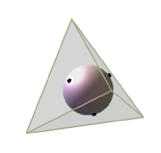
Figure 4. Tetrahedron

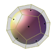
Figure 5. Regular dodecahedron

However, truncating one of the vertices as in Figure 7 does not produce a circumsolid unless the plane of truncation is chosen to match the inscribed sphere. Other examples of three-dimensional circumsolids include the platonic solids and other Archimedean solids (see for example Figure 5).

         

Figure 6. Tetrahedron with a flat top

 

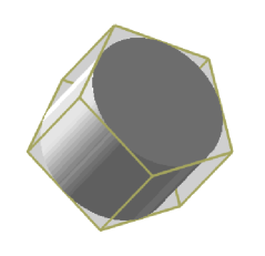
Figure 7. Prism over a regular pentagon

In the plane, the only domains which are nontrivial products of circumsolids are rectangles (products of intervals in orthogonal one-dimensional subspaces). In three dimensions, rectangular prisms (products of three intervals) are productes of circumsolids, as are prisms over planar circumsolids, such as the example in Figure 7.

               

Figure 8. Tetrahedron with non-horizontal sliced tip

We note that if $\Omega$ is a product of circumsolids then every boundary point has consistent normals, since we can define $\gamma$ by $\pi_{i}(\gamma)=-\frac{1}{R_{i}}\pi_{i}(x_{0}^{i}-x)$ for $i=1,\cdots,k$, where $x_{0}^{i}$ and $R_{i}$ are the centre and radius of the circumsolid $\Omega_{i}\subset E_{i}$ for each $i$. In the plane, every boundary point of a convex polygon has consistent normals. Figure 8 is an example of a convex polyhedron in ${\mathbb{R}}^{3}$ with vertex $x_{0}$ having inconsistent normals.

The following Theorem is the main result of this paper.

Theorem 1.2.

Let $\Omega$ be a convex polyhedral domain in ${\mathbb{R}}^{d}$, $d\geq 2$, which is not a product of circumsolids. Then for sufficiently small $\alpha>0$, the first Robin eigenfunction $u_{\alpha}$ is not log-concave.

To prove that the first Robin eigenfunction $u_{\alpha}$ admits non-convex superlevel sets in dimension $d\geq 3$, we make the following stronger assumption:

Theorem 1.3.

Let $\Omega$ be a convex polyhedral domain in ${\mathbb{R}}^{d}$. If $d=2$ and $\Omega$ is not a product of circumsolids, then the first Robin eigenfunction $u_{\alpha}$ admits non-convex superlevel sets for sufficiently small $\alpha>0$. The same conclusion holds if $d\geq 3$ and $\Omega$ has boundary points with inconsistent normals.

We stress that although Theorem 1.2 is stated for polyhedral domains, one cannot hope to avoid such non-concavity results by imposing more regularity on the boundary.

Corollary 1.4.

Let $\Omega_{0}$ be a convex polyhedral domain in ${\mathbb{R}}^{d}$, $d\geq 2$, which is not a product of circumsolids. Then for any sufficiently small $\alpha>0$, for any convex domain $\Omega$ which is sufficiently close to $\Omega_{0}$ in Hausdorff distance, the first Robin eigenfunction $u_{\alpha}$ on $\Omega$ is not log-concave.

For $\alpha<0$, the first Robin eigenvalue $\lambda_{\alpha}$ is negative, and the methods used to prove Theorem 1.2 and Corollary 1.4 also lead to the following result.

Theorem 1.5.

Let $\Omega$ be a convex polyhedral domain in ${\mathbb{R}}^{d}$, $d\geq 2$, which is not a product of circumsolids. Then for sufficiently small $\alpha<0$, the first Robin eigenfunction $u_{\alpha}$ is not log-convex. Moreover, for any convex domain $\hat{\Omega}$ which is sufficiently close to $\Omega$ in Hausdorff distance, the first Robin eigenfunction $\hat{u}_{\alpha}$ on $\hat{\Omega}$ is not log-convex.

Our approach to Theorem 1.2 is to treat the Robin problem (2.1)-(1.2) for small positive $\alpha$ as a perturbation from the Neumann case $\alpha=0$. To be more precise, let $v=\tfrac{du_{\alpha}}{d\alpha}\big{|}_{{\alpha=0}}$. Then we show in Section 3 that the function $v$ satisfies

(1.4) $$\begin{cases}\Delta v+\mu=0&\quad\text{in $\Omega$,}\\ D_{\nu}v=-1&\quad\text{on $\partial\Omega$,}\end{cases}$$

for some constant $\mu$. The concavity properties of $u_{\alpha}$ for small $\alpha$ relate directly to the concavity properties of $v$, so we proceed to investigate the latter, in the particular case of polyhedral domains. We deduce Theorem 1.2 from the statement that the solution $v$ of (1.4) on a convex polyhedral domain $\Omega$ is concave precisely when $\Omega$ is a product of circumsolids.

Our argument proceeds as follows: After some preliminary material on the perturbation problem in Section 3, we prove in Section 4 the remarkable result that every $C^{2}$ solution of (1.4) on a polyhedral domain is a quadratic function. In section 5 we relate this to concave solutions, by showing that any concave solution of (1.4) is $C^{2}$ up to the boundary. This involves expanding the solution in terms of homogeneous harmonic functions about any boundary point, and requires in particular the interesting observation that any degree two homogeneous harmonic function with bounded second derivatives and with Neumann boundary condition on a polyhedral cone in ${\mathbb{R}}^{d}$ is a quadratic function.

In Section 8 we prove that those polyhedral domains on which a quadratic function solves the equation (1.4) are products of circumsolids. This completes the preliminaries needed to prove our main Theorem 1.2 in Section 9. In the last section, we discuss some interesting observations and open problems.

2. Motivation: Log-concavity and the fundamental gap

In the case of Dirichlet boundary data, the log-concavity of the first eigenfunction is a key step in proving the lower bound of the gap between the two smallest eigenvalues [1]. In the case that the first Robin eigenfunction is log-concave, then a similar bound holds. Here we note that we can include a potential, and since we impose the strong hypothesis that the first eigenfunction is log-concave, we do not need to assume that the potential is convex.

Theorem 2.1.

Let $\lambda_{0}$ and $\lambda_{1}$ be the two smallest eigenvalues for the eigenvalue problem

(2.1) $$-\Delta u+Vu=\lambda u\text{ in $\Omega$,}$$

with Robin boundary conditions (1.2) on a bounded convex domain $\Omega$ with diameter $D$, and $V\in L^{1}_{loc}(\Omega)$. If the ground state $u_{0}$ associated to $\lambda_{0}$ is log-concave, then

(2.2) $$\lambda_{1}-\lambda_{0}\geq\frac{\pi^{2}}{D^{2}}.$$

Proof.

Let $u_{0}$ and $u_{1}$ be the eigenfunctions associated to $\lambda_{0}$ and $\lambda_{1}$ respectively. Since $u_{0}$ is positive on $\Omega$, we can set

$$v(x,t):=\frac{e^{-\lambda_{1}t}u_{1}(x)}{e^{-\lambda_{0}t}u_{0}(x)}$$

which solves the parabolic equation

(2.3) $$\dfrac{\partial v}{\partial t}=\Delta v+2D\log u_{0}\cdot Dv\quad\text{on $\Omega\times(0,+\infty)$.}$$

On the lateral boundary $\partial\Omega\times(0,+\infty)$, the normal derivative of $v$ disappears:

$$D_{\nu}v=\frac{e^{-\lambda_{1}t}}{e^{-\lambda_{0}t}}\left(\frac{D_{\nu}u_{1}}{u_{0}}-\frac{u_{1}D_{\nu}u_{0}}{u_{0}^{2}}\right)=v\left(-\alpha+\alpha\right)=0.$$

By hypothesis, $u_{0}$ is log-concave, so the drift term in (2.3) given by $X:=2\,D\log u_{0}$ satisfies the modulus of contraction inequality

$$\Big{(}X(y,t)-X(x,t)\Big{)}\cdot\frac{y-x}{\lvert y-x\rvert}\leq 0$$

corresponding to the modulus of contraction $\omega\equiv 0$. Therefore by [1, Theorem 2.1], for some large constant $C>0$, the function

$$\varphi(s,t):=Ce^{-\frac{\pi^{2}}{D^{2}}t}\sin\left(\frac{\pi s}{D}\right)\quad\text{for every $s\in[0,D/2]$, $t\geq 0$,}$$

is a modulus of continuity for $v$, that is,

$$v(y,t)-v(x,t)\leq 2\,\varphi\left(\tfrac{y-x}{\lvert y-x\rvert},t\right)\quad\text{for every $x$, $y\in\overline{\Omega}$, $t\geq 0$,}$$

where $\frac{\pi^{2}}{D^{2}}$ is the second (or the difference of the second and first) Neumann eigenvalue on the interval. From this, we can deduce that

$$e^{-(\lambda_{1}-\lambda_{0})t}\operatorname*{osc}_{\overline{\Omega}}\left(\frac{u_{1}}{u_{0}}\right)\leq C\,e^{-\frac{\pi^{2}}{D^{2}}t}\quad\text{for all $t\geq 0$,}$$

which can only hold if inequality (2.2) holds. This completes the proof of Theorem 2.1. ∎

The argument given follows the approach used in the Dirichlet case [1]. A similar result would follow using the gradient estimate approach of [19, 23].

The resulting estimate is sharp in the case $\alpha=0$, where it is the Payne-Weinberger inequality for the first nontrivial Neumann eigenvalue [18, 24]. Otherwise, it is not sharp, as can be seen from the one dimensional case, where the eigenvalues can be computed. It is appealing to conjecture that the sharp lower bound for given $\alpha$ and $D$ should correspond to the gap for the corresponding one-dimensional problem, which would result in an estimate which depends on $\alpha$ and increases from $\frac{\pi^{2}}{D^{2}}$ to $\frac{3\pi^{2}}{D^{2}}$ as $\alpha$ increases from $0$ towards infinity. However, our main theorem (Theorem 1.2, that the ground state is in general not log-concave) means that a sharp result must necessarily be proved by rather different means.

3. The Robin eigenvalue problem and perturbations

We recall some properties of the first Robin eigenvalue $\lambda_{\alpha}$ and the corresponding eigenfunction $u_{\alpha}$. These results are quite well established [13], see also [14, Theorem 1.3.1] or [11], however we include a proof for the convenience of the reader.

Proposition 3.1.

Let $\Omega$ be a connected bounded Lipschitz domain in ${\mathbb{R}}^{d}$. Then

1. For every $\alpha\in{\mathbb{R}}$, there is a first Robin eigenvalue $\lambda_{\alpha}\in{\mathbb{R}}$ with a positive eigenfunction $u_{\alpha}\in H^{1}(\Omega)$.

2. For every $\alpha\in{\mathbb{R}}$, the first Robin eigenvalue $\lambda_{\alpha}$ is simple.

3. The function $\alpha\mapsto\lambda_{\alpha}$ is differentiable, with derivative given by

   (3.1) $$\dot{\lambda}_{\alpha}=\frac{\int_{\partial\Omega}u_{\alpha}^{2}\,\mathrm{d}\mathcal{H}}{\int_{\Omega}u_{\alpha}^{2}\,\mathrm{d}x}\geq 0.$$

4. The positive Robin eigenfunction $u_{\alpha}$ (normalised to have $\tfrac{1}{\lvert\Omega\rvert}\int_{\Omega}u_{\alpha}^{2}\ \,\mathrm{d}x=1$) is $C^{1}$-dependent on $\alpha$ in $H^{1}(\Omega)$ and in $C^{0,\beta}(\Omega)$ for some $\beta\in(0,1)$. More precisely, $u_{\alpha}$ is continuously dependent on $\alpha$ in $H^{1}(\Omega)$ and in $C^{0,\beta}(\Omega)$, and if for $\alpha_{0}\in{\mathbb{R}}$, $v$ is the unique solution, orthogonal to $u_{\alpha_{0}}$ in $L^{2}(\Omega)$, of

   (3.2) $$\begin{cases}\Delta v+\lambda_{\alpha_{0}}v=-\dot{\lambda}_{\alpha_{0}}u_{\alpha_{0}}&\text{in $\Omega$,}\\ \;D_{\nu}v+\alpha_{0}v=-u_{\alpha_{0}}&\text{on $\partial\Omega$,}\\ \end{cases}$$

   then $u_{\alpha}=u_{\alpha_{0}}+v\,(\alpha-\alpha_{0})+o(\alpha-\alpha_{0})$ for every $\alpha$ in a neighbourhood of $\alpha_{0}$, where $o(\alpha-\alpha_{0})/(\alpha-\alpha_{0})\to 0$ in $H^{1}(\Omega)\cap C^{0,\beta}(\Omega)$ as $\alpha\to\alpha_{0}$.

Proof.

We begin by showing that for every $\alpha\in{\mathbb{R}}$, there is a first Robin eigenvalue $\lambda_{\alpha}\in{\mathbb{R}}$. For every $M>0$, let $[\cdot,\cdot]_{M}$ be given by

$$[u,v]_{M}:=\int_{\Omega}Du\,Dv\,\mathrm{d}x+M\int_{\Omega}u\,v\,\mathrm{d}x$$

for every $u$, $v\in H^{1}(\Omega)$. Then $[\cdot,\cdot]_{M}$ is an inner product on $H^{1}(\Omega)$, which by the theorem of the bounded inverse [5, Corollary 2.7] is equivalent to the usual inner product on $H^{1}(\Omega)$. We denote by $\lVert\cdot\rVert_{M}$ the norm on $H^{1}(\Omega)$ induced by $[\cdot,\cdot]_{M}$. For the rest of this proof, we denote by $H^{1}_{M}(\Omega)$ the Hilbert space $H^{1}(\Omega)$ equipped with the inner product $[\cdot,\cdot]_{M}$, and set

$$\tau(u,v)=\int_{\partial\Omega}u\,v\,\mathrm{d}\mathcal{H}\quad\text{and}\\ quadquadb(u,v)=\int_{\Omega}u\,v\,\mathrm{d}\mathcal{H}$$

for every $u$, $v\in H^{1}_{M}(\Omega)$. The bilinear forms $\tau$ and $b$ on $H^{1}_{M}(\Omega)$ are bounded. Hence, by the Riesz-Fréchet representation theorem [5, Theorem 5.5], for every $u\in H^{1}_{M}(\Omega)$, there are unique $Tu\in H^{1}_{M}(\Omega)$ and $Bu\in H^{1}_{M}(\Omega)$ satisfying

(3.3) $$[Tu,v]_{M}=\tau(u,v)\quad\text{and}\quad[Bu,v]_{M}=b(u,v)$$

$v\in H^{1}_{M}(\Omega)$. This defines bounded linear mappings $T$ and $B$ on $H^{1}_{M}(\Omega)$. Since $H^{1}(\Omega)$ is compactly embedded in $L^{2}(\Omega)$, $B$ is also a compact linear operator on $H^{1}_{M}(\Omega)$. We employ the two operators $\alpha T$ and $B$ to characterise Robin eigenfunctions. First, recall that for every $\alpha\in{\mathbb{R}}$, $u\in H^{1}(\Omega)\setminus\{0\}$ is a Robin eigenfunction to eigenvalue $\lambda_{\alpha}$ if and only if $u$ satisfies

$$\int_{\Omega}Du\,Dv\,\mathrm{d}x+\alpha\int_{\partial\Omega}u\,v\,\mathrm{d}\mathcal{H}=\lambda_{\alpha}\,\int_{\Omega}u\,v\,\mathrm{d}x$$

for every $v\in H^{1}(\Omega)$, or equivalently for every $M>0$,

$$\int_{\Omega}Du\,Dv\,\mathrm{d}x+M\int_{\Omega}u\,v\,\mathrm{d}x+\int_{\partial\Omega}u\,v\,\mathrm{d}\mathcal{H}=(\lambda_{\alpha}+M)\,\int_{\Omega}u\,v\,\mathrm{d}x$$

for every $v\in H^{1}(\Omega)$. Thus, if $I$ is the identity operator then the above is equivalent to

$$(I+\alpha T)u=(\lambda_{\alpha}+M)Bu\quad\text{in $H^{1}(\Omega)$.}$$

By the continuity of the trace operator on $W^{1,1}(\Omega)$ (cf [16, Theorem 15.8]) and Young’s inequality, we find that for all $\varepsilon>0$, there is $C_{\varepsilon}>0$ such that

$$\lVert v\rVert_{L^{2}(\partial\Omega)}^{2}\leq\varepsilon\,\lVert Dv\rVert_{L^{2}(\Omega)}^{2}+C_{\varepsilon}\lVert v\rVert_{L^{2}(\Omega)}^{2}$$

for every $v\in H^{1}(\Omega)$ and so by choosing $M_{\varepsilon}=C_{\varepsilon}/\varepsilon$, we obtain that

(3.4) $$\lVert v\rVert_{L^{2}(\partial\Omega)}\leq\sqrt{\varepsilon}\,\left(\lVert Dv\rVert_{L^{2}(\Omega)}^{2}+\tfrac{C_{\varepsilon}}{\varepsilon}\lVert v\rVert_{L^{2}(\Omega)}^{2}\right)^{1/2}=\sqrt{\varepsilon}\,\lVert v\rVert_{M_{\varepsilon}}$$

for every $v\in H^{1}(\Omega)$. Applying Cauchy-Schwarz’s inequality and (3.4), we see

$$\lVert Tu\rVert_{M_{\varepsilon}}^{2}=[Tu,Tu]_{M_{\varepsilon}}=\tau(u,u)\leq\lVert u\rVert_{L^{2}(\partial\Omega)}\,\lVert Tu\rVert_{L^{2}(\partial\Omega)}\leq\varepsilon\,\lVert u\rVert_{M_{\varepsilon}}\,\lVert Tu\rVert_{M_{\varepsilon}},$$

proving that for every $\varepsilon>0$, the operator $T$ on $H^{1}(\Omega),[\cdot,\cdot]_{M_{\varepsilon}}$ has operator norm $\lVert T\rVert_{\mathcal{L}(H^{1}(\Omega))}\leq\varepsilon$. Now, for given $\alpha\in{\mathbb{R}}$, we fix $\varepsilon>0$ such that $\lvert\alpha\rvert<\tfrac{1}{\varepsilon}$. It follows that the operator $\alpha T$ on $(H^{1}(\Omega),[\cdot,\cdot]_{M_{\varepsilon}})$ has operator norm $\lVert-\alpha T\rVert_{\mathcal{L}(H^{1}(\Omega))}<1$. Hence the operator $I+\alpha T$ is invertible on $H^{1}(\Omega)$, and so $u_{\alpha}\in H^{1}(\Omega)$ is a Robin eigenfunction with eigenvalue $\lambda_{\alpha}$ if and only if $u_{\alpha}$ is an eigenfunction of the operator $T_{\alpha}:=(I+\alpha T)^{-1}B$ for the eigenvalue $\lambda_{\alpha}+M_{\varepsilon}$. Note, for every $\alpha\in{\mathbb{R}}$, $T_{\alpha}$ is compact on $H^{1}(\Omega)$ since $(I+\alpha T)^{-1}$ is bounded and $B$ is compact on $H^{1}(\Omega)$. Therefore [5, Theorems 6.6 & 6.8], for every $\alpha\in{\mathbb{R}}$, the point spectrum $\sigma_{p}(T_{\alpha})$ of $T_{\alpha}$ consists of a sequence $(\Lambda_{\alpha}^{(j)})_{j\geq 1}$ of eigenvalues $\Lambda_{\alpha}^{(j)}\in{\mathbb{R}}\setminus\{0\}$ of finite algebraic and geometric mulitiplicity. In particular, this proves the existence of the first Robin eigenvalue $\lambda_{\alpha}:=\tfrac{1}{\Lambda_{\alpha}(1)}-M_{\varepsilon}\in{\mathbb{R}}$ for every $\alpha\in{\mathbb{R}}$ (for $\alpha=0$, $\lambda_{\alpha}=0$ is the first Neumann eigenvalue). The eigenspace of $\lambda_{\alpha}$ is one-dimensional (see [14, Theorem 1.3.1]) and admits a positive eigenfunction $u_{\alpha}\in H^{1}(\Omega)$ satisfying the normalisation $\int_{\Omega}u_{\alpha}^{2}\,\mathrm{d}x=1$. Now, the family $(T_{\alpha})_{\alpha\in{\mathbb{R}}}$ of compact operators $T_{\alpha}$ satisfies the hypotheses of [13, Theorem 2.6 of Chapter 8.2]. Thus, statement (4) with respect to the topology given by $H^{1}(\Omega)$ holds. Furthermore, if we apply [17, Theorem 3.14] to the function $w:=u_{\hat{\alpha}}-u_{\alpha}-v(\hat{\alpha}-\alpha)$, then we see that statement (4) holds with respect to the topology given by $C^{0,\beta}(\Omega)$ for some $\beta\in(0,1)$. ∎

Next, we state a convergence result on Robin problems on varying domains, which is a slight improvement of [6, Corollary 3.4]. For this, we recall the definition of the Hausdorff complementary topology on open sets (cf [6, Section 2]). For closed subsets $F_{1}$, $F_{2}$ in ${\mathbb{R}}^{d}$, the Hausdorff metric $d_{\mathcal{H}}$ is defined by

$$d_{\mathcal{H}}(F_{1},F_{2})=\max\Big{\{}\sup_{x\in F_{1}}\textrm{dist}(x,F_{2}),\sup_{x\in F_{2}}\inf_{y\in F_{1}}\lvert x-y\rvert\Big{\}},$$

where $\textrm{dist}(x,F_{i}):=\inf_{y\in F_{i}}\lvert x-y\rvert$ with the standard conventions $\textrm{dist}(x,\emptyset)=+\infty$ so that $d_{\mathcal{H}}(x,F)=0$ if $F=\emptyset$ and $d_{H}(\emptyset,F):=+\infty$ if $F\not=\emptyset$. Let $\Omega^{c}={\mathbb{R}}^{d}\setminus\Omega$ be the complement of $\Omega$. Now, a sequence $(\Omega_{n})_{n\geq 1}$ of open sets $\Omega_{n}$ in ${\mathbb{R}}^{d}$ converges to the open set $\Omega$ in ${\mathbb{R}}^{d}$ in the Hausdorff complementary topology, which we write as $\Omega_{n}\to\Omega$ in $\mathcal{H}^{c}$, if for every closed ball $B$ in ${\mathbb{R}}^{d}$, one has that $d_{H}(B\cap\Omega_{n}^{c},B\cap\Omega^{c})\to 0$ as $n\to\infty$.

Proposition 3.2.

For $d\geq 1$, let $D\subseteq{\mathbb{R}}^{d}$ be an open and bounded set, and let $\Omega$ and $\Omega_{n}$ be open domains with a Lipschitz continuous boundary satisfying $\Omega$, $\Omega_{n}\subset\subset D$. Let

$$\Omega_{n}\to\Omega\text{ in $\mathcal{H}^{c}$,}\quad\lvert\Omega_{n}\rvert\to\lvert\Omega\rvert,\quad\mathcal{H}^{d-1}(\partial\Omega_{n})\to\mathcal{H}^{d-1}(\partial\Omega)$$

as $n\to+\infty$. Furthermore, for $\alpha>0$, let $\lambda_{\alpha,n}$ and $\lambda_{\alpha}$ be the first Robin eigenvalue on $\Omega_{n}$ and $\Omega$, and let $u_{\alpha,n}$ and $u_{\alpha}$ be the first positive Robin eigenfunctions with unit $L^{2}(\Omega)$-norm. Then

(3.5) $$\lambda_{\alpha,n}\to\lambda_{\alpha}\quad\text{as $n\to+\infty$,}$$

(3.6) $$u_{\alpha,n}\,\mathds{1}_{\Omega_{n}}\to u_{\alpha}\,\mathds{1}_{\Omega}\quad\text{in $H^{1}(D)$ as $n\to+\infty$.}$$

Furthermore, there are $\gamma\in(0,1)$ and $C>0$ such that

(3.7) $$\lVert u_{\alpha,n}\rVert_{C^{0,\gamma}(\overline{\Omega}_{n})}\leq C\quad\text{for all $n\geq 1$,}$$

and for every non-empty set $B\subseteq\bigcap_{n\geq n_{0}}\overline{\Omega}_{n}$, $n_{0}\geq 1$, and $0\leq\hat{\gamma}<\gamma$, there is a subsequence $(u_{\alpha,\hat{n}})_{\hat{n}\geq 1}$ of $(u_{\alpha,\hat{n}})_{\hat{n}\geq 1}$ such that

(3.8) $$u_{\alpha,\hat{n}}\to u_{\alpha}\quad\text{in $C^{0,\hat{\gamma}}(B)$ as $\hat{n}\to+\infty$.}$$

Proof.

Under the hypotheses of this Proposition, [6, Corollary 3.4] implies (3.1). Thus,

(3.9) $$\begin{split}\lim_{n\to+\infty}\lVert Du_{\alpha,n}\rVert_{L^{2}(\Omega_{n};{\mathbb{R}}^{d})}^{2}+\alpha\lVert u_{\alpha,n}\rVert_{L^{2}(\partial\Omega_{n})}^{2}&=\lim_{n\to+\infty}\lambda_{\alpha,n}\\ &=\lambda_{\alpha}\\ &=\lVert Du_{\alpha}\rVert_{L^{2}(\Omega;{\mathbb{R}}^{d})}^{2}+\alpha\lVert u_{\alpha}\rVert_{L^{2}(\partial\Omega)}^{2}.\end{split}$$

Since $\Omega_{n}\subseteq D$ for all $n\geq 1$, we can conclude from the limit (3.9) and by [6, Lemma 4.2 and Lemma 4.7] that limit (3.6) holds strongly in $L^{2}(D)$ and weakly in $H^{1}(D)$. Moreover, by limit (3.9) and since $Du_{\alpha,n}\,\mathds{1}_{\Omega_{n}}\to Du_{\alpha}\,\mathds{1}_{\Omega}$ weakly in $L^{2}(D;R^{d})$ as $n\to+\infty$ and by [6, Lemma 4.7], it follows that limit (3.6) holds in $H^{1}(D)$. Finally, bound (3.7) and limit (3.8) in $C^{0,\hat{\gamma}}(B)$ for every non-empty set $B\subseteq\bigcap_{n\geq 1}\overline{\Omega}_{n}$ and $0\leq\hat{\gamma}<\gamma$ are consequences from [17, Proposition 3.6]. ∎

4. Regular solutions are quadratic

When $\alpha=0$, the perturbation problem (3.2) reduces to equation (1.4), with the constant $\mu$ computed by integrating the first equation over $\Omega$ and applying the boundary condition, yielding $\mu={\mathcal{H}}^{d-1}(\partial\Omega)/\mathcal{H}^{d}(\Omega)$.

In this and the next several sections we consider a class of problems generalising (1.4), under the assumption that $\Omega$ is a convex polyhedral domain in ${\mathbb{R}}^{d}$ for $d\geq 2$. More precisely, this means that $\Omega$ is the intersection of finitely many open half-spaces:

$$\Omega=\bigcap_{i=1}^{m}\Big{\{}x\in{\mathbb{R}}^{d}\,\Big{|}\,x\cdot\nu_{i}<b_{i}\Big{\}},$$

and we can assume without loss of generality that the description is minimal, meaning that omitting any one of the half-spaces from the intersection results in a strictly larger set. In this case $\Omega$ has $m$ faces

$$\Sigma_{i}=\Big{\{}x\in\overline{\Omega}\,\Big{|}\ \nu_{i}\cdot x=b_{i}\Big{\}}$$

for $i=1,\dots,m$, each of which is itself a convex polyhedral subset of the affine subspace $\{x\in{\mathbb{R}}^{d}\,|\ \nu_{i}\cdot x=b_{i}\}$. The outer unit normal to $\Omega$ on the face $\Sigma_{i}$ is $\nu_{i}$.

For an open convex set $\Omega$ in ${\mathbb{R}}^{d}$, the tangent cone $\Gamma_{x}$ to $\Omega$ at a point $x\in\overline{\Omega}$ is defined by

$$\Gamma_{x}=\Big{\{}r(y-x)\;\Big{|}\;y\in\Omega,\ r>0\Big{\}}=\bigcup_{r>0}r(\Omega-x).$$

If $x$ is in $\Omega$, the tangent cone $\Gamma_{x}$ is simply $\mathbb{R}^{d}$. In the case of polyhedral domains, the tangent cone can be described as follows: For each point $x\in\overline{\Omega}$, let

(4.1) $$\mathcal{I}(x):=\Big{\{}i\in\{1,\dots,m\}\;\Big{|}\;x\cdot\nu_{i}=b_{i}\Big{\}}$$

index the faces touching $x$, then the tagent cone

$$\Gamma_{x}=\bigcap_{i\in{\mathcal{I}}(x)}\Big{\{}y\;\Big{|}\;y\cdot\nu_{i}<0\Big{\}}.$$

This is a cone over the subset $A_{x}=\Gamma_{x}\cap{\mathbb{S}}^{d-1}$ of the unit sphere. In particular, $\Gamma_{x}$ is the intersection of finitely many half-spaces with the origin in their common boundary. We call such a set a polyhedral cone.

Remark 4.1.

A special feature of polyhedral domains is that for every $x\in\overline{\Omega}$ there exists $r>0$ such that $B_{r}(x)\cap\Omega=x+\left(B_{r}(0)\cap\Gamma_{x}\right)$, so that $\Omega$ is a cone near $x$.

We now establish a version of the strong maximum principle on general open cones $\Gamma$ with a Lipschitz boundary. In this paper, our application of Proposition 4.2 remains on cones with a polyhedral structure.

Proposition 4.2.

Let $\Gamma$ be an open cone with Lipschitz boundary and vertex at the origin in ${\mathbb{R}}^{d}$, and $r>0$. Let $w\in H^{1}(B_{r}(0)\cap\Gamma)$ be a weak solution of

(4.2) $$\begin{cases}\Delta w=0&\text{on}\ B_{r}(0)\cap\Gamma,\\ D_{\nu}w=0&\text{on}\ B_{r}(0)\cap\partial\Gamma.\end{cases}$$

If $w(0)=0$ and $w\leq 0$ on $B_{r}(0)\cap\Gamma$, then $w\equiv 0$ on $B_{r}(0)\cap\Gamma$.

By scaling it suffices to consider the case $r=1$. We begin by setting $A=S^{d-1}\cap\Gamma$. Then the set $B_{1}(0)\cap\Gamma$ can be described by the polar coordinate map

$$(r,z)\in(0,1)\times A\mapsto rz\in B_{1}(0)\cap\Gamma.$$

Since the set $A$ is a Lipschitz domain in ${\mathbb{S}}^{d-1}$, there is a complete $L^{2}(A)$-orthonormal set of eigenfunctions $\{\varphi_{i}\}_{i=0}^{\infty}$ for the Neumann Laplacian on $A$, with associated eigenvalues $\lambda_{i}$ which we arrange in non-decreasing order with $\lambda_{0}=0$. Let $w\in H^{1}(B_{1}(0)\cap\Gamma)$. Then for every $r\in(0,1)$, $w\in H^{1}(\ B_{r}(0)\cap\Gamma)$, the trace $w(r,\cdot)$ of $w$ exists in $L^{2}(A)$. Using this, we see that $w$ can be rewritten in polar coordinates as

(4.3) $$w(r,z)=\sum_{i=0}^{\infty}w_{i}(r)\varphi_{i}(z)\quad\text{for every $(r,z)\in[0,1)\times A$,}$$

where for every $r\in(0,1)$ and $i\geq 1$,

(4.4) $$w_{i}(r):=(w(r,\cdot),\varphi_{i})_{L^{2}(A)}$$

is the $i$th Fourier coefficient of the trace of $w(r,\cdot)$ in $L^{2}(A)$. In order to continuous the proof of Proposition 4.2, we need to establish first some more properties of the series decomposition (4.3) of the weak solution $w$ of (4.2). This is done in the next two statements.

Lemma 4.3.

Let $\Gamma$ be an open cone with Lipschitz boundary and vertex at the origin in ${\mathbb{R}}^{d}$, and let $w\in H^{1}(B_{1}(0)\cap\Gamma)$ be a weak solution of Neumann problem (4.2). Then for all $i\geq 1$,

(4.5) $$f_{i}:=\lim_{r\to 1}w_{i}(r)$$

exists, and furthermore the series $\sum_{i=0}^{\infty}\sqrt{1+\lambda_{i}}f_{i}^{2}$ converges with

(4.6) $$\sum_{i=0}^{\infty}\sqrt{1+\lambda_{i}}f_{i}^{2}\leq C\,\lVert w\rVert_{H^{1}(B_{1}(0)\cap\Gamma)}^{2}.$$

Proof.

The $H^{1}(B_{1}(0)\cap\Gamma)$-norm of $w$ can be written as

(4.7) $$\begin{split}\lVert w\rVert_{H^{1}(B_{1}(0)\cap\Gamma)}^{2}&=\int_{B_{1}(0)\cap\Gamma}w^{2}+|Dw|^{2}\,d{\mathcal{H}}^{d}\\ &=\sum_{i,j=0}^{\infty}\left\{\int_{0}^{1}\left(w_{i}w_{j}+w_{i}^{\prime}w_{j}^{\prime}\right)r^{d-1}\,dr\int_{A}\varphi_{i}\varphi_{j}d{\mathcal{H}}^{d-1}(z)\right\}\\ &\qquad\hbox{}+\sum_{i,j=1}^{\infty}\left\{\int_{0}^{1}w_{i}w_{j}r^{d-3}dr\int_{A}D\varphi_{i}\cdot D\varphi_{j}\,d{\mathcal{H}}^{d-1}(z)\right\}\\ &=\sum_{i=0}^{\infty}\int_{0}^{1}\left(\Big{(}1+\frac{\lambda_{i}}{r^{2}}\Big{)}\,w_{i}^{2}+(w_{i}^{\prime})^{2}\right)r^{d-1}\,dr,\end{split}$$

where $w_{i}^{\prime}(r)=\frac{dw_{i}}{dr}(r)=\int_{A}\nabla w(r,z)\cdot z\,\varphi_{i}(z)\,d\mathcal{H}^{d-1}(z)$ and

$$\int_{A}D\varphi_{i}\cdot D\varphi_{j}\,d{\mathcal{H}}^{d-1}=-\int_{A}\Delta\varphi_{i}\varphi_{j}\,d{\mathcal{H}}^{d-1}=\lambda_{i}\int_{A}\varphi_{i}\varphi_{j}\,d{\mathcal{H}}^{d-1}=\lambda_{i}\delta_{ij}.$$

Let $\delta\in(0,1)$ and consider the mapping $g:[\delta,1)\to L^{2}(A)$ defined by

$$g(r)=\sum_{i=0}^{\infty}\sqrt{1+\lambda_{i}}\,w_{i}^{2}(r)\quad\text{for every $r\in[\delta,1)$.}$$

Then

$$\left\lvert\frac{d}{dr}g(r)\right\rvert=\left\lvert 2\sum_{i=0}^{\infty}\sqrt{1+\lambda_{i}}\,w_{i}w_{i}^{\prime}\right\rvert\leq\sum_{i=0}^{\infty}w_{i}^{2}\Big{(}1+\frac{\lambda_{i}}{r^{2}}\Big{)}+\sum_{i=0}^{\infty}\left(w_{i}^{\prime}\right)^{2}$$

and so

(4.8) $$\begin{split}\lvert g(r_{2})-g(r_{1})\rvert&\leq\int_{r_{1}}^{r_{2}}\left\lvert\frac{d}{dr}g(r)\right\rvert\,\mathrm{d}r\\ &\leq\int_{r_{1}}^{r_{2}}\sum_{i=0}^{\infty}(1+\frac{\lambda_{i}}{r^{2}})w_{i}^{2}+\sum_{i=0}^{\infty}\left(w_{i}^{\prime}\right)^{2}\,dr\\ &\leq C_{\delta}\sum_{i=0}^{\infty}\int_{r_{1}}^{r_{2}}\left((1+\frac{\lambda_{i}}{r^{2}})w_{i}^{2}+(w_{i}^{\prime})^{2}\right)r^{d-1}\,dr.\end{split}$$

for every $0<\delta<r_{1}<r_{2}<1$. By (4.7), the right hand side in the last estimate of (4.8) tends to zero as $r_{1}$, $r_{2}\to 1^{-}$. Hence, the Cauchy criterion implies that

$$\lim_{r\to 1^{-}}g(r)=\sum_{i=0}^{\infty}\sqrt{1+\lambda_{i}}\,f_{i}^{2}\quad\text{exists,}$$

where $f_{i}$ is defined by (4.5). This shows that the function $g$ is absolutely continuous on $[\delta,1]$ for every $\delta\in(0,1)$. By the mean value theorem for integrals, there is an $r_{\delta}\in(\delta,1)$ satisfying

$$g(r_{\delta})=\tfrac{1}{1-\delta}\int_{\delta}^{1}g(r)dr=\tfrac{1}{1-\delta}\sum_{i=0}^{\infty}\int_{\delta}^{1}\sqrt{1+\lambda_{i}}w_{i}^{2}\,dr\leq\tfrac{C_{\delta}}{1-\delta}\lVert w\rVert_{H^{1}(B_{1}(0)\cap\Gamma)}^{2},$$

where we also used (4.8) and (4.7). Using this together with (4.8), one finds

$$g(r)=g(r)-g(r_{\delta})+g(r_{\delta})\leq C\,\lVert w\rVert_{H^{1}(B_{1}(0)\cap\Gamma)}^{2}$$

for some $C>0$ independent of $r\in(\delta,1)$. Sending $r\to 1$, we find (4.6). ∎

Due to Lemma 4.3, every weak solution $w$ of (4.2) has the following series expansion.

Proposition 4.4.

Let $\Gamma$ be an open cone with Lipschitz boundary and vertex at the origin in ${\mathbb{R}}^{d}$, and follow the notation of Lemma 4.3. Then every weak solution $w\in H^{1}(B_{1}(0)\cap\Gamma)$ of (4.2) satisfies

(4.9) $$w(rz)=\sum_{i=0}^{\infty}f_{i}\,r^{\beta_{i}}\varphi_{i}(z)\quad\text{for every $z\in A$ and $r\in(0,1)$.}$$

The convergence of the series holds in $H^{1}(B_{1}(0)\cap\Gamma)\cap C^{\gamma_{r}}(\overline{B_{r}(0)\cap\Gamma})$ for every $0<r<1$, where $\gamma_{r}\in(0,1)$, and for every integer $i\geq 0$, $\beta_{i}\geq 0$ solves

(4.10) $$\beta_{i}^{2}+(d-2)\beta_{i}-\lambda_{i}=0.$$

We will often use (4.10) in the form $\beta_{i}=\frac{1}{2}\left(d-2+\sqrt{(d-2)^{2}+4\lambda_{i}}\right)$.

Proof.

We define

$$\psi_{i}(rz):=r^{\beta_{i}}\varphi_{i}(z)\quad\text{for every $rz\in B_{1}(0)\cap\Gamma$.}$$

Then $\psi_{i}$ is harmonic on $B_{1}(0)\cap\Gamma$ since

$$\Delta(r^{\beta}_{i}\varphi_{i}(z)) =r^{\beta_{i}-2}\Delta_{{\mathbb{S}}^{d-1}}\varphi_{i}+(d-1)\frac{\partial r^{\beta_{i}}}{\partial r}\varphi_{i}+\frac{\partial^{2}r^{\beta_{i}}}{\partial r^{2}}\varphi_{i}$$

$$=r^{\beta_{i}-2}\left(-\lambda_{i}+({d-2})\beta_{i}+\beta_{i}^{2}\right)\varphi_{i}$$

$$=0$$

by (4.10) and the fact that $\varphi_{i}$ satisfies

(4.11) $$\Delta^{{\mathbb{S}}^{d-1}}\varphi_{i}+\lambda_{i}\varphi_{i}=0\quad\text{ on $A$.}$$

Furthermore, $\psi_{i}$ satisfies Neumann boundary conditions on $B_{1}(0)\cap\partial\Gamma$, since $\varphi_{i}$ satisfies Neumann conditions on $\partial A$. Thus, each $\psi_{i}$ is a weak solution of (4.2).

Now, let $\tilde{w}:B_{1}(0)\cap\partial\Gamma\to{\mathbb{R}}$ be given by

$$\tilde{w}(r,z):=\sum_{i=0}^{\infty}f_{i}\,\psi_{i}(rz)=\sum_{i=0}^{\infty}f_{i}\,r^{\beta_{i}}\,\varphi_{i}(z)\quad\text{for every $rz\in B_{1}(0)\cap\Gamma$,}$$

where $f_{i}$ is given by (4.5). Next, we show that the infinite series of $\tilde{w}$ converges in $H^{1}(B^{1}(0)\cap\Gamma)$. For this, let $\tilde{w}^{N}$ be the partial sum of $\tilde{w}$ given by

$$\tilde{w}^{N}(r,z)=\sum_{i=0}^{N}f_{i}\,r^{\beta_{i}}\varphi_{i}(z)\quad\text{for every $rz\in B_{1}(0)\cap\Gamma$.}$$

For integers $1\leq M<N$, applying (4.7) to $\tilde{w}^{N}-\tilde{w}^{M}=\sum_{i=M+1}^{N}f_{i}r^{\beta_{i}}\varphi_{i}$, we find

$$\lVert\tilde{w}^{N}-\tilde{w}^{M}\rVert_{H^{1}(B_{1}(0)\cap\Gamma)}^{2} =\sum_{i=M+1}^{N}\int_{0}^{1}\left(f_{i}^{2}r^{2\beta_{i}+d-1}+\beta_{i}^{2}f_{i}^{2}r^{2\beta_{i}+d-3}\right)\,dr$$

$$=\sum_{i=M+1}^{N}\left(\frac{1}{2\beta_{i}+d}+\frac{\beta_{i}^{2}}{2\beta_{i}+d-2}\right)f_{i}^{2}$$

$$\leq C\sum_{i=M+1}^{N}\left(\beta_{i}+1\right)f_{i}^{2}$$

$$\leq C\sum_{i=M+1}^{N}\sqrt{1+\lambda_{i}}f_{i}^{2}.$$

Lemma 4.3 implies that the infinite series $\sum_{i=0}^{\infty}\sqrt{1+\lambda_{i}}f_{i}^{2}$ is convergent, and so there is $\tilde{w}\in H^{1}(B_{1}(0)\cap\Gamma)$ such that $\tilde{w}^{N}$ converges to $\tilde{w}$ in $H^{1}(B_{1}(0)\cap\Gamma)$. Since every partial sum $\tilde{w}^{N}$ is a weak solution of (4.2), the limit function $\tilde{w}$ is also a weak solution of (4.2) and has $L^{2}$-trace

$$\sum_{i=0}^{\infty}f_{i}\,\varphi_{i}\quad\text{on $A$.}$$

Since the same is true for $w$, we have $w=\tilde{w}$, proving that (4.9) holds in $H^{1}(B_{1}(0)\cap\Gamma)$. To obtain convergence of the series (4.3) in $C^{\gamma_{r}}(\overline{B_{r}(0)\cap\Gamma})$ for every $0<r<1$ with some $\gamma_{r}\in(0,1)$, we employ a reflection argument in a small neighbourhood $U$ of each boundary point of $B_{r}(0)\cap\partial\Gamma$ as in [17] and use the interior Hölder-regularity result [12, Theorem 8.24]. Further, we can cover $\overline{B_{r}(0)\cap\Gamma}\setminus\partial\Gamma$ by finitely many balls and apply again the interior Hölder-regularity to $w$. Summarising, we see that for every $0<r<1$, there is a $\gamma_{r}\in(0,1)$ such that the series (4.3) converges in $C^{\gamma}_{r}(\overline{B_{r}(0)\cap\Gamma})$. ∎

With the above preliminary results established, we can prove Proposition 4.2:

Proof of Proposition 4.2.

Since $w(0)=0$ and $\beta_{i}>0$ for $i>0$, we have $f_{0}=0$. Note that $\beta_{i}$ is non-decreasing in $\lambda_{i}$ and hence in $i$.

Now assume $w$ is not identically zero. Let $f_{i_{0}}$ be the first non-zero coefficient, so that we have

$$w(r,z)=r^{\beta_{i_{0}}}\left(\sum_{{\beta_{i}=\beta_{i_{0}}}}f_{i}\varphi_{i}(z)+\sum_{\beta_{i}>\beta_{i_{0}}}f_{i}r^{\beta_{i}-\beta_{i_{0}}}\varphi_{i}(z)\right).$$

The bracket on the right is non-positive since $w\leq 0$, and the second term converges uniformly to zero in $z$ as $r$ approaches zero, while the first term is constant in $r$. Hence we have that the term

$$h(z):=\sum_{\beta=\beta_{i_{0}}}f_{i}\varphi_{i}(z)\leq 0\quad\text{for all $z\in A$.}$$

But $h$ is a non-constant Neumann eigenfunction on the connected domain $A$, and hence changes sign. This is a contradiction, and so $w$ must be identically zero as claimed in Proposition 4.2. ∎

Although we are mostly interested in the perturbation problem (1.4), the results of this section and the next also apply for a somewhat larger class: We consider (weak) solutions $v$ of the problem

(4.12) $$\begin{cases}\Delta v+\mu=0&\quad\text{in\ }\Omega,\\ D_{\nu_{i}}v+\gamma_{i}=0&\quad\text{on\ }\Sigma_{i}.\end{cases}$$

where $\mu$ and $\gamma_{1},\cdots,\gamma_{m}$ are constants. We observe (by integration of the first equation over $\Omega$ and application of the boundary condition on each face $\Sigma_{i}$) that these constants necessarily satisfy the relation

$$\sum_{i=1}^{m}\gamma_{i}{\mathcal{H}}^{d-1}(\Sigma_{i})=\mu\mathcal{H}^{d}(\Omega).$$

The main result of this section is the following:

Theorem 4.5.

Let $\Omega$ be a polyhedral domain in ${\mathbb{R}}^{d}$ with faces $\Sigma_{1},\dots,\Sigma_{m}$ and $v$ be a solution of (4.12). If $v\in C^{2}(\overline{\Omega})$ then $v$ is quadratic; that is, there are constants $a_{ij}$, $b_{i}$, $c\in{\mathbb{R}}$ such that

$$v(x)=\sum_{i,j=1}^{d}a_{ij}x_{i}x_{j}+\sum_{i=1}^{d}b_{i}x_{i}+c$$

for every $x\in\overline{\Omega}$.

Our strategy to prove Theorem 4.5 is to show that there exists a subspace $E$ in ${\mathbb{R}}^{d}$ on which the Hessian function $(x,e)\mapsto D^{2}v|_{x}(e,e)$ is constant for all unit vectors $e\in E$ and $x\in\Omega$. It will follow from this that $v(x)$ is a multiple of the squared length of the $E$ component of $x$, plus another function depending only on the $E^{\perp}$ component, where $E^{\perp}$ denotes the orthogonal complement of $E$ in ${\mathbb{R}}^{d}$. This reduces the original problem to a similar problem on the lower-dimensional space $E^{\perp}$, enabling an induction on dimension to establish the result.

Accordingly, we proceed by induction: For $d=1$, a polyhedral domain is simply an interval, and every solution to (4.12) is a quadratic function, so the statement of Theorem 4.5 holds in this case. Now, assume that the statement of Theorem 4.5 holds for every polyhedral domain in ${\mathbb{R}}^{j}$ for $j<d$, and let $\Omega$ be a polyhedral domain in ${\mathbb{R}}^{d}$ and $v\in C^{2}(\overline{\Omega})$ be a solution of (4.12) on $\Omega$. Since $v\in C^{2}(\overline{\Omega})$, there exists $(x_{0},e_{1})\in\overline{\Omega}\times{\mathbb{S}}^{d-1}$ such that

(4.13) $$\Lambda:=\max_{x\in\overline{\Omega},\,e\in{\mathbb{S}}^{d-1}}D^{2}v|_{x}(e,e)=D^{2}v|_{x_{0}}(e_{1},e_{1}).$$

Lemma 4.6.

Suppose that $v$ is a $C^{2}$ function on an open subset $B$ of $\overline{\Omega}$, where $\Omega$ is a polyhedral domain in ${\mathbb{R}}^{d}$. For $j\in\{1,\dots,m\}$, let $\nu_{j}$ be the outward pointing unit normal vector on face $\Sigma_{j}$ and suppose

(4.14) $$D_{\nu_{j}}v+\gamma_{j}=0\quad\text{on $\overline{\Sigma}_{j}\cap B$.}$$

Then for every tangent vector $e$ parallel to $\Sigma_{j}$ one has

(4.15) $$D^{2}v|_{x}(e,\nu_{j})=0\quad\text{for every $x\in\overline{\Sigma}_{j}\cap B$.}$$

In particular, $\nu_{j}$ is an eigenvector for the Hessian $D^{2}v|_{x}$ for each $x\in\overline{\Sigma}_{j}\cap B$.

Proof.

On polyhedra, the normal vector $\nu_{j}$ is constant on face $\Sigma_{j}$. Differentiating the boundary condition (4.14) in the direction of any tangent vector $e\in T\Sigma_{j}$ yields (4.15). Since ${\mathbb{R}}^{d}$ can be decomposed as a direct sum of the tangent space $T\Sigma_{j}$ and the normal vector $\nu_{j}$, (4.15) implies that $\nu_{j}$ is an eigenvector for the Hessian $D^{2}v|_{x}$ for $x\in\overline{\Sigma}_{j}\cap B$. ∎

Our second lemma captures in slightly greater generality the dimension-reduction argument outlined above:

Lemma 4.7.

Suppose that $v$ is a $C^{2}$ solution of (4.12) on a convex open subset $B$ of $\overline{\Omega}$, where $\Omega$ is a polyhedral domain in ${\mathbb{R}}^{d}$. If there exists $(x_{0},e_{1})$ in $B\times{\mathbb{S}}^{d-1}$ such that

(4.16) $$D^{2}v|_{x_{0}}(e_{1},e_{1})=\Lambda:=\sup_{(x,e)\in B\times{\mathbb{S}}^{d-1}}D^{2}v|_{x}(e,e),$$

then there exists a subspace $E$ of positive dimension in ${\mathbb{R}}^{d}$ such that

$$B\cap\Omega=\Big{\{}x\in B\;\Big{|}\;\pi_{E}(x)\in\Omega^{E},\;\pi_{E^{\perp}}(x)\in\Omega^{\perp}\Big{\}},$$

where $E^{\perp}$ is the orthogonal complement of $E$, $\pi_{E}$ and $\pi_{E^{\perp}}$ are the orthogonal projections onto $E$ and $E^{\perp}$, and $\Omega^{E}=\pi_{E}(\Omega)$ and $\Omega^{\perp}=\pi_{E^{\perp}}(\Omega)$ are polyhedral domains in $E$ and $E^{\perp}$ respectively. Furthermore,

(4.17) $$v(x)=\frac{\Lambda}{2}|\pi_{E}(x-x_{0})|^{2}+Dv|_{x_{0}}\left(\pi_{E}(x-x_{0})\right)+g(\pi_{E^{\perp}}(x))$$

for all $x\in B$, where $g$ is a $C^{2}$ solution of an equation of the form (4.12) on $\pi_{E^{\perp}}(B)\subseteq\overline{\Omega^{\perp}}\subseteq E^{\perp}$.

Proof.

Without loss of generality, we can assume that we have chosen $x_{0}\in B$ so that the dimension of the eigenspace of $H_{v}(x_{0})$ with eigenvalue $\Lambda$ is maximized. We begin by defining $u$ to be the part of $v$ without its quadratic approximation about $x_{0}$:

(4.18) $$u(x):={v}(x)-v(x_{0})-Dv|_{x_{0}}(x-x_{0})-\frac{1}{2}D^{2}v|_{x_{0}}(x-x_{0},x-x_{0})$$

for every $x\in B$. Then $u$ has the following properties:

$$u(x_{0}) =0,\quad Du(x_{0})=0,\quad D^{2}u|_{x_{0}}=0;$$

(4.19) $$Du|_{x} =Dv|_{x}-Dv|_{x_{0}}-D^{2}v|_{x_{0}}(x-x_{0},.)\quad\text{ for every $x\in B$;}$$

(4.20) $$\Delta u(x) =\Delta{v}(x)-\Delta v(x_{0})=-\mu+\mu=0\quad\text{ for every $x\in B\cap\Omega$;}$$

(4.21) $$D_{\nu_{j}}u(x) =0\quad\text{ for all $x\in\Sigma_{j}\cap B$}\quad\text{if $j\in\mathcal{I}(x_{0})$, }$$

where the index set $\mathcal{I}(x_{0})$ is given by (4.1). To see that (4.21) holds, first note that this is trivially satisfied if $x_{0}\not\in\partial\Omega$, since then $\mathcal{I}(x_{0})$ is empty. If $x_{0}\in\partial\Omega$, then by Lemma 4.6, for every $j\in\mathcal{I}(x_{0})$, $v$ satisfies (4.15). If $x\in\Sigma_{j}\cap B$, then both $x$ and $x_{0}$ lie in the same face $\Sigma_{j}$ and so $(x-x_{0})\in T\Sigma_{j}$. By taking $e=x-x_{0}$ and using (4.19) and (4.15), one has

$$D_{\nu_{j}}u(x)=D_{\nu_{j}}v(x)-D_{\nu_{j}}v(x_{0})-\left.D^{2}v\right|_{x_{0}}(e,\nu_{j})=\gamma_{j}-\gamma_{j}=0\text{ for all }x\in\Sigma_{j}\cap B.$$

Now, let $E$ be the eigenspace of $D^{2}v|_{x_{0}}$ corresponding to its largest eigenvalue $\Lambda$. Then, $e_{1}\in E\cap{\mathbb{S}}^{d-1}$. We choose an orthonormal basis $\{e_{1},e_{2},\dots,e_{k}\}$ of $E$, $1\leq k\leq d$, and set

$$f(x)=\textrm{tr}_{E}\left(D^{2}u|_{x}\right):=\sum_{i=1}^{k}\left.D^{2}u\right|_{x}(e_{i},e_{i})\quad\text{for every $x\in B$.}$$

Then $f$ has the following properties:

$$f(x) =\sum_{i=1}^{k}\left(D^{2}v|_{x}-D^{2}v|_{x_{0}}\right)(e_{i},e_{i})\quad\text{for all $x\in B$ by\leavevmode\nobreak\ \eqref{eq:26};}$$

(4.22) $$f(x_{0}) =0\quad\text{by the above;}$$

(4.23) $$\Delta f(x) =0\quad\text{for every $x\in\Omega\cap B$ by\leavevmode\nobreak\ \eqref{eq:laplace-u-equation};}$$

(4.24) $$f(x) \leq 0\quad\text{for every $x\in B$;}$$

(4.25) $$D_{\nu_{j}}f(x) =0\quad\text{for every $x\in B\cap\Sigma_{j}$, if $j\in\mathcal{I}(x_{0})$.}$$

To see that (4.24) holds, note that by (4.16),

(4.26) $$D^{2}u|_{x}(\xi,\xi)=D^{2}v|_{x}(\xi,\xi)-D^{2}v|_{x_{0}}(\xi,\xi)=D^{2}v|_{x}(\xi,\xi)-\Lambda\leq 0$$

for all $\xi\in E\cap{\mathbb{S}}^{d-1}$ and $x\in B$.

To show (4.25), fix $j\in\mathcal{I}(x_{0})$. Then by Lemma 4.6 applied to $v$, the normal $\nu_{j}$ is an eigenvector of $D^{2}v|_{x}$ for $x\in\overline{\Sigma}_{j}$. On the interior of the face $\Sigma_{j}$, $v\in C^{3}(\Sigma_{j})$ (since $u$ extends by even reflection in $\Sigma_{j}$ as a harmonic function) and so we can differentiate (4.15) again to find

(4.27) $$\left.D^{3}v\right|_{x}(e,e,\nu_{j})=0\quad\text{ for every $e\in T\Sigma_{j}$ and $x\in{\Sigma_{j}}.$}$$

Since the normal $\nu_{j}$ is an eigenvector of $D^{2}v|_{x_{0}}$, and all eigenspaces of the matrix $D^{2}v|_{x_{0}}$ are orthogonal, the eigenvector $\nu_{j}$ is either in $E$ or belongs to the orthogonal space $E^{\perp}$. If $\nu_{j}\in E^{\perp}$, then $e_{i}$ is orthogonal to $\nu_{j}$ and so is in $T\Sigma_{j}$ for each $i\in\{1,\cdots,k\}$. Then (4.27) implies

$$D_{\nu_{j}}f(x)=D_{\nu_{j}}\left(\sum_{i=1}^{k}\left.D^{2}v\right|_{x}(e_{i},e_{i})\right)=0$$

for every $x\in B\cap\Sigma_{j}$. On the other hand, if $\nu_{j}\in E$, then

$$D_{\nu_{j}}f(x) =D_{\nu_{j}}\left(\sum_{i=1}^{k}\left.D^{2}u\right|_{x}(e_{i},e_{i})\right)=D_{\nu_{j}}\left(\Delta u-\sum_{i=k+1}^{d}\left.D^{2}u\right|_{x}(e_{i},e_{i})\right)$$

$$=D_{\nu_{j}}\left(0-\sum_{i=k+1}^{d}\left.D^{2}u\right|_{x}(e_{i},e_{i})\right)=0$$

for every $x\in B\cap\Sigma_{j}$, where $\{e_{k+1},\dots,e_{d}\}$ is a basis for $E^{\perp}\subseteq\nu_{j}^{\perp}=T\Sigma_{j}$, and we again use (4.27).

By Remark 4.1, the set $\Omega\cap B\cap B_{r}(x_{0})$ coincides with $x_{0}+(\Gamma_{x_{0}}\cap B_{r}(0))$ for sufficiently small $r>0$. Equations (4.22)-(4.25) (and that fact that $f$ is continuous on $B$ since $v\in C^{2}(B)$) allow us to apply Proposition 4.2 to the function $\tilde{f}(z)=f(x_{0}+rz)$ on $B_{1}(0)\cap\Gamma_{x_{0}}$ to infer that $f$ is identically zero on a neighbourhood of $x_{0}$. We conclude that the set where $f$ vanishes is a non-empty, open, and closed subset of $B$, hence equal to $B$. It follows from (4.18) that $\mathrm{tr}\,_{E}D^{2}v\equiv k\Lambda$ on $B$. Since $D^{2}v\leq\Lambda I$ on $B$, this implies that $D^{2}v(e_{i},e_{i})=\Lambda$ on $B$ for all $i=1,\dots,k$ and so,

(4.28) $$D^{2}v|_{x}(e,e)=\Lambda\quad\text{for all $x\in B$ and $e\in{\mathbb{S}}^{d-1}\cap E$.}$$

In particular $E$ is contained in the $\Lambda$-eigenspace of $D^{2}v|_{x}$ for every $x\in B$. Since we chose $x_{0}\in B$ such that $k$ is the maximal dimension of the $\Lambda$-eigenspace of $D^{2}v|_{x}$ over all $x\in B$, we can conclude that $E$ is the $\Lambda$-eigenspace of $D^{2}v|_{x}$ for every $x\in B$. It then also follows that

(4.29) $$D^{2}v|_{x}(e,\hat{e})=0\quad\text{for all $x\in B$, $e\in E$, and $\hat{e}\in E^{\perp}$.}$$

Now, writing $x=\pi_{E}(x)+\pi_{E^{\perp}}(x)$, integrating (4.28) along directions in $E$ yields

$$v(x)=v(\pi_{E}(x_{0})+\pi_{E^{\perp}}(x))+Dv(\pi_{E}(x_{0})+\pi_{E^{\perp}}(x))\,\pi_{E}(x-x_{0})+\frac{\Lambda}{2}\lvert\pi_{E}(x-x_{0})\rvert^{2}.$$

By (4.29), differentiating $Dv(\pi_{E}(x_{0})+\pi_{E^{\perp}}(x))$ in a direction tangent to $E^{\perp}$ gives zero, so $Dv(\pi_{E}(x_{0})+\pi_{E^{\perp}}(x))$ is independent of $\pi_{E^{\perp}}(x)$ and in particular is equal to $Dv(x_{0})$. Defining $g(\pi_{E^{\perp}}(x))=v(\pi_{E}(x_{0})+\pi_{E^{\perp}}(x))$ shows that $v$ is of the form (4.17).

If $k=\dim(E)=d$ then $E^{\perp}$ is trivial and there is nothing further to prove. Otherwise it follows that $g$ is a $C^{2}$ function on $\pi_{E^{\perp}}(B)\subset\overline{\Omega^{\perp}}$, and we have

$$0=\Delta v+\mu=\Delta g+k\Lambda+\mu$$

and for $\nu_{i}\in E^{\perp}$ we have

$$0=D_{\nu_{i}}v+\gamma_{i}=D_{\nu_{i}}g+\gamma_{i}.$$

That is, $g$ is a $C^{2}$ solution of an equation of the form (4.12) on the open subset $\pi_{E^{\perp}}(B)$ of $\overline{\Omega^{\perp}}\subseteq E^{\perp}$. By Lemma 4.6, $\nu_{j}$ is an eigenvector of $H_{v}(x)$ at every point $x\in\Sigma_{j}\cap B$, and hence the normals $\nu_{j}$ are either in $E$ or $E^{\perp}$. Then we can write

$$\Omega\cap B =\bigcap_{i=1}^{m}\Big{\{}x\in B\;\Big{|}\;x\cdot\nu_{i}<b_{i}\Big{\}}$$

$$=\bigcap_{i:\ \nu_{i}\in E}\Big{\{}x\in B\;\Big{|}\;x\cdot\nu_{i}<b_{i}\Big{\}}\bigcap\,\bigcap_{i:\ \nu_{i}\in E^{\perp}}\Big{\{}x\in B\;\Big{|}\;x\cdot\nu_{i}<b_{i}\Big{\}}$$

$$=\bigcap_{i:\ \nu_{i}\in E}\Big{\{}x\in B\;|\;\pi_{E}(x)\cdot\nu_{i}<b_{i}\Big{\}}\bigcap\,\bigcap_{i:\ \nu_{i}\in E^{\perp}}\Big{\{}x\in B\;\Big{|}\;\pi_{E^{\perp}}(x)\cdot\nu_{i}<b_{i}\Big{\}}$$

$$=\Big{\{}x\in B\;\Big{|}\;\pi_{E}(x)\in\Omega^{E},\ \pi_{E^{\perp}}(x)\in\Omega^{\perp}\Big{\}},$$

where

$$\Omega^{E}=\bigcap_{i:\ \nu_{i}\in E}\Big{\{}x\in E\;\big{|}\;x\cdot\nu_{i}<b_{i}\Big{\}}\text{ and }\Omega^{\perp}=\bigcap_{i:\ \nu_{i}\in E^{\perp}}\Big{\{}x\in E^{\perp}\Big{|}\;x\cdot\nu_{i}<b_{i}\Big{\}}.$$

This completes the proof of Lemma 4.7. ∎

Now, we can give the proof of Theorem 4.5:

Proof of Theorem 4.5.

By Lemma 4.7 (applied with $B=\overline{\Omega}$), we have that $v$ is of the form (4.17) for some solution $g$ of (4.12) on $\Omega^{\perp}$. If $k=\dim(E)=d$ then $v$ is quadratic and there is nothing further to prove. Otherwise the function $g$ is a $C^{2}$ solution of an equation of the form (4.12) on $\Omega^{\perp}$ in ${\mathbb{R}}^{d-k}$. By the inductive hypothesis, $g$ is a quadratic function, and therefore $v$ is also quadratic. This completes the induction and the proof of Theorem 4.5. ∎

5. Tame domains

Our aim over the next several sections is to prove that concave solutions of (4.12) are twice continuously differentiable. The result of the previous section then implies that such solutions are quadratic functions.

Recall that a function $f$ is semi-concave if there exists $C\in{\mathbb{R}}$ such that the function $x\mapsto f(x)-C|x|^{2}$ is concave.

Over the course of the next three sections we will prove the following:

Theorem 5.1.

Let $\Omega$ be a polyhedral domain in ${\mathbb{R}}^{d}$ with faces $\Sigma_{1},\dots,\Sigma_{m}$, and $v$ be a weak solution of problem (4.12) for some $\mu$, $\gamma_{1},\dots,\gamma_{m}\in{\mathbb{R}}$. If $v$ is semi-concave in $\Omega$, then $v\in C^{2}(\overline{\Omega})$.

The main difficulty in proving that $v\in C^{2}(\overline{\Omega})$ is to understand the behaviour of $v$ at points on the boundary $\partial\Omega$, particularly where two or more of the faces $\Sigma_{i}$ intersect. We begin by using the series expansion (4.9) to understand the behaviour of $v$ near a boundary point $x_{0}$ in terms of homogeneous Neumann harmonic functions on the tangent cone $\Gamma_{x_{0}}$. A crucial step in our argument will be to prove the result that homogeneous degree two Neumann harmonic functions must be quadratic if they have bounded second derivatives. We will accomplish this in the next section. In the rest of this section we will establish that this result is sufficient to prove regularity.

Definition 5.2.

For given vectors $\nu_{1},\dots,\nu_{m}\in{\mathbb{R}}^{d}$, a polyhedral cone

(5.1) $$\Gamma=\bigcap_{i=1}^{m}\Big{\{}x\in{\mathbb{R}}^{d}\,\Big{|}\;x\cdot\nu_{i}<0\Big{\}}$$

is called tame if every degree two homogeneous harmonic function $v\in C^{1,1}(\overline{\Gamma})$ with homogeneous Neumann boundary condition on $\partial\Gamma$ is quadratic. If $\Omega$ is a polyhedral domain in ${\mathbb{R}}^{d}$ and $B$ is a relatively open subset of $\overline{\Omega}$, then $B$ is called tame if the tangent cone $\Gamma_{x}$ is tame for every $x\in B$.

The significance of tameness for our argument is captured by the following preliminary theorem which is the main result of this section.

Theorem 5.3.

Let $\Omega$ be a polyhedral domain in ${\mathbb{R}}^{d}$ and $B$ a relatively open tame subset of $\overline{\Omega}$. Then every weak solution $w\in C^{1,1}(B)\cap H^{1}(B)$ of problem

(5.2) $$\begin{cases}\Delta w=0&\text{on }\Omega\cap B,\\ D_{\nu}w=0&\text{on }\partial\Omega\cap B\end{cases}$$

is in $C^{2}(B)$.

Proof ofTheorem 5.3.

We first establish that the harmonic function $w$ is twice differentiable at each point $x_{0}\in B$, using the decomposition (4.9). Since the restriction of $B$ to a sufficiently small ball about $x_{0}$ agrees with a translate of the tangent cone to $\Omega$ at $x_{0}$, it is sufficient to consider a Neumann harmonic function defined on a ball about the origin in a tame cone $\Gamma$.

Lemma 5.4.

Let $\Gamma$ be a tame polyhedral cone in ${\mathbb{R}}^{d}$ with outer unit face normals $\nu_{1},\dots,\nu_{m}$, and let $B=B_{1}(0)\cap\overline{\Gamma}$, where $B_{1}(0)$ is the open unit ball in ${\mathbb{R}}^{d}$. Then there exist constants $C>0$ and $\gamma\in(0,1)$ depending only on $\Gamma$ such that for every weak solution $w\in C^{1,1}(B)\cap H^{1}(B)$ of (5.2), there exists a linear functional $L:{\mathbb{R}}^{d}\to{\mathbb{R}}$ with $\{\nu_{1},\dots,\nu_{m}\}\subseteq\textrm{ker}(L)$ and a symmetric bilinear form $\mathfrak{a}:{\mathbb{R}}^{d}\times{\mathbb{R}}^{d}\to{\mathbb{R}}$ with trace $\textrm{tr}(\mathfrak{a}):=\sum_{i=1}^{d}a(e_{i},e_{i})=0$ such that the following estimate holds:

(5.3) $$\left|w(x)-w(0)-L(x)-\tfrac{1}{2}\mathfrak{a}(x,x)\right|\leq C\,\lVert w\rVert_{L^{\infty}(B\cap\Gamma)}\,\lvert x\rvert^{2+\gamma}\quad\text{for every $x\in B_{1/2}(0)\cap\Gamma$.}$$

Consequently $w$ has derivatives up to second order at $x=0$, with $Dw|_{0}=L$ and $D^{2}w|_{0}=\mathfrak{a}$.

Proof of Lemma 5.4.

We only need to consider the case $d\geq 2$. By Proposition 4.4, $w$ has the series decomposition (4.3). Since in the series (4.3), $\varphi_{0}\equiv 1$ and $\beta_{0}=0$, we have $w(0)=f_{0}$. Thus, writing in polar coordinates $x=rz$ for $r>0$ and $z\in{\mathbb{S}}^{d-1}$,

$$w(rz)=w(0)+\sum_{i>1}f_{i}\,r^{\beta_{i}}\,\varphi_{i}(z)\quad\textrm{for every $rz\in B\cap\Gamma$,}$$

The second derivatives $D^{2}\psi_{i}$ of $\psi_{i}(x):=\lvert x\rvert^{\beta_{i}}\varphi_{i}(x/\lvert x\rvert)$ are homogeneous of degree $(\beta_{i}-2)$. In particular, for every $i$ with $\beta_{i}<2$, $D^{2}\psi_{i}$ is unbounded as $r=\lvert x\rvert$ approaches zero, except in the case where $\beta_{i}=1$ and $\psi_{i}$ is a linear function. Since $w\in C^{1,1}(B)$, the only non-zero $\psi_{i}$ with $0<\beta_{i}<2$ are those with $\beta_{i}=1$, and these form a linear function $L$. Those $\psi_{i}$ satisfy homogeneous Neumann boundary conditions on $B\cap\partial\Gamma$, implying that $L(\nu_{i})=0$ for every $i=1,\dots,m$. Now, defining $v(rz):=\sum_{\beta_{i}=2}f_{i}\,r^{2}\,\varphi_{i}(z)$ for every $rz\in B\cap\Gamma$, one has that

(5.4) $$w(rz)=w(0)+L(rz)+v(rz)+\sum_{{\beta_{i}>2}}f_{i}\,r^{\beta_{i}}\,\varphi_{i}(z)$$

for every $rz\in B\cap\Gamma$. The function $v$ is harmonic and homogeneous of degree $2$, satisfies $D_{\nu}v=0$ on $\partial\Gamma$ and has bounded second derivatives since they are given by limits of second derivatives of $w\in C^{1,1}(B)$ as $r\to 0^{+}$. Thus $v\in C^{1,1}(\overline{\Gamma})$. Since $\Gamma$ is tame, $v$ is quadratic and since $v$ is a homogeneous quadratic function and so, there is a symmetric bilinear form $\mathfrak{a}$ on ${\mathbb{R}}^{d}$ such that

$$v(x)=\tfrac{1}{2}\mathfrak{a}(x,x)\quad\text{for every $x\in\overline{\Gamma}$.}$$

Since $v$ is harmonic, we have that

$$0=\Delta v(x)=\textrm{tr}(\mathfrak{a})\quad\text{for every $x\in B\cap\Gamma$.}$$

Furthermore, since $v$ satisfies homogeneous Neumann boundary conditions, one has that

$$0=D_{\nu_{i}}v(x)=Dv|_{x}(\nu_{i})=\mathfrak{a}(x,\nu_{i})\quad\text{for every $x\in\Sigma_{i}$ and $i=1,\dots,m$.}$$

Differentiating the last equality in any direction $e\in T_{x}\Sigma_{i},=(\nu_{i})^{\perp}$, we see that

$$0=\mathfrak{a}(e,\nu_{i})\quad\text{for every $e\perp\nu_{i}$,}$$

showing that $\nu_{i}$ is an eigenvector of $\mathfrak{a}$.

Next, defining $\bar{\beta}=\min\{\beta_{i}>2:\ f_{i}\neq 0\}>2$, the remaining term on the right-hand side in (5.4) has the form

$$r^{\bar{\beta}}\sum_{\beta_{i}>2}f_{i}r^{\beta_{i}-\bar{\beta}}\varphi_{i}(z).$$

Since $f_{i}$ is defined by (4.4)-(4.5) and since $\lVert\varphi\rVert_{L^{2}(A)}=1$, we have that

(5.5) $$\lvert f_{i}\rvert\leq\lVert w\rVert_{L^{\infty}(B\cap\Gamma)}\quad\text{for every $i\geq 1$.}$$

Further, by [8, Corollary 1] and (4.10),

(5.6) $$\lVert\varphi_{i}\rVert_{L^{\infty}(A)}\leq C\,\lambda_{i}^{\frac{d-1}{4}}\leq C\,2\,\beta_{i}^{\frac{d-1}{2}}\quad\text{for every $i\geq 1$,}$$

where $C=C(d)>0$ is a constant. Combining (5.5) and (5.6), one sees that

(5.7) $$\left|\sum_{\beta_{i}\geq 2}f_{i}\,r^{\beta_{i}-\bar{\beta}}\,\varphi_{i}(z)\right|\leq C\,\lVert w\rVert_{L^{\infty}(B\cap\Gamma)}\,\sum_{\beta_{i}\geq 2}\beta_{i}^{\frac{d-1}{2}}r^{\beta_{i}-\bar{\beta}}$$

Note, for every $r\in(0,1)$, there is an $N(r)>0$ such that $f(\beta):=\beta^{(d-1)/2}\,r^{\beta}$ is decreasing on $[N(r),+\infty)$. Thus, for every $r\in(0,1)$, let $i_{r}\geq 1$ be the first integer satisfying $\beta_{i_{r}}\geq N(r)+2$. Then

$$\beta^{(d-1)/2}_{i}\,r^{\beta_{i}}\leq\beta^{(d-1)/2}_{i_{r}}\,r^{\beta_{i_{r}}}\leq\beta^{\frac{d-1}{2}}_{i_{r}}\,r^{\beta_{i}}\quad\text{for all $i\geq i_{r}$.}$$

By the eigenvalue estimates due to Cheng and Li [8, Theorem 1] and (4.10), there is an integer $i_{\ast}\geq i_{r}$ and a constant $C=C(\lvert A\rvert,d)>0$ such that

$$\beta_{i}\geq\tfrac{1}{\sqrt{d-1}}\sqrt{\lambda_{i}}\geq C\;i^{\frac{1}{d-1}}\quad\text{for all $i\geq i_{\ast}$.}$$

Applying this to the last estimate, we see that

$$\beta^{(d-1)/2}_{i}\,r^{\beta_{i}}\leq\beta^{(d-1)/2}_{i_{r}}\,r^{C\,i^{\frac{1}{d-1}}}\quad\text{for all $i\geq i_{\ast}$}$$

and so by (5.7),

$$\left|\sum_{i\geq i_{\ast}}f_{i}\,r^{\beta_{i}-\bar{\beta}}\,\varphi_{i}(z)\right|\leq C\,\lVert w\rVert_{L^{\infty}(B\cap\Gamma)}\,\sum_{i\geq i_{\ast}}r^{C\,i^{\frac{1}{d-1}}}.$$

This shows that the series $S(rz):=\sum_{\beta_{i}\geq 2}f_{i}\,r^{\beta_{i}-\bar{\beta}}\,\varphi_{i}(z)$ converges pointwise on $B\cap\Gamma$, and uniformly on $B_{1/2}(0)\cap\Gamma$. In particular, $S$ is bounded on $B_{1/2}(0)\cap\Gamma$ by $C_{1/2}\,\lVert w\rVert_{L^{\infty}(B\cap\Gamma)}$ for some constant $C_{1/2}>0$. Applying this to (5.4) and noting that $\bar{\beta}>2$ yields the desired estimate (5.3). The fact that $Dw(0)=L$ and $D^{2}w(0)=\mathfrak{a}$ follow from this estimate.

∎

Continuation of the Proof of Theorem 5.3. The remaining difficulty in the proof of Theorem 5.3 is to confirm continuity of the second derivative. As before in Lemma 5.4, it suffices to consider a Neumann harmonic function $w$ on a cone, and to establish the continuity of the second derivative at the origin. Accordingly, we fix a point $x_{0}$ in $\partial\Omega\cap B$, and $r_{0}>0$ sufficiently small to ensure that

$$\Omega\cap B_{r_{0}}(x_{0})=\Big{\{}x_{0}+x\,\Big{|}\;x\in\Gamma_{x_{0}},\ \lvert x\rvert<r_{0}\Big{\}},$$

where $\Gamma_{x_{0}}$ is the tangent cone to $\Omega$ at $x_{0}$. To show that the second derivatives of $w$ are continuous at $x_{0}$, it is sufficient to show that the Neumann harmonic function

$$\hat{w}(x)=\frac{u(x_{0}+r_{0}x)}{\lVert w\rVert_{L^{\infty}(B_{r_{0}}(x_{0})\cap\overline{\Gamma}_{x_{0}})}}\quad\text{for every $x\in B\cap\Gamma$}$$

has continuous second derivative at the origin, where $B=B_{1}(0)$ is the open unit ball and $\Gamma$ a polyhedral cone with vertex at the origin.

Now we label parts of $\Gamma$ according to the number of faces which intersect. Recall the faces of $\Omega$ are $\Sigma_{i}$ with outward unit normal vectors $\nu_{i}$ for every for $i=1,\cdots,m$. Then

$$\Gamma^{(k)}:=\bigcup_{\begin{subarray}{c}{\mathcal{S}}\subset\{1,\cdots,m\}\\ |{\mathcal{S}}|=k\end{subarray}}\left(\bigcap_{i\notin{\mathcal{S}}}\left\{x\,\Big{|}\ x\cdot\nu_{i}\leq 0\right\}\right)\cap\left(\bigcap_{j\in{\mathcal{S}}}\left\{x\,\Big{|}\ x\cdot\nu_{j}=0\right\}\right)$$

denotes the set of all $x\in\Gamma$ where $k$ faces intersect. Thus $\Gamma^{(0)}=\overline{\Gamma}$, $\Gamma^{(1)}=\partial\Gamma$, and $0\in\Gamma^{(m)}$.

We now proceed by (decreasing) induction on $k$, starting with $k=m$:

Proposition 5.5.

Let $\Gamma$ be a tame polyhedral cone in ${\mathbb{R}}^{d}$ and $B=B_{1}(0)\cap\overline{\Gamma}$. Then there exist constants $C>0$ and $\gamma\in(0,1)$ depending only on $\Gamma$ such that for every weak solution $w\in C^{1,1}(B)\cap H^{1}(B)$ of (5.2),

(5.8) $$\left|w(y)-w(x)-Dw|_{x}(y-x)-\tfrac{1}{2}D^{2}w|_{x}(y-x,y-x)\right|\leq C\,\lvert y-x\rvert^{2+\gamma}$$

for every $x\in B_{1/2}(0)\cap\Gamma^{(m)}$ and $y\in B\cap\overline{\Gamma}$.

For the proof of Proposition 5.5 we will use the following auxiliary result, which will be also useful several times later.

Lemma 5.6.

Let $\mathfrak{a}$ be a symmetric bilinear form and $L$ a linear functional on ${\mathbb{R}}^{d}$, and let $c\in{\mathbb{R}}$. Define

$$q(x)=\mathfrak{a}(x,x)+L(x)+c\quad\text{for every $x\in{\mathbb{R}}^{d}$.}$$

If for $r>0$ and $M\geq 0$, one has that $\sup_{x\in\overline{B}_{r}(0)}|q(x)|\leq M$, then $|c|\leq M$, $\lVert L\rVert\leq 2M/r$, and the eigenvalues $\lambda_{i}$ of $\mathfrak{a}$ satisfy $\lvert\lambda_{i}\rvert\leq 2M/r^{2}$.

Proof.

Choosing $x=0$ gives $|c|\leq M$, implying that $|\mathfrak{a}(x,x)+L(x)|\leq 2\,M$ for all $x\in\overline{B}_{r}(0)$. Further, for $x\in\overline{B}_{r}(0)$, we have (by replacing $x$ by $-x$) that $|\mathfrak{a}(x,x)-L(x)|\leq 2\,M$, and hence (taking sums and differences) $|a(x,x)|\leq 2\,M$ and $|L(x)|\leq 2\,M$. Thus, $\lvert\lambda_{i}\rvert\leq 2M/r^{2}$ follows by choosing $x/r$ to be a normalised eigenvector of $\mathfrak{a}$, and $\lVert L\rVert\leq 2M/r$ follows by choosing $x\in\partial B_{r}(0)$ with $L(x)=\lVert L\rVert\lvert x\rvert$. ∎

In order to apply the lemma above, we need a suitable ball. This is provided by the following:

Lemma 5.7.

Let $\Omega$ be a bounded open convex set in ${\mathbb{R}}^{d}$. Then there exist $\sigma>0$ and $R>0$ such that for every $x\in\overline{\Omega}$ and every $r\in(0,R)$, there exists $\hat{x}\in\Omega$ such that the open ball $B_{\sigma r}(\hat{x})$ is contained in $B_{r}(x)\cap\Omega$.

Proof.

Let $\rho_{-}$ be the inradius and $x_{-}$ an incentre of $\Omega$, and let $\rho_{+}$ be the circumradius of $\Omega$. Then, for $R=2\rho_{+}$ (so that $\Omega$ is included in $B_{R}(x)$ for any $x\in\overline{\Omega}$) and $\sigma=\frac{\rho_{-}}{R}$, one has that

(5.9) $$B_{\sigma R}(x_{-})=B_{\rho_{-}}(x_{-})\subseteq\Omega=\Omega\cap B_{R}(x)$$

for any $x\in\overline{\Omega}$. Now, for fixed $x\in\overline{\Omega}$ and $r\in(0,R)$, let

$$T_{\lambda}(y)=x+\lambda(y-x)\quad\text{for $y\in{\mathbb{R}}^{d}$ and $\lambda=\tfrac{r}{R}\in(0,1)$.}$$

Since $T_{\lambda}(y)=(1-\lambda)x+\lambda y$, convexity of $\Omega$ implies that $T_{\lambda}(\Omega)\subseteq\Omega$. Thus, by (5.9) and since $T_{\lambda}(B_{R}(x))=B_{r}(x)$, one has that

$$B_{\sigma r}(x_{-})=T_{\lambda}(B_{\sigma R}(x_{-}))\subseteq T_{\lambda}\left(\Omega\cap B_{R}(x)\right)=T_{\lambda}(\Omega)\cap T_{\lambda}(B_{R}(x))\subseteq\Omega\cap B_{r}(x),$$

as claimed. ∎

With these preliminaries, we can prove the base case of our (decreasing) induction.

Proof of Proposition 5.5.

For $x\in B_{1/2}(0)\cap\Gamma^{(m)}$, the tangent cone $\Gamma_{x}$ to $\Omega$ at $x$ agrees with $\Gamma$ at the origin. Thus, we can apply Lemma 5.4 to the function

$$w^{x}(v)=w\left(x+\frac{v}{2}\right)\quad\quad\text{for every $v\in B_{1}\cap\Gamma$}$$

and obtain that

$$\left|w^{x}(v)-w^{x}(0)-Dw^{x}|_{0}(v)-\tfrac{1}{2}D^{2}w^{x}|_{0}(v,v)\right|\leq C\,|v|^{2+\gamma}$$

for all $v\in B_{1/2}(0)\cap\Gamma_{x}$. Now, setting $v=2(y-x)$ for $y\in B_{1/4}(x)\cap\Gamma$ and using the definition of $w^{x}$ we obtain that estimate (5.8) holds for all $y\in B_{1/4}(x)\cap\Gamma$. To derive the same inequality for $y\in B_{1}(0)\setminus B_{1/4}(x)$, we first derive bounds on the size of $Dw|_{x}$ and $D^{2}w|_{x}$, using Lemma 5.6: by Lemma 5.7 applied to $\Omega=B\cap\Gamma$ and $r=1/4$, there are $\sigma>0$ and $x_{\ast}\in B\cap\Gamma$ such that the open ball $B_{\sigma/4}(x_{\ast})$ is contained in $B_{1/4}(x)\cap\Gamma$. Due to estimate (5.8) and since $w$ is bounded on $\overline{B}_{\sigma/4}(x_{\ast})$, there is a $C>0$ such that

$$\sup_{y\in\overline{B}_{\sigma/4}(x_{\ast})}\left|Dw|_{x}(y-x)+\tfrac{1}{2}D^{2}w|_{x}(y-x,y-x)\right|\leq C.$$

For $y\in\overline{B}_{\sigma/4}(x_{\ast})$, setting $v=y-x_{\ast}$, this shows that the quadratic function

$$q(v):=Dw|_{x}\,(v+x_{\ast}-x)+\tfrac{1}{2}D^{2}w|_{x}(v+x-x_{\ast},v+x-x_{\ast})$$

is bounded on $\overline{B}_{\sigma/4}(0)$ and hence by Lemma 5.6, the coefficients of $q$ are bounded. Moreover, the quadratic part of $q$ gives that the eigenvalues $\lambda_{i}(x)$ of $D^{2}w|_{x}$ satisfy $\lvert\lambda_{i}(x)\rvert\leq 32C/\sigma^{2}$. Since $D^{2}w^{x}|_{0}=\tfrac{1}{4}D^{2}w|_{x}$ and $D^{2}w^{x}|_{0}$ is symmetric by Lemma 5.4, the Hessian $D^{2}w|_{x}$ is symmetric and so, the bound on $\lambda_{i}(x)$ implies that $\lVert D^{2}w|_{x}\rVert\leq 32C/\sigma^{2}$. Further, the linear part of $q$ gives that

$$\lVert Dw|_{x}+D^{2}w|_{x}(x_{\ast}-x)\rVert\leq 8C/\sigma$$

and since $\lVert D^{2}w|_{x}\rVert\leq 32C/\sigma^{2}$ and $\lvert x-x_{\ast}\rvert<1/4$, this yields that $\lVert Dw|_{x}\rVert\leq 16C/\sigma$. Now, if $y\in B_{1}(0)\setminus B_{1/4}(x)$, then we have $\frac{1}{4}\leq|y-x|\leq\frac{3}{2}$, and so, the bounds on $w(y)$, $w(x)$, $Dw|_{x}$, $D^{2}w|_{x}$, $|y-x|$ and $|y-x|^{-1}$ show that

$$\left|w(y)-w(x)-Dw|_{x}(y-x)-\tfrac{1}{2}D^{2}w|_{x}(y-x,y-x)\right|\leq C\leq C\,|y-x|^{2+\gamma},$$

as required. ∎

Next, we establish the inductive step:

Proposition 5.8.

Let $\Gamma$ be a tame polyhedral cone in ${\mathbb{R}}^{d}$ and $B=B_{1}(0)\cap\overline{\Gamma}$. Suppose that there exists a $\gamma\in(0,1)$ such that if a weak solution $w\in C^{1,1}(B)\cap H^{1}(B)$ of (5.2) satisfies

(5.10) $$\left|w(y)-w(x)-Dw|_{x}(y-x)-\tfrac{1}{2}D^{2}w|_{x}(y-x,y-x)\right|\\ \lesssim|y-x|^{2+\gamma}$$

for every $x\in B_{1/2}(0)\cap\Gamma^{(k)}$ and $y\in B_{1}(0)\cap\overline{\Gamma}$, then $w$ also satisfies (5.10) for all $x\in B_{1/2}(0)\cap\Gamma^{(k-1)}$ and $y\in B_{1}(0)\cap\overline{\Gamma}$.

To prove this proposition, we intend to apply Lemma 5.4 about $x\in(B_{1/2}(0)\cap\Gamma^{(k-1)})\setminus\Gamma^{(k)}$. In order to do this we need to estimate the cone radius

(5.11) $$\rho(x):=\sup\Big{\{}r>0\,\Big{|}\,B_{r}(x)\cap\overline{\Gamma}=x+(B_{r}(0)\cap\overline{\Gamma}_{x})\,\Big{\}},$$

where $\Gamma$ is a polyhedral cone in ${\mathbb{R}}^{d}$ with vertex at the origin and $\Gamma_{x}$ the tangent cone to $\Gamma$ at $x\in\partial\Gamma\setminus\{0\}$. This is supplied by the following result.

Lemma 5.9.

There exists $\sigma>0$ such that

(5.12) $$\rho(x)\geq\sigma d(x,\Gamma^{(k)})\quad\text{for all $x\in\Gamma^{(k-1)}\setminus\Gamma^{(k)}$.}$$

We say that a convex cone $\Gamma$ in ${\mathbb{R}}^{d}$ admits a linear factor $E$ if there exist a linear subspace $E$ of ${\mathbb{R}}^{d}$ of positive dimension with orthogonal complement $E^{\perp}$ in ${\mathbb{R}}^{d}$ and a convex cone $\tilde{\Gamma}$ in $E^{\perp}$ such that

$$\Gamma=\Big{\{}x\in{\mathbb{R}}^{d}\,\Big{|}\;\pi_{E^{\perp}}(x)\in\tilde{\Gamma}\Big{\}},$$

where $\pi_{E^{\perp}}$ is the orthogonal projection onto $E^{\perp}$. In this situation, we write $\Gamma=\tilde{\Gamma}\oplus E$.

The following observation is used in the inductive step of our argument, and will also be used later in the paper.

Lemma 5.10.

Let $\Gamma$ be a polyhedral cone in ${\mathbb{R}}^{d}$ with vertex at the origin and outer unit face normals $\nu_{1},\cdots,\nu_{m}$. Let $x_{0}\in\partial\Gamma\setminus\{0\}$. Then the tangent cone $\Gamma_{x_{0}}$ to $\Gamma$ at $x_{0}$ has a linear factor ${\mathbb{R}}x_{0}$, and so had the form $\Gamma_{x_{0}}=\tilde{\Gamma}\oplus{\mathbb{R}}x_{0}$, where $\tilde{\Gamma}$ is the polyhedral cone in the $(d-1)$-dimensional subspace $({\mathbb{R}}x_{0})^{\perp}$ of ${\mathbb{R}}^{d}$ defined by

(5.13) $$\tilde{\Gamma}=\bigcap_{i\in\mathcal{I}(x_{0})}\Big{\{}x\in({\mathbb{R}}x_{0})^{\perp}\,\Big{|}\,x\cdot\nu_{i}<0\Big{\}}\quad\text{with}\quad\mathcal{I}(x_{0}):=\Big{\{}i\in\{1,\dots,m\}\,\Big{|}\,x_{0}\cdot\nu_{i}=0\Big{\}}.$$

Proof.

Since

$$\Gamma_{x_{0}}=\bigcap_{i\in{\mathcal{I}}(x_{0})}\Big{\{}x\in{\mathbb{R}}^{d}\,\Big{|}\,x\cdot\nu_{i}<0\Big{\}},$$

and $i\in\mathcal{I}(x_{0})$ implies $\nu_{i}\cdot x_{0}=0$, we have that $\nu_{i}\in({\mathbb{R}}x_{0})^{\perp}$ for all $i\in\mathcal{I}(x_{0})$. Therefore $\Gamma_{x_{0}}=\tilde{\Gamma}\oplus{\mathbb{R}}x_{0}$, where $\tilde{\Gamma}$ is given by (5.13). ∎

Proof of Lemma 5.9.

If there is no such $\sigma>0$ such that (5.12) holds, then there exists a sequence $(x_{n})_{n\geq 1}$ of points $x_{n}\in\Gamma^{(k-1)}\setminus\Gamma^{(k)}$ such that

(5.14) $$\frac{\rho(x_{n})}{d(x_{n},\Gamma^{(k)})}\to 0.$$

Since both $\rho(\cdot)$ and $d(\cdot,\Gamma^{(k)})$ are homogeneous of degree one, we can scale $x_{n}$ so that $x_{n}\in{\mathbb{S}}^{d-1}\cap\overline{\Gamma}$.

We first exclude the possibility that there are $\alpha>0$ and a subsequence $(x_{n^{\prime}})_{n^{\prime}\geq 1}$ of $(x_{n})_{n\geq 1}$ such that $d(x_{n^{\prime}},\Gamma^{(k)})\geq\alpha$ for all $n^{\prime}\geq 1$. Otherwise, for such a subsequence $(x_{n^{\prime}})_{n^{\prime}\geq 1}$ of $(x_{n})_{n\geq 1}$, one has that $\rho(x_{n^{\prime}})\to 0$. Since $x_{n^{\prime}}\in{\mathbb{S}}^{d-1}\cap(\Gamma^{(k-1)}\setminus\Gamma^{(k)})$, we can extract another subsequence of $(x_{n^{\prime}})_{n^{\prime}\geq 1}$ which we denote, for simplicity, again by $(x_{n^{\prime}})_{n^{\prime}\geq 1}$ such that $x_{n^{\prime}}$ converges to a point $\bar{x}\in{\mathbb{S}}^{d-1}\cap\Gamma^{(k-1)}\setminus\Gamma^{(k)}$. Label the faces so that $\bar{x}\cdot\nu_{i}$ is in non-increasing order. Then, since $\bar{x}\in\Gamma^{(k-1)}\setminus\Gamma^{(k)}$, we have $\bar{x}\cdot\nu_{i}=0$ for $i=1,\dots,k-1$ and $\bar{x}\cdot\nu_{k}<0$. Since the function $x\mapsto x\cdot\nu_{i}$ is continuous, any point $x$ in $\Gamma^{(k-1)}\setminus\Gamma^{(k)}$ sufficiently close to $\bar{x}$ also satisfies $x\cdot\nu_{i}=0$ for $i=1,\dots,k-1$ and $x\cdot\nu_{i}<\frac{1}{2}\bar{x}\cdot\nu_{k}<0$ for $i\geq k$. It follows that

$$\Gamma_{x}=\Gamma_{\bar{x}}=\bigcap_{i=1}^{k-1}\Big{\{}z\,\Big{|}\;z\cdot\nu_{i}<0\Big{\}},$$

so the tangent cone is constant and hence the cone radius $\rho$ is continuous on $\Gamma^{(k-1)}$ near $\bar{x}$. In particular, we have that $\rho(x_{n^{\prime}})$ is bounded below, contradicting the fact that $\rho(x_{n^{\prime}})\to 0$.

The remaining possibility is that $d(x_{n},\Gamma^{(k)})$ converges to zero. Passing to a subsequence, we have convergence to a point $\bar{x}\in{\mathbb{S}}^{d-1}\cap\Gamma^{(k)}$. In particular for $n$ sufficiently large $x_{n}\in B_{\rho(\bar{x})}(\bar{x})\cap\bar{\Gamma}$.

In Lemma 5.10, we have observed that since $\bar{x}\neq 0$, the tangent cone $\Gamma_{\bar{x}}$ is the product $\Gamma_{\bar{x}}=\tilde{\Gamma}\oplus{\mathbb{R}}\bar{x}$, where $\tilde{\Gamma}$ is a polyhedral cone in the $(d-1)$-dimensional subspace $({\mathbb{R}}\bar{x})^{\perp}$. Thus, it follows that both $\rho(x_{n})$ and $d(x_{n},\Gamma^{(k)})$ are invariant under translation in the $\bar{x}$-direction and homogeneous of degree one under rescaling about $\bar{x}$. Therefore, we can replace $x_{n}$ by

$$\tilde{x}_{n}=\frac{\left(x_{n}-\frac{x_{n}\cdot\bar{x}}{|\bar{x}|^{2}}\bar{x}\right)}{\left|\left(x_{n}-\frac{x_{n}\cdot\bar{x}}{|\bar{x}|^{2}}\bar{x}\right)\right|}\in\left(\tilde{\Gamma}\times\{0\}\right)\cap{\mathbb{S}}^{d-1}$$

and still have a sequence $(\tilde{x}_{n})_{n\geq 1}$ satisfying $\tilde{x}_{n}\in\tilde{\Gamma}\cap(\Gamma^{(k-1)}\setminus\Gamma^{(k)})$ and (5.14) where $x_{n}$ is replaced by $\tilde{x}_{n}$.

Now, we repeat the above argument inductively, with $\Gamma$ replaced by $\tilde{\Gamma}$. At each application, the dimension of the cone reduces by one, which is impossible since $\Gamma$ is finite-dimensional. This contradicts our assumption that there is no positive $\sigma$ satisfying the statement of Lemma 5.9, so the proof of the Lemma is complete. ∎

Now, we can complete the proof of the inductive step.

Proof of Proposition 5.8.

Fix $x\in(B_{1/2}(0)\cap\Gamma^{(k-1)})\setminus\Gamma^{(k)}$. Let $\tilde{x}\in\Gamma^{(k)}$ be the closest point to $x$ in $\Gamma^{(k)}$ satisfying $\lvert x-\tilde{x}\rvert<1/2$. We claim that $\tilde{x}\in B_{1/2}(0)$. As $\lambda\tilde{x}$ is in $\Gamma^{(k)}$ for $\lambda>0$, $g(\lambda):=|x-\lambda\tilde{x}|^{2}$ is minimised at $\lambda=1$, and so $0=g^{\prime}(1)=-2(x-\tilde{x})\cdot\tilde{x}$. Since $x-\tilde{x}$ and $\tilde{x}$ are orthogonal,

$$|x|^{2}=|x-\tilde{x}+\tilde{x}|^{2}=|x-\tilde{x}|^{2}+|\tilde{x}|^{2}\geq|\tilde{x}|^{2}$$

and since $|x|<1/2$, it follows that $|\tilde{x}|<1/2$ as claimed. Hence, by hypothesis, $w$ satisfies (5.10) at $\tilde{x}$. More precisely,

(5.15) $$\left|w(y)-w(\tilde{x})-Dw|_{\tilde{x}}(y-\tilde{x})-\tfrac{1}{2}D^{2}w|_{\tilde{x}}(y-\tilde{x},y-\tilde{x})\right|\leq C|y-\tilde{x}|^{2+\gamma}$$

for all $y\in B_{1}(0)\cap\overline{\Gamma}$ for some constant $C>0$ and $\gamma\in(0,1)$. To make use of this, we define

$$\tilde{w}(y):=w(y)-w(\tilde{x})-Dw|_{\tilde{x}}(y-\tilde{x})-\tfrac{1}{2}D^{2}w|_{\tilde{x}}(y-\tilde{x},y-\tilde{x})$$

for every $y\in B_{1}(0)\cap\overline{\Gamma}$. Then $\tilde{w}$ is a weak solution of (5.2) on $B_{1}(0)\cap\Gamma$ and by (5.15),

(5.16) $$|\tilde{w}(y)|\leq C|y-\tilde{x}|^{2+\gamma}\quad\text{for $y\in B_{1}(0)\cap\overline{\Gamma}$.}$$

To proceed, we will apply Lemma 5.4 about $x$. But first note that by $\tilde{x}\in\Gamma^{(k)}$, after a possible re-ordering, we may assume without loss of generality that $\tilde{x}\cdot\nu_{i}=0$ for all $i=1,\dots,k$ and since $x\in\Gamma^{(k-1)}\setminus\Gamma^{(k)}$, there must be an $1\leq i_{0}\leq k$ such that $x\cdot\nu_{i_{0}}<0$. Now, let $\rho(x)$ be the cone radius around $x$ given by (5.11) and we claim that

(5.17) $$\rho(x)\leq|x-\tilde{x}|.$$

If $\rho(x)>\lvert x-\tilde{x}\rvert$, then there is an $\varepsilon>0$ such that

$$x+(B_{(1+\varepsilon)\lvert x-\tilde{x}\rvert}(0)\cap\overline{\Gamma}_{x})=B_{(1+\varepsilon)\lvert x-\tilde{x}\rvert}(x)\cap\overline{\Gamma}$$

and since $\tilde{x}\in B_{(1+\varepsilon)\lvert x-\tilde{x}\rvert}(x)\cap\overline{\Gamma}$, there is a $v\in B_{\lvert x-\tilde{x}\rvert}(0)\cap\overline{\Gamma}_{x}$ such that $v=\tilde{x}-x$. Then $x+(1+\varepsilon)v\in x+(B_{(1+\varepsilon)\lvert x-\tilde{x}\rvert}(0)\cap\overline{\Gamma}_{x})$ and hence, $x+(1+\varepsilon)v\in\overline{\Gamma}$. However,

$$(x+(1+\varepsilon)v)\cdot\nu_{i_{0}}=x\cdot\nu_{i_{0}}+(1+\varepsilon)(\tilde{x}-x)\cdot\nu_{i_{0}}=-\varepsilon x\cdot\nu_{i_{0}}>0,$$

which contradicts the definition of $\Gamma$, proving our claim (5.17). Since $\lvert x-\tilde{x}\rvert<1/2$,

$$\hat{w}(y):=\tilde{w}(x+y\rho(x))\quad\text{for $y\in B_{1}(0)\cap\Gamma_{x}$}$$

is a well-defined function. Moreover, $\hat{w}$ is a weak solution of (5.2) on $B_{1}(0)\cap\Gamma_{x}$. Hence, by Lemma 5.4, there is a $\gamma\in(0,1)$ and a $C>0$ such that

(5.18) $$\left|\hat{w}(y)-\hat{w}(0)-D\hat{w}|_{0}\,y-\tfrac{1}{2}D^{2}\hat{w}|_{0}(y,y)\right|\leq C\,\lVert\hat{w}\rVert_{L^{\infty}(B_{1}(0)\cap\Gamma_{x})}\,\lvert y\rvert^{2+\gamma}$$

for $y\in B_{1/2}(0)\cap\Gamma_{x}$. Note, by (5.16) and using (5.17),

(5.19) $$\sup_{B_{1}(0)\cap\overline{\Gamma_{x}}}\hat{w}=\sup_{B_{\rho(x)}(x)\cap\overline{\Gamma}}\tilde{w}\leq\sup_{B_{2|x-\tilde{x}|}(\tilde{x})\cap\overline{\Gamma}}\tilde{w}\leq C|x-\tilde{x}|^{2+\gamma}.$$

Combining the last two estimates then gives

$$\left|\hat{w}(y)-\hat{w}(0)-D\hat{w}|_{0}(y)-\tfrac{1}{2}D^{2}\hat{w}|_{0}(y,y)\right|\leq C|y|^{2+\gamma}|x-\tilde{x}|^{2+\gamma}$$

for $y\in B_{1/2}(0)\cap\Gamma_{x}$. By the definition of $\hat{w}$, this gives

$$\left|\tilde{w}(y)-\tilde{w}(x)-D\tilde{w}|_{x}(y-x)-\tfrac{1}{2}D^{2}\tilde{w}|_{x}(y-x,y-x)\right|\leq C\,\left(\frac{|y-x|}{\rho(x)}\right)^{2+\gamma}|x-\tilde{x}|^{2+\gamma}$$

for every $|y-x|<\tfrac{1}{2}\rho(x)$. Since by Lemma 5.9, there is a $\sigma>0$ such that

(5.20) $$\rho(x)\geq\sigma|x-\tilde{x}|,$$

we can conclude from the last estimate that

(5.21) $$\left|\tilde{w}(y)-\tilde{w}(x)-D\tilde{w}|_{x}(y-x)-\tfrac{1}{2}D^{2}\tilde{w}|_{x}(y-x,y-x)\right|\leq C\,|y-x|^{2+\gamma}$$

for every $|y-x|<\tfrac{1}{2}\rho(x)$. From this, we deduce bounds on $D\tilde{w}|_{x}$ and $D^{2}\tilde{w}|_{x}$: By Lemma 5.7 applied to $\Omega=B_{1/2}(x)\cap\overline{\Gamma}$, there are $x_{\ast}\in B_{1/2}(x)\cap\overline{\Gamma}$ and $\sigma_{\ast}>0$ such that the open ball $B_{\sigma_{\ast}\rho(x)}(x_{\ast})$ is contained in $B_{\rho(x)}(x)\cap\overline{\Gamma}$. By (5.19), we have

$$|\tilde{w}(x)|+|\tilde{w}(y)|\leq C|x-\tilde{x}|^{2+\gamma}\quad\text{for every $y\in B_{\sigma_{\ast}\rho(x)}(x_{\ast})$}$$

and so, by (5.21),

$$\left|D\tilde{w}|_{x}(y-x)+\tfrac{1}{2}D^{2}\tilde{w}|_{x}(y-x,y-x)\right|\leq C|x-\tilde{x}|^{2+\gamma}$$

for every $y\in B_{\sigma_{\ast}\rho(x)}(x_{\ast})$. Moreover, from the previous application of Lemma 5.4 to $\hat{w}$, we know that the Hessian $D^{2}\hat{w}|_{0}=\rho^{-2}(x)D^{2}\tilde{w}|_{x}$ is symmetric. Thus Lemma 5.6 yields that

$$\lVert D\tilde{w}|_{x}(x_{\ast}-x)+\tfrac{1}{2}D^{2}\tilde{w}|_{x}(x_{\ast}-x)\rVert\leq C\,|x-\tilde{x}|^{2+\gamma}$$

(5.22) $$\left\lVert D\tilde{w}|_{x}+D^{2}\tilde{w}|_{x}(x_{\ast}-x)\right\rVert\leq\frac{2C|x-\tilde{x}|^{2+\gamma}}{\sigma_{\ast}\rho(x)}\leq C|x-\tilde{x}|^{1+\gamma},$$

(5.23) $$\left\lVert D^{2}\tilde{w}|_{x}\right\rVert\leq 2\frac{4C|x-\tilde{x}|^{2+\gamma}}{\sigma_{\ast}^{2}\rho^{2}(x)}\leq C|x-\tilde{x}|^{\gamma},$$

where we used the estimate (5.20) in the second inequalities of both (5.22) and (5.23). Since $|x-x_{*}|\leq C|x-\tilde{x}|$, inequality (5.22) implies that

(5.24) $$\lVert D\tilde{w}|_{x}\rVert\leq C|x-\tilde{x}|^{1+\gamma}.$$

Next, we establish estimate (5.21) for $y\in(B_{1}(0)\setminus B_{\rho(x)/2}(x))\cap\overline{\Gamma}$: On this set, we have $|x-\tilde{x}|+|y-\tilde{x}|\leq C|y-x|$ due to (5.20) and since $\rho(x)/2\leq\lvert y-x\rvert$. Thus, by (5.16), (5.24), and (5.23),

$$\left|\tilde{w}(y)-\tilde{w}(x)-D\tilde{w}|_{x}(y-x)-\tfrac{1}{2}D^{2}\tilde{w}|_{x}(y-x,y-x)\right|$$

$$\quad\leq|\tilde{w}(y)|+|\tilde{w}(x)|+\lVert D\tilde{w}|_{x}\rVert\,|y-x|+\tfrac{1}{2}\lVert D^{2}\tilde{w}|_{x}\rVert\,|y-x|^{2}$$

$$\quad\leq C|y-\tilde{x}|^{2+\gamma}+C|x-\tilde{x}|^{2+\gamma}+C|x-\tilde{x}|^{1+\gamma}|y-x|+C|x-\tilde{x}|^{\gamma}|y-x|^{2}$$

$$\quad\leq C|y-x|^{2+\gamma},$$

as required. This shows that estimate (5.21) holds for all $y\in B_{1}(0)\cap\overline{\Gamma}$. Finally, we note that $\tilde{w}$ and $w$ differ by a quadratic function, so

(5.25) $$\begin{split}&\tilde{w}(y)-\tilde{w}(x)-D\tilde{w}|_{x}(y-x)-\tfrac{1}{2}D^{2}\tilde{w}|_{x}(y-x,y-x)\\ &\qquad\qquad\qquad=w(y)-w(x)-Dw|_{x}(y-x)-\tfrac{1}{2}D^{2}w|_{x}(y-x).\end{split}$$

Therefore inequality (5.10) holds for all $y\in B_{1}(0)\cap\overline{\Gamma}$ and $x\in B_{1/2}(0)\cap\Gamma^{(k-1)}$, and the proof of Proposition 5.8 is complete. ∎

Completion of the Proof of Theorem 5.3. Now, Proposition 5.5 and Proposition 5.8 allow us to establish estimate (5.8) for all points $x\in B_{1/2}(0)\cap\overline{\Gamma}$ and all points $y\in B_{1}(0)\cap\overline{\Gamma}$, by (decreasing) induction on $k$: Due to Proposition 5.5, estimate (5.8) holds for $x\in\Gamma^{(m)}$, and by Proposition 5.8 if estimate (5.8) holds for $x\in\Gamma^{(k)}$ then it also holds for $x\in\Gamma^{(k-1)}$. Therefore, by induction, estimate (5.8) holds for all $x\in B_{1/2}(0)\cap\Gamma^{(0)}=B_{1/2}(0)\cap\overline{\Gamma}$. This allows us to complete the proof of Theorem 5.3 by proving that $D^{2}w$ is continuous at the origin. So we must prove that $D^{2}w|_{x}$ approaches $D^{2}w|_{0}$ as $x\in B_{1/2}(0)\cap\overline{\Gamma}$ approaches zero. To do this, we apply estimate (5.8) about $x\in B_{1/2}(0)\cap\overline{\Gamma}$: Let

$$\tilde{w}(y)=w(y)-w(0)-Dw|_{0}(y)-\tfrac{1}{2}D^{2}w|_{0}(y,y)$$

for every $y\in B\cap\overline{\Gamma}$. By estimate (5.8),

$$\lvert\tilde{w}(y)\rvert\leq C\,\lvert y\rvert^{2+\gamma}\quad\text{for every $y\in B_{1}(0)\cap\overline{\Gamma}$.}$$

By (5.25), estimate (5.8) yields

$$\sup_{y\in\overline{B}_{|x|}(x)}\left|D\tilde{w}|_{x}(y-x)+\tfrac{1}{2}D^{2}\tilde{w}|_{x}(y-x,y-x)\right|\leq C|x|^{2+\gamma}$$

for every $x\in B_{1/2}(0)$. By Lemma 5.7 there is a ball of radius comparable to $|x|$ in $B_{|x|}(x)\cap\overline{\Gamma}$, and applying Lemma 5.6 on this ball gives that

$$\lvert D\tilde{w}|_{x}(x)+\tfrac{1}{2}D^{2}\tilde{w}|_{x}(x,x)\rvert\leq C|x|^{2+\gamma},\quad\lVert D\tilde{w}|_{x}+D^{2}\tilde{w}|_{x}(x,.)\rVert\leq C|x|^{1+\gamma},$$

and

(5.26) $$\lVert D^{2}\tilde{w}|_{x}\rVert\leq C|x|^{\gamma}$$

for every $x\in B_{1/2}(0)\cap\overline{\Gamma}$. Since $D^{2}\tilde{w}|_{x}=D^{2}w|_{x}-D^{2}w|_{0}$, inequality (5.26) can be rewritten as

$$\lVert D^{2}w|_{x}-D^{2}w|_{0}\rVert\leq C|x|^{\gamma}\quad\text{for every $x\in B_{1/2}(0)\cap\overline{\Gamma}$.}$$

proving that harmonic functions on a tame cone $B_{1}\cap\Gamma$ satisfying homogeneous Neumann boundary condition on $B_{1}\cap\partial\Gamma$ are $C^{2,\gamma}$. This completes the proof of Theorem 5.3. ∎

6. Polyhedral cones are tame

Next, we prove the following, making the tameness hypothesis in Theorem 5.3 redundant.

Proposition 6.1.

Every polyhedral cone $\Gamma$ in ${\mathbb{R}}^{d}$ is tame.

Proof.

The proof uses an induction on the dimension $d\geq 1$, and uses the regularity results for tame domains established in the previous section. Our argument here is similar to that used in the proof of Proposition 4.5, in that we apply a strong maximum principle to the Hessian of the function. The homogeneity of the function allows us to consider points $x_{0}\in\partial\Gamma$, which are not near the vertex of the cone, and this is the basis of the induction on dimension: We observe that by Lemma 5.10, the tangent cone is a direct product of a lower-dimensional cone with a line: $\Gamma_{x_{0}}=\tilde{\Gamma}\oplus{\mathbb{R}}x_{0}$, where $\tilde{\Gamma}$ is a polyhedral cone in the subspace $({\mathbb{R}}x_{0})^{\perp}$. To proceed, we need to understand the relationship between homogeneous harmonic functions on $\Gamma_{x_{0}}$ and those on $\tilde{\Gamma}$:

Lemma 6.2.

Any homogeneous degree $2$ Neumann harmonic function $u$ on $\tilde{\Gamma}\oplus{\mathbb{R}}x_{0}$ has the form

(6.1) $$u(x+sx_{0})=\tilde{u}(x)+s\tilde{v}(x)+C\left(s^{2}|x_{0}|^{2}-\frac{1}{d-1}|x|^{2}\right)$$

for $x\in\tilde{\Gamma}$, $s\in{\mathbb{R}}$, where $\tilde{u}$ is a homogeneous degree $2$ Neumann harmonic function on $\tilde{\Gamma}$, $\tilde{v}$ is a homogeneous degree $1$ Neumann harmonic function on $\tilde{\Gamma}$, and $C$ is constant.

Proof.

Without loss of generality, we may assume that $|x_{0}|=1$. We choose an orthonormal basis for ${\mathbb{R}}^{d}$ so that $x_{0}=e_{d}$. Denote $A=(\tilde{\Gamma}\oplus{\mathbb{R}}e_{d})\cap{\mathbb{S}}^{d-1}$, and $\tilde{A}=\tilde{\Gamma}\cap{\mathbb{S}}^{d-2}$. Then homogeneous degree $2$ harmonic Neumann functions on $\tilde{\Gamma}\oplus{\mathbb{R}}e_{d}$ are determined by their restriction to $A$ which is a Neumann eigenfunction. The corresponding eigenvalue is determined by the relation (4.10) which produces $\lambda_{i}=2d$ when $\beta_{i}=2$ (cf [7, Chapter 2.4]).

In the case $d=2$, the cone $\tilde{\Gamma}$ cannot be ${\mathbb{R}}e_{1}$, since then $\Gamma$ would be ${\mathbb{R}}^{2}$, contradicting $x_{0}\in\partial\Gamma$. Therefore $\tilde{\Gamma}$ is a ray in the direction of $\pm e_{1}$, and the cone $\tilde{\Gamma}\oplus{\mathbb{R}}x_{0}$ is congruent to the half-space $H=\{x>0\}$ in ${\mathbb{R}}^{2}$.

Any Neumann harmonic function $u$ on $H$ extends by even reflection to an entire harmonic function on ${\mathbb{R}}^{2}$, which is therefore $C^{\infty}$. In particular a homogeneous degree $2$ Neumann harmonic function on $H$ is $C^{2}$ at the origin and therefore agrees with the degree $2$ Taylor polynomial, since the second derivatives are homogeneous of degree zero, which must equal $C(x^{2}-y^{2})$. In this case, (6.1) is satisfied with $\tilde{v}\equiv\tilde{u}\equiv 0$.

Now, consider the case $d\geq 3$. We will construct eigenfunctions on $A$ from eigenfunctions on $\tilde{A}$ using separation of variables: We parametrise points of $A$ by the map

$$\Phi:\tilde{A}\times\left[-\frac{\pi}{2},\frac{\pi}{2}\right]\to{\mathbb{S}}^{d-1}\text{ given by }\Phi(z,\theta)=(\cos\theta)\,z+(\sin\theta)\,e_{d},\quad z\in\tilde{A},\;\theta\in\left[-\frac{\pi}{2},\frac{\pi}{2}\right].$$

The construction which follows is quite general (producing a basis of eigenfunctions on warped product spaces in terms of eigenfunctions on the warping factors), but we describe it here only in our specific situation.

The metric induced on $\tilde{A}\times[-\pi/2,\pi/2]$ by the map $\Phi$ is

$$g=\cos^{2}\theta\bar{g}+d\theta^{2},$$

where $\bar{g}$ is the metric on ${\mathbb{S}}^{d-2}$. The Laplacian in these coordinates is

$$\Delta^{{\mathbb{S}}^{d-1}}=\frac{1}{\cos^{2}\theta}\Delta^{{\mathbb{S}}^{d-2}}-(d-2)\tan\theta\,\partial_{\theta}+\partial^{2}_{\theta}.$$

If $\varphi$ is an eigenfunction on $\tilde{A}$ satisfying $\Delta^{{\mathbb{S}}^{d-2}}\varphi+\mu\varphi=0$, then the function $f(\theta)\varphi(z)$ satisfies the eigenfunction equation on $A$ with eigenvalue $\lambda$ provided

(6.2) $${\mathcal{L}}_{\mu}f:=f^{\prime\prime}-(d-2)\tan\theta\,f^{\prime}-\frac{\mu}{\cos^{2}\theta}f=-\lambda f.$$

Then $f\varphi$ is a Neumann eigenfunction on $A$ provided $\varphi$ satisfies Neumann conditions on $\tilde{A}$ and $f\varphi$ extends continuously to the poles $\theta=\pm\frac{\pi}{2}$ of $A$. If $\varphi$ is constant on $\tilde{A}$ (corresponding to $\mu=0$) then this amounts simply to the requirement that $f$ extends continuously to $[-\pi/2,\pi/2]$, but if $\varphi$ is non-constant (corresponding to $\mu>0$) then continuity of $f\varphi$ at the poles amounts to the requirement that $f$ has limit zero at $\pm\frac{\pi}{2}$. We note that the endpoints $\pm\pi/2$ are regular singular points of the ODE (6.2), and so solutions are asymptotic to $C_{1}(\theta+\pi/2)^{-\frac{d-3}{2}-\sqrt{\left(\frac{d-3}{2}\right)^{2}+\mu}}+C_{2}(\theta+\pi/2)^{-\frac{d-3}{2}+\sqrt{\left(\frac{d-3}{2}\right)^{2}+\mu}}$ as $\theta\to{-}\pi/2$, and to $C_{3}(\pi/2-\theta)^{-\frac{d-3}{2}-\sqrt{\left(\frac{d-3}{2}\right)^{2}+\mu}}+C_{4}(\pi/2-\theta)^{-\frac{d-3}{2}+\sqrt{\left(\frac{d-3}{2}\right)^{2}+\mu}}$ as $\theta\to\pi/2$. The continuity requirements are therefore that $C_{1}=0$ and $C_{3}=0$.

The operator ${\mathcal{L}}_{\mu}$ is essentially self-adjoint on $L^{2}((\cos\theta)^{d-2}d\theta)$. Accordingly, for any $\mu$ there is an increasing sequence of values $\lambda_{\mu,j}$ approaching infinity such that there is a solution $f_{\mu,j}$ of equation (6.2) satisfying the required endpoint conditions. These form a complete orthonormal basis for $L^{2}((\cos\theta)^{d-2}d\theta)$. We claim that if $\{\varphi_{i}\}_{i=0}^{\infty}$ is a complete orthonormal basis of Neumann eigenfunctions on $\tilde{A}$ with eigenvalues $\mu_{i}$, then the resulting collection of eigenfunctions $\{f_{\mu_{i},j}(\theta)\varphi_{i}(z)\}$ forms a complete orthonormal basis of Neumann eigenfunctions on $A$. To see this, suppose that $g$ is a function in $L^{2}(d\omega_{\bar{g}}(\cos\theta)^{d-2}d\theta)$ which is orthogonal to $f_{\mu_{i},j}(\theta)\varphi_{i}(z)$ for all $i$ and $j$. That is, we have

$$\int_{-\pi/2}^{\pi/2}\int_{\tilde{A}}g(z,\theta)\varphi_{i}(z)\,d\omega_{\bar{g}}(z)\,f_{\mu_{i},j}(\theta)(\cos\theta)^{d-2}\,d\theta=0$$

for all $i$ and $j$. Fix $i$, and let $g_{i}(\theta)=\int_{\tilde{A}}g(z,\theta)\varphi_{i}(z)d\omega_{\bar{g}}(z)$. Then $g_{i}$ is orthogonal to $f_{\mu_{i},j}$ for every $j$ in $L^{2}((\cos\theta)^{d-2}d\theta)$, and so vanishes almost everywhere. It follows that for almost all $\theta$, $g_{i}(\theta)=0$ for every $i$. That is, $g(\theta,z)$ is orthogonal to $\varphi_{i}(z)$ for every $i$, and hence $g(\theta,z)=0$ for almost all $z$. This proves that $g=0$ almost everywhere, proving completeness.

It follows that an eigenfunction on $A$ with eigenvalue $\lambda=2d$ is a finite linear combination of terms of the form $f_{\mu_{i},j}(\theta)\varphi_{i}(z)$ for which $\lambda_{\mu_{i},j}=2d$.

Lemma 6.3.

For $\lambda=2d$, solutions $f_{\mu}$ of (6.2) with the required boundary conditions

$$f_{\mu}\rightarrow C^{\pm}(\pi/2-|\theta|)^{-\frac{d-3}{2}+\sqrt{\left(\frac{d-3}{2}\right)^{2}+\mu}}\text{ as }\theta\to{\pm}\pi/2$$

exist only for $\mu=0$, $\mu=d-2$ and $\mu=2(d-1)$, and these are given by $f_{0}(\theta)=\sin^{2}\theta-\frac{1}{d-1}\cos^{2}\theta$, $f_{d-2}(\theta)=\sin\theta\cos\theta$, and $f_{2(d-1)}(\theta)=\cos^{2}\theta$.

Proof.

The particular solutions given are constructed from homogeneous degree two spherical harmonics (harmonic polynomials on ${\mathbb{R}}^{d}$): These arise from the above construction in the case $\tilde{A}={\mathbb{S}}^{d-2}$, and so give rise to solutions of (6.2). On ${\mathbb{S}}^{d-1}$, we have $x_{d}=\sin\theta$ and $|x|=\cos\theta$, where $x=(x_{1},\cdots,x_{d-1})$.

The harmonic function $x_{d}^{2}-\frac{1}{d-1}|x|^{2}$ therefore restricts to $f_{0}(\theta)=\sin^{2}\theta-\frac{1}{d-1}\cos^{2}\theta$. The restriction of this to ${\mathbb{S}}^{d-2}$ is constant, hence an eigenfunction with eigenvalue $\mu=0$ on ${\mathbb{S}}^{d-2}$. It follows that $\mathcal{L}_{0}f_{0}+2df_{0}=0$.

The harmonic function $x_{d}x_{1}$ restricts on ${\mathbb{S}}^{d-1}$ to the function $\sin\theta\cos\theta\frac{x_{1}}{|x|}=f_{d-2}(\theta)\varphi(x/|x|)$ on ${\mathbb{S}}^{d-1}$, where $\varphi(x)=x_{1}$ is a homogeneous degree one harmonic function on ${\mathbb{R}}^{d-1}$, hence an eigenfunction of the Laplacian on ${\mathbb{S}}^{d-2}$ with eigenvalue $\mu=d-2$. It follows that $\mathcal{L}_{d-2}f_{d-2}+2df_{d-2}=0$.

Finally, the harmonic function $x_{2}^{2}-x_{1}^{2}$ on ${\mathbb{R}}^{d}$ restricts to $f_{2(d-1)}(\theta)\varphi(x/|x|)$, where

$$f_{2(d-1)}(\theta)=\cos^{2}\theta\quad\text{ and }\quad\varphi(x)=x_{2}^{2}-x_{1}^{2},$$

which is the restriction to ${\mathbb{S}}^{d-2}$ of a degree 2 homogeneous harmonic function on ${\mathbb{R}}^{d-1}$, hence an eigenfunction of the Laplacian on ${\mathbb{S}}^{d-2}$ with eigenvalue $\mu=2(d-1)$. It follows that $\mathcal{L}_{2(d-1)}f_{2(d-1)}+2df_{2(d-1)}=0$, as required.

These formulae can be checked by explicit computation.

The harder part of the proof is to show that these are the only solutions of (6.2) with the required boundary conditions. It is convenient to perform a transformation of equation (6.2) to de-singularise the endpoints at $\pm\pi/2$. To do this we introduce the new variable $s$ by $\tanh(s/2)=\tan(\theta/2)$, so that $s$ increases over the entire real line as $\theta$ increases from $-\pi/2$ to $\pi/2$. This choice implies that $\frac{d\theta}{ds}={\cos\theta}$, and we have the identities $\cos\theta=\frac{1}{\cosh s}$, $\sin\theta=\tanh(s)$ and $\tan\theta=\sinh s$. The equation (6.2) transforms to

$$0=f_{ss}-(d-3)\tanh sf_{s}+\left(\frac{2d}{\cosh^{2}s}-\mu\right)f.$$

Defining $f=(\cosh s)^{\frac{d-3}{2}}g$ then produces the equation

(6.3) $$0=g_{ss}+\left(\frac{(d+1)(d+3)}{4\cosh^{2}s}-\left(\frac{d-3}{2}\right)^{2}-\mu\right)g.$$

The behaviour at $\theta=\pm\pi/2$ translates to the condition that $g$ is asymptotic to $C_{2}{\rm{e}}^{s\sqrt{\left(\frac{d-3}{2}\right)^{2}+\mu}}$ as $s\to-\infty$ and to $C_{4}{\rm{e}}^{-s\sqrt{\left(\frac{d-3}{2}\right)^{2}+\mu}}$ as $s\to\infty$.

Next, we consider the Riccati equation associated to the ODE (6.2), which is the first order ODE satisfied by the function $q=\frac{g_{s}}{g}$:

$$\partial_{s}q =\frac{g_{ss}}{g}-\left(\frac{g_{s}}{g}\right)^{2}$$

$$=\mu+\left(\frac{d-3}{2}\right)^{2}-\frac{(d+1)(d+3)}{4\cosh^{2}s}-q^{2}.$$

The boundary conditions then become the requirement that $q\to\sqrt{\left(\frac{d-3}{2}\right)^{2}+\mu}$ as $s\to-\infty$ and $q\to-\sqrt{\left(\frac{d-3}{2}\right)^{2}+\mu}$ as $s\to\infty$.

The function $q$ approaches infinity whenever the value of $g$ crosses zero. We remove these singularities by defining a new variable $\sigma$ which gives (twice) the angle from the positive $x$ axis of the point $(g(s),g_{s}(s))$, so that $\tan{(\sigma/2)}=g_{s}(s)/g(s)=q$. This is defined only modulo $2\pi$, but a continuous choice of $\sigma$ exists and is uniquely defined up to an integer multiple of $2\pi$. It follows from the definition that $\tan(\sigma/2)=q$, and we deduce that

(6.4) $$\sigma_{s}=(1+\cos\sigma)\left(\mu+1+\left(\frac{d-3}{2}\right)^{2}-\frac{(d+1)(d+3)}{4\cosh^{2}s}\right)-2.$$

From the asymptotic conditions on $q$, our construction requires a solution $\sigma$ such that

$$\sigma(s)\to\sigma_{-}(\mu):=2\arctan\left(\sqrt{\left(\frac{d-3}{2}\right)^{2}+\mu}\right)$$

as $s\to-\infty$, and $\sigma(s)\to\sigma_{+}(\mu)$ modulo $2\pi{\mathbb{Z}}$ as $s\to\infty$, where

$$\sigma_{+}(\mu):=-2\arctan\left(\sqrt{\left(\frac{d-3}{2}\right)^{2}+\mu}\right).$$

For each $\mu$ there is a unique solution $\sigma_{\mu}(s)$ of (6.4) with $\sigma_{\mu}(s)\to\sigma_{-}(\mu)$ as $s\to-\infty$ (arising from the solutions of (6.2) with the required asymptotics near $\theta=-\pi/2$ provided by the theory of regular singular points). It remains to find those values of $\mu$ for which $\sigma_{\mu}$ has the required behaviour as $s\to\infty$.

The crucial property we require is monotonicity of $\sigma_{\mu}(s)$ with respect to $\mu$ for each $s$:

Suppose $\mu_{2}>\mu_{1}\geq 0$. Then we observe that $\sigma_{\mu_{1}}(x)$ satisfies

$$\partial_{s}\sigma_{\mu_{1}} =(1+\cos\sigma)\left(\mu_{1}+1+\left(\frac{d-3}{2}\right)^{2}-\frac{(d+1)(d+3)}{4\cosh^{2}s}\right)-2$$

$$\leq(1+\cos\sigma)\left(\mu_{2}+1+\left(\frac{d-3}{2}\right)^{2}-\frac{(d+1)(d+3)}{4\cosh^{2}s}\right)-2,$$

so that solutions of (6.4) for $\mu=\mu_{2}$ cannot cross $\sigma_{\mu_{1}}$ from above. But now for $s$ sufficiently negative we have $\sigma_{\mu_{1}}(s)$ as close as desired to $\sigma_{-}(\mu_{1})$, while $\sigma_{\mu_{2}}(s)$ is as close as desired to $\sigma_{-}(\mu_{2})$, and we have $\sigma_{-}(\mu_{1})<\sigma_{-}(\mu_{2})$. That is, we have $\sigma_{\mu_{1}}(s)<\sigma_{\mu_{2}}(s)$ for $s$ sufficiently negative, and the comparison principle implies that this remains true for all $s\in{\mathbb{R}}$. This proves that $\sigma_{\mu}(s)$ is strictly increasing in $\mu\geq 0$ for any fixed $s$. The limit $\overline{\sigma}_{\mu}:=\lim_{s\to\infty}\sigma(\mu,s)$ therefore also exists and is (weakly) increasing in $\mu$, although it can (and will) be discontinuous.

Our construction produces a solution $f_{\mu}$ with the required boundary behaviour precisely when $\overline{\sigma}_{\mu}-\sigma_{+}(\mu)=2\pi k$ for some $k\in{\mathbb{Z}}$. Since $\overline{\sigma}_{\mu}$ is increasing in $\mu$ and $\sigma_{+}(\mu)$ is strictly decreasing in $\mu$, we have that $\overline{\sigma}_{\mu}-\sigma_{+}(\mu)$ is strictly increasing in $\mu$, and hence each integer $k$ can arise for at most one value of $\mu$. We note from (6.4) that $\sigma_{\mu}(s)$ is strictly decreasing at any point where it takes values which are an odd multiple of $\pi$ (corresponding to points where $g(s)=0$), and hence the value of $k$ can be computed as the number of points where the corresponding solution $g$ of (6.3) equals zero.

The three solutions constructed above allow us to compute $\overline{\sigma}_{\mu}-\sigma_{+}(\mu)$ for these three specific values of $\mu$: For $\mu=0$, the solution $f_{0}=\sin^{2}\theta-\frac{1}{d-1}\cos^{2}\theta$ gives rise to

$$g=(\cosh s)^{-\frac{d-3}{2}}\left(1-\frac{d}{d-1}\frac{1}{\cosh^{2}s}\right),$$

which has two crossings of zero, so that we have $\overline{\sigma}_{0}-\sigma_{+}(0)=-4\pi$. For $\mu=d-2$, the solution $f_{d-2}=\sin\theta\cos\theta$ gives $g=(\cosh s)^{-\frac{d+1}{2}}\sinh s$ which has a single crossing of zero and so, we have $\overline{\sigma}_{d-2}-\sigma_{+}(d-2)=-2\pi$. Finally, for $\mu=2(d-1)$, the solution $f_{2(d-1)}=\cos^{2}\theta$ produces $g=(\cosh(s))^{-\frac{d+1}{2}}$, which has no zero crossings, and hence $\overline{\sigma}_{2(d-1)}-\sigma_{+}(2(d-1))=0$. Since the $\overline{\sigma}_{\mu}-\sigma_{+}(\mu)$ is strictly increasing, there can be no other values of $\mu$ between $0$ and $2(d-1)$ for which $\overline{\sigma}-\sigma_{+}\in 2\pi\mathbb{Z}$. For $\mu>2(d-1)$ we have $\overline{\sigma}_{\mu}-\sigma_{+}(\mu)>0$, and we observe that the line $\sigma=\pi$ cannot be crossed by solutions of (6.4) from below, so that we can never have $\overline{\sigma}_{\mu}-\sigma_{+}(\mu)=2\pi k$ for $k$ a positive integer. This completes the proof that only the values $\mu=0,d-2,2(d-1)$ are possible. ∎

Finally, we complete the proof of Lemma 6.2: The argument above shows that a Neumann eigenfunction on $A$ with eigenvalue $2d$ has the form

$$f_{0}(\theta)\varphi_{0}(z)+f_{d-2}(\theta)\varphi_{d-2}(z)+f_{2(d-1)}\varphi_{2(d-1)}(\theta)v_{2(d-1)}(z)$$

where $f_{0}$, $f_{d-2}$ and $f_{2(d-1)}$ are given in Lemma 6.3, and $\varphi_{0}$, $\varphi_{d-2}$ and $\varphi_{2(d-1)}$ are Neumann eigenfunctions with the corresponding eigenvalues on $\tilde{A}\subset S^{d-2}$. In particular, $\varphi_{0}$ is a constant, $\varphi_{d-2}$ is the restriction to $\tilde{A}$ of a Neumann homogeneous degree 1 harmonic function $\tilde{v}$ on $\tilde{\Gamma}\subset{\mathbb{R}}^{d-1}$, and $\varphi_{2(d-1)}$ is the restriction to $\tilde{A}$ of a Neumann homogeneous degree 2 harmonic function $\tilde{u}$ on $\tilde{\Gamma}$.

The homogeneous degree 2 Neumann harmonic function $u$ is then given by extending this eigenfunction on $A$ using the homogeneity:

$$u(x+sx_{0}) =|x+sx_{0}|^{2}\left(\cos^{2}\theta\tilde{u}\left(\frac{x}{|x|}\right)+\sin\theta\cos\theta\tilde{v}\left(\frac{x}{|x|}\right)\right.$$

$$\quad\hbox{}\phantom{|x+sx_{0}|^{2}}\left.\phantom{\left(\frac{x}{|x|}\right)}+\varphi_{0}\left(\sin^{2}\theta-\frac{1}{d-1}\cos^{2}\theta\right)\right)$$

$$=|x+sx_{0}|^{2}\left(\frac{|x|^{2}}{|x+sx_{0}|^{2}}\,\frac{1}{|x|^{2}}\tilde{u}(x)+\frac{s|x|}{|x+sx_{0}|^{2}}\,\frac{1}{|x|}\tilde{v}(x)\right.$$

$$\quad\hbox{}\phantom{|x+sx_{0}|^{2}}\left.\phantom{\left(\frac{x}{|x|}\right)}+\varphi_{0}\left(\frac{s^{2}}{|x+sx_{0}|^{2}}-\frac{1}{d-1}\frac{|x|^{2}}{|x+sx_{0}|^{2}}\right)\right)$$

$$=\tilde{u}(x)+s\tilde{v}(x)+\varphi_{0}\left(s^{2}-\frac{1}{d-1}|x|^{2}\right)$$

where we used $\sin^{2}\theta=\frac{s^{2}}{s^{2}+|x|^{2}}$ and $\cos^{2}\theta=\frac{|x|^{2}}{s^{2}+|x|^{2}}$, the expressions for $f_{0}$, $f_{d-2}$ and $f_{2(d-1)}$ from Lemma 6.3, and the homogeneity of $\tilde{v}$ and $\tilde{u}$. ∎

Remark 6.4.

The proof above applies with minor modifications to prove that for any positive integer $k$, the values of $\mu$ which can give rise to an eigenfunction on $A$ with eigenvalue $\lambda=k^{2}+(d-2)k$ (corresponding to the restriction of a harmonic function on $\tilde{\Gamma}\times{\mathbb{R}}$ which is homogeneous of degree $k$) are precisely $\mu=j^{2}+(d-3)j$ for $j=0,\dots,k$ (corresponding to eigenfunctions on $\tilde{A}$ given by the restriction of a harmonic function on $\tilde{\Gamma}$ which is homogeneous of an integer degree no greater than $k$).

Lemma 6.5.

If $\tilde{\Gamma}$ is a tame cone in a $(d-1)$-dimensional subspace $E=(x_{0})^{\perp}$ of ${\mathbb{R}}^{d}$, then $\tilde{\Gamma}\oplus{\mathbb{R}}x_{0}$ is a tame cone in ${\mathbb{R}}^{d}$.

Proof.

Suppose $u$ is a homogeneous degree two Neumann harmonic function on $\tilde{\Gamma}\oplus{\mathbb{R}}x_{0}$, with bounded second derivatives. By Lemma 6.2 we can write

$$u(x+sx_{0})=\tilde{u}(x)+s\tilde{v}(x)+C\left(s^{2}|x_{0}|^{2}-\frac{1}{d-1}|x|^{2}\right)\quad\text{for every $x\in\tilde{\Gamma}$,}$$

where $\tilde{u}$ is a homogeneous degree 2 Neumann harmonic function on $\tilde{\Gamma}$, $\tilde{v}$ is a homogeneous degree 1 Neumann harmonic function on $\tilde{\Gamma}$, and $C$ is constant. The last term has bounded second derivatives, so the sum of the other two terms must also. Fixing $s=0$ we conclude that $\tilde{u}$ has bounded second derivatives, and hence is quadratic function since $\tilde{\Gamma}$ is tame. Fixing $s=1$ we conclude that $\tilde{v}$ also has bounded second derivatives. But the second derivatives of a homogeneous degree one function are homogeneous of degree $-1$, and hence are unbounded unless they are zero. Therefore $\tilde{v}$ is a linear function, and we conclude that $u$ is a quadratic function. ∎

Now, we complete the proof of Proposition 6.1 by induction on dimension. Suppose that $u$ is a homogeneous degree 2 Neumann harmonic function on $\Gamma$ with bounded second derivatives. We must show that $u$ is a quadratic function.

First, for $d=1$ then every Neumann harmonic function is constant, so every homogeneous degree 2 Neumann harmonic function vanishes and hence is a quadratic function.

Now suppose that every polyhedral cone in ${\mathbb{R}}^{p}$ is tame for $1\leq p<d$, and let $\Gamma$ be a polyhedral cone in ${\mathbb{R}}^{d}$. We observe that by Lemma 5.10, for every $x_{0}\in\partial\Gamma\setminus\{0\}$ the tangent cone $\Gamma_{x_{0}}$ is a product of a cone $\tilde{\Gamma}$ in $(x_{0})^{\perp}$ with ${\mathbb{R}}x_{0}$. By the induction hypothesis, $\tilde{\Gamma}$ is tame, and hence by Lemma 6.5 we conclude that $\Gamma_{x_{0}}$ is tame. That is, $\overline{\Gamma}\setminus\{0\}$ is a tame domain. It follows from Proposition 5.3 that $u$ is $C^{2}$ on $\overline{\Gamma}\setminus\{0\}$.

Since the second derivatives of $u$ are bounded, there exists a sequence $(x_{k})_{k\geq 1}$ of points $x_{k}$ in $\Gamma$ and a sequence $(e_{k})_{k\geq 1}$ of $e_{k}\in{\mathbb{S}}^{d-1}$ such that

$$e^{T}_{k}D^{2}u(x_{k})e_{k}\to C_{2}:=\sup_{(x,e)\in\Gamma\times{\mathbb{S}}^{d-1}}e^{T}D^{2}u(x)e\quad\text{as $k\to+\infty$}.$$

The second derivatives of a homogeneous degree 2 function are homogeneous of degree zero, so we can replace $(x_{k})_{k\geq 1}$ by $(\tilde{x}_{k})_{k\geq 1}$ given by $\tilde{x}_{k}=\frac{x_{k}}{|x_{k}|}\in{\mathbb{S}}^{d-1}\cap\Gamma$, and conclude that $e^{T}_{k}D^{2}u(\tilde{x}_{k})e_{k}\to C_{2}$ as $k\to+\infty$. By compactness, $(\tilde{x}_{k},e_{k})$ converges for a subsequence of $k$ to $(\bar{x},e)\in({\mathbb{S}}^{d-1}\cap\overline{\Gamma})\times{\mathbb{S}}^{d-1}$. Since $u$ is $C^{2}$ at $\bar{x}$, we have that $D^{2}u|_{\bar{x}}(\bar{e},\bar{e})=C_{2}$.

Now we apply Lemma 4.7 with $B=\overline{\Gamma}\setminus\{0\}$, and deduce that $\Gamma=\Gamma^{E}\times\Gamma^{\perp}$, where $\Gamma^{E}$ is a polyhedral cone in a subspace $E$ of ${\mathbb{R}}^{d}$ of positive dimension $K$, and $\Gamma^{\perp}$ is a polyhedral cone in $E^{\perp}$, and we have

$$u(x)=\Lambda|\pi_{E}(x)|^{2}+g(\pi_{E^{\perp}}(x)).$$

If $K=\dim E=d$ then since $u$ is harmonic we have $\Lambda=0$ and $u$ vanishes. Otherwise we write

$$u(x)=K\Lambda\left(\frac{1}{K}|\pi_{E}(x)|^{2}-\frac{1}{d-K}|\pi_{E^{\perp}}(x)|^{2}\right)+\tilde{g}(\pi_{E^{\perp}}(x)).$$

The first term is harmonic, and $u$ is harmonic, so the last term $\tilde{g}$ is also harmonic. Furthermore, since $u$ is homogeneous of degree 2, so is $\tilde{g}$, and $\tilde{g}$ also satisfies zero Neumann boundary conditions on $\Gamma^{\perp}$ since $u$ and the first term do. Finally, $\tilde{g}$ has bounded second derivatives since $u$ does. Therefore by the induction hypothesis, $\tilde{g}$ is a quadratic function, and so $u$ is quadratic and $\Gamma$ is tame. This completes the induction and the proof of Proposition 6.1. ∎

7. Concave implies regular

The results of the previous two sections allow us to complete the proof of the main regularity result, Theorem 5.1. We begin with the following observation.

Lemma 7.1.

Let $\Omega$ be a bounded domain in ${\mathbb{R}}^{d}$ with a continuous boundary $\partial\Omega$. For $\mu\in{\mathbb{R}}$, let $v\in H^{1}_{loc}(\Omega)$ be weak solution of $\Delta v+\mu=0$ on $\Omega$. If $v$ is semi-concave on $\Omega$, then $v$ belongs to $C^{1,1}(\overline{\Omega})$.

Proof.

Note, that due to classical regularity theory of second order elliptic equations (cf [12, Corollary 8.11]), $v\in C^{\infty}(\Omega)$. By assumption, there is constant $C\in{\mathbb{R}}$ such that $D^{2}v|_{x}\leq CI$ for every $x\in\Omega$. Given any $x\in\Omega$ and any unit vector $e$, choose an orthonormal basis $\{e_{1},\cdots,e_{d}\}$ with $e=e_{d}$. Then

$$D^{2}v|_{x}(e,e)=\Delta v(x)-\sum_{i=1}^{d-1}D^{2}v|_{x}(e_{i},e_{i})\geq\mu-C(d-1)$$

for every $x\in\Omega$. Thus $D^{2}v$ is also bounded from below. It follows that $Dv$ is Lipschitz with bounded Lipschitz constant, and so extends continuously to $\overline{\Omega}$ as a Lipschitz function. ∎

We are now ready to prove Theorem 5.1.

Proof of Theorem 5.1.

We prove that $v$ is $C^{2}$ on a neighbourhood of any point $x_{0}\in\partial\Omega$. Choose $r>0$ sufficiently small such that

(7.1) $$B_{r}(x_{0})\cap\Omega=x_{0}+r(B_{1}(0)\cap\overline{\Gamma}_{x_{0}})$$

and set

$$w(x)=v(x_{0}+rx)-Dv|_{x_{0}}(rx)+\frac{\mu}{2d}r^{2}\lvert x\rvert^{2}\quad\text{for every $x\in B_{1}\cap\overline{\Gamma}_{x_{0}}$.}$$

Then $w$ is well-defined on $B_{1}\cap\overline{\Gamma}_{x_{0}}$, with $\Delta w=0$ on $B_{1}\cap\Gamma_{x_{0}}$, and

$$D_{\nu}w|_{x}=rD_{\nu}v|_{x_{0}+rx}-rD_{\nu}v|_{x_{0}}+\frac{\mu}{d}r^{2}\,x\cdot\nu=0\quad\text{for $x\in B_{1}\cap\partial\Gamma_{x_{0}}$,}$$

since both $x_{0}$ and $x_{0}+rx$ are in $\Sigma_{i}$, so $D_{\nu_{i}}v|_{x_{0}+rx}=D_{\nu_{i}}v|_{x_{0}}=-\gamma_{i}$. We also use that $x$ is normal to $\nu_{i}$. This shows that $w$ is a weak solution of (5.2). By hypothesis, there is a constant $C\in{\mathbb{R}}$ such that $D^{2}v\leq C$ on $\Omega$, and so

$$D^{2}w|_{x}(e,e)=r^{2}D^{2}v|_{x_{0}+rx}(e,e)+\frac{\mu}{d}r^{2}\lvert e\rvert^{2}\leq\left(r^{2}C+\frac{\mu}{d}r^{2}\right)\,\lvert e\rvert^{2}$$

for every $e\in{\mathbb{R}}^{d}$ and $x\in B_{1}\cap\Gamma_{x_{0}}$, showing that $w$ is semi-concave on $B_{1}\cap\Gamma_{x_{0}}$. Thus, by Lemma 7.1, $w$ is in $C^{1,1}(\overline{B_{1}\cap\Gamma_{x_{0}}})$. By Proposition 6.1, $B=B_{1}(0)\cap\overline{\Gamma}_{x_{0}}$ is tame and hence by Theorem 5.3, $w\in C^{2}(B)$. Since $x_{0}$ is arbitrary, $w\in C^{2}(\overline{\Omega})$. ∎

The results of Theorem 5.1 and Theorem 4.5 imply the following:

Corollary 7.2.

Let $\Omega$ be a convex polyhedral domain in ${\mathbb{R}}^{d}$ with faces $\Sigma_{1},\dots,\Sigma_{m}$, and for given $\mu$, $\gamma_{1},\dots,\gamma_{m}\in{\mathbb{R}}$, let $v$ be a weak solution of problem (4.12). If $v$ is semi-concave, then $v$ is a quadratic function.

8. Quadratic solutions and circumsolids

In this section we determine precisely which are the domains on which the solution of (1.4) (or, more generally, (4.12)) is a quadratic function:

Proposition 8.1.

Let $v$ be a quadratic function on ${\mathbb{R}}^{d}$, and let $E_{1},\cdots,E_{k}$ be the eigenspaces of the Hessian of $v$ with eigenvalues $\lambda_{1},\cdots,\lambda_{k}$. Then $v$ satisfies an equation of the form (4.12) on a convex polyhedral domain $\Omega$ if and only if $\Omega=\{x\in{\mathbb{R}}^{d}\,|\ \pi_{E_{i}}(x)\in\Omega_{i}\}$, where $\Omega_{i}$ is a polyhedral domain in $E_{i}$ for each $i$. Furthermore, $v$ satisfies equation (1.4) if and only if $\lambda_{i}<0$ and $\Omega_{i}$ is a circumsolid in $E_{i}$ with center at the maximum of $v|_{E_{i}}$ and radius equal to $-1/\lambda_{i}$ for each $i$ (see Definition 1.1).

Proof.

For a quadratic function, the Hessian $D^{2}v|_{x}$ is constant. Accordingly we denote the Hessian by $A$ and let $E_{1},\dots,E_{k}$ be the eigenspaces of $A$, so that we have $v(x)=\frac{1}{2}\sum_{i=1}^{k}\lambda_{i}|\pi_{i}(x)|^{2}+b\cdot x+c$, where $\pi_{i}$ is the orthogonal projection onto $E_{i}$, where $\lambda_{1},\cdots,\lambda_{k}$ are the eigenvalues of $A$, and $b\in{\mathbb{R}}^{d}$ and $c\in{\mathbb{R}}$ are constants.

First we show that $v$ satisfies (4.12) on a polyhedral domain $\Omega$ if and only if $\Omega$ is a product of polyhedral domains $\Omega_{i}\subset E_{i}$: If $\Omega$ has this form then

$$\Omega=\bigcap_{i=1}^{k}\big{\{}x\,|\ \pi_{i}(x)\in\Omega_{i}\big{\}}=\bigcap_{i=1}^{k}\bigcap_{j=1}^{m_{i}}\Big{\{}x\,\Big{|}\ \pi_{i}(x)\cdot\nu_{j}^{i}\leq b_{j}^{i}\Big{\}}=\bigcap_{i,j}\Big{\{}x\,\Big{|}\ x\cdot\nu_{j}^{i}\leq b_{j}^{i}\Big{\}},$$

where $\Omega_{i}=\bigcap_{j=1}^{m_{i}}\{x\in E_{i}\,|\ x\cdot\nu_{j}^{i}\leq b_{j}^{i}\}$ for each $i$. Thus the normals to the faces of $\Omega$ are $\nu_{i}^{j}$ for $1\leq i\leq k$ and $1\leq j\leq m_{i}$, corresponding to the face $\Sigma_{i}^{j}=\overline{\Omega}\cap\{x\,|\ x\cdot\nu_{i}^{j}=b_{i}^{j}\}$. The derivative of $v$ is given by

$$Dv|_{x}(e)=\sum_{p=1}^{k}\lambda_{p}\pi_{p}(x)\cdot e+b\cdot e,$$

so on the face $\Sigma_{i}^{j}$ we have

$$D_{\nu_{i}^{j}}v|_{x}=\sum_{p=1}^{k}\lambda_{p}\pi_{p}(x)\cdot\nu_{i}^{j}+b\cdot e=\lambda_{i}x\cdot\nu_{i}^{j}+b\cdot e=\lambda_{i}b_{i}^{j}+b\cdot e,$$

which is constant on the face. Also we have $\Delta v=\sum_{i=1}^{k}\dim(E_{i})\lambda_{i}$ which is constant, and so $v$ is a solution of an equation of the form (4.12) on $\Omega$.

The converse statement follows from the argument of Lemma 4.7: Equation (4.15) shows that each normal vector $\nu_{i}$ to a face of $\Omega$ is an eigenvector of $A$, and so lies in $E_{j}$ for some $j$. This allows us to write

$$\Omega =\bigcap_{i}\Big{\{}x\in{\mathbb{R}}^{d}\,\Big{|}\ x\cdot\nu_{i}<b_{i}\Big{\}}$$

$$=\bigcap_{j=1}^{k}\bigcap_{\nu_{i}\in E_{j}}\Big{\{}x\in{\mathbb{R}}^{d}\Big{|}\ x\cdot\nu_{i}<b_{i}\Big{\}}$$

$$=\bigcap_{j=1}^{k}\bigcap_{\nu_{i}\in E_{j}}\Big{\{}x\in{\mathbb{R}}^{d}\Big{|}\ \pi_{j}(x)\cdot\nu_{i}<b_{i}\Big{\}}$$

$$=\bigcap_{j=1}^{k}\Big{\{}x\in{\mathbb{R}}^{d}\Big{|}\ \pi_{j}(x)\in\Omega_{j}\Big{\}}$$

where $\Omega_{j}=\bigcap_{i:\ \nu_{i}\in E_{j}}\{x\in E_{j}\,|\ x\cdot\nu_{i}<b_{i}\}$.

Now we specialise to the case of equation (1.4): First suppose $v$ is strictly concave, so that $\lambda_{i}<0$ for $i=1,\cdots,k$. Then we have

(8.1) $$v=\frac{1}{2}\sum_{i=1}^{k}\lambda_{i}|\pi_{i}(x)|^{2}+b\cdot x+c=\frac{1}{2}\sum_{i=1}^{k}\lambda_{i}\left|\pi_{i}(x)-\frac{1}{\lambda_{i}}\pi_{i}(b)\right|^{2}+\tilde{c}$$

for some constant $\tilde{c}$. Hence $\frac{1}{\lambda_{i}}\pi_{i}(b)$ is the maximum point of $v$ restricted to $E_{i}$. The condition that $\Omega_{i}$ is a circumsolid in $E_{i}$ with centre at the maximum of $v|_{E_{i}}$ and radius $-1/(2\lambda_{i})$ is that

$$\Omega_{i}=\bigcap_{j=1}^{m_{i}}\left\{x\in E_{i}\,\Big{|}\ \left(x-\frac{\pi_{i}(b)}{\lambda_{i}}\right)\cdot\nu_{j}^{i}<-\frac{1}{\lambda_{i}}\right\}.$$

In this case, we have for $x$ in the face $\Sigma_{j}^{i}=\{x\,|\ (x-\frac{\pi_{i}(b)}{\lambda_{i}})\cdot\nu_{j}^{i}=-\frac{1}{\lambda_{i}}\}$ that

$$D_{\nu_{j}^{i}}v(x)=\sum_{p}\lambda_{p}\left(\pi_{p}(x)-\frac{\pi_{p}(b)}{\lambda_{p}}\right)\cdot\nu_{j}^{i}=\lambda_{i}\left(\pi_{i}(x)-\frac{\pi_{i}(b)}{\lambda_{i}}\right)\cdot\nu_{j}^{i}=\lambda_{i}\,\frac{-1}{\lambda_{i}}=-1$$

as required. Conversely, if we suppose that the boundary condition in (1.4) holds, then we can show that $\lambda_{i}<0$ for every $i$ as follows. We have

$$Dv|_{x}(e)=\sum_{p=1}^{k}\lambda_{p}\pi_{p}(x)\cdot e+b\cdot e.$$

Integrating over $\Omega_{i}$ and using the divergence theorem gives

$$-|\partial\Omega_{i}|=\int_{\partial\Omega_{i}}\nu_{j}^{i}\cdot Dv=\int_{\Omega_{i}}\Delta^{E_{i}}v=\dim(E_{i})\lambda_{i}|\Omega_{i}|,$$

so that $\lambda_{i}<0$ and $v$ is strictly concave. Therefore $v$ has the form (8.1), and the boundary condition gives

$$-1=Dv|_{x}\cdot\nu_{j}^{i}=\lambda_{i}\left(\pi_{i}(x)-\frac{\pi_{i}(b)}{\lambda_{i}}\right)\cdot\nu_{j}^{i}$$

so that $\Omega_{i}$ is a circumsolid in $E_{i}$ with radius $\frac{1}{\lambda_{i}}$ and centre at $\frac{\pi_{i}(b)}{\lambda_{i}}$. ∎

Corollary 8.2.

For a convex polyhedral domain $\Omega$, there is a quadratic function $v$ solving the elliptic boundary-value problem (1.4) if and only if $\Omega$ is a product of circumsolids.

Proof.

Proposition 8.1 shows that if $\Omega$ has a quadratic solution of (1.4) then $\Omega$ is a product of circumsolids. Conversely, suppose $\Omega$ is a product of circumsolids. Then there is a decomposition ${\mathbb{R}}^{d}=E_{1}\oplus\cdots\oplus E_{k}$ of ${\mathbb{R}}^{d}$ into orthogonal subspaces $E_{1},\dots,E_{k}$ and

$$\Omega=\bigcap_{i=1}^{k}\Big{\{}x\in{\mathbb{R}}^{d}\,\Big{|}\;\pi_{i}(x)\in\Omega_{i}\Big{\}},\quad\text{where}\quad\Omega_{i}:=\bigcap_{j=1}^{m_{i}}\Big{\{}x\in E_{i}\;\Big{|}\;(x-p_{i})\cdot\nu_{j}^{i}<R_{i}\Big{\}}$$

for some $p_{i}\in E_{i}$ and $R_{i}>0$. The above calculations show that

$$v(x)=-\frac{1}{2}\sum_{i=1}^{k}\frac{|\pi_{i}(x)-p_{i}|^{2}}{R_{i}}\quad\text{for every $x\in\Omega$,}$$

is a solution of (1.4) on $\Omega$. ∎

Summarising, let $v$ be a weak solution of (1.4) on a convex polyhedral domain $\Omega$ in ${\mathbb{R}}^{d}$. Then by Lemma 7.1, if $v$ is semi-concave then $v\in C^{1,1}(\overline{\Omega})$. Using that for every boundary point $x_{0}\in\partial\Omega$ and $r>0$ small enough, $v$ can be written as $v(x_{0}+r\cdot)=w+q$ on $B_{1}(0)\cap\overline{\Gamma}_{x_{0}}$ for a quadratic function $q$ and a weak solution $w$ of (5.2), Theorem 5.3 and Proposition 6.1 states that $v\in C^{1,1}(\overline{\Omega})$ implies $v$ is in $C^{2}(\overline{\Omega})$ and according to Theorem 4.5, the latter yields that $v$ is quadratic. By Proposition 8.1, $v$ then needs to be concave. Combining this together with Corollary 8.2, we can state the following characterisation.

Corollary 8.3.

Let $v$ be a weak solution of (1.4) on a convex polyhedral domain $\Omega$ in ${\mathbb{R}}^{d}$. Then the following statements are equivalent.

1. $v$ is semi-concave;

2. $v$ is in $C^{1,1}(\overline{\Omega})$;

3. $v$ is in $C^{2}(\overline{\Omega})$;

4. $v$ is quadratic;

5. $v$ is concave;

6. $\Omega$ is a product of circumsolids.

9. Proof of the main results

In this section, we complete the proofs of our main results: Theorem 1.2, Theorem 1.3, and Corollary 1.4.

Proof of Theorem 1.2.

Suppose $\Omega$ is polyhedral domain in ${\mathbb{R}}^{d}$ that is not a product of circumsolids. We first show that for all $\alpha>0$ small enough, the first Robin eigenfunction $u_{\alpha}$ is not log-concave. Set $v_{\alpha}=\log u_{\alpha}$. Then $v_{0}\equiv 0$ and so, by Proposition 3.1, $v_{\alpha}$ can be expanded as

(9.1) $$v_{\alpha}=\alpha v+f^{\alpha},$$

where $f^{\alpha}$ belongs to $o(\alpha)$ in $C^{0,\beta}(\overline{\Omega})$ for all $\alpha>0$ small enough, $\beta\in(0,1)$, and $v$ is a solution of the Neumann problem (1.4) for $\mu=\frac{d\lambda_{\alpha}}{d\alpha}_{|\alpha=0}$. Now, by Corollary 8.3, $v$ is not concave on $\overline{\Omega}$. Thus, there exist $x$, $y\in\overline{\Omega}$ and $t\in(0,1)$ such that

(9.2) $$\varepsilon:=t\,v(x)+(1-t)\,v(y)-v(tx+(1-t)y)>0.$$

On the other hand, for every $\delta>0$, there is an $\alpha_{0}>0$ such that $\lVert f^{\alpha}\rVert_{\infty}\leq\delta\alpha$ for all $0<\alpha\leq\alpha_{0}$. Set $\delta=\varepsilon/4$, and let $\alpha$ be less than the corresponding $\alpha_{0}$. Then

$$tv_{\alpha} (x)+(1-t)v_{\alpha}(y)-v_{\alpha}(tx+(1-t)y)$$

$$=\alpha\left[t\,v(x)+(1-t)v(y)-v(tx+(1-t)y)\right]$$

$$\hskip 85.35826pt+tf^{\alpha}(x)+(1-t)f^{\alpha}(y)-f^{\alpha}\left(tx+(1-t)y\right)$$

$$\geq\alpha\varepsilon-3\delta\alpha>0,$$

so $v_{\alpha}$ is not concave for any $\alpha<\alpha_{0}$, proving Theorem 1.2.∎

Next we consider the convexity of superlevel sets $\{x\big{|}\ u_{\alpha}(x)>c\}$. We first establish two preliminary results. The first is a Lichnérowicz-Obata type result for the first non-trivial Neumann eigenvalue on a convex subset of the sphere ${\mathbb{S}}^{d-1}$, which extends partially the result of [10] by allowing non-smooth boundary, resulting in a larger class of quality cases.

Theorem 9.1.

For $d\geq 3$, let $A$ be a convex open subset of the sphere ${\mathbb{S}}^{d-1}$. Then the first nontrivial eigenvalue

$$\lambda_{1}(A)=\inf_{\varphi\in C^{\infty}(\overline{A}):\int_{A}\varphi dV_{g}=0}\frac{\int_{A}\lvert D\varphi\rvert^{2}\,\textrm{d}V_{g}}{\int_{A}\lvert\varphi\rvert^{2}dV_{g}}$$

of the Neumann Laplacian on $A$ satisfies $\lambda_{1}\geq d-1$. Moreover, $\lambda_{1}(A)=d-1$ if and only if the cone $\Gamma=\{x=rz\in{\mathbb{R}}^{d}\,|\,z\in A\}$ in ${\mathbb{R}}^{d}$ has a linear factor, so that (after an orthogonal transformation) $\Gamma=\tilde{\Gamma}\times{\mathbb{R}}$ for some convex cone $\tilde{\Gamma}$ in ${\mathbb{R}}^{d-1}$. In this case, the corresponding eigenfunction is the restriction to ${\mathbb{S}}^{d-1}$ of the linear function $L(x,y)=y$ for $(x,y)\in{\mathbb{R}}^{d-1}\times{\mathbb{R}}$.

Proof.

First suppose that $A$ has smooth boundary. Then for any $u\in H^{1}(A)$ and $f\in H^{3}(A)$ with $D_{\nu}f=0$ on $\partial A$, the following Reilly-type formula holds:

(9.3) $$\begin{split}\int_{A}\left(\Delta f-(d-1)u\right)^{2}&-\int_{A}\|\nabla^{2}f-ug\|^{2}-(d-2)\int_{A}\|\nabla f+\nabla u\|^{2}-\int_{\partial A}h(\bar{\nabla}f,\bar{\nabla}f)\\ &=(d-2)\left[(d-1)\int_{A}u^{2}-\int_{A}\|\nabla u\|^{2}\right]\end{split}$$

where $\nabla$ is the covariant derivative on $S^{d-1}$, $h$ is the second fundamental form of $\partial A$, and $\bar{\nabla}f$ is the gradient vector of the restriction of $f$ to $\partial A$. This is proved by integration by parts and application of the curvature identity (the proof due to the first author for the situation without boundary is described in [9, Theorem B.18]).

In particular, given $u\in H^{1}(A)$ with $\int_{A}u=0$, let $f$ be a solution of the problem

(9.4) $$\begin{cases}\Delta f=(d-1)u&\text{on\ }A;\\ D_{\nu}f=0&\text{on\ }\partial A.\end{cases}$$

With this choice the first term on the left vanishes, and the remaining terms are non-positive, so the right-hand side is non-positive, proving the Poincaré inequality

$$\int_{A}\|\nabla u\|^{2}\geq(d-1)\int_{A}u^{2}$$

for all $u\in H^{1}(A)$ with $\int_{A}u=0$, implying that $\lambda_{1}(A)\geq d-1$.

Now consider the general case, where the boundary of $A$ may not be smooth. Suppose that $\{A_{n}\}$ is a sequence of convex domains in $S^{n}$ with smooth boundary, which converge in Hausdorff distance to $A$ (these can be constructed by smoothing level sets of the distance to $\partial A$, for example). Let $\{u_{n}\}$ be the corresponding sequence of first eigenfunctions, normalised to $\int_{A_{n}}u_{n}^{2}=1$. The solution of (9.4) is then given by $f_{n}=-\frac{d-1}{\lambda_{1}(A_{n})}u_{n}$. As $n\to\infty$ we have $\lambda_{1}(A_{n})\to\lambda_{1}(A)$, so $\lambda_{1}(A)\geq d-1$.

Suppose that equality holds. Then we can find a subsequence along which $u_{n}$ converges weakly in $H^{1}$ to the first eigenfunction $u$ on $A$, and the interior regularity estimates imply that $u_{n}$ converges to $u$ in $C^{\infty}(B)$ for any compact subset $B$ of $A$. The right-hand side of (9.3) is equal to $(d-1)-\lambda_{1}(A_{n})$, which converges to zero. The first term on the left is equal to zero for every $n$, and the last term on the left is non-positive by the convexity of $A_{n}$, so on any compact subset $B$ we have

$$\int_{B}\|\nabla^{2}f_{n}-(d-1)u_{n}\|^{2} +(d-2)\int_{B}\|\nabla f_{n}+\nabla u_{n}\|^{2}$$

$$\leq\int_{A_{n}}\|\nabla^{2}f_{n}-(d-1)u_{n}\|^{2}+(d-2)\int_{A_{n}}\|\nabla f_{n}+\nabla u_{n}\|^{2}$$

$$\leq(d-2)(\lambda_{1}(A_{n})-(d-1)).$$

Since $f_{n}$ converges to $-u$ on $B$, the left-hand side converges to $\int_{B}\|\nabla^{2}u+ug\|^{2}$, while the right-hand side converges to zero. Therefore we have $\nabla^{2}u+ug=0$ at every point of $B$, and hence at every point of $A$ since $B$ is an arbitrary compact subset of $A$.

It follows that $u$ is the restriction of a linear function on ${\mathbb{R}}^{d}$ to ${\mathbb{S}}^{d-1}$: Define $e(z):=u(z)z+\nabla_{i}u(z)g^{ij}\partial_{j}z\in{\mathbb{R}}^{d}$. Then we have

$$\partial_{k}e=\partial_{k}uz+u\partial_{k}z+\nabla_{k}\nabla_{i}ug^{ij}\partial_{j}z+\nabla_{i}ug^{ij}(-g_{ki}z)=(\nabla^{2}u+ug)_{ki}g^{ij}\partial_{j}z=0,$$

so that $e$ is constant on $A$. Finally, we have $u(z)=e(z)\cdot z$, which is a linear function. The claimed structure of $A$ now follows from the Neumann condition $D_{\nu}u=0$. ∎

This result has an immediate consequence, which is important in our proof of Theorem 1.3.

Lemma 9.2.

Let $\Gamma$ be a polyhedral convex cone in ${\mathbb{R}}^{d}$ with vertex at the origin. Then there is a harmonic function $\hat{w}$ on $\Gamma$ which is homogenous of degree one and satisfies $D_{\nu}\hat{w}=-1$ on $\partial\Gamma$.

Proof.

Set $A:=\Gamma\cap{\mathbb{S}}^{d-1}$. First consider the case when $\Gamma$ does not admit a linear factor. Then by Theorem 9.1, $d-1$ is in the resolvent set $\rho(-\Delta^{{\mathbb{S}}^{d-1}}_{|A})$ of the operator $-\Delta^{{\mathbb{S}}^{d-1}}_{|A}$ equipped with homogeneous Neumann boundary conditions and realised in $L^{2}(A)$. Therefore, there exists a unique weak solution $\tilde{\varphi}$ of

(9.5) $$\begin{cases}\Delta^{{\mathbb{S}}^{d-1}}\tilde{\varphi}+(d-1)\tilde{\varphi}&=\phantom{-}0\text{ on $A$,}\\ \hfill D_{\nu}\tilde{\varphi}&=-1\text{ on $\partial A$.}\end{cases}$$

It follows that the function

(9.6) $$\hat{w}(rz):=r\,\tilde{\varphi}(z)\quad\text{for $r\in[0,1]$, $z\in A$}$$

is harmonic on $\Gamma$, homogeneous of degree one, and satisfies $D_{\nu}\hat{w}=-1$ on $\partial\Gamma$.

Now suppose $\Gamma$ has a linear factor, so that there is a $k\in\{1,\dots,d-1\}$ such that $A=({\mathbb{R}}^{k}\oplus\tilde{\Gamma})\cap{\mathbb{S}}^{d-1}$ for a polyhedral cone $\tilde{\Gamma}$ in ${\mathbb{R}}^{d-k}$ with no linear factors. In particular, if $k=d-1$ then $\tilde{\Gamma}=(0,+\infty)$, and then $\tilde{\varphi}(z)=z$ is a solution of (9.5) on $\tilde{\Gamma}$ and so,

$$\hat{w}(x_{1},\dots,x_{d-1},z):=z\quad\text{for every $(x_{1},\dots,x_{d-1},z)\in\Gamma$}$$

is harmonic on $\Gamma$, homogeneous of degree one, and satisfies $D_{\nu}\hat{w}=-1$ on $\partial\Gamma$. Otherwise we have $1\leq k\leq d-2$ and $\tilde{\Gamma}$ is a convex polyhedral cone with has no linear factor. Then by the first case, there is a harmonic function $\tilde{w}$ on $\tilde{\Gamma}$ which is homogeneous of degree one and satisfies $D_{\nu}\tilde{w}=-1$ on $\partial\tilde{\Gamma}$. Then the function

$$\hat{w}(x_{1},\dots,x_{k},z):=\tilde{w}(z)\quad\text{for every $(x_{1},\dots,x_{k},z)\in{\mathbb{R}}^{d-k}\times\tilde{\Gamma}=\Gamma$}$$

is a harmonic on $\Gamma$, homogeneous of degree one, and satisfies $D_{\nu}\hat{w}=-1$ on $\partial\Gamma$. We note that the solution space is in general of dimension $k$, since we can add an arbitrary linear function on the linear factors. ∎

Further, in dimension $d\geq 3$, we will use the following characterisation of polyhedra with boundary points with inconsistent normals. We omit the proof of this result.

Proposition 9.3.

Let $\Omega$ be a convex polyhedral domain in ${\mathbb{R}}^{d}$, $d\geq 2$, with outer unit face normals $\nu_{1},\dots,\nu_{m}$. For each point $x\in\overline{\Omega}$, let $\mathcal{I}(x)$ be the index set (4.1) of faces touching $x$. Then the following statements are equivalent.

1. $x$ has inconsistent normals: That is, there is no $\gamma\in{\mathbb{R}}^{d}$ satisfying

   $$\nu_{i}\cdot\gamma=-1\quad\text{for every $i\in\mathcal{I}(x)$.}$$

2. If $\hat{w}$ is a function on $\Gamma_{x}$ which is harmonic and homogeneous of degree one and satisfies

   $$D_{\nu_{i}}\hat{w}=-1\quad\text{ on $\Sigma_{i}$ for all $i\in\mathcal{I}(x)$.}$$

   then $\hat{w}$ is not a linear function.

3. The tangent cone $\Gamma_{x}$ to $\Omega$ is not a circumsolid.

We now proceed to the proof of Theorem 1.3:

Proof of Theorem 1.3.

Under the assumptions of Theorem 1.3, we first prove that the function $v$ satisfying the Neumann problem  (1.4) has some non-convex superlevel sets.

Let $x_{0}\in\partial\Omega$ and $\Gamma=\Gamma_{x_{0}}$, and choose $r>0$ small enough so that (7.1) holds. We define

$$\tilde{v}(x):=v(x_{0}+x)+\frac{\mu}{2d}\lvert x\rvert^{2}\quad\text{for $x\in B_{r}(0)\cap\Gamma$.}$$

Then $\tilde{v}$ is harmonic on $B_{r}\cap\Gamma$ and satisfies $D_{\nu}\tilde{v}=-1$ on $B_{r}\cap\partial\Gamma_{x_{0}}$. By Lemma 9.2, there is a harmonic function $\hat{w}$ on $\Gamma$ which is homogenous of degree one and satisfies $D_{\nu}\hat{w}=-1$ on $\partial\Gamma$. Then the function

$$w(x):=\tilde{v}(x)-\hat{w}(x)\quad\text{for every $x\in B_{r}(0)\cap\Gamma$}$$

is a weak solution of the Neumann problem (4.2) on $B_{r}(0)\cap\Gamma$. Proposition 4.4 applied to a suitable dilation of $w$ gives the series expansion (4.9). Therefore, $v$ can be written as

(9.7) $$v(x_{0}+x)=-\frac{\mu}{2d}\lvert x\rvert^{2}+\hat{w}(x)+\sum_{i=0}^{\infty}f_{i}\,\psi_{i}(x)\quad\text{for every $x\in B_{r}\cap\Gamma$,}$$

where $\psi_{i}$ is the harmonic function on $\Gamma$ given by

(9.8) $$\psi_{i}(x):=s^{\beta_{i}}\varphi_{i}(z)\quad\text{for every $x=sz$ with $s>0$ and $z\in A$.}$$

Here $A=\Gamma\cap{\mathbb{S}}^{d-1}$, $\{\varphi_{i}\}_{i=0}^{\infty}$ is an orthonormal basis of $L^{2}(A)$ consisting of eigenfunctions $\varphi_{i}$ of the Neumann-Laplacian $\Delta^{{\mathbb{S}}^{d-1}}$ on $A$, and $\beta_{i}$ are given by (4.10). Further, $\beta_{0}=0$ (corresponding to $\lambda_{0}=0$), and the remaining $\beta_{i}$ are estimated by Theorem 9.1 and (4.10), so that $\beta_{i}\geq 1$ for $i\geq 1$. Moreover, there is no loss of generality in assuming that each $\beta_{i}>1$, since $\tilde{w}(x):=\sum_{i:\beta_{i}=1}f_{i}\psi_{i}(x)$ is harmonic on $\Gamma$, of homogeneous degree one, and satisfies $D_{\nu}\tilde{w}=0$ on $\partial\Gamma$, and so $\tilde{w}$ can be included in $\hat{w}$. Summarising, we can write

(9.9) $$v(x_{0}+x)=v(x_{0})-\frac{\mu}{2d}\lvert x\rvert^{2}+\hat{w}(x)+\sum_{i=1}^{\infty}f_{i}\,\psi_{i}(x)\quad\text{for every $x\in B_{r}\cap\Gamma$,}$$

where the non-vanishing terms in the sum all have exponent $\beta_{i}>1$.

Before continuing the proof of Theorem 1.3, we observe that the proof of Theorem 5.3 applies almost without change to prove the following generalisation:

Theorem 9.4.

Let $\Omega$ be a polyhedral domain in ${\mathbb{R}}^{d}$, and $B$ a relatively open subset of $\Omega$. Let $w\in H^{1}(B)$ be a weak solution of problem (5.2). For each $x_{0}\in B\cap\partial\Omega$, choose $r(x_{0})>0$ small enough so that (7.1) holds, so that by Proposition 4.4 $w$ is given by the expansion

$$w(x_{0}+x)=\sum_{i=0}^{\infty}f_{i}(x_{0})\,\psi_{i}^{x_{0}}(x)\quad\text{for every $x\in B_{r(x_{0})}(0)\cap\Gamma_{x_{0}}$,}$$

where $\psi^{x_{0}}_{i}$ is the harmonic function on $\Gamma_{x_{0}}$ given by $\psi^{x_{0}}(x)=|x|^{\beta_{i}(x_{0})}\varphi_{i}^{x_{0}}\left(\frac{x}{|x|}\right)$, $A_{x_{0}}=\Gamma_{x_{0}}\cap{\mathbb{S}}^{d-1}$, $\{\varphi_{i}^{x_{0}}\}_{i=0}^{\infty}$ is an orthonormal basis of $L^{2}(A_{x_{0}})$ consisting of eigenfunctions $\varphi_{i}^{x_{0}}$ of the Neumann-Laplacian $\Delta^{{\mathbb{S}}^{d-1}}$ on $A_{x_{0}}$, and $\beta_{i}(x_{0})$ are given by (4.10). If $f_{i}(x_{0})\neq 0$ only for those $i$ with $\beta_{i}(x_{0})\geq 2$ for every $x_{0}\in B\cap\partial\Omega$, then $w\in C^{2}(B)$.

Continuation of the Proof of Theorem 1.3.

The case of inconsistent normals: In the case where $\Omega$ has a boundary point $x_{0}$ where the normal vectors are inconsistent, we have by Proposition 9.3 that $\hat{w}$ is not a linear function. It follows that $\hat{w}$ does not have convex superlevel sets: Choosing any point $z\in A$ where $\hat{w}(z)\neq 0$ and $D^{2}\hat{w}|_{z}\neq 0$, we have that $z$ is a null eigenvector of $D^{2}\hat{w}$ (since $\hat{w}$ is homogeneous of degree one), and that the trace of $D^{2}\hat{w}|_{z}$ on the orthogonal subspace $({\mathbb{R}}z)^{\perp}$ is zero (since $\hat{w}$ is harmonic). It follows that $D^{2}\hat{w}|_{z}$ has an eigenvector $\xi\in({\mathbb{R}}z)^{\perp}$ with positive eigenvalue, so that $D^{2}\hat{w}|_{z}(\xi,\xi)>0$.

Now let $\eta=\xi-\frac{D\hat{w}|_{z}(\xi)}{\hat{w}(z)}z$. Then we have

$$D\hat{w}|_{z}(\eta)=D\hat{w}|_{z}(\xi)-\frac{D\hat{w}|_{z}(\xi)}{\hat{w}(\xi)}D\hat{w}|_{z}(z)=0,$$

since $D\hat{w}|_{z}(z)=\hat{w}(z)$ by the homogeneity of $\hat{w}$. Also, we have

$$D^{2}\hat{w}|_{z}(\eta,\eta)=D^{2}\hat{w}|_{z}(\xi,\xi)>0,$$

since $z$ is a null eigenvector of $D^{2}\hat{w}|_{z}$. It follows that the superlevel set $S=\{x\,|\ \hat{w}(x)>\hat{w}(z)\}$ is not convex near $z$, since for small $s\neq 0$ we have $\hat{w}(z\pm s\eta)>\hat{w}(z)$ and hence $z\pm s\eta\in S$, but $z\notin S$. Since $\hat{w}$ is homogeneous, the superlevel sets $S_{\lambda}=\{x\,|\ \hat{w}(x)>\lambda\hat{w}(z)\}$ are also non-convex near $\lambda z$, for any $\lambda>0$.

Now we conclude that $v$ also has some non-convex superlevel sets: By the non-convexity and openness of $S$, there exist points $x_{1}$ and $x_{2}$ in $\Gamma$ such that $x_{1},x_{2}\in S$ but $\frac{x_{1}+x_{2}}{2}\notin\overline{S}$. It follows that there exists $\varepsilon>0$ such that $\hat{w}(x_{i})>\hat{w}(z)+\varepsilon$ for $i=1,2$, but $\hat{w}\left(\frac{x_{1}+x_{2}}{2}\right)<\hat{w}(z)-\varepsilon$. Now we use the expression (9.7) to write

$$v(x_{0}+\lambda x_{j}) =v(x_{0})+\lambda\hat{w}(x_{j})-\frac{\mu}{2d}\lambda^{2}|x_{j}|^{2}+\sum_{i>1}f_{i}\lambda^{\beta^{i}}\psi_{i}(x_{j})$$

$$=v(x_{0})+\lambda\left(\hat{w}(x_{j})-\frac{\mu\lambda}{2d}|x_{j}|^{2}+\sum_{i>1}\lambda^{\beta_{i}-1}\psi_{i}(x_{j})\right)$$

$$>v(x_{0})+\lambda\left(\hat{w}(x_{j})-\varepsilon\right)$$

$$>v(x_{0})+\lambda\hat{w}(z)$$

for $j=1,2$, for $\lambda>0$ sufficiently small. Here we used the fact that the sum $\sum_{i>1}\lambda^{\beta_{i}-1}\psi_{i}(x_{j})$ converges to zero as $\lambda$ approaches zero, which follows as in the proof of Lemma 5.4. Similarly, we have

$$v\left(x_{0}+\lambda\frac{x_{1}+x_{2}}{2}\right)<v(x_{0})+\lambda\hat{w}(z)$$

for $\lambda>0$ sufficiently small. This proves that the superlevel set $\{x\,|\,v(x)>v(x_{0})+\lambda\hat{w}(z)\}$ is not convex.

The case of consistent normals: Now we consider the case where the normals are consistent at every point. By Proposition 9.3 this implies that for every $x_{0}$, the function $\hat{w}$ on $\Gamma_{x_{0}}$ provided by Lemma 9.2 is linear. If for every $x_{0}$ the non-zero terms in the expansion of the Neumann harmonic function $w(x)=\sum_{i=1}^{\infty}f_{i}\psi_{i}(x)$ had exponent $\beta_{i}\geq 2$ for every $x_{0}$, then by Proposition 9.4 $w$ is $C^{2}$ near $x_{0}$ and hence (9.9) implies that $v$ is also $C^{2}$ near $x_{0}$.

However, if we assume that $\Omega$ is not a product of circumsolids, then by Corollary 8.3, we have that $v$ is not $C^{2}$ and so there must be some $x_{0}\in\partial\Omega$ such that the first nontrivial term in the sum in (9.9) has exponent $\beta_{i}$ between $1$ and $2$: Precisely, we can assume (by choosing a new basis for the corresponding eigenspace if necessary) that

(9.10) $$v(x_{0}+x)=v(x_{0})-\frac{\mu}{2d}\lvert x\rvert^{2}+f_{1}\psi_{1}(x)+\sum_{i>1}^{\infty}f_{i}\,\psi_{i}(x)+\hat{w}(x)\quad\text{for every $x\in B_{r}\cap\Gamma$,}$$

where $f_{1}>0$, $1<\beta_{1}<2$, and $\beta_{i}>\beta_{1}$ for $i>1$. Since $\psi_{i}$ is homogeneous of order $\beta_{i}$ and $\hat{w}(x)=x\cdot\gamma$, we have

(9.11) $$Dv|_{x_{0}+\lambda x}(\xi) =\gamma\cdot\xi-\frac{\mu\lambda}{d}\,x\cdot\xi+\sum_{i\geq 1}^{\infty}f_{i}\,\lambda^{\beta_{i}-1}D\psi_{i}\big{|}_{x}(\xi)$$

(9.12) $$D^{2}v|_{x_{0}+\lambda x}(\xi,\eta) =-\frac{\mu}{d}\xi\cdot\eta+f_{1}\lambda^{\beta_{1}-2}D^{2}\psi_{1}|_{x}(\xi,\eta)+\sum_{i>1}^{\infty}f_{i}\,\lambda^{\beta_{i}-2}D^{2}\psi_{i}\big{|}_{x}(\xi,\eta)$$

for every $x\in B_{r}(0)\cap\Gamma$, $\lambda\in(0,1)$, and $\xi,\eta\in{\mathbb{R}}^{d}$.

To show that $v$ has a non-convex superlevel set, it suffices to show that there exists $x$ with $x_{0}+x\in\Omega$, and $\xi\in{\mathbb{R}}^{d}$, such that

(9.13) $$Dv|_{x_{0}+x}(\xi)=0\quad\text{and}\quad D^{2}v|_{x_{0}+x}(\xi,\xi)>0.$$

We note that as $\lambda$ approaches zero, the right-hand side of (9.11) is dominated by the first term since the remaining terms are homogeneous of positive degree in $\lambda$, while the right-hand side of (9.12) is dominated by the first non-trivial term in the sum since this is homogeneous of degree $\beta_{1}-2<0$ in $\lambda$.

This motivates the following lemma:

Lemma 9.5.

Suppose that the restriction of $\psi_{1}$ to the hyperplanar section $L:=\{x\in\Gamma\,|\ \gamma\cdot x=|\gamma|\}$ of $\Gamma=\Gamma_{x_{0}}$ is not concave. Then $v$ has a non-convex superlevel set.

Proof.

Since the restriction of $\psi_{1}$ to $L$ is not concave, there exists $x\in L$ and $\xi_{0}\perp\gamma$ such that $D^{2}\psi_{1}|_{x}(\xi_{0},\xi_{0})>0$. The expression (9.11) then implies

$$Dv|_{x_{0}+\lambda x}(\xi_{0})=O(\lambda^{\beta_{1}-1}),\quad\text{and}\quad Dv|_{x_{0}+\lambda x}(x)=|\gamma|+O(\lambda^{\beta_{1}-1}),$$

for $\lambda\to 0+$, from which it follows that $Dv|_{x_{0}+\lambda x}(\xi_{0}+c(\lambda)x)=0$ for some $c(\lambda)=O(\lambda^{\beta_{1}-1})$ as $\lambda\to 0+$. Then we have by (9.12) that

$$D^{2}v|_{x_{0}+\lambda x}(\xi_{0}+c(\lambda)x,\xi_{0}+c(\lambda)x)=\lambda^{\beta_{1}-2}\left(f_{1}D^{2}\psi_{1}|_{x}(\xi_{0},\xi_{0})+O(\lambda^{\sigma})\right),$$

where $\sigma=\min\{\beta_{1}-1,2-\beta_{2},\beta_{2}-\beta_{1}\}$. In particular, since $D^{2}\psi_{1}|_{x}(\xi_{0},\xi_{0})>0$, we have that $D^{2}v|_{x_{0}+\lambda x}(\xi_{0}+c(\lambda)x,\xi_{0}+c(\lambda)x)>0$ for $\lambda>0$ sufficiently small, proving that $v$ has a non-convex superlevel set. ∎

Remark 9.6.

We are unable to establish the hypothesis of Lemma 9.5 for dimensions $d\geq 3$, but note here that this would be sufficient to prove that $v$ has a non-convex superlevel set whenever $\Omega$ is not a product of circumsolids, substantially strengthening the result of Theorem 1.3.

The case $d=2$: We can establish the hypothesis of Lemma 9.5 in the case $d=2$, as follows: In this case the tangent cone $\Gamma_{x_{0}}$ at any boundary point $x_{0}\in\partial\Omega$ is a sector with opening angle $\theta_{0}\leq\pi$. The case $\theta_{0}=\pi$ cannot arise, since in that case the homogeneous Neumann harmonic functions on the half-plane $\Gamma_{x_{0}}$ are spherical harmonics with integer degree of homogeneity, so one cannot have $\beta_{1}\in(1,2)$. Therefore $\theta_{0}\in(0,\pi)$.

Let $\gamma$ be the inward-pointing bisector of this sector of length $1/\sin\left(\theta_{0}/2\right)$. Then we have $\nu_{i}\cdot\gamma=-1$ for $i=1,2$, where $\nu_{1}$ and $\nu_{2}$ are the outer unit normal vectors to the two faces of $\Omega$ which meet at $x_{0}$. The homogenous degree one harmonic function of Lemma 9.2 is then given by $\hat{w}(x)=\gamma\cdot x$. In particular $\hat{w}$ is linear, so we are in the situation where all boundary points have consistent normals.

The corresponding eigenfunctions are given by

$$\psi_{i}(r\,(\cos\theta)\,e_{1}+r\,(\sin\theta)\,e_{2})=\begin{cases}r^{\frac{i\pi}{\theta_{0}}}\cos\left(\frac{i\pi}{\theta_{0}}\theta\right),&i\ \textrm{even};\\ r^{\frac{i\pi}{\theta_{0}}}\sin\left(\frac{i\pi}{\theta_{0}}\theta\right),&i\ \textrm{odd},\end{cases}\quad\text{for $\theta\in\left(-\tfrac{\theta_{0}}{2},\tfrac{\theta_{0}}{2}\right)$,}$$

with degree of homogeneity $\beta_{i}=\frac{i\pi}{\theta_{0}}$, for non-negative integer $i$. Here, $e_{1}=\frac{\gamma}{|\gamma|}$, and $e_{2}$ is a unit vector orthogonal to $\gamma$.

         

Figure 9. The case $d=2$.

The only possibilities which can give rise to $1<\beta_{i}<2$ are where $\theta_{0}\in(\pi/2,\pi)$ and $i=1$. In this case $\psi_{1}$ is odd in $\theta$, and hence is an odd function when restricted to the line $L$ (see Figure 9). Since an odd concave function is necessarily a multiple of the identity function, the only possibility in which $\psi_{1}$ has a concave restriction to $L$ is when

$$\psi_{1}(e_{1}+ye_{2})=cy,$$

which implies by homogeneity that

$$\psi_{1}(xe_{1}+ye_{2})=cx^{\beta_{1}-1}y.$$

However a direct computation shows that this is harmonic only in the cases $\beta_{1}=1$ or $\beta_{1}=2$, which are impossible. This proves Lemma 9.5 for the case $d=2$, so we have established that $v$ has a non-convex superlevel set whenever $\Omega$ is not a product of circumsolids. We note that for $d=2$ this applies except when $\Omega$ is either a circumsolid or a rectangle.

Now we complete the proof of Theorem 1.3, by proving that the Robin eigenfunction $u_{\alpha}$ also has some non-convex superlevel sets for sufficiently small $\alpha>0$:

By Proposition 3.1, for all sufficiently small $\alpha>0$, the first Robin eigenfunction $u_{\alpha}$ is given by

(9.14) $$u_{\alpha}=\mathds{1}+\alpha v+f^{\alpha}$$

where $f^{\alpha}$ is $o(\alpha)$ in $C^{0,\beta}(\overline{\Omega})$ for some $\beta\in(0,1)$.

We have proved that $v$ has some non-convex superlevel sets, which means that there exist points $x_{1}$ and $x_{2}$ in $\Omega$, a number $c\in{\mathbb{R}}$, and $\varepsilon>0$ such that $v(x_{i})>c+\varepsilon$ for $i=1,2$, but $v\left(\frac{x_{1}+x_{2}}{2}\right)<c-\varepsilon$. But then we have by (9.14) for $\alpha$ sufficiently small that

$$u_{\alpha}(x_{i})=1+\alpha v(x_{i})+o(\alpha)>1+\alpha c+\alpha\varepsilon+o(\alpha)>1+\alpha c$$

for $i=1,2$, while

$$u_{\alpha}\left(\frac{x_{1}+x_{2}}{2}\right)=1+\alpha v\left(\frac{x_{1}+x_{2}}{2}\right)+o(\alpha)<1+\alpha c-\alpha\varepsilon+o(\alpha)<1+\alpha c.$$

It follows that the superlevel set $\{x\,|\,u_{\alpha}(x)>1+\alpha c\}$ is not convex for sufficiently small $\alpha>0$. ∎

It remains to give the proof of Corollary 1.4.

Proof of Corollary 1.4.

It suffices to show the following: If $\Omega$ is a convex domain for which the Robin ground state $u_{\alpha}(\Omega)$ is not log-convex (or has a non-convex superlevel set) for some $\alpha$, and $\{\Omega_{n}\}$ is a sequence of convex domains which approach $\Omega$ in Hausdorff distance, then the Robin eigenfunction $u_{\alpha,n}$ of $\Omega_{n}$ is not log-concave (respectively, has a non-convex superlevel set) for sufficiently large $n$.

We apply Proposition 3.2, which applies since the volume and perimeter of convex sets are continuous with respect to Hausdorff distance. In particular, by (3.8) the eigenfunctions $u_{n,\alpha}$ converge uniformly to $u_{\alpha}$ on any subset which is contained in $\overline{\Omega}_{n}$ for all large $n$.

Under the assumption that $u_{\alpha}$ is not log-concave on $\Omega$, there exist points $x_{1}$ and $x_{2}$ in $\Omega$ such that $\frac{1}{2}(\log u_{\alpha}(x_{1})+\log u_{\alpha}(x_{2}))>\log u_{\alpha}\left(\frac{x_{1}+x_{2}}{2}\right)$, or equivalently $u_{\alpha}(x_{1})u_{\alpha}(x_{2})>u_{\alpha}\left(\frac{x_{1}+x_{2}}{2}\right)^{2}$. For sufficiently large $n$ the points $x_{1}$, $x_{2}$ and $\frac{x_{1}+x_{2}}{2}$ are all contained in $\Omega_{n}$, and hence we have

$$u_{\alpha,n}(x_{1})u_{\alpha,n}(x_{2})-u_{\alpha,n}\left(\frac{x_{1}+x_{2}}{2}\right)^{2}\to u_{\alpha}(x_{1})u_{\alpha}(x_{2})-u_{\alpha}\left(\frac{x_{1}+x_{2}}{2}\right)^{2}>0$$

as $n\to\infty$, and hence the left-hand side is positive for sufficiently large $n$, proving that $u_{\alpha,n}$ is not log-concave for $n$ large.

Similarly, under the assumption that $u_{\alpha}$ has a non-convex superlevel set, there exist points $x_{1},x_{2}$ in $\Omega$ and $c\in{\mathbb{R}}$ such that $u_{\alpha}(x_{i})>c$ for $i=1,2$, while $u_{\alpha}\left(\frac{x_{1}+x_{2}}{2}\right)<c$. As before the convergence of $u_{\alpha,n}$ to $u_{\alpha}$ at the points $x_{1}$, $x_{1}$ and $\frac{x_{1}+x_{2}}{2}$ guarantees that $u_{\alpha,n}(x_{i})>c$ for $i=1,2$ and $u_{\alpha,n}\left(\frac{x_{1}+x_{2}}{2}\right)<c$ for $n$ sufficiently large, proving that $u_{\alpha,n}$ has a non-convex superlevel set. ∎

10. Final Discussions and conjectures

We conclude this paper by formulating some interesting observations and conjectures.

We recall that the Dirichlet eigenvalue problem corresponds to the limiting case $\alpha\to+\infty$ in which it is well-known (cf [4]) that the first eigenfunction is log-concave. Thus, our first conjecture is naturally:

    1. Conjecture. For a given bounded convex domain $\Omega$, there is an $\alpha_{0}>0$ such that for all $\alpha\geq\alpha_{0}$, the first Robin eigenfunction $u_{\alpha}$ is log-concave.

Furthermore, it would be interesting to know whether the threshold $\alpha_{0}$ depends on the dimension $d\geq 2$ and whether it can be independent of the domain $\Omega$.

Let $\Omega$ be a convex polyhdral domain that is not the product of circumsolids. In order to prove in dimensions $d\geq 3$ that the first Robin eigenfunction $u_{\alpha}$ has non-convex superlevel sets without imposing the stronger hypothesis $\Omega$ has inconsistent normals at some boundary point, our proof of Theorem 1.3 shows that one needs to study the second case when the harmonic function $\hat{w}$ given by Lemma 9.2 is linear. The linear case in dimension $d=2$ is much simpler to treat than the $(d-1)$-dimensional hyperplane $\mathcal{H}:=\{x\in{\mathbb{R}}^{d}\,|\,x\cdot\gamma=|\gamma|\}$ reduces to a line segment $L$. Nevertheless, we are convinced that the following conjecture holds.

    2. Conjecture. If $\Omega$ is a convex polyhedron in ${\mathbb{R}}^{d}$ for $d\geq 3$ which is not a product of circumsolids, then for sufficiently small $\alpha>0$, the first Robin eigenfunction $u_{\alpha}$ has non-convex superlevel sets.

Our argument shows that it would be sufficient to establish Lemma 9.5 whenever $\Gamma$ is a polyhedral convex cone which is a circumsolid about the point $\gamma$, and $\psi_{1}$ is a homogeneous harmonic function with Neumann boundary conditions on $\Gamma$ with degree of homogeneity between $1$ and $2$ (see Remark 9.6).

Our initial motivation for the work undertaken in this paper was to establish the fundamental gap conjecture for Robin eigenvalues:

Let $\Omega$ be a bounded convex domain in ${\mathbb{R}}^{d}$ of diameter $D$, $V$ be a weakly convex potential, and for $\alpha>0$, let $\lambda_{i}(\alpha)$ be the Robin eigenvalues on the interval $(-\tfrac{D}{2},\tfrac{D}{2})$. Then for $\alpha>0$, the Robin eigenvalues $\lambda_{i}^{\!V}(\alpha)$ of the Schrödinger operator $-\Delta+V$ satisfy

$$\lambda_{1}^{\!V}(\alpha)-\lambda_{0}^{\!V}(\alpha)\geq\lambda_{1}(\alpha)-\lambda_{0}(\alpha).$$

In the Dirichlet case this conjecture was first observed by van den Berg [21] and then later independently suggested by Ashbaugh and Benguria [3], and Yau [22]. The complete proof of the fundamental gap conjecture in this case was given in [1]. Theorem 2.1 is a first attempt to prove the fundamental gap conjecture for Robin eigenvalues, but provides non-optimal lower bounds. But due to our main Theorem 1.2, it is clear that this conjecture can only be proved by methods avoiding the log-concavity of the first Robin eigenfunction. To the best of our knowledge, only Lavine’s work [15] provides a proof of the fundamental gap conjecture which does not use the log-concavity of the first eigenfunction. That paper concerns the Dirichlet and Neumann case on a bounded interval. With this in mind, we conclude with the following question:

Open problem.  How can one prove the fundamental gap conjecture for Robin eigenvalues without using the log-concavity of the first eigenfunction?

References

- [1] Ben Andrews and Julie Clutterbuck. Proof of the fundamental gap conjecture. J. Amer. Math. Soc., 24(3):899–916, 2011.
- [2] Tom M. Apostol and Mamikon A. Mnatsakanian. Solids circumscribing spheres. Amer. Math. Monthly, 113(6):521–540, 2006.
- [3] Mark S. Ashbaugh and Rafael Benguria. Optimal lower bound for the gap between the first two eigenvalues of one-dimensional Schrödinger operators with symmetric single-well potentials. Proc. Amer. Math. Soc., 105(2):419–424, 1989.
- [4] Herm Jan Brascamp and Elliott H. Lieb. On extensions of the Brunn-Minkowski and Prékopa-Leindler theorems, including inequalities for log concave functions, and with an application to the diffusion equation. J. Functional Analysis, 22(4):366–389, 1976.
- [5] Haim Brezis. Functional analysis, Sobolev spaces and partial differential equations. Universitext. Springer, New York, 2011.
- [6] Dorin Bucur, Alessandro Giacomini, and Paola Trebeschi. The Robin-Laplacian problem on varying domains. Calc. Var. Partial Differential Equations, 55(6):Paper No. 133, 29, 2016.
- [7] Isaac Chavel. Eigenvalues in Riemannian geometry, volume 115 of Pure and Applied Mathematics. Academic Press, Inc., Orlando, FL, 1984.
- [8] Shiu Yuen Cheng and Peter Li. Heat kernel estimates and lower bound of eigenvalues. Comment. Math. Helv., 56(3):327–338, 1981.
- [9] Bennett Chow, Peng Lu, and Lei Ni. Hamilton’s Ricci flow, volume 77 of Graduate Studies in Mathematics. American Mathematical Society, Providence, RI; Science Press Beijing, New York, 2006.
- [10] José F. Escobar. Uniqueness theorems on conformal deformation of metrics, Sobolev inequalities, and an eigenvalue estimate. Comm. Pure Appl. Math., 43(7):857–883, 1990.
- [11] Alexey Filinovskiy. On the eigenvalues of a Robin problem with a large parameter. Math. Bohem., 139(2):341–352, 2014.
- [12] David Gilbarg and Neil S. Trudinger. Elliptic partial differential equations of second order. Classics in Mathematics. Springer-Verlag, Berlin, 2001. Reprint of the 1998 edition.
- [13] Tosio Kato. Perturbation theory for linear operators. Classics in Mathematics. Springer-Verlag, Berlin, 1995. Reprint of the 1980 edition.
- [14] J. B. Kennedy. On the Isoperimetric Problem for the Laplacian with Robin and Wentzell Boundary Conditions. PhD thesis, School of Mathematics and Statistics, University of Sydney, NSW 2006, Australia, 2010.
- [15] Richard Lavine. The eigenvalue gap for one-dimensional convex potentials. Proc. Amer. Math. Soc., 121(3):815–821, 1994.
- [16] Giovanni Leoni. A first course in Sobolev spaces, volume 105 of Graduate Studies in Mathematics. American Mathematical Society, Providence, RI, 2009.
- [17] Robin Nittka. Regularity of solutions of linear second order elliptic and parabolic boundary value problems on Lipschitz domains. J. Differential Equations, 251(4-5):860–880, 2011.
- [18] L. E. Payne and H. F. Weinberger. An optimal Poincaré inequality for convex domains. Arch. Rational Mech. Anal., 5:286–292 (1960), 1960.
- [19] I. M. Singer, Bun Wong, Shing-Tung Yau, and Stephen S.-T. Yau. An estimate of the gap of the first two eigenvalues in the Schrödinger operator. Ann. Scuola Norm. Sup. Pisa Cl. Sci. (4), 12(2):319–333, 1985.
- [20] Robert G Smits. Spectral gaps and rates to equilibrium for diffusions in convex domains. The Michigan Mathematical Journal, 43(1):141–157, 1996.
- [21] M. van den Berg. On condensation in the free-boson gas and the spectrum of the Laplacian. J. Statist. Phys., 31(3):623–637, 1983.
- [22] Shing-Tung Yau. Nonlinear analysis in geometry, volume 33 of Monographies de L’Enseignement Mathématique [Monographs of L’Enseignement Mathématique]. L’Enseignement Mathématique, Geneva, 1986. Série des Conférences de l’Union Mathématique Internationale [Lecture Series of the International Mathematics Union], 8.
- [23] Qi Huang Yu and Jia Qing Zhong. Lower bounds of the gap between the first and second eigenvalues of the Schrödinger operator. Trans. Amer. Math. Soc., 294(1):341–349, 1986.
- [24] Jia Qing Zhong and Hong Cang Yang. On the estimate of the first eigenvalue of a compact Riemannian manifold. Sci. Sinica Ser. A, 27(12):1265–1273, 1984.