IMEX HDG-DG: A coupled implicit hybridized discontinuous Galerkin and explicit discontinuous Galerkin approach for shallow water systems

Abstract

We propose IMEX HDG-DG schemes for planar and spherical shallow water systems. Of interest is subcritical flow, where the speed of the gravity wave is faster than that of nonlinear advection. In order to simulate these flows efficiently, we split the governing system into a stiff part describing the gravity wave and a non-stiff part associated with nonlinear advection. The former is discretized implicitly with the HDG method while an explicit Runge-Kutta DG discretization is employed for the latter. The proposed IMEX HDG-DG framework: 1) facilitates high-order solutions both in time and space; 2) avoids overly small time-step sizes; 3) requires only one linear system solve per time stage; 4) relative to DG generates smaller and sparser linear systems while promoting further parallelism. Numerical results for various test cases demonstrate that our methods are comparable to explicit Runge-Kutta DG schemes in terms of accuracy while allowing for much larger time step sizes.

1 Introduction

The shallow water equations describe the motion of a thin layer of incompressible and inviscid fluid. Because it captures essential dynamical characteristics such as nonlinear advection and gravity waves in geophysical flows, it is widely used in oceanography and atmospheric sciences. For the modeling of geophysical flows, spatial discretizations using high order discontinuous Galerkin (DG) finite element methods have been of considerable interest [5, 34, 7, 6, 30, 1, 21, 20] due to their flexibility in dealing with complex geometries, high order accuracy, compact stencil, upwind stabilization, etc. [12, 43]. However, DG methods have an important drawback, that is, they have many degrees of freedoms (DOFs) since, by construction, DOFs on interfaces between elements are duplicated. Consequently DG is in general more expensive than other existing numerical methods, especially for steady-state or time-dependent nonlinear problems.

To tackle the aforementioned problem, Cockburn, coauthors, and others have introduced hybridized (also known as hybridizable) discontinuous Galerkin (HDG) methods for various types of PDEs including the Poisson equation [10, 27], convection-diffusion equation [35, 8], Stokes equation [9, 37], Euler and Navier-Stokes equations [39, 33], Maxwell’s equations [31], acoustics and elastodynamics equations [38], Helmholtz equation [23] , and eigenvalue problems [11], to name a few. At the heart of HDG methods is the introduction of trace unknowns on the mesh skeleton, i.e. the faces, to hybridize the DG method. Once they are computed, the usual DG (volume) unknowns can be recovered in an element-by-element fashion, completely independent of each other. The beauty of HDG methods is that they reduce the number of coupled unknowns substantially while retaining all other attractive properties of the DG method. Our recent attempt in developing HDG methods for both nonlinear and linearized shallow water systems has been promising [6, 7].

To fully discretize a time-dependent partial differential equation (PDE), temporal discretization is also necessary. Explicit time integrators such as Runge-Kutta methods are popular due to their simplicity and ease in computer implementation. However, fast waves, such as acoustic/gravity waves, limit the time-step size severely for high-order DG methods (see, e.g., [21]). For long time integration, which is not uncommon in geophysical fluid dynamics, this can lead to an excessive number of time steps, and hence substantially taxing computing and storage resources. On the other hand, fully-implicit methods could be expensive, especially for nonlinear PDEs for which Newton-like methods are required. Semi-implicit time-integrators have been designed to balance the time-step size restriction due to fast waves and the computational expense required by nonlinearities [2, 26, 40]. In the context of low-speed fluid flows, including Euler, Navier-Stokes, and shallow water equations, IMEX DG methods have been proposed and proven to be much more advantageous than either explicit or fully-implicit DG methods [16, 41]. The common feature of these methods is that they employ implicit time-stepping schemes for the linear(ized) part of the PDE under consideration that contains the fastest waves, and explicit time-integrators for the (resulting) nonlinear part for which the fastest waves are removed. Unlike standard operator splitting methods, this class of IMEX schemes facilitate high-order solutions both in time and space. In particular, they provide the flexibility in employing separate high-order discretization methods for the fast linear and for the slow nonlinear operators.

The main goal of this paper is to construct a coupled HDG-DG scheme under an IMEX framework to overcome the computational burden of the pure DG IMEX scheme. We start by briefly discussing a class of implicit-explicit Runge-Kutta (IMEX-RK) time integrators in section 2. In section 3, we present shallow water systems for planar and spherical surfaces. Of importance is the introduction of a linear-nonlinear splitting of the flux tensor to separate the fast wave. This is done by a linearization of the flux tensor around the “lake at rest” condition (to be defined). Using an energy method we show that the linearized PDEs are well-posed, e.g., the total energy is a non-increasing function in time. Next we present, in detail, a coupled HDG-DG spatial discretization for the split system in section 4. The well-posedness of the semi-discrete HDG system and its rigorous convergence analysis are simultaneously shown for both planar and spherical geometries. In section 5, we present an IMEX Runge-Kutta method for the semi-discrete HDG-DG system as well as the procedure for solving the implicit HDG part. Various numerical results for the shallow water systems for both planar and spherical flows will be presented in section 6 to confirm the accuracy and efficiency of the proposed IMEX HDG-DG scheme. Finally we conclude the paper and discuss future research directions in section 7.

2 Implicit-Explicit (IMEX) Runge-Kutta methods

In this section, we briefly describe the key ideas behind a class of IMEX Runge-Kutta (IMEX-RK) methods. The readers are referred to [2, 40, 26, 50] for more details. We employ standard letters for scalars, boldface letters for vectors and calligraphic letters for tensors. Let us begin by considering the following system of ordinary differential equations

$$\frac{d{{\mathbf{q}}}}{d{t}}=\mathbf{f}({\mathbf{q}})+\mathbf{g}({\mathbf{q}}),\quad t\in\left(0,T\right),$$ (1)

with the initial condition ${\mathbf{q}}(0)={\mathbf{q}}_{0}$. The functions $\mathbf{f}$ and $\mathbf{g}$ correspond to the non-stiff (slow time-varying) and the stiff (fast time-varying) parts, respectively. Note that they could be the result of applying two different spatial discretizations (e.g. DG and HDG methods as in this paper) for two differential operators associated with slow and fast waves. Here, we employ explicit Runge-Kutta methods for the temporal evolution corresponding to $\mathbf{f}({\mathbf{q}})$ and diagonally implicit Runge-Kutta (DIRK) methods with $s$ stages for the temporal evolution corresponding to $\mathbf{g}({\mathbf{q}})$. Combining these temporal discretizations into one formula gives the IMEX-RK scheme at the $i$th stage [2, 40, 26]:

$${\bf Q}^{(i)} ={\mathbf{q}}^{n}+\triangle t\sum_{j=1}^{i-1}a_{ij}\mathbf{f}_{j}+\triangle t\sum_{j=1}^{i}\tilde{a}_{ij}\mathbf{g}_{j},\quad i=1,\ldots,s,$$ (2a)

$${\mathbf{q}}^{n+1} ={\mathbf{q}}^{n}+\triangle t\sum_{i=1}^{s}b_{i}\mathbf{f}_{i}+\triangle t\sum_{i=1}^{s}\tilde{b}_{i}\mathbf{g}_{i},$$ (2b)

where $\mathbf{f}_{i}=\mathbf{f}\left(t^{n}+c_{i}\triangle t,{\bf Q}^{(i)}\right)$, $\mathbf{g}_{i}=\mathbf{g}\left(t^{n}+\tilde{c}_{i}\triangle t,{\bf Q}^{(i)}\right)$, ${\mathbf{q}}^{n}={\mathbf{q}}(t^{n})$ and ${\bf Q}^{(i)}$ is the $i$th intermediate state; here $\triangle t$ is the time-step size. The scalar coefficients $a_{ij}$, $\tilde{a}_{ij}$, $b_{i}$, $\tilde{b}_{i}$, $c_{i}$ and $\tilde{c}_{i}$ determine all the properties of a given IMEX-RK scheme. The actual forms of the non-stiff term $\mathbf{f}({\mathbf{q}})$ and stiff term $\mathbf{g}({\mathbf{q}})$ for our proposed coupled HDG-DG discretization for shallow water systems will be described in section 5.

3 Governing Equation

The homogenous shallow water system in conservative form can be written as follows

$$\frac{\partial H}{\partial t}+\nabla\cdot\left(H\mathbf{u}\right) =0,$$ (3a)

$$\frac{\partial\left(H\mathbf{u}\right)}{\partial t}+\nabla\cdot\left(H\mathbf{u}\otimes\mathbf{u}+\frac{gH^{2}}{2}\mathcal{I}_{d}\right) ={\bf 0},$$ (3b)

where $H$ is the total water depth, $\mathbf{u}$ the horizontal velocity, $d$ the dimension, $\mathcal{I}_{d}$ the $d\times d$ identity matrix, and $g$ the gravitational acceleration.

We can rewrite (3) as

$$\frac{\partial\phi}{\partial t}+\nabla\cdot{{\bf U}} =0,$$ (4a)

$$\frac{\partial{\bf U}}{\partial t}+\nabla\cdot\left(\frac{{\bf U}\otimes{\bf U}}{\phi}+\frac{\phi^{2}}{2}\mathcal{I}_{d}\right) =0,$$ (4b)

where $\phi=gH$ is the geopotential height and ${\bf U}=\phi\mathbf{u}$.

The nonlinear shallow water system (4) has two characteristic time scales: nonlinear advection and gravity waves with corresponding speeds $\left|\bf u\right|$ and $\sqrt{\phi}$, respectively. In this paper, we consider subcritical flow ($\left|\mathbf{u}\right|<\sqrt{\phi}$), i.e., the differential operator associated with gravity waves is stiff.

3.1 Planar shallow water equations

We first consider the two-dimensional shallow water equations on a plane. We split the total water column $H$ into $\eta$ and $B$ such that $H=\eta+B$, where $\eta$ is the free surface elevation over a reference plane (positive upward), and $B$ is the water depth under the reference plane (positive downward), which is assumed to be constant in time. Following [20], the governing equation (4) can be rewritten as

$$\frac{\partial{\mathbf{q}}}{\partial t}+\nabla\cdot{\mathcal{F}} =\mathbf{s} \text{ in }\Omega,$$ (5a)

$${\mathbf{q}} =\mathbf{g}_{D} \text{ on }\Gamma_{D},$$ (5b)

$$\mathcal{F}\cdot{\bf n} =\mathbf{g}_{N} \text{ on }\Gamma_{N},$$ (5c)

where $\Omega\subset{\mathbb{R}}^{2}$ is a planar domain, $\partial\Omega=\overline{\Gamma}_{D}\cup\overline{\Gamma}_{N}$ is the boundary, $\mathbf{n}=(n_{x},n_{y})$ is outward unit normal vector on $\partial\Omega$, and ${\mathbf{q}}=\left(\phi_{\eta},{\bf U}\right)^{T}:=\left(g\eta,\left(U,{V}\right)\right)^{T}$ are the conservative variables. Here, $\mathcal{F}=({\bf F}_{x},{\bf F}_{y})$ defined by

$${\bf F}_{x}=\left(\begin{array}[]{c}U\\ \frac{UU}{\phi}+\frac{1}{2}\phi_{\eta}^{2}+\phi_{\eta}\phi_{B}\\ \frac{U{V}}{\phi}\end{array}\right),\quad{\bf F}_{y}=\left(\begin{array}[]{c}{V}\\ \frac{{V}U}{\phi}\\ \frac{{V}{V}}{\phi}+\frac{1}{2}\phi_{\eta}^{2}+\phi_{\eta}\phi_{B}\\ \end{array}\right),$$ (12)

is the flux tensor, $\mathbf{s}=\left(0,\phi_{\eta}\frac{\partial\phi_{B}}{\partial x},\phi_{\eta}\frac{\partial\phi_{B}}{\partial y}\right)^{T}$ the source vector, and $\phi_{B}=gB$ the reference geopotential height.

We can extract the fast gravity wave term (stiff operator), by linearizing the flux tensor (12) around the “lake at rest” condition, i.e., $\eta=0$ and ${\bf u}={\bf 0}$, to obtain the linearized flux $\mathcal{F}_{L}$ corresponding to the fast gravity wave [41, 20] as

$$\mathcal{F}_{L}=\left(\begin{array}[]{cc}U&V\\ \phi_{\eta}\phi_{B}&0\\ 0&\phi_{\eta}\phi_{B}\end{array}\right).$$ (16)

3.2 Shallow water equations on a sphere

In this paper, we are also interested in the shallow water equations on the Earth surface, and for that reason, we consider the two-dimensional shallow water equations on the sphere with the Earth radius $a=6.371\times 10^{6}\text{m}$. We adopt the Lagrange multiplier approach [13, 22, 18, 28], i.e., we embed the two-dimensional flow on the spherical manifold into the three-dimensional space ${\mathbb{R}}^{3}$. The shallow water equation (4) on the spherical manifold can be cast into the following PDE in ${\mathbb{R}}^{3}$

$$\frac{\partial{\mathbf{q}}}{\partial t}+\nabla\cdot{\mathcal{F}} =\mathbf{s} \text{ in }\Omega,$$ (17)

where $\Omega$ is still the original surface of the sphere but now is considered a subset of ${\mathbb{R}}^{3}$, ${\mathbf{q}}:=\left(\phi,{\bf U}\right)^{T}:=\left(\phi,U,{V},W\right)^{T}$ are the conservative variables, and

$$\mathcal{F}=\left(\begin{array}[]{ccc}U&{V}&W\\ \frac{UU}{\phi}+\frac{1}{2}\phi^{2}&\frac{{V}U}{\phi}&\frac{WU}{\phi}\\ \frac{U{V}}{\phi}&\frac{{V}{V}}{\phi}+\frac{1}{2}\phi^{2}&\frac{W{V}}{\phi}\\ \frac{UW}{\phi}&\frac{{V}W}{\phi}&\frac{WW}{\phi}+\frac{1}{2}\phi^{2}\\ \end{array}\right)$$ (22)

is the flux tensor. Here $\mathbf{s}=\left(0,\mathbf{s}_{\bf U}({\mathbf{q}})\right)^{T}$, where $\mathbf{s}_{\bf U}({\mathbf{q}})=-\phi\nabla\phi_{s}-f{\bf\hat{r}}\times{\bf U}+\mu\mathbf{r}$, is the source vector, $f=2\Omega\sin\theta$ is the Coriolis parameter, $\Omega$ is the Earth’s angular velocity, $\theta$ is the latitude coordinate, $\mathbf{r}=(x,y,z)$ is the position vector on the sphere, ${\bf\hat{r}}=\mathbf{r}a^{-1}$ is the unit normal vector on the sphere, $\phi_{s}$ is the surface topography, and $\mu$ is the Lagrange multiplier. In this approach, the tangential velocity on the sphere is denoted by $\mathbf{u}=(u,v,w)$ in the Cartesian coordinate system. Clearly, the additional degree of freedom allows fluid particles to depart from the spherical surface. One way to avoid this undesirable effect is to introduce a fictitious force via a Lagrange multiplier, which is chosen such that the velocity has no radial component on the sphere, i.e. $\mathbf{u}\cdot\mathbf{r}=0$ [18]. By taking a dot product of $\mathbf{r}$ and the momentum equation in (17), we have

$$\mathbf{r}\cdot\frac{\partial{{\bf U}}}{\partial{t}}=\mathbf{r}\cdot R_{\bf U}+\mu\mathbf{r}\cdot\mathbf{r},$$ (23)

where $R_{\bf U}=-\nabla\cdot\left(\frac{{\bf U}\otimes{\bf U}}{\phi}+\frac{\phi^{2}}{2}\mathcal{I}_{3}\right)-\phi\nabla\phi_{s}-f{\bf\hat{r}}\times{\bf U}$. Using the conditions $\mathbf{u}\cdot\mathbf{r}=0$ and $\frac{\partial{\mathbf{r}}}{\partial{t}}=0$, we obtain the Lagrange multiplier $\mu=-\frac{\mathbf{r}\cdot R_{\bf U}}{a^{2}}.$ Substituting $\mu$ into the momentum equation yields

$$\frac{\partial{{\bf U}}}{\partial{t}}=\left(\mathcal{I}_{3}-{\bf\hat{r}}{\bf\hat{r}}^{T}\right)R_{\bf U},$$ (24)

which maps the momentum equation onto the local tangential plane. Note that ${\bf\hat{r}}{\bf\hat{r}}^{T}$ is the orthogonal projector that takes vectors to the direction normal to the sphere and, consequently, $(\mathcal{I}_{3}-{\bf\hat{r}}{\bf\hat{r}}^{T})$ is the complementary projector which takes all vectors along the tangent to the spherical surface.

Similar to section 3.1, we extract the fast gravity wave by linearizing the flux tensor (22) around the lake at rest condition, i.e., constant background geopotential height $\phi_{B}$ and zero horizontal velocity. We obtain the linearized flux $\mathcal{F}_{L}$ containing the fast gravity waves:

$$\mathcal{F}_{L}=\left(\begin{array}[]{ccc}U&{V}&W\\ \phi_{B}\phi&0&0\\ 0&\phi_{B}\phi&0\\ 0&0&\phi_{B}\phi\end{array}\right).$$ (29)

We now show that the dynamics corresponding to the linearized differential operator (associated with the fast waves) either in (16) or (29) is well-defined.

Lemma 1 (Stability).

Consider the following linear system of PDEs:

$$\frac{\partial{\mathbf{q}}}{\partial t}+\nabla\cdot\mathcal{F}_{L}=0,\text{ in }\Omega,$$ (30)

where $\mathcal{F}_{L}$ is either from (16) or (29). Suppose (30) is equipped with either wall boundary conditions, i.e. ${\bf U}\cdot\mathbf{n}=0$ on $\partial\Omega$ where $\mathbf{n}$ is the unit outward normal vector, or periodic boundary conditions, then it is well-defined in the following sense

$$\frac{\partial{E}}{\partial t}=0,$$ (31)

where the energy ${E}$ is defined as ${E}=\int_{\Omega}\phi_{\eta}^{2}\,d\Omega+\int_{\Omega}\phi_{B}^{-1}{\bf U}\cdot{\bf U}\,d\Omega$.

Proof.

We proceed by an energy approach. Specifically, taking the $L^{2}$-inner product of the mass conservation equation with $\phi_{\eta}$ and the momentum equation with $\phi_{B}^{-1}{\bf U}$, and then adding the resulting equations together we have

$$\frac{1}{2}\frac{\partial{E}}{\partial t}+\int_{\Omega}\phi_{\eta}\nabla\cdot{\bf U}\,d\Omega+\int_{\Omega}{\bf U}\cdot\nabla\phi_{\eta}\,d\Omega=0,$$

which yields (31) after integrating the second term by parts and applying the boundary conditions. That is, the energy of the linearized shallow water system (30) remains constant over time. ∎

4 Spatial Discretization

4.1 Finite element definitions and notations

Let $\Omega$ be either a plane or the surface of the earth. We denote by $\Omega_{h}:=\cup_{i=1}^{N_{\text{el}}}K_{i}$ the mesh containing a finite collection of non-overlapping elements, $K_{i}$, that partition $\Omega$. Here, $h$ is defined as $h:=\max_{j\in\left\{1,\ldots,{N_{\text{el}}}\right\}}diam\left({K_{j}}\right)$. Let $\partial\Omega_{h}:=\left\{{\partial K}:K\in\Omega_{h}\right\}$ be the collection of the faces of all elements. Let us define ${\mathcal{E}_{h}}:=\left\{e:e\in{\mathcal{E}_{h}^{o}}\cup{\mathcal{E}_{h}^{\partial}}\right\}$ as the skeleton of the mesh which consists of the set of all uniquely defined faces, where ${\mathcal{E}_{h}^{\partial}}$ is the set of all boundary faces on $\partial\Omega$, and ${\mathcal{E}_{h}^{o}}:={\mathcal{E}_{h}}\setminus{\mathcal{E}_{h}^{\partial}}$ is the set of all interior interfaces. For two neighboring elements $K^{+}$ and $K^{-}$ that share an interior interface $e=K^{+}\cap K^{-}$, we denote by $q^{\pm}$ the trace of their solutions on $e$. We define $\mathbf{n}^{-}$ as the unit outward normal vector on the boundary ${\partial K}^{-}$ of element $K^{-}$, and $\mathbf{n}^{+}=-\mathbf{n}^{-}$ the unit outward normal of a neighboring element $K^{+}$. On the interior interfaces $e\in{\mathcal{E}_{h}^{o}}$, we define the mean/average operator $\left\{\!\!\{\bf v\}\!\!\right\}$, where $\bf v$ is either a scalar or a vector quantify, as $\left\{\!\!\{{\bf v}\}\!\!\right\}:=\left({\bf v}^{-}+{\bf v}^{+}\right)/2$, and the jump operator $\left[\!\!\left[{\bf v}\right]\!\!\right]:=2\left\{\!\!\{\bf v\}\!\!\right\}$. On the boundary faces $e\in{\mathcal{E}_{h}^{\partial}}$, we define the mean and jump operators as $\left\{\!\!\{{\bf v}\}\!\!\right\}:={\bf v},\quad\left[\!\!\left[{{\bf v}}\right]\!\!\right]:={\bf v}$.

Let ${\mathcal{P}}^{p}\left(D\right)$ denote the space of polynomials of degree at most ${p}$ on a domain $D$. Next, we introduce discontinuous piecewise polynomial spaces for scalars and vectors as

$${{V}_{h}}\left(\Omega_{h}\right) :=\left\{v\in L^{2}\left(\Omega_{h}\right):\left.v\right\rvert_{K}\in{\mathcal{P}}^{p}\left(K\right),\forall K\in\Omega_{h}\right\},$$

$${{\Lambda}_{h}}\left({\mathcal{E}_{h}}\right) :=\left\{\lambda\in{L^{2}\left({\mathcal{E}_{h}}\right)}:\left.\lambda\right\rvert_{e}\in{\mathcal{P}}^{p}\left(e\right),\forall e\in{\mathcal{E}_{h}}\right\},$$

$${{\mathbf{V}}_{h}}\left(\Omega_{h}\right) :=\left\{{\bf v}\in\left[L^{2}\left(\Omega_{h}\right)\right]^{m}:\left.{\bf v}\right\rvert_{K}\in\left[{\mathcal{P}}^{p}\left(K\right)\right]^{m},\forall K\in\Omega_{h}\right\},$$

$${\boldsymbol{\Lambda}_{h}}\left({\mathcal{E}_{h}}\right) :=\left\{\boldsymbol{\lambda}\in\left[{L^{2}\left({\mathcal{E}_{h}}\right)}\right]^{m}:\left.\boldsymbol{\lambda}\right\rvert_{e}\in\left[{\mathcal{P}}^{p}\left(e\right)\right]^{m},\forall e\in{\mathcal{E}_{h}}\right\}.$$

and similar spaces ${{V}_{h}\left(K\right)}$, ${{\Lambda}_{h}\left(e\right)}$, ${{\mathbf{V}}_{h}\left(K\right)}$, and ${\boldsymbol{\Lambda}_{h}\left(e\right)}$ by replacing $\Omega_{h}$ with $K$ and ${\mathcal{E}_{h}}$ with $e$. Here, $m$ is the number of components of the vector under consideration.

We define $\left(\cdot,\cdot\right)_{K}$ as the $L^{2}$-inner product on an element $K\in{\mathbb{R}}^{d}$, and $\left<\cdot,\cdot\right>_{{\partial K}}$ as the $L^{2}$-inner product on the element boundary ${\partial K}\in{\mathbb{R}}^{d-1}$. We also define the broken inner products as $\left(\cdot,\cdot\right)_{\Omega}:=\left(\cdot,\cdot\right)_{\Omega_{h}}:=\sum_{K\in\Omega_{h}}\left(\cdot,\cdot\right)_{K}$ and $\left<\cdot,\cdot\right>_{\partial\Omega}:=\left<\cdot,\cdot\right>_{\partial\Omega_{h}}:=\sum_{{\partial K}\in\partial\Omega_{h}}\left<\cdot,\cdot\right>_{\partial K}$, and on the mesh skeleton as $\left<\cdot,\cdot\right>_{\mathcal{E}_{h}}:=\sum_{e\in{\mathcal{E}_{h}}}\left<\cdot,\cdot\right>_{e}$.

4.2 DG and HDG spatial discretization

The DG discretization [30, 25, 21] for either (5) or (17) can be written in the following form: seek ${\mathbf{q}}\in{{\mathbf{V}}_{h}\left(K\right)}$ such that the weak formulation

$$\left(\frac{\partial{{\mathbf{q}}}}{\partial{t}},{\bf v}\right)_{K}-\left(\mathcal{F}\left({\mathbf{q}}\right),\nabla{{\bf v}}\right)_{K}+\left<\mathcal{F}^{*}\left({\mathbf{q}}^{\pm}\right)\cdot\mathbf{n},{\bf v}\right>_{\partial K}=\left(\mathbf{s},{\bf v}\right)_{K},$$ (32)

holds for each element $K\in\Omega_{h}$, where $\mathcal{F}^{*}\left({\mathbf{q}}^{\pm}\right)$ is a numerical flux [29] such as the Lax-Friedrichs (i.e., Russanov) [45] or Roe [44] flux. Note that the standard numerical flux $\mathcal{F}^{*}\left({\mathbf{q}}^{\pm}\right)$ is a function of the solution traces ${\mathbf{q}}^{\pm}$ from both sides of ${\partial K}$. For convenience, we have ignored the fact that (32) must hold for all test functions ${\bf v}\in{{\mathbf{V}}_{h}\left(K\right)}$; throughout this paper, this should be implicitly understood.

The key idea of the HDG framework is to introduce a new single-valued numerical trace $\hat{\mathbf{q}}$ on the mesh skeleton [35, 10, 33, 6] so that the numerical flux is now the function of the solution in element $K$ and $\hat{\mathbf{q}}$. In particular, the weak formulation for the HDG discretization (compared with the DG discretization in (32)) reads

$$\left(\frac{\partial{{\mathbf{q}}}}{\partial{t}},{\bf v}\right)_{K}-\left(\mathcal{F}\left({\mathbf{q}}\right),\nabla{\bf v}\right)_{K}+\left<\hat{\mathcal{F}}\left({\mathbf{q}},\hat{\mathbf{q}}\right)\cdot\mathbf{n},{\bf v}\right>_{\partial K}=\left(\mathbf{s},{\bf v}\right)_{K},$$ (33)

where $\hat{\mathcal{F}}$ is a hybridization of the numerical flux $\mathcal{F}^{*}\left({\mathbf{q}}^{\pm}\right)$ in (32), and $\hat{\mathbf{q}}$ approximates ${\mathbf{q}}$ on ${\mathcal{E}_{h}}$. In other words, we have hybridized the DG formulation (32) to obtain the HDG formulation (33). Since we introduce a new variable, $\hat{\mathbf{q}}$, we need one more equation to close the system. To that end, we note that for the HDG discretization (33) to be conservative the HDG flux $\hat{\mathcal{F}}$ needs to be continuous across the mesh skeleton. Thus, a natural equation (a sufficient condition for conservation) is a weak continuity of the HDG normal flux on each interface $e\in{\partial K}$, i.e.,

$$\left<\left[\!\!\left[{\hat{\mathcal{F}}\left({\mathbf{q}},\hat{\mathbf{q}}\right)\cdot\mathbf{n}}\right]\!\!\right],\boldsymbol{\mu}\right>_{e}=\mathbf{0},$$ (34)

for all $\boldsymbol{\mu}\in{\boldsymbol{\Lambda}_{h}}(e)$. By summing (33) over all elements and (34) over the mesh skeleton we obtain the complete HDG discretization: find the approximate solution $({\mathbf{q}},\hat{\mathbf{q}})\in{{\mathbf{V}}_{h}}({\Omega_{h}})\times{\boldsymbol{\Lambda}_{h}}({\mathcal{E}_{h}})$ such that

$$\left(\frac{\partial{{\mathbf{q}}}}{\partial{t}},{\bf v}\right)_{\Omega_{h}}-\left(\mathcal{F}\left({\mathbf{q}}\right),\nabla{\bf v}\right)_{\Omega_{h}}+\left<\hat{\mathcal{F}}\left({\mathbf{q}},\hat{\mathbf{q}}\right)\cdot\mathbf{n},{\bf v}\right>_{\partial\Omega_{h}}=\left(\mathbf{s},{\bf v}\right)_{\Omega_{h}},$$ (35a)

$$\left<\left[\!\!\left[{\hat{\mathcal{F}}\left({\mathbf{q}},\hat{\mathbf{q}}\right)\cdot\mathbf{n}}\right]\!\!\right],\boldsymbol{\mu}\right>_{\mathcal{E}_{h}}=\mathbf{0},$$ (35b)

for all $({\bf v},\boldsymbol{\mu})\in{{\mathbf{V}}_{h}}({\Omega_{h}})\times{\boldsymbol{\Lambda}_{h}}({\mathcal{E}_{h}})$, where the numerical flux $\hat{\mathcal{F}}$ can be defined as [9, 36, 6]

$$\hat{\mathcal{F}}\left({\mathbf{q}},\hat{\mathbf{q}}\right)=\mathcal{F}\left({\mathbf{q}}\right)+\tau\left({\mathbf{q}}-\hat{\mathbf{q}}\right)\otimes\mathbf{n},$$ (36)

with $\tau$ as the stabilization parameter (to be described in detail later).

4.3 Coupled HDG-DG spatial discretization

As discussed in section 3 we decompose the nonlinear differential operator associated with the shallow water equations into a linear (stiff) part $\nabla\cdot{\mathcal{F}_{L}}$ and a nonlinear (non-stiff) part $\nabla\cdot{\left(\mathcal{F}-\mathcal{F}_{L}\right)}$. Unlike most of the existing literature, our decomposition is on the continuous level instead of the discrete one. The advantage of this strategy is that it allows one to employ two separate spatial discretizations for the stiff and non-stiff parts, respectively. In this paper, we choose HDG for the former and DG for the latter. Clearly, we can choose DG [5, 34, 7, 6, 30, 1, 21, 20] for the former as well but, as will be shown, HDG provides several advantages over DG including lower storage and more efficiency. The coupled HDG-DG discretization (see section 4.2) of the decomposed system reads: seek $({\mathbf{q}},\hat{\mathbf{q}})\in{{\mathbf{V}}_{h}}({\Omega_{h}})\times{\boldsymbol{\Lambda}_{h}}({\mathcal{E}_{h}})$ such that

$$\left(\frac{\partial{\mathbf{q}}}{\partial t},{\bf v}\right)_{\Omega_{h}} =\mathcal{NL}({\mathbf{q}})+\mathcal{L}({\mathbf{q}},\hat{\mathbf{q}}),$$ (37a)

$$\left<\left[\!\!\left[{\hat{\mathcal{F}}_{L}\left({\mathbf{q}},\hat{\mathbf{q}}\right)\cdot\mathbf{n}}\right]\!\!\right],\boldsymbol{\mu}\right>_{\mathcal{E}_{h}} =0,$$ (37b)

where

$$\mathcal{NL}({\mathbf{q}}) =\left(\mathcal{F}_{NL}\left({\mathbf{q}}\right),\nabla{{\bf v}}\right)_{\Omega_{h}}-\left<\mathcal{F}^{*}_{NL}\left({\mathbf{q}}^{\pm}\right)\cdot\mathbf{n},{\bf v}\right>_{\partial\Omega_{h}},$$

$$\mathcal{L}({\mathbf{q}}) =\left(\mathcal{F}_{L}\left({\mathbf{q}}\right),\nabla{{\bf v}}\right)_{\Omega_{h}}+\left(\mathbf{s}({\mathbf{q}}),{\bf v}\right)_{\Omega_{h}}-\left<\hat{\mathcal{F}}_{L}\left({\mathbf{q}},\hat{\mathbf{q}}\right)\cdot\mathbf{n},{\bf v}\right>_{\partial\Omega_{h}}.$$

Here, $\mathcal{F}_{NL}:=\mathcal{F}-\mathcal{F}_{L}$, $\mathcal{F}_{NL}^{*}:=\mathcal{F}^{*}-\mathcal{F}_{L}^{*}$ is a nonlinear DG numerical flux, and $\hat{\mathcal{F}}_{L}$ is a linear HDG numerical flux. We now present a choice for these numerical fluxes.

For the two-dimensional shallow water equations on a plane, we choose the Lax-Friedrichs numerical flux [45, 46] for the DG discretization and the upwind HDG flux [7]:

$$\mathcal{F}^{*}\left({\mathbf{q}}\right)=\left\{\!\!\{\mathcal{F}({\mathbf{q}})\}\!\!\right\}+\frac{\tau^{*}}{2}\left[\!\!\left[{{\mathbf{q}}\otimes\mathbf{n}}\right]\!\!\right],$$ (38a)

$$\mathcal{F}_{L}^{*}\left({\mathbf{q}}\right)=\left\{\!\!\{\mathcal{F}_{L}({\mathbf{q}})\}\!\!\right\}+\frac{\tau_{L}^{*}}{2}\left[\!\!\left[{{\mathbf{q}}\otimes\mathbf{n}}\right]\!\!\right],$$ (38b)

$$\hat{\mathcal{F}}_{L}\left({\mathbf{q}},\hat{\mathbf{q}}\right)=\mathcal{F}_{L}({\mathbf{q}})+\hat{\tau}({\mathbf{q}}-\hat{\mathbf{q}})\otimes\mathbf{n},$$ (38c)

where $\tau^{*}=\max\left(\left(|\mathbf{u}\cdot\mathbf{n}|+\sqrt{\phi}\right)^{+},\left(|\mathbf{u}\cdot\mathbf{n}|+\sqrt{\phi}\right)^{-}\right)$, $\tau_{L}^{*}=\max\left(\sqrt{\phi_{B}^{+}},\sqrt{\phi_{B}^{-}}\right)$, and $\hat{\tau}=\tau_{L}^{*}$. Note that $\tau^{*}$ is the (advection + gravity) wave speed of the shallow water equations, while $\tau_{L}^{*}$ is the (gravity) wave speed of the stiff term. Here, a hybridized Lax-Friedrichs flux, (38c), is defined [7] as

$$\mathbf{n}\cdot\hat{\mathcal{F}}_{L}\left({\mathbf{q}},\hat{\mathbf{q}}\right)=\begin{pmatrix}n_{x}U+n_{y}{V}+\sqrt{\phi_{B}}\left(\phi_{\eta}-\hat{\phi}_{\eta}\right)\\ n_{x}\phi_{B}\phi_{\eta}+\sqrt{\phi_{B}}\left(U-\hat{U}\right)\\ n_{y}\phi_{B}\phi_{\eta}+\sqrt{\phi_{B}}\left({V}-\hat{{V}}\right)\end{pmatrix}.$$ (39)

For the two-dimensional shallow water equations on a sphere, the Lax-Friedrichs flux for DG methods has the same form as (38a) and (38b), while the hybridized Lax-Friedrichs flux is defined as

$$\mathbf{n}\cdot\hat{\mathcal{F}}_{L}\left({\mathbf{q}},\hat{\mathbf{q}}\right)=\begin{pmatrix}n_{x}U+n_{y}{V}+n_{z}W+\sqrt{\phi_{B}}\left(\phi-\hat{\phi}\right)\\ n_{x}\phi_{B}\phi+\sqrt{\phi_{B}}\left(U-\hat{U}\right)\\ n_{y}\phi_{B}\phi+\sqrt{\phi_{B}}\left({V}-\hat{{V}}\right)\\ n_{z}\phi_{B}\phi+\sqrt{\phi_{B}}\left(W-\hat{W}\right)\end{pmatrix}.$$ (40)

We next show that the HDG discretization with hybridized Lax-Friedrichs flux is stable. Without loss of generality, we can ignore the source term $\mathbf{s}$. For periodic boundary condition (or similarly no boundary in spherical cases), all faces are interior faces, and hence no special treatment is needed. To enforce the wall boundary condition, we use a reflection principle. In particular, for an element $K^{-}$ that is adjacent to the domain boundary, i.e. ${\partial K}^{-}\cap\partial\Omega\neq\emptyset$, we assume that there is an imaginary neighbor element $K^{+}$ whose state ${\mathbf{q}}^{+}=\left(\phi^{+},{\bf U}^{+}\right)^{T}$ is determined as

$$\phi^{+} =\phi^{-},$$ (41a)

$${\bf U}^{+} ={\bf U}^{-}-2\left({\bf U}^{-}\cdot\mathbf{n}^{-}\right)\mathbf{n}^{-},$$ (41b)

which, together with the conservation condition (37b) and the HDG flux (39) (or (40)) on boundary faces $e\in{\partial K}^{-}\cap\partial\Omega$, leads to

$$\left<{\bf U}\cdot\mathbf{n}+\sqrt{\phi_{B}}\left(\phi-\hat{\phi}\right),\mu\right>_{{\partial K}^{-}\cap\partial\Omega} =0,$$ (42a)

$$\left<\sqrt{\phi_{B}}\left({\bf U}^{t}-\hat{{\bf U}}^{t}\right),\boldsymbol{\mu}^{t}\right>_{{\partial K}^{-}\cap\partial\Omega} =0,\quad\hat{{\bf U}}\cdot\mathbf{n}=0,$$ (42b)

where the superscript “t” denotes the tangential part. In what follows, we adapt the energy analysis in [7] to prove stability and convergence of the HDG discretization with hybridized Lax-Friedrichs fluxes.

Lemma 2 (Semi-discrete stability).

Consider the following semi-discrete system for the linear part using the HDG discretization

$$\left(\frac{\partial{\mathbf{q}}}{\partial t},{\bf v}\right)_{\Omega_{h}} =\left(\mathcal{F}_{L}\left({\mathbf{q}}\right),\nabla{{\bf v}}\right)_{\Omega_{h}}-\left<\hat{\mathcal{F}}_{L}\left({\mathbf{q}},\hat{\mathbf{q}}\right)\cdot\mathbf{n},{\bf v}\right>_{\partial\Omega_{h}},$$ (43a)

$$\left<\left[\!\!\left[{\hat{\mathcal{F}}_{L}\left({\mathbf{q}},\hat{\mathbf{q}}\right)\cdot\mathbf{n}}\right]\!\!\right],\boldsymbol{\mu}\right>_{\mathcal{E}_{h}^{o}} =0,$$ (43b)

where $\mathcal{F}_{L}$ and $\hat{\mathcal{F}}_{L}$ are defined in (16) and (39) for planar flow or in (29) and (40) for spherical flow. The system (43) is stable in the sense that the discrete total energy $E^{h}:=\left\|\phi\right\|^{2}_{\Omega_{h}}+\left\|{\bf U}\right\|^{2}_{{\Omega_{h}},\phi_{B}^{-1}}$ is non-increasing over time, i.e.,

$$\frac{\partial E^{h}}{\partial t}\leq 0.$$

Proof.

We take ${\bf v}=\left(\phi,\phi_{B}^{-1}{\bf U}\right)$, and integrate by parts the first term on the right hand side of the mass conservation part of (43a), adding the resulting equations together, and summing over all elements we obtain

$$\frac{1}{2}\frac{\partial{E}^{h}}{\partial t}=-\left<{\bf U}\cdot\mathbf{n}+\phi_{B}^{\frac{1}{2}}\left(\phi-\hat{\phi}\right),\phi\right>_{\partial\Omega_{h}}-\left<\phi_{B}^{-\frac{1}{2}}\left({\bf U}-\hat{{\bf U}}\right),{\bf U}\right>_{\partial\Omega_{h}},$$

which, together with the boundary condition (42), leads to

$$\frac{1}{2}\frac{\partial{E^{h}}}{\partial t}=-\left<{\bf U}\cdot\mathbf{n}+\phi_{B}^{\frac{1}{2}}\left(\phi-\hat{\phi}\right),\phi\right>_{{\partial\Omega_{h}}\cap{\mathcal{E}_{h}^{o}}}-\left<\phi_{B}^{-\frac{1}{2}}\left({\bf U}-\hat{{\bf U}}\right),{\bf U}\right>_{{\partial\Omega_{h}}\cap{\mathcal{E}_{h}^{o}}}\\ -\left\|\left({\bf U}-\hat{{\bf U}}\right)\cdot\mathbf{n}\right\|^{2}_{{\mathcal{E}_{h}^{\partial}},\phi_{B}^{-\frac{1}{2}}}.$$ (44)

On the other hand, taking $\boldsymbol{\mu}=\left(\hat{\phi},\phi_{B}^{-1}\hat{{\bf U}}\right)$ and summing over all the interior faces $e$ in the mesh skeleton, i.e. $e\in{\mathcal{E}_{h}^{o}}$, yields

$$0=\left<{\bf U}\cdot\mathbf{n}+\phi_{B}^{\frac{1}{2}}\left(\phi-\hat{\phi}\right),\hat{\phi}\right>_{{\partial\Omega_{h}}\cap{\mathcal{E}_{h}^{o}}}+\left<\phi\mathbf{n}+\phi_{B}^{-\frac{1}{2}}\left({\bf U}-\hat{{\bf U}}\right),\hat{{\bf U}}\right>_{{\partial\Omega_{h}}\cap{\mathcal{E}_{h}^{o}}}.$$ (45)

Now adding (44) and (45) and using the fact that $\left<\hat{\phi},\hat{{\bf U}}\cdot\mathbf{n}\right>_{{\partial\Omega_{h}}\cap{\mathcal{E}_{h}^{o}}}=0$ we arrive at

$$\frac{1}{2}\frac{\partial{E^{h}}}{\partial t}=-\left\|\phi-\hat{\phi}\right\|^{2}_{{\partial\Omega_{h}}\cap{\mathcal{E}_{h}^{o}},\phi_{B}^{\frac{1}{2}}}-\left\|{\bf U}-\hat{{\bf U}}\right\|^{2}_{{\partial\Omega_{h}}\cap{\mathcal{E}_{h}^{o}},\phi_{B}^{-\frac{1}{2}}}\\ -\left<\phi-\hat{\phi},\left({\bf U}-\hat{{\bf U}}\right)\cdot\mathbf{n}\right>_{{\partial\Omega_{h}}\cap{\mathcal{E}_{h}^{o}}}-\left\|\left({\bf U}-\hat{{\bf U}}\right)\cdot\mathbf{n}\right\|^{2}_{{\mathcal{E}_{h}^{\partial}},\phi_{B}^{-\frac{1}{2}}},$$

which, after using the Cauchy-Schwarz inequality for the third term on the right hand side, ends the proof, i.e.,

$$\frac{1}{2}\frac{\partial{E^{h}}}{\partial t}\leq-\frac{1}{2}\left\|\phi-\hat{\phi}\right\|^{2}_{{\partial\Omega_{h}}\cap{\mathcal{E}_{h}^{o}},\phi_{B}^{\frac{1}{2}}}-\frac{1}{2}\left\|{\bf U}-\hat{{\bf U}}\right\|^{2}_{{\partial\Omega_{h}}\cap{\mathcal{E}_{h}^{o}},\phi_{B}^{-\frac{1}{2}}}\\ -\left\|\left({\bf U}-\hat{{\bf U}}\right)\cdot\mathbf{n}\right\|^{2}_{{\mathcal{E}_{h}^{\partial}},\phi_{B}^{-\frac{1}{2}}}\leq 0.$$

∎

Corollary 3 (Well-posedness).

At any point in time, the HDG scheme (43) is well-posed. In particular, there exists a unique HDG solution.

Proof.

Since the HDG solution ${\mathbf{q}}=\left(\phi,{\bf U}\right)$ resides in a finite element space with finite dimensions, well-posedness is equivalent to uniqueness. Furthermore, it is sufficient to show that HDG solutions vanish for zero initial condition. Integrating the last inequality in the proof of Lemma 2 from $0$ to $t$ we have

$${E}^{h}\left(t\right)\leq-\frac{1}{2}\int_{0}^{t}\left\|\phi-\hat{\phi}\right\|^{2}_{{\partial\Omega_{h}}\cap{\mathcal{E}_{h}^{o}},\phi_{B}^{\frac{1}{2}}}\,dt-\frac{1}{2}\int_{0}^{t}\left\|{\bf U}-\hat{{\bf U}}\right\|^{2}_{{\partial\Omega_{h}}\cap{\mathcal{E}_{h}^{o}},\phi_{B}^{-\frac{1}{2}}}\,dt\\ -\int_{0}^{t}\left\|\left({\bf U}-\hat{{\bf U}}\right)\cdot\mathbf{n}\right\|^{2}_{{\mathcal{E}_{h}^{\partial}},\phi_{B}^{-\frac{1}{2}}}\,dt,$$

whose left hand side is non-negative and right hand side is non-positive. This can only be true if both vanish, i.e. ${E}^{h}\left(t\right)=0$ and $\left\|\phi-\hat{\phi}\right\|^{2}_{{\partial\Omega_{h}}\cap{\mathcal{E}_{h}^{o}},\phi_{B}^{\frac{1}{2}}}=\left\|{\bf U}-\hat{{\bf U}}\right\|^{2}_{{\partial\Omega_{h}}\cap{\mathcal{E}_{h}^{o}},\phi_{B}^{-\frac{1}{2}}}=\left\|\left({\bf U}-\hat{{\bf U}}\right)\cdot\mathbf{n}\right\|^{2}_{{\mathcal{E}_{h}^{\partial}},\phi_{B}^{-\frac{1}{2}}}=0$. Combining this result and the boundary condition (42) we conclude $\phi=0$, ${\bf U}=\mathbf{0}$, $\hat{\phi}=0$, and $\hat{{\bf U}}=\mathbf{0}$, and hence demonstrate uniqueness. ∎

We are now in the position to prove the convergence of the semi-discrete HDG discretization. To that end, let us denote by ${\mathbb{P}}$ and $\Pi$ the local $L^{2}$-projections on an element and an edge, respectively. The following errors between the $L^{2}$-projection of the exact solution and the HDG solution (and the exact solution respectively) are useful for our error analysis:

$${{\varepsilon}^{h}_{\phi}} :={\mathbb{P}}\phi^{e}-\phi,\quad{{\varepsilon}^{I}_{\phi}}:=\phi^{e}-{\mathbb{P}}\phi^{e},$$

$${{\varepsilon}^{h}_{\hat{\phi}}} :=\Pi\phi^{e}-\hat{\phi},\quad{{\varepsilon}^{I}_{\hat{\phi}}}:=\phi^{e}-\Pi\phi^{e},$$

$${\boldsymbol{{\varepsilon}}^{h}_{\boldsymbol{\vartheta}}} :={\mathbb{P}}{\bf U}^{e}-{\bf U},\quad{\boldsymbol{{\varepsilon}}^{I}_{\boldsymbol{\vartheta}}}:={\bf U}^{e}-{\mathbb{P}}{\bf U}^{e},$$

$${\boldsymbol{{\varepsilon}}^{h}_{\hat{{\bf U}}}} :=\Pi{\bf U}^{e}-\hat{{\bf U}},\quad{\boldsymbol{{\varepsilon}}^{I}_{\hat{{\bf U}}}}:={\bf U}^{e}-\Pi{\bf U}^{e},$$

$$\Sigma :=\left\|{{\varepsilon}^{h}_{\phi}}\right\|_{\Omega_{h}}^{2}+\left\|{\boldsymbol{{\varepsilon}}^{h}_{\boldsymbol{\vartheta}}}\right\|_{\Omega_{h},\phi_{B}^{-1}}^{2}.$$

Theorem 4 (Convergence).

Assume $\left.{\mathbf{q}}^{e}\right\rvert_{K}=\left.\left(\phi^{e},\boldsymbol{\vartheta}^{e}\right)\right\rvert_{K}\in\left[H^{s}\left(K\right)\right]^{3},s\geq 3/2$. There exists a constant $c$ that depends only on the angle condition of $K$, $s$, and on $\phi_{B}$ such that

$$\Sigma\left(t\right)\leq c\frac{h^{2\sigma-1}}{{p}^{2s-1}}t\max_{\theta\in\left[0,t\right]}{E}^{e}\left(\theta\right),$$ (46)

with $\sigma=\min\left\{{p}+1,s\right\}$ and

$${E}^{e}\left(t\right):=\sum_{K}\left\|\phi^{e}\left(t\right)\right\|_{H^{s}\left(K\right)}^{2}+\left\|\boldsymbol{\vartheta}^{e}\left(t\right)\right\|_{H^{s}\left(K\right)}^{2}.$$

Proof.

Using the fact that the exact solution satisfies the shallow water system we can rewrite the HDG system (43) in terms of the errors as

$$\left(\frac{\partial}{\partial t}\left(\begin{array}[]{c}{{\varepsilon}^{h}_{\phi}}\\ {\boldsymbol{{\varepsilon}}^{h}_{\boldsymbol{\vartheta}}}\end{array}\right),{\bf v}\right)_{\Omega_{h}}=\left(\mathcal{F}_{L}\left(\begin{array}[]{c}{{\varepsilon}^{h}_{\phi}}\\ {\boldsymbol{{\varepsilon}}^{h}_{\boldsymbol{\vartheta}}}\end{array}\right),\nabla{{\bf v}}\right)_{\Omega_{h}}$$ (47e)

$$-\left<\left(\begin{array}[]{c}{\boldsymbol{{\varepsilon}}^{h}_{\boldsymbol{\vartheta}}}\cdot\mathbf{n}+\sqrt{\phi_{B}}\left({{\varepsilon}^{h}_{\phi}}-{{\varepsilon}^{h}_{\hat{\phi}}}\right)\\ \phi_{B}{{\varepsilon}^{h}_{\phi}}\mathbf{n}+\sqrt{\phi_{B}}\left({\boldsymbol{{\varepsilon}}^{h}_{\boldsymbol{\vartheta}}}-{\boldsymbol{{\varepsilon}}^{h}_{\hat{{\bf U}}}}\right)\end{array}\right),{\bf v}\right>_{\partial\Omega_{h}}-\left<\left(\begin{array}[]{c}{\boldsymbol{{\varepsilon}}^{I}_{\boldsymbol{\vartheta}}}\cdot\mathbf{n}+\sqrt{\phi_{B}}{{\varepsilon}^{I}_{\phi}}\\ \phi_{B}{{\varepsilon}^{I}_{\phi}}\mathbf{n}+\sqrt{\phi_{B}}{\boldsymbol{{\varepsilon}}^{I}_{\boldsymbol{\vartheta}}}\end{array}\right),{\bf v}\right>_{\partial\Omega_{h}},$$ (47j)

$$\left<\left[\!\!\left[{\begin{array}[]{c}{\boldsymbol{{\varepsilon}}^{h}_{\boldsymbol{\vartheta}}}\cdot\mathbf{n}+\sqrt{\phi_{B}}\left({{\varepsilon}^{h}_{\phi}}-{{\varepsilon}^{h}_{\hat{\phi}}}\right)\\ \phi_{B}{{\varepsilon}^{h}_{\phi}}\mathbf{n}+\sqrt{\phi_{B}}\left({\boldsymbol{{\varepsilon}}^{h}_{\boldsymbol{\vartheta}}}-{\boldsymbol{{\varepsilon}}^{h}_{\hat{{\bf U}}}}\right)\end{array}}\right]\!\!\right],\boldsymbol{\mu}\right>_{\mathcal{E}_{h}^{o}}=-\left<\left[\!\!\left[{\begin{array}[]{c}{\boldsymbol{{\varepsilon}}^{I}_{\boldsymbol{\vartheta}}}\cdot\mathbf{n}+\sqrt{\phi_{B}}{{\varepsilon}^{I}_{\phi}}\\ \phi_{B}{{\varepsilon}^{I}_{\phi}}\mathbf{n}+\sqrt{\phi_{B}}{\boldsymbol{{\varepsilon}}^{I}_{\boldsymbol{\vartheta}}}\end{array}}\right]\!\!\right],\boldsymbol{\mu}\right>_{\mathcal{E}_{h}^{o}}.$$ (47o)

Now first taking ${\bf v}=\left({{\varepsilon}^{h}_{\phi}},\phi_{B}^{-1}{\boldsymbol{{\varepsilon}}^{h}_{\boldsymbol{\vartheta}}}\right)$ in (47e) and $\boldsymbol{\mu}=\left({{\varepsilon}^{h}_{\hat{\phi}}},\phi_{B}^{-1}{\boldsymbol{{\varepsilon}}^{h}_{\hat{{\bf U}}}}\right)$ in (47o), and then using a similar energy argument as in the proof of Lemma 2 we obtain

$$\frac{1}{2}\frac{\partial{\Sigma}}{\partial t}=-\left\|{{\varepsilon}^{h}_{\phi}}-{{\varepsilon}^{h}_{\hat{\phi}}}\right\|^{2}_{{\partial\Omega_{h}}\cap{\mathcal{E}_{h}^{o}},\phi_{B}^{\frac{1}{2}}}-\left\|{\boldsymbol{{\varepsilon}}^{h}_{\boldsymbol{\vartheta}}}-{\boldsymbol{{\varepsilon}}^{h}_{\hat{{\bf U}}}}\right\|^{2}_{{\partial\Omega_{h}}\cap{\mathcal{E}_{h}^{o}},\phi_{B}^{-\frac{1}{2}}}\\ -\left<{{\varepsilon}^{h}_{\phi}}-{{\varepsilon}^{h}_{\hat{\phi}}},\left({\boldsymbol{{\varepsilon}}^{h}_{\boldsymbol{\vartheta}}}-{\boldsymbol{{\varepsilon}}^{h}_{\hat{{\bf U}}}}\right)\cdot\mathbf{n}\right>_{{\partial\Omega_{h}}\cap{\mathcal{E}_{h}^{o}}}-\left\|{\boldsymbol{{\varepsilon}}^{h}_{\boldsymbol{\vartheta}}}\cdot\mathbf{n}\right\|^{2}_{{\mathcal{E}_{h}^{\partial}},\phi_{B}^{-\frac{1}{2}}}\\ -\left<{\boldsymbol{{\varepsilon}}^{I}_{\boldsymbol{\vartheta}}}\cdot\mathbf{n}+\sqrt{\phi_{B}}{{\varepsilon}^{I}_{\phi}},{{\varepsilon}^{h}_{\phi}}-{{\varepsilon}^{h}_{\hat{\phi}}}\right>_{{\partial\Omega_{h}}\cap{\mathcal{E}_{h}^{o}}}-\left<\phi_{B}{{\varepsilon}^{I}_{\phi}}\mathbf{n}+\sqrt{\phi_{B}}{\boldsymbol{{\varepsilon}}^{I}_{\boldsymbol{\vartheta}}},{\boldsymbol{{\varepsilon}}^{h}_{\boldsymbol{\vartheta}}}-{\boldsymbol{{\varepsilon}}^{h}_{\hat{{\bf U}}}}\right>_{{\partial\Omega_{h}}\cap{\mathcal{E}_{h}^{o}}}\\ -\left<{{\varepsilon}^{I}_{\phi}}+\phi_{B}^{-\frac{1}{2}}\left({\boldsymbol{{\varepsilon}}^{I}_{\boldsymbol{\vartheta}}}+{\boldsymbol{{\varepsilon}}^{I}_{\hat{{\bf U}}}}\right)\cdot\mathbf{n},{\boldsymbol{{\varepsilon}}^{h}_{\boldsymbol{\vartheta}}}\cdot\mathbf{n}\right>_{{\mathcal{E}_{h}^{\partial}}},$$

which, after applying Cauchy-Schwarz for the third term on the right hand side, leads to

$$\frac{1}{2}\frac{\partial{\Sigma}}{\partial t}\leq-\frac{1}{2}\left\|{{\varepsilon}^{h}_{\phi}}-{{\varepsilon}^{h}_{\hat{\phi}}}\right\|^{2}_{{\partial\Omega_{h}}\cap{\mathcal{E}_{h}^{o}},\phi_{B}^{\frac{1}{2}}}-\frac{1}{2}\left\|{\boldsymbol{{\varepsilon}}^{h}_{\boldsymbol{\vartheta}}}-{\boldsymbol{{\varepsilon}}^{h}_{\hat{{\bf U}}}}\right\|^{2}_{{\partial\Omega_{h}}\cap{\mathcal{E}_{h}^{o}},\phi_{B}^{-\frac{1}{2}}}-\left\|{\boldsymbol{{\varepsilon}}^{h}_{\boldsymbol{\vartheta}}}\cdot\mathbf{n}\right\|^{2}_{{\mathcal{E}_{h}^{\partial}},\phi_{B}^{-\frac{1}{2}}}\\ -\left<{\boldsymbol{{\varepsilon}}^{I}_{\boldsymbol{\vartheta}}}\cdot\mathbf{n}+\sqrt{\phi_{B}}{{\varepsilon}^{I}_{\phi}},{{\varepsilon}^{h}_{\phi}}-{{\varepsilon}^{h}_{\hat{\phi}}}\right>_{{\partial\Omega_{h}}\cap{\mathcal{E}_{h}^{o}}}-\left<{{\varepsilon}^{I}_{\phi}}\mathbf{n}+\phi_{B}^{-\frac{1}{2}}{\boldsymbol{{\varepsilon}}^{I}_{\boldsymbol{\vartheta}}},{\boldsymbol{{\varepsilon}}^{h}_{\boldsymbol{\vartheta}}}-{\boldsymbol{{\varepsilon}}^{h}_{\hat{{\bf U}}}}\right>_{{\partial\Omega_{h}}\cap{\mathcal{E}_{h}^{o}}}\\ -\left<{{\varepsilon}^{I}_{\phi}}+\phi_{B}^{-\frac{1}{2}}\left({\boldsymbol{{\varepsilon}}^{I}_{\boldsymbol{\vartheta}}}+{\boldsymbol{{\varepsilon}}^{I}_{\hat{{\bf U}}}}\right)\cdot\mathbf{n},{\boldsymbol{{\varepsilon}}^{h}_{\boldsymbol{\vartheta}}}\cdot\mathbf{n}\right>_{{\mathcal{E}_{h}^{\partial}}},$$

which, in turn, becomes

$$\frac{1}{2}\frac{\partial{\Sigma}}{\partial t}\leq\frac{1}{2}\left\|\phi_{B}^{-1/4}{\boldsymbol{{\varepsilon}}^{I}_{\boldsymbol{\vartheta}}}\cdot\mathbf{n}+\phi_{B}^{1/4}{{\varepsilon}^{I}_{\phi}}\right\|^{2}_{{\partial\Omega_{h}}\cap{\mathcal{E}_{h}^{o}}}+\frac{1}{2}\left\|\phi_{B}^{1/4}{{\varepsilon}^{I}_{\phi}}\mathbf{n}+\phi_{B}^{-1/4}{\boldsymbol{{\varepsilon}}^{I}_{\boldsymbol{\vartheta}}}\right\|^{2}_{{\partial\Omega_{h}}\cap{\mathcal{E}_{h}^{o}}}\\ \frac{1}{4}\left\|\phi_{B}^{1/4}{{\varepsilon}^{I}_{\phi}}+\phi_{B}^{-1/4}\left({\boldsymbol{{\varepsilon}}^{I}_{\boldsymbol{\vartheta}}}+{\boldsymbol{{\varepsilon}}^{I}_{\hat{{\bf U}}}}\right)\cdot\mathbf{n}\right\|^{2}_{{\mathcal{E}_{h}^{\partial}}}$$ (48)

after completing squares and ignoring negative square terms on the right hand side. We observe that the right hand side of (48) involves the projection errors of the exact solution on the mesh skeleton. Using interpolation/projection error analysis from [3, 4] we conclude that there exists a positive constant $c$ depending only on the angle condition of $K$, $s$, and on $\phi_{B}$ such that

$$\frac{\partial{\Sigma}\left(t\right)}{\partial t}\leq c\frac{h^{2\sigma-1}}{{p}^{2s-1}}\max_{\theta\in\left[0,t\right]}{E}^{e}\left(\theta\right),$$

which ends the proof. ∎

5 Temporal Discretization

In this section, we adapt the general IMEX-RK idea in section 2 to the semi-discrete system (37). In particular, the $i$th stage IMEX-RK stated in (2), when specified to (37), reads

$${\bf Q}^{(i)} ={\mathbf{q}}^{n}+\triangle t\sum_{j=1}^{i-1}a_{ij}{\bf M}^{-1}\mathcal{NL}_{j}+\triangle t\sum_{j=1}^{i}\tilde{a}_{ij}{\bf M}^{-1}\mathcal{L}_{j},\quad i=1,\ldots,s,$$ (49a)

$${\mathbf{q}}^{n+1} ={\mathbf{q}}^{n}+\triangle t\sum_{i=1}^{s}b_{i}{\bf M}^{-1}\mathcal{NL}_{i}+\triangle t\sum_{i=1}^{s}\tilde{b}_{i}{\bf M}^{-1}\mathcal{L}_{i},$$ (49b)

where $\mathcal{NL}_{i}:=\mathcal{NL}\left({\bf Q}^{(i)}\right)$ and $\mathcal{L}_{i}:=\mathcal{L}\left({\bf Q}^{(i)},\hat{{\bf Q}}^{(i)}\right)$. Due to the last term on the right-hand side, the $i$th stage equation (49a) is implicit in both ${\bf Q}^{(i)}$ and $\hat{{\bf Q}}^{(i)}$. They can be solved for by combining (49a) and (37b). Since $\mathcal{L}_{j}$ is a result of the HDG discretization, this combination is nothing more than an HDG discretization with the local equation and the conservation condition defined as

$${\bf Q}^{(i)}-\triangle t\tilde{a}_{ii}{\bf M}^{-1}\mathcal{L}_{i}={\mathcal{R}es}_{0},$$ (50a)

$$\left<\left[\!\!\left[{\hat{\mathcal{F}}_{L}\left({\bf Q}^{(i)},\hat{{\bf Q}}^{(i)}\right)\cdot\mathbf{n}}\right]\!\!\right],\boldsymbol{\mu}\right>_{\mathcal{E}_{h}}=\mathbf{0},$$ (50b)

where ${\mathcal{R}es}_{0}={\mathbf{q}}^{n}+\triangle t{\bf M}^{-1}\sum_{j=1}^{i-1}\left(a_{ij}\mathcal{NL}_{j}+\tilde{a}_{ij}\mathcal{L}_{j}\right).$

To solve the HDG system (50), we note that both equations are linear in ${\bf Q}^{(i)}$ and $\hat{{\bf Q}}^{(i)}$, and can be written as a coupled linear system. We define

$${\mathcal{R}es}\left({\bf Q},\hat{{\bf Q}}\right) ={\bf Q}-\triangle t\tilde{a}_{ii}{\bf M}^{-1}\mathcal{L}\left({\bf Q},\hat{{\bf Q}}\right)-{\mathcal{R}es}_{0},$$ (51a)

$${\mathcal{F}lx}\left({\bf Q},\hat{{\bf Q}}\right) =\left<\left[\!\!\left[{\hat{\mathcal{F}}_{L}\left({\bf Q},\hat{{\bf Q}}\right)\cdot\mathbf{n}}\right]\!\!\right],\boldsymbol{\mu}\right>_{\mathcal{E}_{h}}.$$ (51b)

The HDG system (50) can be written algebraically as

$$\begin{pmatrix}\mathbf{A}&\mathbf{B}\\ \mathbf{C}&\mathbf{D}\end{pmatrix}\begin{pmatrix}{\bf Q}^{(i)}\\ \hat{{\bf Q}}^{(i)}\end{pmatrix}=\begin{pmatrix}\mathbf{R}_{1}\\ \mathbf{R}_{2}\end{pmatrix},$$ (52)

where $\mathbf{A}=I-\triangle t\tilde{a}_{ii}{\bf M}^{-1}\frac{\partial{\mathcal{L}}}{\partial{{\bf Q}}}$, $\mathbf{B}=-\triangle t\tilde{a}_{ii}{\bf M}^{-1}\frac{\partial{\mathcal{L}}}{\partial{\hat{{\bf Q}}}}$, $\mathbf{C}=\frac{\partial{{\mathcal{F}lx}}}{\partial{{\bf Q}}}$, $\mathbf{D}=\frac{\partial{{\mathcal{F}lx}}}{\partial{\hat{{\bf Q}}}}$, $\mathbf{R}_{1}={\mathcal{R}es}_{0}$ and $\mathbf{R}_{2}=0$. Note that the term $\frac{\partial{\mathcal{L}}}{\partial{{\bf Q}}}$ does not involve the computation of a Jacobian. Since $L$ is linear, $\frac{\partial{\mathcal{L}}}{\partial{{\bf Q}}}$ is a constant matrix.

To solve (52), we can first eliminate the volume unknowns ${\bf Q}^{(i)}$

$${\bf Q}^{(i)}=\mathbf{A}^{-1}\left(\mathbf{R}_{1}-\mathbf{B}\hat{{\bf Q}}^{(i)}\right).$$ (53)

Since $\mathbf{A}$ is block-diagonal (each block corresponding to one element in the mesh), the inversion in (53) is actually done in an element-by-element fashion, completely independent of each other. This Schur complement step allows us to condense ${\bf Q}^{(i)}$ to arrive at a much smaller linear system of equations in terms of $\hat{{\bf Q}}^{(i)}$:

$$\left(\mathbf{D}-\mathbf{C}\mathbf{A}^{-1}\mathbf{B}\right)\hat{{\bf Q}}^{(i)}=\mathbf{R}_{2}-\mathbf{C}\mathbf{A}^{-1}\mathbf{R}_{1}.$$ (54)

Once $\hat{{\bf Q}}^{(i)}$ is computed, the volume unknowns ${\bf Q}^{(i)}$ can be obtained using (53), in an element-by-element fashion. Compared to IMEX DG schemes [16, 41, 52], our IMEX HDG-DG scheme has a smaller number of coupled unknowns. On quadrilateral meshes with $n\times n$ elements and polynomial order $p$, for example, the number of coupled IMEX HDG-DG unknowns is $2n(n+1)(p+1)$, whereas that of the IMEX DG is $n^{2}(p+1)^{2}$. The ratio of the IMEX DG unknowns to the IMEX HDG-DG counterparts is $\frac{p+1}{2(1+1/n)}$. The IMEX HDG-DG schemes thus become beneficial in terms of the number of coupled degrees of freedom, and hence the size of the linear system, when the solution order $p\geq 1+2/n$. In particular, IMEX HDG-DG becomes advantageous starting from second order approximations. A detailed complexity comparison between HDG and DG can be found in [7]. Once all the intermediate solutions are computed, the next time-step solution ${\mathbf{q}}^{n+1}$ is determined through (49b). Algorithm 1 summarizes all the steps of our proposed IMEX scheme.

0:  Given solution state $q^{n}$, compute its next solution state $q^{n+1}$.

1:  for $i=1$ to $s$ do

2:     if $\tilde{a}_{ii}=0$ then

3:        $Q^{(i)}\leftarrow{\mathbf{q}}^{n}$

4:        $\mathcal{L}_{i}\leftarrow\mathcal{L}({\bf Q}^{(i)})$

5:     else

6:        $Res0\leftarrow q^{n}+\triangle t{\bf M}^{-1}\sum_{j=1}^{i-1}\left(a_{ij}\mathcal{NL}_{j}+\tilde{a}_{ij}\mathcal{L}_{j}\right)$

7:        Solve for $\hat{{\bf Q}}^{(i)}$ using (54)

8:        Obtain the volume unknowns ${\bf Q}^{(i)}$ using (53)

9:        $\mathcal{L}_{i}\leftarrow\mathcal{L}({\bf Q}^{(i)},\hat{{\bf Q}}^{(i)})$

10:     end if

11:     $\mathcal{NL}_{i}\leftarrow\mathcal{NL}\left({\bf Q}^{(i)}\right)$

12:  end for

13:  Update the solution $q^{n+1}\leftarrow q^{n}+\triangle t{\bf M}^{-1}\sum_{i=1}^{s}\left(b_{i}\mathcal{NL}_{i}+\tilde{b}_{i}\mathcal{L}_{i}\right)$

Algorithm 1 IMEX HDG-DG scheme for $s$-stages.

The IMEX methods considered in this paper are the ARS2(2,3,2) and ARS3(4,4,3) [2] methods, which have the singly diagonally implicit Runge-Kutta (SDIRK) property. (ARK methods [19, 26] with the same order of accuracy behave similarly and hence are not shown in the paper.) Here, the triplet $(s,\sigma,{p})$ denotes the $s$ stages of the implicit scheme, $\sigma$ stages of the explicit scheme, and the order of accuracy of the scheme.

6 Numerical Results

In this section, we demonstrate the accuracy and efficiency of the proposed coupled IMEX HDG-DG methods for the shallow water equations through several numerical experiments. For planar shallow water flow, two test cases are considered: the translating vortex test case and the water height perturbation problem. For the former, in which an exact solution exists, we present the numerical convergence for both the spatial and temporal discretizations. For the latter, in which no analytical solution is available, we perform a qualitative comparison with explicit schemes. For the spherical shallow water equations, the well-known standard test cases proposed by [51] and the barotropic instability phenomenon [17] are chosen to verify the IMEX HDG-DG scheme.

6.1 Moving vortex

We consider the vortex translation test [42] in which the initial condition in the domain $\Omega=[-2,2]\times[-2,2]$ is chosen in such a way that the pressure gradient force and the centrifugal force are balanced. This allows the initial vortex to translate across the domain without changing its shape. The exact solution for the vortex at any time $t$ is given by

$$H =H_{\infty}-\frac{\beta^{2}}{32\pi^{2}}e^{-2(r^{2}-1)},$$ (55a)

$$u =u_{\infty}-\frac{\beta}{2\pi}e^{-(r^{2}-1)}y_{t},$$ (55b)

$$v =v_{\infty}+\frac{\beta}{2\pi}e^{-(r^{2}-1)}x_{t},$$ (55c)

where $\beta$ is the vortex strength, $(x_{c},y_{c})$ the center of the vortex, $(u_{\infty},v_{\infty})$ the reference horizontal velocity, $x_{t}=x-x_{c}-u_{\infty}t$, $y_{t}=y-y_{c}-v_{\infty}t$, $r^{2}=x_{t}^{2}+y_{t}^{2}$, and $H_{\infty}$ the reference water depth. For the numerical results in this section, we choose $H_{\infty}=1$ and $(u_{\infty},v_{\infty})=(1,0)$, $\beta=5$, and $g=2$. We use the exact solution to impose the boundary condition. Initially the vortex is located at $(x_{c},y_{c})=(0,0)$. Figure 1 shows numerical results for the free surface elevation $\eta:=H-H_{\infty}$ at different times. Here, the solution order is $p=6$ and the results are computed on a uniform mesh with $32\times 32$ elements.

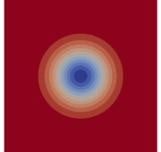
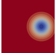
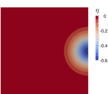
Fig. 1: The moving vortex test case: time evolution of the free surface elevation $\eta$ at times $t=0$, $t=1$ and $t=2$ computed using the ARS3 HDG-DG. The contour levels are from $-0.6$m to $0$m with the step-size of $0.05$m.

We compute the errors of the free surface elevation and the velocity using the following $L_{1}$, $L_{2}$ and $L_{\infty}$ norms:

$$L_{1}(q) :=\sum_{K\in{\Omega_{h}}}\int_{K}\left\lvert q-q_{T}\right\rvert dK,$$

$$L_{2}(q) :=\sqrt{\sum_{K\in{\Omega_{h}}}\int_{K}(q-q_{T})^{2}dK},$$

$$L_{\infty}(q) :=\max_{{q\in\Omega_{h}}}\left\lvert q-q_{T}\right\rvert,$$

where $q_{T}$ is the exact solution at the final time $T$.

For the spatial convergence test, we use the ARS3 HDG-DG scheme and take $\triangle t=0.000625$ for $p=5$, $\triangle t=0.00125$ for $p=4$, $\triangle t=0.0025$ for $p=3$ and $\triangle t=0.005$ for $p=2$. The errors are computed at $T=2$ when the center of the vortex reaches the right boundary of the domain. Table 1 shows the spatial convergence results using the $L_{1},L_{2}$ and $L_{\infty}$ norms for the free surface elevation $\eta$. As can be seen, the predicted convergence rate of $\left(p+1/2\right)$ is observed for all cases except for the case $p=5$ in which superconvergence is observed. In Table 2, similar convergence rates are observed for the $L_{2}$ errors of the horizontal velocity $(u,v)$ and the error in the energy norm $E:=\frac{1}{2}(\|\eta\|^{2}_{\Omega_{h}}+\|\mathbf{u}\|^{2}_{\Omega_{h}})$.

Table 1: Spatial convergence of $\eta$ for the traveling vortex test using ARS3 HDG-DG.

		Error			Order
$p$	$N_{e}$	$L_{1}$	$L_{2}$	$L_{\infty}$	$L_{1}$	$L_{2}$	$L_{\infty}$
2	4x4	2.036e-01	8.189e-02	3.372e-02	$-$	$-$	$-$
	8x8	4.455e-02	1.693e-02	8.623e-03	2.19	2.27	1.97
	16x16	6.561e-03	2.793e-03	2.083e-03	2.76	2.60	2.05
	32x32	1.057e-03	5.412e-04	4.269e-04	2.63	2.37	2.29
3	4x4	8.991e-02	3.645e-02	2.167e-02	$-$	$-$	$-$
	8x8	1.001e-02	4.226e-03	2.494e-03	3.17	3.11	3.12
	16x16	1.139e-03	5.864e-04	7.896e-04	3.14	2.85	1.66
	32x32	6.117e-05	3.228e-05	3.495e-05	4.22	4.18	4.50
4	4x4	1.999e-02	8.123e-03	6.767e-03	$-$	$-$	$-$
	8x8	1.287e-03	5.723e-04	6.756e-04	3.96	3.83	3.32
	16x16	5.053e-05	2.705e-05	3.020e-05	4.67	4.40	4.48
	32x32	2.244e-06	1.467e-06	1.273e-06	4.49	4.20	4.57
5	4x4	7.790e-03	3.015e-03	2.428e-03	$-$	$-$	$-$
	8x8	2.856e-04	1.408e-04	1.604e-04	4.77	4.42	3.92
	16x16	6.040e-06	3.378e-06	3.676e-06	5.56	5.38	5.45
	32x32	6.822e-08	4.193e-08	1.739e-08	6.47	6.33	7.72

Table 2: Spatial convergence of $\mathbf{u}$ and $\sqrt{E}$ for the traveling vortex test using ARS3 HDG-DG.

		$L_{2}$ Error			Order
$p$	$N_{e}$	$u$	$v$	$\sqrt{E}$	$u$	$v$	$\sqrt{E}$
2	4x4	1.654e-01	2.277e-01	2.072e-01	$-$	$-$	$-$
	8x8	4.993e-02	4.260e-02	4.793e-02	1.73	2.42	2.11
	16x16	1.196e-02	5.513e-03	9.517e-03	2.06	2.95	2.33
	32x32	2.534e-03	9.236e-04	1.945e-03	2.24	2.58	2.29
3	4x4	1.665e-01	8.503e-02	1.347e-01	$-$	$-$	$-$
	8x8	9.142e-03	5.988e-03	8.285e-03	4.19	3.83	4.02
	16x16	9.278e-04	7.128e-04	9.254e-04	3.30	3.07	3.16
	32x32	5.166e-05	4.479e-05	5.347e-05	4.17	3.99	4.11
4	4x4	1.734e-02	1.707e-02	1.814e-02	$-$	$-$	$-$
	8x8	1.199e-03	1.092e-03	1.216e-03	3.85	3.97	3.90
	16x16	5.942e-05	3.699e-05	5.306e-05	4.33	4.88	4.52
	32x32	3.593e-06	1.660e-06	2.985e-06	4.05	4.48	4.15
5	4x4	1.403e-02	6.759e-03	1.121e-02	$-$	$-$	$-$
	8x8	2.666e-04	1.623e-04	2.421e-04	5.72	5.38	5.53
	16x16	5.734e-06	3.357e-06	5.270e-06	5.54	5.60	5.52
	32x32	6.808e-08	4.744e-08	6.574e-08	6.40	6.14	6.32

To numerically compute the temporal convergence for ARS2 HDG-DG and ARS3 HDG-DG, we simulate the translational vortex with a $6th$-order solution on the $32\times 32$-element mesh. The time-step size $\triangle t$ varies from $10^{-4}$ to $5\times 10^{-3}$, which corresponds to Courant numbers from $0.11$ to $5.6$. We compute the error at $T=0.1$. The mean water depth $H_{\infty}$ is set to be $50$ so that the reference Froude number, $Fr=\frac{u_{\infty}}{\sqrt{gH_{\infty}}}$, is $0.1$, that is, the gravity wave dominates the convection. In Figure 2(a), we observe the correct second-order and third-order convergence in time for ARS2 HDG-DG and ARS3 HDG-DG, respectively. To demonstrate the stability benefit of the IMEX HDG-DG scheme we perform simulations for a wide range of Courant numbers (Cr) from $0.28$ (the point over which the second order RKDG, denoted as RK2 DG, blows up) to $5.6$.

Clearly, the IMEX HDG-DG approaches are more economical than our previous work on IMEX DG [20, 19] due to the fewer number of coupled degrees of freedom. Compared to standard fully implicit methods, they are much more advantageous since only one linear solve is needed for each stage per time-step. For this paper, our methods are in fact “optimal” in the sense that the HDG matrix in (52), and hence the matrices $\mathbf{A}$ in (53) and $\left(\mathbf{D}-\mathbf{C}\mathbf{A}^{-1}\mathbf{B}\right)$ in (54), is the same for any time-step and any stage (since $\tilde{a}_{ii}$ are the same at any stage for the chosen schemes). Thus, we need to perform the LU factorization (here we use UMFPACK [14]) of the HDG-trace matrix $\left(\mathbf{D}-\mathbf{C}\mathbf{A}^{-1}\mathbf{B}\right)$ once, and the same LU factors can be recycled (via a forward substitution followed by a backward substitution) for all subsequent computations involving (54).

Clearly, our approaches cannot compete with fully explicit methods in terms of wallclock time since we still have to solve (53) and (54) for each time-step. To demonstrate this we plot in Figure 2(b) the $L^{2}$ error of the free surface height against the wallclock time for ARS2 HDG-DG, ARS3 HDG-DG, RK2 DG, and RK3 DG (the third order RKDG). To improve the wallclock time we can, for example, develop iterative solvers for (54) and solve (53); this will be presented in our future work. Nevertheless, for applications in which fast time marching to the solution is more important than an accurate solution, our methods are more advantageous than the fully explicit counterparts due to their ability to take (much) larger time-step sizes: we will confirm this claim in section 6.2.

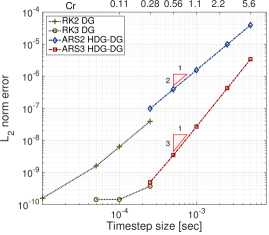
(a) Accuracy/Stability

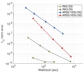
(b) Wallclock time

Fig. 2: Comparison between IMEX HDG-DG and RKDG for the moving vortex test case: (a) the accuracy/stability and (b) the wallclock time.

6.2 Water height perturbation

In this section, we consider the propagation of smooth gravity waves [15] over the domain $\Omega=[-1,1]\times[-1,1]$. The initial condition is given as

$$H=H_{\infty}+e^{-\frac{x^{2}+y^{2}}{2\sigma^{2}}},\quad\text{ and }\quad u=v=0,$$

where $H_{\infty}=100$. We set the gravitational acceleration $g$ to be unity. The domain is discretized with $20\times 20$ finite elements and with $8th$ order polynomials. The time horizon is $T=0.16$.

We choose different time-step sizes for RK2 DG and ARS2 HDG-DG. Since RK2 DG blows up after a few iterations with $\triangle t$=0.0002 (see Figure 3), we take $\triangle t=0.0001$. The time-step sizes of $\triangle t=0.002$ and $\triangle t=0.02$ are chosen for ARS2 HDG-DG. Figure 4 quantitatively shows a three-dimensional plot of the evolution of the free surface elevation using RK2 DG and ARS2 HDG-DG at times $t=0$, $t=0.02$, $t=0.06$, and $t=0.1$. We observe that ARS2 HDG-DG with $\triangle t=0.002$ is in good agreement with RK2 DG. While IMEX-RK methods allow us to increase the time-step size without being penalized by stability constraints their accuracy is reduced due to the truncation error in the time discretization. This can be observed in the last column of Figure 4 in which ARS2 HDG-DG with $\triangle t=0.02$ shows damped (inaccurate) solutions due to large truncation error.

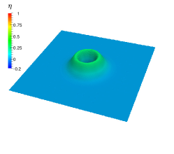
(a) T=0.016

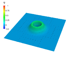
(b) T=0.017

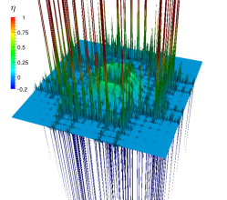
(c) T=0.018

Fig. 3: Water height perturbation test: free surface evolution for RK2 DG ($\triangle t$=0.0002) at $t=0.016$, $t=0.017$ and $t=0.018$.

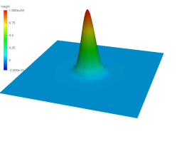
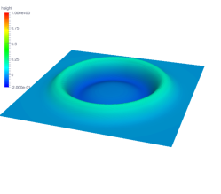
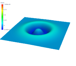
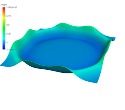
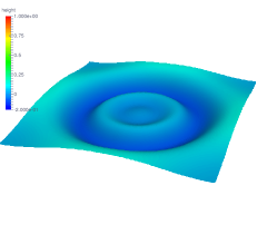
Fig. 4: Water height perturbation test: free surface evolution for RK2 DG ($\triangle t$=0.0001, left), ARS2 HDG-DG ($\triangle t$=0.002, center) and ARS2 HDG-DG ($\triangle t$=0.02, right) at times $t=0$, $t=0.06$, and $t=0.1$.

In Table 3, we compare the wallclock times of ARS2 HDG-DG with those of RK2 DG. As can be seen, ARS2 HDG-DG with $\triangle t=0.002$ is comparable to RK2 DG with $\triangle t=0.0001$ in both wallclock time and in accuracy (see Figure 4). When $\triangle t=0.02$ (two hundred times larger than RK2 DG stable time-step size), ARS2 HDG-DG outperforms RK2 DG in terms of computational cost (though with a less accurate solution).

Table 3: Water height perturbation test: wallclock time comparison for ARS2 HDG-DG and RK2 DG where TI denotes time-integrator.

TI	$\triangle t$	Cr	Wallclock time
RK2 DG	0.0001	0.2	18m 20s
ARS2 HDG-DG	0.0020	4.0	20m 41s
ARS2 HDG-DG	0.0200	40.0	2m 28s

6.3 Steady-state geostrophic flow

We consider the steady-state geostrophic flow in [51] (a geostrophically balanced flow). This flow admits an analytical solution for the shallow water equations on the sphere [34]. The initial condition is given by

$$H =H_{\infty}-\frac{1}{g}\left(a\Omega+\frac{u_{\infty}^{2}}{2}\right)\cos^{2}\theta,$$ (56a)

$$u_{\lambda} =u_{\infty}\cos\theta,$$ (56b)

$$u_{\theta} =0,$$ (56c)

where $(u_{\lambda},u_{\theta})$ is the local tangential velocity in latitude-longitude coordinates $(\lambda,\theta)$. We take $gH_{\infty}=2.94\times 10^{4}m^{2}s^{-2}$, and $u_{\infty}=38.61ms^{-1}$. The numerical experiment is performed on a grid with $N_{e}=1536$ elements ($16\times 16$ elements on each of the six faces of the cubed-sphere) and solution order $p=4$. The time-step size for ARS2 HDG-DG is $864s$.

Figure 5 shows the snapshot of the height field from the ARS2 HDG-DG approach (Figure 5(a)) and the exact field (Figure 5(b)) after $12$ days. The height field from ARS2 HDG-DG is almost the same as the exact solution. Indeed, we show in Figure 5(c) the relative error of the height field, $|\frac{H_{num}-H_{exact}}{H_{exact}}|$, and the maximum relative error of $\mathcal{O}\left(10^{-7}\right)$ is observed (see also Figure 6(a)).

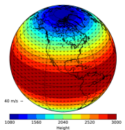
(a) ARS2 HDG-DG

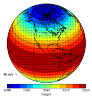
(b) Exact solution

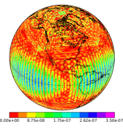
(c) Relative error

Fig. 5: Geostrophic flow test case: (a) total height field from ARS2 HDG-DG at day 12 with Cr $=1.36$, (b) the exact solution, and (c) the relative error of the height field.

Figure 6 shows the time series of the height field error, mass, and energy loss in $L_{1}$, $L_{2}$ and $L_{\infty}$ norms.

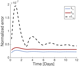
(a) Height errors in $L_{1}$, $L_{2}$ and $L_{\infty}$ norms

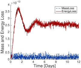
(b) Mass and energy loss

Fig. 6: Geostrophic flow test case: (a) time evolution of height field error in $L_{1}$, $L_{2}$ and $L_{\infty}$ norms, and (b) mass and energy loss of the ARS2 HDG-DG solution with time-step size of $864\text{s}$ (i.e. Cr $=1.36$).

Here, the mass and energy losses are defined as

$$\text{ mass loss }=\left\lvert\frac{\text{mass}(t)-\text{mass}(0)}{\text{mass}(0)}\right\rvert,\text{ energy loss }=\left\lvert\frac{\text{energy}(t)-\text{energy}(0)}{\text{energy}(0)}\right\rvert,$$

where $\text{mass}:=\|H\|^{2}_{\Omega_{h}}$ and $\text{energy}:=\|H\mathbf{u}\cdot\mathbf{u}+gH^{2}\|^{2}_{\Omega_{h}}$. We observe the energy and mass are conserved and this is a direct consequence of the fact that both DG and HDG are conservative discretizations.

6.4 Steady-state geostrophic flow with compact support

This case is similar to the steady-state geostrophic flow in section 6.3. The difference is that it is equipped with a compactly supported wind field, considered as a high latitude jet in the northern hemisphere. The initial condition is given as

$$H =H_{\infty}-\frac{a}{g}\int_{-\pi/2}^{\theta}\left(f+\frac{u(\tau)\tan\tau}{a}\right)u(\tau)d\tau,$$ (57a)

$$u_{\lambda} =u_{\infty}b(x)b(x_{e}-x)e^{4/x_{e}},$$ (57b)

$$u_{\theta} =0,$$ (57c)

where $\theta_{b}=-\pi/6$, $\theta_{e}=\pi/2$, $x_{e}=0.3$, $x=x_{e}\frac{\theta-\theta_{b}}{\theta_{e}-\theta_{b}},$ and $b(x)=\begin{cases}0&\text{for }x\leq 0,\\ e^{-1/x}&\text{for }0<x.\end{cases}$

The total simulation time is 12 days. As shown in Figure 7, the height field of the ARS2 HDG-DG solution is similar to that of the exact solution: indeed Figure 7(c) shows that the relative error is of order $\mathcal{O}\left(10^{-5}\right)$.

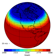
(a) ARS2 HDG-DG

(b) Exact solution

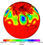
(c) Relative error

Fig. 7: Steady-state geostrophic flow with compact support: (a) total height field from ARS2 HDG-DG at day 12 with Cr $=1.2$, (b) the exact solution, and (c) the relative error of the height field.

For the spatial convergence test, we conduct both $h$-convergence and $p$-convergence studies in Figure 8.

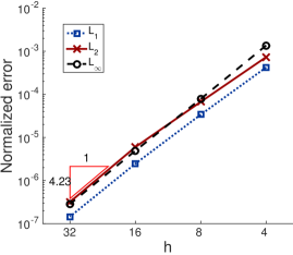
(a) h-convergence

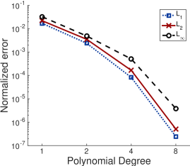
(b) p-convergence

Fig. 8: Convergence studies for the ARS2 HDG-DG scheme when applied to the steady-state geostrophic flow with compact support with Cr $=0.7$: (a) $\mathrm{h}$-convergence with $p=3$ and (b) $p$-convergence with $N_{e}=6144$.

The errors are measured at $T=0.4$ with Cr $=0.7$. For $h$-convergence, the height field error in $L_{1}$, $L_{2}$ and $L_{\infty}$ norms are computed for $p=3$ and the total number of elements is given by $N_{e}=6{\mathrm{n}}^{2}$, where ${\mathrm{n}}=\left\{4,8,16,32\right\}$. As can be seen in Figure 8(a), the convergence rate is $p+1$. For $p$-convergence, an exponential rate is observed in Figure 8(b).

6.5 Zonal flow over an isolated mountain

We consider the zonal flow over an isolated mountain test proposed in [51]. The height and wind fields are similar to those of the steady-state geostrophic flow, but now $H_{\infty}=5960\text{m}$ and $u_{\infty}=20\text{ms}^{-1}$. A mountain with height $H_{s}=2000(1-r/r_{s})\text{m}$, located at $(\lambda_{c},\theta_{c})=(3\pi/2,\pi/6)$, is introduced in the flow, where $r_{s}=\frac{\pi}{9}$ and $r^{2}=\min(r^{2},(\lambda-\lambda_{c})^{2}+(\theta-\theta_{c})^{2})$.

We plot the height field at days 5, 10 and 15 in Figure 9 on a grid with $N_{e}=384$ elements ($8\times 8\times 6$ elements on the cubed-sphere) and solution order $p=8$. The time-step size of 432 seconds is taken. As can be seen, the height fields are smooth and comparable to the corresponding results in [34, 47] (note that this problem has no analytical solution).

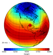
(a) Day 5

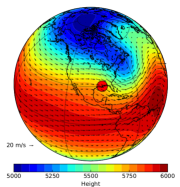
(b) Day 10

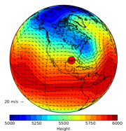
(c) Day 15

Fig. 9: Flow over an isolated mountain (red circle) computed with the ARS2 HDG-DG scheme: shown are the total water height after (a) 5 days, (b) 10 days, and (c) 15 days. The numerical experiments are performed on a grid with $N_{e}=384$ elements, solution order $p=8$, and Cr $=1.2$. Contour levels are from $5000$m to $6000$m with 21 levels.

We compare the height field of ARS2 HDG-DG with that of RK2 DG in Figure 10. We take $\triangle t=43.2$ seconds (Cr=0.15) for RK2 DG. The height field of ARS2 HDG-DG is in good agreement with that of RK2 DG: the relative difference in the height field is $\mathcal{O}\left(10^{-3}\right)$.

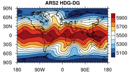
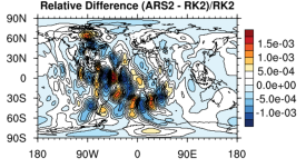
Fig. 10: The zonal flow over an isolated mountain: total height field computed from ARS2 HDG-DG (left) at day 15 with Cr of $1.46$; the relative difference (right) with RK2 in the height field.

6.6 Rossby-Haurwitz wave

We next consider the Rossby-Haurwitz wave test in [51]. The Rossby-Haurwitz wave is an exact solution of the nonlinear barotropic vorticity equation [24], but not an exact solution of the shallow water system [34]. The wave number is chosen to be 4.

To simulate this test case, we use the ARS2 HDG-DG scheme on a grid with $N_{e}=864$ elements ($12\times 12\times 6$), solution order $p=5$, and with a time-step size of 345.6 seconds (i.e. Cr$=1.2$). The height fields at days 0, 7 and 14 are shown in Figure 11. We also compare the results of ARS2 HDG-DG with those of RK2 DG in Figure 12 after 14 days. For RK2 DG, we take the time-step size to be $43.2$ seconds (Cr=$0.14$) for stability. The height field of ARS2 HDG-DG is in good agreement with that of RK2 DG. In particular, the relative difference in the height field is $\mathcal{O}\left(10^{-3}\right)$.

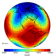
(a) Day 0

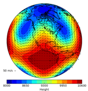
(b) Day 7

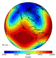
(c) Day 14

Fig. 11: Rossby-Haurwitz wave: the total height field computed from ARS2 HDG-DG after a) 0 days, (b) 7 days, and (c) 14 days. The numerical experiment is performed on the grid with $N_{e}=864$ elements, solution order $p=5$, and Cr $=1.2$. Contour levels are from $8000$m to $10600$m with the step size of $173$m.

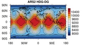
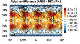
Fig. 12: Rossby-Haurwitz wave: the total height field computed from ARS2 HDG-DG (left) after 14 days with Cr of $1.2$; the relative difference (right) with RK2 in the height field.

6.7 Barotropic instability test

In this section, we consider the barotropic instability test in [17]. A zonal jet, a wind field along a latitude line and geostrophically balanced height field, is initialized in the northern hemisphere. Then, the height field is perturbed by adding a smoothly localized bump to the center of the jet, which causes barotropic waves to evolve in time. Figure 13 shows the relative vorticity field of the barotropically unstable flow at days 4, 5 and 6. The numerical experiment is conducted on the grid with $N_{e}=5400$ elements ($30\times 30\times 6$), solution order $p=4$, and time-step size of $173$ seconds. The vorticity field computed from ARS2 HDG-DG is comparable to that of [32], which use high-order continuous and discontinuous Galerkin methods with explicit time-integration.

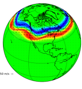
(a) Day 4

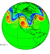
(b) Day 5

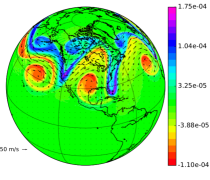
(c) Day 6

Fig. 13: Barotropic instability test: relative vorticity field of the ARS2 HDG-DG at (a) 4 days, (b) 5 days, and (c) 6 days. The numerical experiment was performed on the grid of $N_{e}=5400$ and $p=4$ with a time-step size of 173 seconds (Cr=0.94). The vorticity ranges from $-1.1\times 10^{-4}$ to $1.75\times 10^{4}$.

We also compare the results of ARS2 HDG-DG with those of RK2 DG in Figure 14 after 6 days. For RK2 DG, we take the time-step size to be $21.6$ seconds (i.e Cr =$0.12$) for stability. The vorticity field of ARS2 HDG-DG is in good agreement with that of RK2 DG. Indeed, the difference in the vorticity field is $O(10^{-6})$.

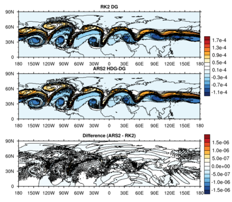
Fig. 14: Barotropic instability test: relative vorticity fields of RK2 DG (top) and ARS2 HDG-DG (middle) at 6 days with Cr of $0.94$ and $0.12$, respectively; the difference (bottom) in the vorticity field between ARS2 HDG-DG and RK2 DG.

7 Conclusions

In this paper, we are interested in subcritical shallow water systems in which gravity wave velocity is faster than convection speed. We start by decomposing the original flux into a linear part (obtained from linearizing the flux at the lake at rest condition) containing the fast gravity wave and a nonlinear part for which the fastest wave is removed. We spatially discretize the former using an HDG method, and the latter using a DG approach. This enables us to develop an IMEX HDG-DG framework in which we integrate the DG discretization explicitly and the HDG discretization implicitly. The purpose of our coupled approach is fourfold: (i) to step over the fast waves using larger time step sizes (compared to fully explicit methods) without facing instability; (ii) to avoid expensive Newton-type iterations (compared to fully implicit methods) for each time step; (iii) to take advantage of the DOF reduction in HDG method (relative to DG approaches) to further reduce the cost of linear solves; and (iv) to preserve high-order accuracy in both space and time.

Numerical results have shown that while fully explicit DG approaches are stable with small time-step sizes, our IMEX HDG-DG method is stable for orders of magnitude larger time-step sizes. We have shown that only one forward and one backward substitutions are required for each stage per time-step. The numerical results also show that our approach achieves the expected high-order accuracy both in space and time. Ongoing work is to further improve the efficiency of the IMEX HDG-DG approach by developing preconditioned iterative methods for the linear solve, and to implement the scheme on parallel computing systems. Future developments also include construction of IMEX HDG-DG approach for nonhydrostatic equations (stratified compressible Euler/Navier-Stokes systems) where it is expected that our approach will yield greater benefits due to the stiffness of the acoustic waves (waves that carry little energy yet dominate the time-step restriction). Of interest will be the rigorous convergence analysis of the IMEX-HDG-DG scheme. Due to the similarity between the weak Galerkin methods [48, 49] and HDGs, our ongoing work is to extend the IMEX idea to the weak Galerkin framework.

References

- [1] V. Aizinger and C. Dawson, A discontinuous Galerkin method for two-dimensional flow and transport in shallow water, Advances in Water Resources, 25 (2002), pp. 67–84.
- [2] Uri M Ascher, Steven J Ruuth, and Raymond J Spiteri, Implicit-explicit runge-kutta methods for time-dependent partial differential equations, Applied Numerical Mathematics, 25 (1997), pp. 151–167.
- [3] Ivo Babuvska and Manil Suri, The -version of the finite element method with quasiuniform meshes, Mathematical Modeling and Numerical Analysis, 21 (1987), pp. 199–238.
- [4] , The and - version of the finite element method, basic principles and properties, SIAM Review, 36 (1994), pp. 578–632.
- [5] Sébastien Blaise, Jonathan Lambrechts, and Eric Deleersnijder, A stabilization for three-dimensional discontinuous galerkin discretizations applied to nonhydrostatic atmospheric simulations, International Journal for Numerical Methods in Fluids, (2015).
- [6] T. Bui-Thanh, From Godunov to a unified hybridized discontinuous Galerkin framework for partial differential equations, Journal of Computational Physics, 295 (2015), pp. 114–146.
- [7] Tan Bui-Thanh, Construction and analysis of hdg methods for linearized shallow water equations, SIAM Journal on Scientific Computing, 38 (2016), pp. A3696–A3719.
- [8] B. Cockburn, B. Dong, J. Guzman, M. Restelli, and R. Sacco, A hybridizable discontinuous Galerkin method for steady state convection-diffusion-reaction problems, SIAM J. Sci. Comput., 31 (2009), pp. 3827–3846.
- [9] B. Cockburn and J. Gopalakrishnan, The derivation of hybridizable discontinuous Galerkin methods for Stokes flow, SIAM J. Numer. Anal, 47 (2009), pp. 1092–1125.
- [10] Bernardo Cockburn, Jay Gopalakrishnan, and Raytcho Lazarov, Unified hybridization of discontinuous Galerkin, mixed, and continuous Galerkin methods for second order elliptic problems, SIAM J. Numer. Anal., 47 (2009), pp. 1319–1365.
- [11] B. Cockburn, F. Li, N. C. Nguyen, and J. Peraire, Hybridization and postprocessing techniques for mixed eigenfunctions, SIAM J. Numer. Anal, 48 (2010), pp. 857–881.
- [12] Bernardo Cockburn and Chi-Wang Shu, The runge–kutta discontinuous galerkin method for conservation laws v: multidimensional systems, Journal of Computational Physics, 141 (1998), pp. 199–224.
- [13] J Côté, A lagrange multiplier approach for the metric terms of semi-lagrangian models on the sphere, Quarterly Journal of the Royal Meteorological Society, 114 (1988), pp. 1347–1352.
- [14] Timothy A Davis, Direct methods for sparse linear systems, SIAM, 2006.
- [15] M. Dumbser and V. Casulli, A staggered semi-implicit spectral discontinuous Galerkin scheme for the shallow water equations, Applied Mathematics and Computation, 219 (2013), pp. 8057–8077.
- [16] M. Feistauer, V. Dolejsi, and V. Kucera, On the discontinuous Galerkin method for the simulation of compressible flow with wide range of Mach numbers, Computing and Visualization in Science, 10 (2007), pp. 17–27.
- [17] Joseph Galewsky, Richard K Scott, and Lorenzo M Polvani, An initial-value problem for testing numerical models of the global shallow-water equations, Tellus A, 56 (2004), pp. 429–440.
- [18] Francis X Giraldo, Jan S Hesthaven, and Tim Warburton, Nodal high-order discontinuous galerkin methods for the spherical shallow water equations, Journal of Computational Physics, 181 (2002), pp. 499–525.
- [19] Francis X Giraldo, James F Kelly, and EM Constantinescu, Implicit-explicit formulations of a three-dimensional nonhydrostatic unified model of the atmosphere (numa), SIAM Journal on Scientific Computing, 35 (2013), pp. B1162–B1194.
- [20] F. X. Giraldo and M. Restelli, High-order semi-implicit time-integrators for a triangular discontinous Galerkin oceanic shallow water model, International Journal For Numerical Methods In Fluids, 63 (2010), pp. 1077–1102.
- [21] F. X. Giraldo and T. Warburton, A high-order triangular discontinous Galerkin oceanic shallow water model, International Journal For Numerical Methods In Fluids, 56 (2008), pp. 899–925.
- [22] Sylvie Gravel and Andrew Staniforth, A mass-conserving semi-lagrangian scheme for the shallow-water equations, Monthly Weather Review, 122 (1994), pp. 243–248.
- [23] R. Griesmaier and P. Monk, Error analysis for a hybridizable discontinous Galerkin method for the Helmholtz equation, J. Sci. Comput., 49 (2011), pp. 291–310.
- [24] Bernhard Haurwitz, The motion of atmospheric disturbances on the spherical earth, J. mar. Res, 3 (1940), pp. 254–267.
- [25] Jan S Hesthaven and Tim Warburton, Nodal discontinuous Galerkin methods: algorithms, analysis, and applications, Springer Science & Business Media, 2007.
- [26] Christopher A Kennedy and Mark H Carpenter, Additive runge-kutta schemes for convection-diffusion-reaction equations, Applied Numerical Mathematics, 44 (2003), pp. 139–181.
- [27] R. M. Kirby, S. J. Sherwin, and B. Cockburn, To CG or to HDG: A comparative study, J. Sci. Comput., 51 (2012), pp. 183–212.
- [28] Matthias Läuter, Francis X Giraldo, Dörthe Handorf, and Klaus Dethloff, A discontinuous galerkin method for the shallow water equations in spherical triangular coordinates, Journal of Computational Physics, 227 (2008), pp. 10226–10242.
- [29] Randall J LeVeque, Finite volume methods for hyperbolic problems, vol. 31, Cambridge university press, 2002.
- [30] H. Li and R. X. Liu, The discontinuous Galerkin finite element method for the 2D shallow water equations, Mathematics and Computers in Simulation, 56 (2001), pp. 171–184.
- [31] L. Li, S. Lanteri, and R. Perrrussel, A hybridizable discontinuous Galerkin method for solving 3D time harmonic Maxwell’s equations, in Numerical Mathematics and Advanced Applications 2011, Springer, 2013, pp. 119–128.
- [32] S Marras, Michal A Kopera, and Francis X Giraldo, Simulation of shallow-water jets with a unified element-based continuous/discontinuous galerkin model with grid flexibility on the sphere, Quarterly Journal of the Royal Meteorological Society, 141 (2015), pp. 1727–1739.
- [33] D. Moro, N. C. Nguyen, and J. Peraire, Navier-Stokes solution using hybridizable discontinuous Galerkin methods, American Institute of Aeronautics and Astronautics, 2011-3407 (2011).
- [34] Ramachandran D Nair, Stephen J Thomas, and Richard D Loft, A discontinuous galerkin global shallow water model, Monthly weather review, 133 (2005), pp. 876–888.
- [35] N. C. Nguyen, J. Peraire, and B. Cockburn, An implicit high-order hybridizable discontinuous Galerkin method for linear convection-diffusion equations, Journal Computational Physics, 228 (2009), pp. 3232–3254.
- [36] , An implicit high-order hybridizable discontinuous Galerkin method for nonlinear convection-diffusion equations, Journal Computational Physics, 228 (2009), pp. 8841–8855.
- [37] , A hybridizable discontinous Galerkin method for Stokes flow, Comput Method Appl. Mech. Eng., 199 (2010), pp. 582–597.
- [38] , High-order implicit hybridizable discontinuous Galerkin method for acoustics and elastodynamics, Journal Computational Physics, 230 (2011), pp. 3695–3718.
- [39] , An implicit high-order hybridizable discontinuous Galerkin method for the incompressible Navier-Stokes equations, Journal Computational Physics, 230 (2011), pp. 1147–1170.
- [40] Lorenzo Pareschi and Giovanni Russo, Implicit-explicit runge-kutta schemes and applications to hyperbolic systems with relaxation, Journal of Scientific computing, 25 (2005), pp. 129–155.
- [41] M. Restelli and F. X. Giraldo, A conservative discontinuous Galerkin semi-implicit formulation for the Navier-Stokes equations in non-hydrostatic mesoscale modeling, SIAM Journal on Scientific Computing, 31 (2009), pp. 2231–2257.
- [42] Mario Ricchiuto and Andreas Bollermann, Stabilized residual distribution for shallow water simulations, Journal of Computational Physics, 228 (2009), pp. 1071–1115.
- [43] Béatrice Rivière and Mary F Wheeler, A discontinuous galerkin method applied to nonlinear parabolic equations, in Discontinuous Galerkin methods, Springer, 2000, pp. 231–244.
- [44] P. L. Roe, Approximate riemann solvers, parametric vectors, and difference schemes, Journal of Computational Physics, 43 (1981), pp. 357–372.
- [45] Vladimir Vasil’evich Rusanov, The calculation of the interaction of non-stationary shock waves and obstacles, USSR Computational Mathematics and Mathematical Physics, 1 (1962), pp. 304–320.
- [46] Eleuterio F Toro, Riemann problems and the waf method for solving the two-dimensional shallow water equations, Philosophical Transactions of the Royal Society of London A: Mathematical, Physical and Engineering Sciences, 338 (1992), pp. 43–68.
- [47] Paul A Ullrich, Christiane Jablonowski, and Bram Van Leer, High-order finite-volume methods for the shallow-water equations on the sphere, Journal of Computational Physics, 229 (2010), pp. 6104–6134.
- [48] Junping Wang and Xiu Ye, A weak galerkin finite element method for second-order elliptic problems, Journal of Computational and Applied Mathematics, 241 (2013), pp. 103–115.
- [49] , A weak galerkin mixed finite element method for second order elliptic problems, Mathematics of Computation, 83 (2014), pp. 2101–2126.
- [50] Hilary Weller, Sarah-Jane Lock, and Nigel Wood, Runge–kutta imex schemes for the horizontally explicit/vertically implicit (hevi) solution of wave equations, Journal of Computational Physics, 252 (2013), pp. 365–381.
- [51] David L Williamson, John B Drake, James J Hack, Rüdiger Jakob, and Paul N Swarztrauber, A standard test set for numerical approximations to the shallow water equations in spherical geometry, Journal of Computational Physics, 102 (1992), pp. 211–224.
- [52] Yan Xu and Chi-wang Shu, Local discontinuous galerkin methods for three classes of nonlinear wave equations, Journal of Computational Mathematics, (2004), pp. 250–274.