Atypical energy eigenstates in the Hubbard chain and quantum disentangled liquids

Abstract

We investigate the implications of integrability for the existence of quantum disentangled liquid (QDL) states in the half-filled one-dimensional Hubbard model. We argue that there exist finite energy-density eigenstates that exhibit QDL behaviour in the sense of J. Stat. Mech. P10010 (2014). These states are atypical in the sense that their entropy density is smaller than that of thermal states at the same energy density. Furthermore, we show that thermal states in a particular temperature window exhibit a weaker form of the QDL property, in agreement with recent results obtained by strong-coupling expansion methods in arXiv:1611.02075. This article is part of the themed issue ‘Breakdown of ergodicity in quantum systems: from solids to synthetics matter’.

I Introduction

The question of how isolated many-particle quantum systems relax and how to describe their steady state behaviour has attracted attention for a long timevonNeumann . The past decade has witnessed a tremendous resurgence of interest in this problem, which was largely motivated by ground-breaking experiments on systems of trapped ultra-cold atomsGM:col_rev02 ; kww-06 ; HL:Bose07 ; hacker10 ; tetal-11 ; getal-11 ; cetal-12 ; langen13 ; MM:Ising13 ; zoran1 ; MBLex1 . It is now understood that generic many-body systems relax towards thermal equilibrium distributions at an effective temperature fixed by the energy density, which is, by definition, conserved for isolated systems. This behaviour follows from the eigenstate thermalisation hypothesis (ETH)Deutsch91 ; Sred1 ; Sred2 ; ETH . When a system thermalises the only information about the initial state that is retained at late times is its energy density. This does not, however, exhaust the theoretically understood paradigms of relaxation: quantum integrable systems possess conservation laws that constrain the system to retain information on more than just the energy density. As such, they do not thermalise, but instead relax towards Generalised Gibbs Ensembles GGE ; cc-07 ; EFreview ; Cazalilla ; VR ; GGE_int . This can be understood in terms of a generalised ETHGETH ; CE13 . Sufficiently strong disorder is another mechanism that can preclude thermalisationMBL1 ; MBL2 ; MBL3 ; MBL4 ; MBL5 ; MBL6 . This can again be related to the existence of conservation lawsMBL6 ; MBL7 ; MBL8 , although, unlike in the integrable case, no fine-tuning is required. Moreover, in (many-body) localised systems eigenstates at finite energy densities exhibit an area-law scaling of the entanglement entropy (EE). This is qualitatively different to cases in which the ETH holds and differs dramatically from the situation encountered in integrable models.

Recently it has been proposed that the eigenstates of certain systems may fail to thermalise in the conventional sense. The corresponding state of matter has been dubbed the “quantum disentangled liquid” (QDL)qdl . A characteristic feature of such systems is that they comprise both heavy and light degrees of freedom. The basic premise of the QDL concept is that, while the heavy degrees of freedom are fully thermalised, the light ones, which are enslaved to the heavy particles, are not independently thermalised. A convenient diagnostic for such a state of matter is the bipartite EE after a projective measurement of the heavy particles. The possibility of realising a QDL in the one-dimensional Hubbard model was subsequently investigated by exact diagonalisation of small systems in Ref. hubb1, . Given the limitations on accessible system sizes it is difficult to draw definite conclusions from these results. Motivated by these studies we have recently explored the possibility of realising a QDL in the half-filled Hubbard model on bipartite lattices by analytic meansQDLHubbard . Here we provide additional details regarding the integrability-based approach put forward in that work. The Hamiltonian of the one-dimensional Hubbard model is

$$H=-t\sum_{j,\sigma=\uparrow,\downarrow}\left(c^{\dagger}_{j,\sigma}c^{\phantom{\dagger}}_{j+1,\sigma}+c^{\dagger}_{j+1,\sigma}c^{\phantom{\dagger}}_{j,\sigma}\right)+U\sum_{j}\big{(}n_{j,\uparrow}-\frac{1}{2}\big{)}\big{(}n_{j,\downarrow}-\frac{1}{2}\big{)}.$$ (1)

Here $c^{\phantom{\dagger}}_{j,\sigma}$, $c^{\dagger}_{j,\sigma}$ are fermionic operators satisfying the usual anticommutation relations, $n_{j,\sigma}=c^{\dagger}_{j,\sigma}c^{\phantom{\dagger}}_{j,\sigma}$, $t>0$ is the hopping parameter and $U>0$ is the strength of the on-site repulsion.

The outline of this paper is as follows. In Section II we briefly recall necessary facts from the exact solution of the Hubbard model. In Section III we consider typical states at finite temperature. In Sections IVand V we employ methods of integrability to show that it is possible to construct particular eigenstates at finite energy densities for which the charge degrees of freedom do not contribute to the volume term in the bipartite EE, corroborating the notion of the QDL diagnostic proposed in Ref. qdl, . In Section VI we show that there exists a parametrically large regime in which thermal states support a weaker version of QDL as proposed in Ref. QDLHubbard, .

II Eigenstates of the Hubbard Hamiltonian

The Bethe Ansatz method provides an exact solution of the one-dimensional Hubbard modelbook . Within the framework of the string hypothesis, eigenstates in the Hubbard model are determined by solutions to Takahashi’s equationsbook . For a state with $N$ electrons, $M$ of which are spin-down, they read

$$\frac{2\pi I_{j}}{L} =k_{j}+\frac{1}{L}\sum_{n=1}^{\infty}\sum_{\alpha=1}^{M_{n}}\theta\left(\frac{\sin k_{j}-\Lambda^{n}_{\alpha}}{nu}\right)+\frac{1}{L}\sum_{n=1}^{\infty}\sum_{\alpha=1}^{M_{n}^{\prime}}\theta\left(\frac{\sin k_{j}-{\Lambda^{\prime}}_{\alpha}^{n}}{nu}\right), \qquad j=1,\dots,N-2M^{\prime},$$

$$\frac{2\pi J^{n}_{\alpha}}{L} =\frac{1}{L}\sum_{j=1}^{N-2M^{\prime}}\theta\left(\frac{\Lambda^{n}_{\alpha}-\sin k_{j}}{nu}\right)-\frac{1}{L}\sum_{m=1}^{\infty}\sum_{\beta=1}^{M_{m}}\Theta_{nm}\left(\frac{\Lambda^{n}_{\alpha}-\Lambda^{m}_{\beta}}{u}\right), \qquad\alpha=1,\dots,M_{n},$$

$$\frac{2\pi{J^{\prime}}^{n}_{\alpha}}{L} =-\frac{1}{L}\sum_{j=1}^{N-2M^{\prime}}\theta\left(\frac{{\Lambda^{\prime}}^{n}_{\alpha}-\sin k_{j}}{nu}\right)-\frac{1}{L}\sum_{m=1}^{\infty}\sum_{\beta=1}^{M^{\prime}_{m}}\Theta_{nm}\left(\frac{{\Lambda^{\prime}}^{n}_{\alpha}-{\Lambda^{\prime}}^{m}_{\beta}}{u}\right)$$

$$+2{\rm Re}[\arcsin({\Lambda^{\prime}}^{n}_{\alpha}+niu)], \qquad\alpha=1,\dots,M_{n}^{\prime},$$

where $u=U/4t$, $\theta(x)=2\arctan(x)$,

$$\Theta_{nm}(x)=\begin{cases}\theta\left(\frac{x}{|n-m|}\right)+2\theta\left(\frac{x}{|n-m|+2}\right)+\dots+2\theta\left(\frac{x}{n+m-2}\right)+\theta\left(\frac{x}{n+m}\right),&n\neq m\\ 2\theta\left(\frac{x}{2}\right)+2\theta\left(\frac{x}{4}\right)+\dots+2\theta\left(\frac{x}{2n-2}\right)+\theta\left(\frac{x}{2n}\right),&n=m\end{cases},$$ (2)

and

$$M=\sum_{n=1}^{\infty}n(M_{n}+M_{n}^{\prime}),\qquad M^{\prime}=\sum_{n=1}^{\infty}nM_{n}^{\prime}.$$ (3)

The sets $\{I_{j}\}$, $\{J^{n}_{\alpha}\}$, $\{{J^{\prime}}^{n}_{\alpha}\}$ of integer or half-odd integer numbers specify the particular eigenstate under consideration and obey the “selection rules”

$$I_{j} \in\begin{cases}\mathbb{Z}+\frac{1}{2}&{\rm if}\ \sum_{m}(M_{m}+M^{\prime}_{m})\ {\rm odd}\\ \mathbb{Z}&{\rm if}\ \sum_{m}(M_{m}+M^{\prime}_{m})\ {\rm even}\end{cases}, \qquad-\frac{L}{2}<I_{j}\leq\frac{L}{2},$$ (4)

$$J^{n}_{\alpha} \in\begin{cases}\mathbb{Z}&{\rm if}\ N-M_{n}\ {\rm odd}\\ \mathbb{Z}+\frac{1}{2}&{\rm if}\ N-M_{n}\ {\rm even}\end{cases}, \qquad|J^{n}_{\alpha}|\leq\frac{1}{2}(N-2M^{\prime}-\sum_{m=1}^{\infty}t_{nm}M_{m}-1),$$

$${J^{\prime}}^{n}_{\alpha} \in\begin{cases}\mathbb{Z}&{\rm if}\ L-N+M^{\prime}_{n}\ {\rm odd}\\ \mathbb{Z}+\frac{1}{2}&{\rm if}\ L-N+M^{\prime}_{n}\ {\rm even}\end{cases}, \qquad|J^{\prime n}_{\alpha}|\leq\frac{1}{2}\left(L-N+2M^{\prime}-\sum_{m=1}^{\infty}t_{nm}M_{m}^{\prime}-1\right),$$

where $t_{nm}=2\,{\rm min}(m,n)-\delta_{mn}$. Energy and momentum, measured in units of $t=1$, of an eigenstate characterised by the set of roots $\{k_{j},\Lambda_{\alpha}^{n},{\Lambda^{\prime}}_{\beta}^{m}\}$ are given by

$$E=-2\sum_{j=1}^{N-2M^{\prime}}\cos k_{j}++4\sum_{n=1}^{\infty}\sum_{\beta=1}^{M_{n}^{\prime}}{\rm Re}\sqrt{1-({\Lambda^{\prime}}^{n}_{\beta}+niu)^{2}}+u(L-2N),$$ (5)

$$P=\left[\sum_{j=1}^{N-2M^{\prime}}k_{j}-\sum_{n=1}^{\infty}\sum_{\beta=1}^{M_{n}^{\prime}}\left(2\,{\rm Re}\arcsin\left({\Lambda^{\prime}}^{n}_{\beta}+niu\right)-(n+1)\pi\right)\right]{\rm mod}\,2\pi.$$ (6)

In the framework of the string hypothesis each set $\{I_{j},J_{\alpha}^{n},{J^{\prime}}_{\beta}^{m}\}$ of (half-odd) integers gives rise to a unique eigenstate of the Hubbard Hamiltonian. In particular, the ground state for even lattice length $L$, even total number of electrons $N_{GS}$ and odd number of down spins $M_{GS}$ is obtained by the choicebook

$$I_{j} =-\frac{N_{GS}}{2}-\frac{1}{2}+j, j=1,\ldots,N_{GS},$$ (7)

$$J^{1}_{\alpha} =-\frac{M_{GS}}{2}-\frac{1}{2}+\alpha, \alpha=1,\ldots,M_{GS}.$$ (8)

II.1 Macro states at finite energy densities

Taking the thermodynamic limit, the Bethe Ansatz allows a description of macro states corresponding to smooth root distributions. We now use this framework to identify a class of macro states that exhibits characteristic properties of a QDL. Using the string hypothesis, general macro states in the one-dimensional Hubbard model can be described by sets of particle and hole densities $\{\rho^{p}(k),\rho^{h}(k),\sigma^{p}_{n}(\Lambda),\sigma^{h}_{n}(\Lambda),{\sigma^{\prime}_{n}}^{p}(\Lambda),{\sigma^{\prime}_{n}}^{h}(\Lambda)|n\in\mathbb{N}\}$ that are subject to the thermodynamic limit of the Bethe Ansatz equationsbook

$$\rho^{p}(k)+\rho^{h}(k)=\frac{1}{2\pi}+\cos k\sum_{n=1}^{\infty}\int_{-\infty}^{\infty}d\Lambda\ {a_{n}(\Lambda-\sin k)}\left[{\sigma^{\prime}_{n}}^{p}(\Lambda)+\sigma_{n}^{p}(\Lambda)\right]\ ,$$

$$\sigma_{n}^{h}(\Lambda)=-\sum_{m=1}^{\infty}\int_{-\infty}^{\infty}d\Lambda^{\prime}A_{nm}(\Lambda-\Lambda^{\prime})\ \sigma_{m}^{p}(\Lambda^{\prime})+\int_{-\pi}^{\pi}dk\ {a_{n}(\sin k-\Lambda)}\ \rho^{p}(k)\ ,$$

$${\sigma^{\prime}_{n}}^{h}(\Lambda)=\frac{1}{\pi}{\rm Re}\frac{1}{\sqrt{1-(\Lambda-inu)^{2}}}-\sum_{m=1}^{\infty}\int_{-\infty}^{\infty}d\Lambda^{\prime}A_{nm}(\Lambda-\Lambda^{\prime})\ {\sigma^{\prime}_{m}}^{p}(\Lambda^{\prime})-\int_{-\pi}^{\pi}dk\ {a_{n}(\sin k-\Lambda)}\ \rho^{p}(k)\ ,$$ (9)

where we are considering expectation values only to $o(1)$ and subleading corrections require a more detailed analysis. These equations are obeyed for all macro states and are a direct implication of the quantisation conditions in the thermodynamic limit. Above, $u=U/4t$ and

$$a_{n}(x) =\frac{1}{2\pi}\frac{2nu}{(nu)^{2}+x^{2}}\ ,$$ (10)

$$A_{nm}(x) =\delta(x)+(1-\delta_{m,n})a_{|n-m|}(x)+2a_{|n-m|+2}(x)+\dots+2a_{|n+m|-2}(x)+a_{n+m}(x).$$

The energy and thermodynamic entropy per site are then given by

$$e =u+\int_{-\pi}^{\pi}dk\left[-2\cos k-2u\right]\rho^{p}(k)+4\sum_{n=1}^{\infty}\int d\Lambda\,{\sigma^{\prime}_{n}}^{p}(\Lambda)\,\left[{\rm Re}\sqrt{1-(\Lambda+inu)^{2}}-4nu\right],$$ (11)

$$s =\int_{-\pi}^{\pi}dk\ {\cal S}\left[\rho^{p}(k),\rho^{h}(k)\right]+u+\sum_{n=1}^{\infty}\int_{-\infty}^{\infty}d\Lambda\ {\cal S}\left[{\sigma^{\prime}_{n}}^{p}(\Lambda),{\sigma_{n}^{\prime}}^{h}(\Lambda)\right]$$

$$+\sum_{n=1}^{\infty}\int_{-\infty}^{\infty}d\Lambda\ {\cal S}\left[{\sigma_{n}}^{p}(\Lambda),{\sigma_{n}}^{h}(\Lambda)\right],$$

where we have defined

$${\cal S}[f,g]=\big{[}f(x)+g(x)\big{]}\ln\big{(}f(x)+g(x)\big{)}-f(x)\ln\big{(}f(x)\big{)}-g(x)\ln\big{(}g(x)\big{)}\ .$$ (12)

The ground state of the half-filled Hubbard model in zero magnetic field is obtained by choosing

$$\rho^{h}(k)=0=\sigma^{h}_{1}(\Lambda)\ ,\qquad{\sigma^{\prime}}_{n}^{p}(\Lambda)=0={\sigma}_{n\geq 2}^{p}(\Lambda)\ .$$ (13)

III Typical vs atypical energy eigenstates

A characteristic property of integrable models is that, at finite energy densities relative to the ground state, there exist thermal states as well as atypical finite entropy density states that have rather different properties. The existence of such states is intimately related to the presence of an extensive number of higher conservation laws. Their nature can be easily understood by considering the special limit of non-interacting fermions ($U=0$). Here the half-filled ground state is simply

$$|{\rm GS}\rangle_{U=0}=\prod_{\sigma,|k_{j}|<\pi/2}c^{\dagger}_{\sigma}(k_{j})|0\rangle\ ,\quad$$ (14)

where $c_{\sigma}(k)=L^{-1/2}\sum_{j}e^{ikj}c_{j,\sigma}$. Thermal states at finite energy densities are Fock states with momentum distribution function

$$\rho^{p}_{\sigma}(k)=\frac{1}{2\pi[1+e^{-2\cos(k)/T}]}\ .$$ (15)

In a large, finite volume, we can construct thermal Fock states by using the relation $\rho^{p}_{\sigma}(k_{j})=\frac{1}{L(k_{j+1}-k_{j})}+o(1)$. A simple atypical state at a finite energy density above the ground state is obtained by splitting the Fermi sea

$$|{\rm split\ FS}\rangle=\prod_{\sigma,\frac{\pi}{4}<|k_{j}|<\frac{3\pi}{4}}c^{\dagger}_{\sigma}(k_{j})|0\rangle\ .$$ (16)

The energy eigenstate (16) is clearly not thermal. Moreover, the corresponding macro state has zero entropy density in the thermodynamic limit. However, it is easy to see that, by considering other arrangements of the momentum quantum numbers, one can arrive at atypical states that have finite entropy densities in the thermodynamic limit ACF . The situation in integrable models is a straightforward generalisation of this construction. The relevant quantum numbers are the (half-odd) integer numbers that characterise the solutions of the Bethe Ansatz equations.

III.1 Thermal states in the Hubbard model

Thermal states are, by construction, the most likely states at a given energy density. To obtain their description in terms of particle and hole distribution functions we need to maximise the entropy density $s$ at a fixed energy density $e$. To that end, it is customary to extremise the free energy per site $f=e-Ts$, where $e$ and $s$ are given in (11)

$$0=\delta f = \int_{-\pi}^{\pi}dk\left[\frac{\delta f}{\delta\rho^{p}(k)}\delta\rho^{p}(k)+\frac{\delta f}{\delta\rho^{h}(k)}\delta\rho^{h}(k)\right]$$ (17)

$$+\sum_{n=1}^{\infty}\int_{-\infty}^{\infty}d\Lambda\left[\frac{\delta f}{\delta{\sigma^{\prime}_{n}}^{p}(\Lambda)}\delta{\sigma^{\prime}_{n}}^{p}(\Lambda)+\frac{\delta f}{\delta{\sigma^{\prime}_{n}}^{h}(\Lambda)}\delta{\sigma^{\prime}_{n}}^{h}(\Lambda)+\frac{\delta f}{\delta\sigma_{n}^{p}(\Lambda)}\delta\sigma_{n}^{p}(\Lambda)+\frac{\delta f}{\delta\sigma_{n}^{h}(\Lambda)}\delta\sigma_{n}^{h}(\Lambda)\right].$$

The relations (9) connect hole and particle densities and need to be taken into account as constraints. The extremisation leads to a system of non-linear integral equations that fixes the ratios

$$\zeta(k)=\frac{\rho^{h}(k)}{\rho^{p}(k)}\ ,\quad\eta_{n}(\Lambda)=\frac{\sigma^{h}_{n}(\Lambda)}{\sigma^{p}_{n}(\Lambda)}\ ,\quad\eta^{\prime}_{n}(\Lambda)=\frac{{\sigma^{\prime}}^{h}_{n}(\Lambda)}{{\sigma^{\prime}}^{p}_{n}(\Lambda)}.$$ (18)

For the Hubbard model in zero magnetic field the resulting Thermodynamic Bethe Ansatz equations read takahashiTBA1 ; book

$$\ln\zeta(k) = \frac{-2\cos k-2u}{T}+\sum_{n=1}^{\infty}\int_{-\infty}^{\infty}d\Lambda\ {a_{n}(\sin k-\Lambda)}\ln\left(1+\frac{1}{\eta^{\prime}_{n}(\Lambda)}\right)$$

$$- \sum_{n=1}^{\infty}\int_{-\infty}^{\infty}d\Lambda\ {a_{n}(\sin k-\Lambda)}\ln\left(1+\frac{1}{\eta_{n}(\Lambda)}\right),$$

$$\ln\left(1+\eta_{n}(\Lambda)\right) = -\int_{-\pi}^{\pi}dk\ \cos(k)\ {a_{n}(\sin k-\Lambda)}\ln\left(1+\frac{1}{\zeta(k)}\right)+\sum_{m=1}^{\infty}A_{nm}*\ln\left(1+\frac{1}{\eta_{m}}\right)\bigg{|}_{\Lambda}\ ,$$

$$\ln\left(1+\eta^{\prime}_{n}(\Lambda)\right) = \frac{4{\rm Re}\sqrt{1-(\Lambda-inu)^{2}}-4nu}{T}-\int_{-\pi}^{\pi}dk\ \cos(k)\ {a_{n}(\sin k-\Lambda)}\ln\left(1+\frac{1}{\zeta(k)}\right)$$ (19)

$$+ \sum_{m=1}^{\infty}A_{nm}*\ln\left(1+\frac{1}{\eta^{\prime}_{m}}\right)\bigg{|}_{\Lambda}.$$

The system (19) can be solved numerically to calculate the energy density and other simple thermodynamic properties of typical states at finite energy density. The free energy per site is given in terms of the solution of (19) bybook

$$f=-T\int_{-\pi}^{\pi}\frac{{\mathrm{d}}k}{2\pi}\ln\left(1+\frac{1}{\zeta(k)}\right)+u-T\sum_{n=1}^{\infty}\int_{-\infty}^{\infty}\frac{{\mathrm{d}}\Lambda}{\pi}\ln\left(1+\frac{1}{\eta^{\prime}_{n}(\Lambda)}\right){\rm Re}\frac{1}{\sqrt{1-(\Lambda-inu)^{2}}}.$$ (20)

III.2 Simple families of atypical finite entropy density states in the Hubbard model

It is instructive to explicitly construct families of atypical macro states with finite entropy densities, which allow one to obtain closed-form expressions for the energy density and double occupancy

$$d=\frac{1}{L}\Big{\langle}\sum_{j}n_{j,\uparrow}n_{j,\downarrow}\Big{\rangle}\ ,$$ (21)

in the thermodynamic limit. In terms of the Bethe Ansatz, the states we wish to consider involve “freezing” the microscopic configuration of the charge sector to that of the ground state at half-filling. More precisely, we consider the following two-parameter family of macro states

$${\sigma^{\prime}}^{p}_{n}(\Lambda)=0\ ,\quad\rho^{h}(k)=0\ ,\quad\sigma_{1}^{h}(\Lambda)=x\sigma_{1}^{p}(\Lambda),\qquad\sigma_{n}^{h}(\Lambda)=y\sigma_{n}^{p}(\Lambda).$$ (22)

The choice (22) enables us to solve the thermodynamic limit of the Bethe Ansatz equations (9) by Fourier techniques. In particular we find that the Fourier transforms of the particle densities in the spin sector $\widetilde{\sigma}_{n}(\omega)=\int{\mathrm{d}}\Lambda e^{i\omega\Lambda}\sigma^{p}_{n}(\Lambda)$ fulfil

$$\begin{pmatrix}1+x+e^{-2u|\omega}&e^{-(n-1)u|\omega|}+e^{-(n+1)u|\omega|}\\ e^{-(n-1)u|\omega|}+e^{-(n+1)u|\omega|}&1+y+2e^{-2u|\omega|}+\cdots+2e^{-2(n-1)u|\omega|}+e^{2nu|\omega|}\end{pmatrix}\begin{pmatrix}\widetilde{\sigma}_{1}(\omega)\\ \widetilde{\sigma}_{n}(\omega)\end{pmatrix}=\begin{pmatrix}J_{0}(\omega)e^{-u|\omega|}\\ J_{0}(\omega)e^{-nu|\omega|}\end{pmatrix},$$ (23)

where $J_{n}(\omega)$ are Bessel functions of the first kind. Taking the $\omega\to 0$ limit, this gives

$$\begin{pmatrix}2+x&2\\ 2&y+2n\end{pmatrix}\begin{pmatrix}\widetilde{\sigma}_{1}(0)\\ \widetilde{\sigma}_{n}(0)\end{pmatrix}=\begin{pmatrix}1\\ 1\end{pmatrix}.$$ (24)

We are particularly interested in spin singlet states. By the theorem of Refs HWS, ; HWS2, a sufficient condition for obtaining a singlet is for the $S^{z}$ eigenvalue to be zero, which imposes the constraint

$$\widetilde{\sigma}_{1}(0)+n\widetilde{\sigma}_{n}(0)=\frac{1}{2}.$$ (25)

Combining this with (24) leads to the $n$-independent requirement $xy=0$. As $x=0$ corresponds to the ground state we choose $y=0$. This corresponds to a finite density of holes for 1-strings and a filled Fermi sea for $n$-strings. The energy density for the atypical macro states constructed in this way is

$$e_{n}(x)=-4\int_{0}^{\infty}\frac{{\mathrm{d}}\omega}{\omega}J_{0}(\omega)J_{1}(\omega)\frac{1+e^{-2u\omega}+e^{(2-2n)u\omega}(-1+x)-e^{-2nu\omega}(1+x)}{(1+e^{-2u\omega})(1-e^{(4-2n)u\omega}+e^{2u\omega}(1+x)-e^{(2-2n)u\omega}(1+x))}.$$ (26)

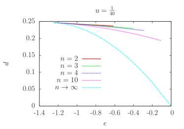
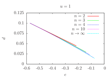
Figure 1: $e$ vs $d$ curves for $u=1/40$ and $u=1$ respectively, showing states occupying 1-strings and $n$-strings

By taking derivatives with respect to $u$, we can calculate the double occupancy $d$ as a function of $x$, and combining this with (26) we can study how $d$ changes with $e$ for the different families $n$. The results are shown in Fig. 1.

III.3 Double occupancy for thermal vs atypical states

It is interesting to compare the behaviour of the double occupancy in thermal states and the particular family of atypical states as identified above in Section III.2. We can calculate the energy density and double occupancy for typical states using the free energy of (20) as

$$\langle e\rangle_{\beta}=\frac{\partial}{\partial\beta}\big{(}\beta f\big{)},\qquad\langle d\rangle_{\beta}=\frac{\partial f}{\partial U}+\frac{1}{4},$$ (27)

where we have used the fact that we are working at half-filling. This determines $d$ as an implicit function of $e$ for thermal states. We note that this is of experimental relevance, as recent ultra-cold atomic experiments are able to directly measure the double occupancy in realisations of the one-dimensional Hubbard modelBloch .

In Fig. 2 we present results for the double occupancy as a function of the energy density for thermal states at several values of the interaction strength $u$. These are compared to the corresponding results for the finite entropy density atypical states with $n=4$ constructed in Section III.2.

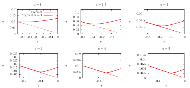
Figure 2: Double occupancy $d$ as a function of the energy density for thermal (solid lines) and atypical states (dashed lines).

We see that as the interaction strength $u$ is increased, the results for thermal and atypical states track one another for an increasing range of energy densities. On the other hand, for small values of $u$ the double occupancies of thermal and atypical states are very different at all energy densities.

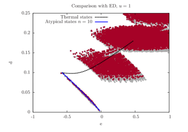
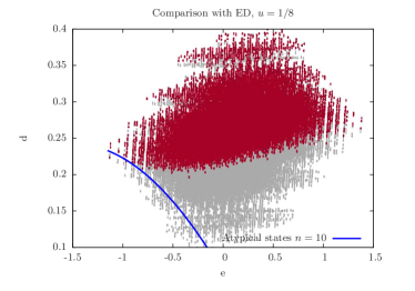
Figure 3: Comparison of thermal and typical states with exact diagonalisation data of Ref. hubb1, . Here the points indicate expectation values for eigenstates of the Hubbard model, where the spin singlets are highlighted in red.

These results can be used to shed some light on the role played by finite-size effects in the exact diagonalisation results of Ref. hubb1, . There the double occupancy was computed on lattices of up to $L=12$ sites and a very interesting change in behaviour of $e(d)$ was observed as a function of $u$. As shown in Fig. 3, for sufficiently large values of $u$ the there is a “band” of eigenstates in the $d-e$ plane that minimises $d$ at fixed $e$ and is separated from the region traced out by the other eigenstates. This is easily understood in terms of typical and atypical eigenstates. The special band of states is seen to track the $d(e)$ of our $n=4$ family of atypical states, while for most of the states $d(e)$ is centered around the result for typical states in the thermodynamic limit (as the system size in the numerical study is quite small we expect a significant spread around the thermodynamic limit result). At small values of $u$ the atypical states are no longer visible in $L=12$ numerical data, which are now all spread around the thermal thermodynamic limit result. This discrepancy has its origin in the strength of finite-size effects, which are more pronounced in the small-$u$ limit.

IV Particular atypical energy eigenstates: the “Heisenberg sector”

In Ref. hubb1, it was suggested that a particular class of eigenstates of the Hubbard Hamiltonian possess the QDL property. These states were identified for short chains by considering the strong coupling regime $t\ll U$. In this regime the spectrum breaks up into a sequence of narrow “bands” of states, which can be characterised by the expectation value of the double occupancy number operator. The states of interest constitute the lowest such band and are adiabatically connected to eigenstates without any doubly occupied sites in the limit $t/U\to 0$. As we are interested in the limit $L\to\infty$ at fixed $U$, our first task is to identify such states in terms of the Bethe Ansatz solution. This can be done either at the level of micro states in a (large) finite volume, or in terms of macro states in the thermodynamic limit QDLHubbard .

IV.1 Micro states

An important property of the exact solution of the Hubbard model is that it makes it possible to follow the evolution of particular eigenstates with the interaction parameter $u$. In the framework of the string hypothesisbook there is a one-to-one correspondence between energy eigenstates and solutions to the Bethe Ansatz equations (II), which, in turn, are uniquely characterised by sets of (half-odd) integers $I_{j}$, $J^{n}_{\alpha}$, $J{{}^{\prime}}^{n}_{\alpha}$. Fixing a particular set $\{I_{j},J^{n}_{\alpha},J{{}^{\prime}}^{n}_{\alpha}\}$ we may follow the corresponding solution of (II) as a function of $u$. This allows us to identify the special states considered in Ref. hubb1, as follows. In the limit $U\to\infty$ at fixed $L$ and half filling, the lowest energy states are obtained by setting

$$M^{\prime}=0\ ,$$ (28)

i.e. considering only states that do not contain any $k$-$\Lambda$ strings. This is because the latter contribute ${\cal O}(u)$ to the total energy, cf. (5). These states are characterised by the quantum numbers $J^{n}_{\alpha}$, which have ranges

$$|J^{n}_{\alpha}|\leq\frac{1}{2}\left(\frac{L}{2}-\sum_{m=1}^{\infty}t_{nm}M_{m}-1\right),\quad\alpha=1,\dots,M_{n}.$$ (29)

There is no freedom in choosing the $I_{j}$: they are given by

$$I_{j}=\begin{cases}-\frac{L}{2}+j&\text{if }\sum_{m}M_{m}\text{ is even}\\ -\frac{L+1}{2}+j&\text{if }\sum_{m}M_{m}\text{ is odd}\end{cases}\ ,\quad j=1,\dots L.$$ (30)

Importantly, the $I_{j}$ form a completely filled “Fermi sea”, just as they do in the ground state of the half-filled Hubbard model. It follows from the results of Ref. completeness, that the total number of such states is $2^{L}$. We call these states Heisenberg sector states.

IV.2 Macro states

At the level of macro states the Heisenberg sector corresponds to the requirement

$$\rho^{h}(k)=0={\sigma^{\prime}}_{n}^{p}(\Lambda)\ ,\ n=1,2,\dots$$ (31)

We note that the correspondence between (31) and the microscopic definition of IV.1 is to be understood in a thermodynamic fashion. There clearly will be eigenstates that are captured by (31), but go beyond the narrow specification we used in IV.1. For example, adding a finite number of $k$-$\Lambda$ strings will not change the macro state (31), as this affect the densities only to order ${\cal O}(L^{-1})$.

Importantly, the “freezing” of the charge degrees of freedom that characterises the Heisenberg sector implies that the thermodynamic entropy density for these macro states depends only on the spin degrees of freedom

$$s=\sum_{n=1}^{\infty}\int_{-\infty}^{\infty}d\Lambda\ {\cal S}\left[\sigma_{n}^{p}(\Lambda),\sigma_{n}^{h}(\Lambda)\right].$$ (32)

IV.2.1 Maximal entropy states in the Heisenberg sector

The next question we want to address is which macro states in the Heisenberg sector maximise the entropy at a given energy density. These states would be selected with probability $1$ if one randomly picked an eigenstate at a given energy density in an asymptotically large system. We start from the thermodynamic limit of the Takahashi equations (9) for Heisenberg sector states

$$\rho^{p}(k) = \frac{1}{2\pi}+\cos k\sum_{n=1}^{\infty}\int_{-\infty}^{\infty}d\Lambda\ {a_{n}(\Lambda-\sin k)}\sigma_{n}^{p}(\Lambda)\ ,$$

$$\sigma_{n}^{h}(\Lambda) = -\sum_{m=1}^{\infty}\int_{-\infty}^{\infty}d\Lambda^{\prime}A_{nm}(\Lambda-\Lambda^{\prime})\ \sigma_{m}^{p}(\Lambda^{\prime})+\int_{-\pi}^{\pi}dk\ {a_{n}(\sin k-\Lambda)}\ \rho^{p}(k)\ .$$ (33)

We then define an analogue of the free energy density by

$$f=e-{\cal T}s\ ,$$ (34)

where $e$ and $s$ are the energy and entropy densities of Heisenberg sector states and are given by (11) and (32) respectively. The “temperature” ${\cal T}$ is understood simply as a Lagrange parameter that allows us to fix the energy density. We now extremise the free energy with respect to the particle and hole densities, subject to (33). This fixes the ratios $\eta_{n}(\Lambda)=\frac{\sigma_{n}^{h}(\Lambda)}{\sigma^{p}_{n}(\Lambda)}$ to be solutions to the system of TBA-like equations

$$\ln\big{(}1+\eta_{n}(\Lambda)\big{)}=\frac{g_{1}(\Lambda)}{{\cal T}}+\sum_{m=1}^{\infty}\int_{-\infty}^{\infty}d\Lambda^{\prime}\ A_{nm}(\Lambda-\Lambda^{\prime})\ln\left[1+\frac{1}{\eta_{m}(\Lambda^{\prime})}\right],$$ (35)

where $g_{1}(\Lambda)=-4{\rm Re}\sqrt{1-(\Lambda-inu)^{2}}+4nu$. The entropy density for these macro states is given by

$$s=\sum_{n=1}^{\infty}\int_{-\infty}^{\infty}d\Lambda\left[\frac{g_{1}(\Lambda)}{{\cal T}}\sigma_{n}^{p}(\Lambda)+g_{2}(\Lambda)\ln\big{(}1+\eta_{n}^{-1}(\Lambda)\big{)}\right],$$ (36)

where $g_{2}(\Lambda)=\frac{1}{\pi}{\rm Re}\frac{1}{\sqrt{1-(\Lambda+inu)^{2}}}$.

V Entanglement entropy of Heisenberg sector states

As we have seen above, the Bethe Ansatz solution of the Hubbard model provides us with a means to compute the thermodynamic entropy density for any macro state. On the other hand, the notion of a QDL involves entanglement properties after a partial measurement. Implementing such partial measurements in the Bethe Ansatz framework is beyond the currently available methods. However, some information about entanglement properties of energy eigenstates can be inferred as follows. For short-ranged Hamiltonians there is a relation between the thermodynamic and entanglement entropies: if we consider a large subsystem $A$ of size $|A|$ in the thermodynamic limit, the volume term in the EE of an eigenstate $|\Psi\rangle$ is given by

$$S_{\rm vN,A}=s|A|+o(|A|),$$ (37)

where $s$ is the thermodynamic entropy density. As we have seen in (32), the thermodynamic entropy density of Heisenberg sector states depends only on the spin degrees of freedom. This then implies that the volume term in the EE is independent of the charge degrees of freedom, and depends on the spin sector only. In particular, as (37) is based only on the properties of the macro state under consideration, we know that microscopic rearrangements in the charge sector, such as introducing $k$-$\Lambda$ strings, will not affect (37). The emerging picture is consistent with expectations for a QDL state: the spin degrees of freedom exhibit a volume law EE, while the charge degrees of freedom are only weakly entangled. The spin degrees of freedom will be “heavy” in the terminology of Ref. qdl, at large values of $U$, because their bandwidth is proportional to $t^{2}/U$. The bandwidth of the charge degrees of freedom remains ${\cal O}(t)$ and they are therefore “light” in comparison. We stress that Heisenberg states obey (37) for any value of $u$, and the heavy vs light separation is not required. This is presumably a consequence of integrability.

Considerations based on the von Neumann EE fall short of the full QDL diagnostic proposed in Ref. qdl, , which requires carrying out a partial measurement of the spin degrees of freedom. Evidence based on a strong coupling analysis that supports the view that Heisenberg sector states pass the full QDL diagnostic has been put forward in Ref. QDLHubbard, .

VI Thermal states in the large-$U$ limit

We have constructed an exponential (in the system size) number of eigenstates, which exhibit QDL behaviour in the thermodynamic limit. However, these states are atypical in the sense introduced above: the most likely states at a given energy density are thermal. It is therefore instructive to contrast the entanglement properties of Heisenberg sector states with those of typical states. The latter are given as solutions of the systems (19) and (9) of coupled integral equations. While it is not possible to solve these analytically in general, in the limit of strong interactions analytic results can be obtained takahashiTBA2 ; Ha ; EEG . This is also the most interesting in the QDL context, as it provides a natural notion of light (charge) and heavy (spin) degrees of freedom. It is instructive to focus on the “spin-disordered regime”

$$\frac{4t^{2}}{U}\ll T\ll U\ .$$ (38)

This corresponds to temperatures that are small compared to the Mott gap, but large compared to the exchange energy. This is a natural regime in which one may expect the proposed physics to be realised. Here one hasEEG

$$\rho^{h}(k)={\cal O}\big{(}e^{-u/T}\big{)}\ ,\quad{\sigma^{\prime}}^{p,h}_{n}(\Lambda)={\cal O}\big{(}e^{-u/T}\big{)}.$$ (39)

Substituting this into the general expression (11) for the thermodynamic entropy density we obtain

$$s=\sum_{n=1}^{\infty}\int_{-\infty}^{\infty}d\Lambda\ {\cal S}\left[{\sigma_{n}}^{p}(\Lambda),{\sigma_{n}}^{h}(\Lambda)\right]+{\cal O}\Big{(}\frac{u}{T}e^{-u/T}\Big{)}.$$ (40)

Finally, using the relation between thermodynamic and EE (37) we conclude that for thermal states in the spin-disordered regime the contribution of the charge degrees of freedom contribute to the volume term is

$$S_{\rm vN,A} = \big{(}s_{\rm spin}+s_{\rm charge}\big{)}|A|+o\big{(}|A|\big{)}\ ,$$

$$s_{\rm spin} = {\cal O}(1)\ ,\quad s_{\rm charge}={\cal O}\Big{(}\frac{u}{T}e^{-u/T}\Big{)}\ .$$ (41)

Here $s_{\rm charge}$ includes the contributions from pure charge degrees of freedom as well as bound states of spin and charge. Importantly, unlike Heisenberg sector states, typical states have a contribution from the charge degrees of freedom to the volume term. However, this contribution is exponentially small in $u/T$ and therefore only visible for extremely large subsystems. While we have focused on the spin-disordered regime, the behaviour (41) extends to thermal states for all $0<T\ll U$. In Ref. QDLHubbard, , behaviour of the kind (41) (for the entanglement entropy after a partial measurement) was proposed as a “weak” form of a QDL, which one may expect to occur quite generically in strong coupling limits.

VII Conclusions

We have presented evidence that the QDL state of matter is realised in the strong sense proposed in Ref. qdl, for a particular class of eigenstates of the one-dimensional half-filled Hubbard model. We have defined the states constituting this class in the framework of the Bethe Ansatz by freezing the charge degrees of freedom in the configuration corresponding to the half-filled ground state. For such states, we have explicity shown that the charge degrees of freedom (“light particles”) do not contribute to the volume term of the bipartite EE.

The Heisenberg sector states are unusual in a precise sense: the EE for typical (thermal) states at a finite energy density has a volume-law contribution that involves the charge degrees of freedom even for large $U/t$. We have shown that in a particular regime at strong coupling the contribution is of the form (41), i.e.

$$S_{\rm vN,A} =\big{(}s_{\rm spin}+s_{\rm charge}\big{)}|A|+o\big{(}|A|\big{)},$$ (42)

$$s_{\rm spin} ={\cal O}(1)\ ,\quad s_{\rm charge}={\cal O}\Big{(}\frac{u}{T}e^{-u/T}\Big{)}\ ,\quad$$

and we have argued that for $U\gg t$ this form is obtained quite generally at energy densities that are small compared to $U$. We expect a similar volume law to occur in the EE after a measurement of all spins. This suggests the notion of a “weak” variant of a QDL, which is characterised a volume term in the EE after measurement of the heavy degrees of freedom that is parametrically small, and practically unobservable except in extremely large systems. We expect that this weak scenario is not tied to integrability, and should be realised quite generally in strong coupling regimes. This is supported by the strong-coupling expansion results of Ref. QDLHubbard, , which do not rely on integrability.

Given that Heisenberg sector states are atypical and hence rare, a natural question is how they can be accessed in practice. In principle this can be achieved by means of a quantum quench EFreview from a suitably chosen initial state. As the Hubbard model is integrable the expectation values of its infinite number of conservation laws are fixed by the initial state. At late times after the quench the system relaxes locally to an atypical state that is characterised by these expectation values. This provides a general mechanism for realising atypical states. In order to access a Heisenberg sector state the initial conditions need to be fine tuned. It would be interesting to investigate what class of initial states will give rise to Heisenberg sector steady states. Realising the weak variant (41) of a QDL is a much simpler matter. Fixing the energy density to be small compared to the Mott gap is sufficient to obtain a non-equilibrium steady state that realises the weak form of a QDL. In the Hubbard model this corresponds to the spin-incoherent Mott insulating regime. Dynamical properties in this regime can be analyzed by numerical as well as strong-coupling methodsspinincoherent .

- (1) J. von Neumann, Zeit. Phys. 57, 30 (1929); translation European Phys. J. H 35, 201 (2010).
- (2) M. Greiner, O. Mandel, T.W. Hänsch and I. Bloch, Nature 419, 51-54 (2002).
- (3) T. Kinoshita, T. Wenger and D. S. Weiss, Nature 440, 900 (2006).
- (4) S. Hofferberth, I. Lesanovsky, B. Fischer, T. Schumm and J. Schmiedmayer, Nature 449, 324-327 (2007).
- (5) L. Hackermuller, U. Schneider, M. Moreno-Cardoner, T. Kitagawa, S. Will, T. Best, E. Demler, E. Altman, I. Bloch and B. Paredes, Science 327, 1621 (2010).
- (6) S. Trotzky Y.-A. Chen, A. Flesch, I. P. McCulloch, U. Schollwöck, J. Eisert and I. Bloch, Nature Phys. 8, 325 (2012).
- (7) M. Gring, M. Kuhnert, T. Langen, T. Kitagawa, B. Rauer, M. Schreitl, I. Mazets, D. A. Smith, E. Demler and J. Schmiedmayer, Science 337, 1318 (2012).
- (8) M. Cheneau, P. Barmettler, D. Poletti, M. Endres, P. Schauss, T. Fukuhara, C. Gross, I. Bloch, C. Kollath and S. Kuhr, Nature 481, 484 (2012).
- (9) T. Langen, R. Geiger, M. Kuhnert, B. Rauer, and J. Schmiedmayer, Nature Physics 9, 640 (2013).
- (10) F. Meinert, M.J. Mark, E. Kirilov, K. Lauber, P. Weinmann, A.J. Daley, and H.-C. Nägerl, Phys. Rev. Lett. 111, 053003 (2013).
- (11) N. Navon, A.L. Gaunt, R.P. Smith and Z. Hadzibabic, Science 347, 167 (2015).
- (12) M. Schreiber, S.S. Hodgman, P. Bordia, H.P. Lüschen, M.H. Fischer, R. Vosk, E. Altman, U. Schneider and I. Bloch, Science 349, 842 (2015).
- (13) J. M. Deutsch, Phys. Rev. A 43, 2046 (1991).
- (14) M. Srednicki, Phys. Rev. E 50, 888 (1994).
- (15) M. Srednicki, J. Phys. A 32, 1163 (1998).
- (16) L. D’Alessio, Y. Kafri, A. Polkovnikov and M. Rigol, Adv. Phys. 65, 239 (2016).
- (17) M. Rigol, V. Dunjko, V. Yurovsky and M. Olshanii, Phys. Rev. Lett. 98, 50405 (2007).
- (18) P. Calabrese and J. Cardy, J. Stat. Mech. P06008, (2007).
- (19) F. H. L. Essler and M. Fagotti J. Stat. Mech. 064002 (2016).
- (20) M. A. Cazalilla and M.-C. Chung, J. Stat. Mech. 064004 (2016).
- (21) L. Vidmar and M. Rigol, J. Stat. Mech. 064007 (2016).
- (22) E. Ilievski, J. De Nardis, B. Wouters, J.-S. Caux, F.H.L. Essler and T. Prosen, Phys. Rev. Lett. 115, 157201 (2015).
- (23) A. C. Cassidy, C. W. Clark, M. Rigol, Phys. Rev. Lett 106, 140405 (2011).
- (24) J.S. Caux and F.H.L. Essler, Phys. Rev. Lett. 110, 257203 (2013).
- (25) I. V. Gornyi, A. D. Mirlin and D. G. Polyakov, Phys. Rev. Lett. 95, 206603 (2005).
- (26) D. M. Basko, I. L. Aleiner and B. L. Altshuler, Annals of Physics 321, 1126 (2006).
- (27) V. Oganesyan and D. A. Huse, Phys. Rev. B75, 155111 (2007).
- (28) A. Pal and D. A. Huse, Phys. Rev. B82, 174411 (2010).
- (29) B. Bauer and C. Nayak, J. Stat. Mech. 09005 (2013).
- (30) J. Z. Imbrie, J. Stat. Phys. 163, 998 (2016).
- (31) M. Serbyn, Z. Papi´c, and D. A. Abanin, Phys. Rev. Lett. 111, 127201 (2013).
- (32) D. A. Huse, R. Nandkishore, and V. Oganesyan, Phys. Rev. B90, 174202 (2014).
- (33) T. Grover and M. P. A. Fisher, J. Stat. Mech. P10010 (2014).
- (34) J.R. Garrison, R.V. Mishmash and M.P.A. Fisher, Phys. Rev. B95, 054204 (2017).
- (35) T. Veness, F. H. L. Essler, M. P. A. Fisher, arXiv:1611.02075.
- (36) F. H. L. Essler, H. Frahm, F. Göhmann, A. Klümper, and V. E. Korepin, The One-Dimensional Hubbard Model, Cambridge University Press, Cambridge (2005).
- (37) V. Alba, M. Fagotti and P. Calabrese, J. Stat. Mech., P10020 (2009).
- (38) M. Takahashi, Prog. Theor. Phys. 47, 69 (1972).
- (39) F.H.L. Essler, V.E. Korepin and K. Schoutens, Phys. Rev. Lett. 67, 3848 (1991).
- (40) F.H.L. Essler, V.E. Korepin, and K. Schoutens, Nucl. Phys. B372, 559 (1992).
- (41) T. A. Hilker, G. Salomon, F. Grusdt, A. Omran, M. Boll, E. Demler, I. Bloch, C. Gross, arXiv:1702.00642.
- (42) F.H.L. Essler, V.E. Korepin, and K. Schoutens, Nucl. Phys. B384, 431 (1992).
- (43) M. Takahashi, Prog. Theor. Phys. 52, 103 (1974).
- (44) Z.N.C. Ha, Phys. Rev. B46, 12205 (1992).
- (45) S. Ejima, F.H.L. Essler and F. Gebhard, J. Phys. A39, 4845 (2006).
- (46) A. Nocera, F.H.L. Essler and A.E. Feiguin, in preparation.