Global Properties of M31’s Stellar Halo from the SPLASH Survey: III. Measuring the Stellar Velocity Dispersion Profile

Abstract

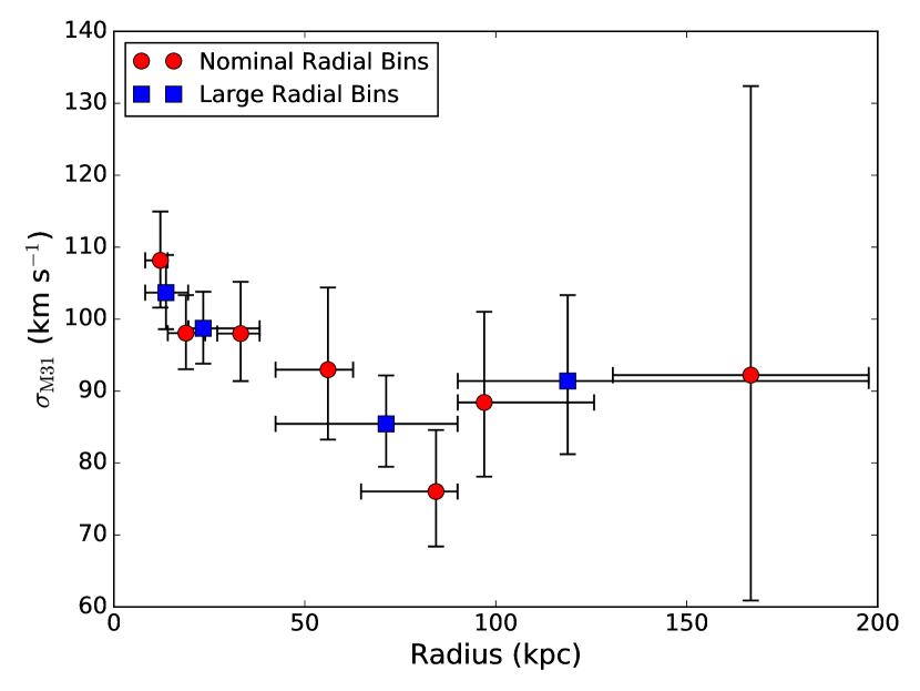
We present the velocity dispersion of red giant branch (RGB) stars in M31’s halo, derived by modeling the line of sight velocity distribution of over 5000 stars in 50 fields spread throughout M31’s stellar halo. The dataset was obtained as part of the SPLASH (Spectroscopic and Photometric Landscape of Andromeda’s Stellar Halo) Survey, and covers projected radii of 9 to 175 kpc from M31’s center. All major structural components along the line of sight in both the Milky Way (MW) and M31 are incorporated in a Gaussian Mixture Model, including all previously identified M31 tidal debris features in the observed fields. The probability an individual star is a constituent of M31 or the MW, based on a set of empirical photometric and spectroscopic diagnostics, is included as a prior probability in the mixture model. The velocity dispersion of stars in M31’s halo is found to decrease only mildly with projected radius, from 108  km s^-1 in the innermost radial bin (8.2 to 14.1 kpc) to $\sim 80$ to 90  km s^-1 at projected radii of $\sim 40$ – 130 kpc, and can be parameterized with a power-law of slope $-0.12\pm 0.05$. The quoted uncertainty on the power-law slope reflects only the precision of the method, although other sources of uncertainty we consider contribute negligibly to the overall error budget.

1 Introduction

The orbits of satellite dwarf galaxies, globular clusters, and halo stars trace the mass distribution of their host system to large radii and can be used to estimate the total mass of the host system. The three-dimensional space motions of these tracers is currently out of reach for all but the Milky Way (MW) and its closest satellite galaxies. Thus, in more distant systems the line of sight velocity distribution of these tracers is the key observable and can be used to estimate the enclosed mass via estimators of varying complexity (e.g., Cappellari et al., 2006; Watkins et al., 2010; Wolf et al., 2010; Gnedin et al., 2010; Amorisco & Evans, 2012).

The proximity of the Andromeda galaxy (M31) allows measurement of the line of sight velocity distributions of all three of these tracers. Estimates of M31’s mass have previously been made based on the velocity distributions of M31’s dwarf satellite galaxies (Watkins et al., 2010; Tollerud et al., 2012) and globular clusters (Veljanoski et al., 2014). The mass estimate based on M31’s dwarf satellites is sensitive to which satellites are included in the measurement: satellites that are not on virialized orbits (i.e., that are on their first infall or are not gravitationally bound) can significantly skew the mass estimate. Meanwhile, the globular cluster population shows significant rotation (Veljanoski et al., 2013), which must be modeled, and also has a significant fraction of clusters that are statistically likely to be associated with halo substructure (Mackey et al., 2010; Veljanoski et al., 2014).

M31’s halo stars provide a dense network of mass tracers that can provide an independent mass estimate. The density of halo stars allows the kinematics of distinct tidal debris features to be accounted for directly in the modeling of the velocity distribution of the underlying halo population. A mass estimate based on the velocity distribution of halo stars can thus provide an important comparison to mass estimates from the satellite or globular cluster system. Currently, M31 is the only external galaxy for which we can compare the velocity distributions of all three tracer systems to large radii. This will provide an important calibration for interpreting mass estimates in more distant galaxies that are based on the galaxy’s globular cluster or dwarf satellite system.

The kinematics of M31 halo stars, especially when combined with chemical abundance measurements, can also be used to investigate the the inner regions of M31’s stellar halo. In the inner regions, we expect to find a mix of in situ and accreted halo stars based on theoretical grounds (e.g., Abadi et al., 2006; Zolotov et al., 2009; Purcell et al., 2010; Cooper et al., 2010; Font et al., 2011). Observations of the inner regions of the MW have recently ignited a vigorous debate regarding the evidence for multiple halo populations (e.g., Majewski, 1992; Carollo et al., 2010; Schönrich et al., 2011; Beers et al., 2012; Schönrich et al., 2014). M31 provides the only external galaxy for which we can currently place observational constraints on the presence of multiple formation avenues for the stellar halo.

Large spectroscopic surveys in M31 have provided line of sight velocity measurements for tens of thousands of stars in M31. The majority of the analysis of the velocity measurements has been focused on characterizing substructure (Ibata et al., 2004; Guhathakurta et al., 2006; Kalirai et al., 2006a; Gilbert et al., 2007; Chapman et al., 2008; Gilbert et al., 2009b; Fardal et al., 2012; Mackey et al., 2014; Kafle et al., 2017), measuring the internal velocity dispersion of M31 satellite galaxies (Chapman et al., 2005; Geha et al., 2006; Letarte et al., 2009; Kalirai et al., 2009, 2010; Geha et al., 2010; Collins et al., 2010, 2011a; Ho et al., 2012; Tollerud et al., 2012, 2013; Howley et al., 2013; Collins et al., 2013, 2014; Martin et al., 2014), and measuring the dynamics of the disk (Ibata et al., 2005; Collins et al., 2011b; Dorman et al., 2013, 2015).

Existing measurements of the velocity dispersion of M31’s stellar halo have been limited to the inner regions of the halo and have primarily been made in spectroscopic fields that are dominated by M31 disk stars. Chapman et al. (2006) used spectra obtained in fields throughout M31’s disk, at projected radii of 9 to 70 kpc, to measure the velocity dispersion of M31’s halo as a function of projected radius. To avoid contamination from M31’s disk, substructure in M31, and MW stars, Chapman et al. employed window functions in velocity and a constrained maximum-likelihood analysis, fixing the mean velocity of M31’s stellar halo and iteratively rejecting spectroscopic fields. The measured gradient in the velocity dispersion was strongly dominated by spectroscopic fields within 40 kpc of M31’s center, and implies a central velocity dispersion of 152  km s^-1, decreasing at a rate of $-0.9$  km s^-1 kpc^-1. Gilbert et al. (2007) modeled the velocity distribution of spectroscopically confirmed M31 stars along the minor axis from 9 to 30 kpc, performing a maximum-likelihood analysis assuming both an M31 halo and substructure component. Gilbert et al. measured a velocity dispersion of 129  km s^-1 for the halo over this radial range. Most recently, Dorman et al. (2012) analyzed spectra in large contiguous regions in M31’s inner disk ($R\lesssim 20$ kpc). Dorman et al. performed a Markov chain Monte Carlo (MCMC) analysis of spectroscopically confirmed M31 red giant branch stars, simultaneously fitting for the disk, substructure, and halo components. Dorman et al. detected significant spheroid rotation in the inner regions, and found a decrease in the line of sight velocity dispersion of M31’s halo, from $\sim 140$  km s^-1 at 7 kpc to $120$  km s^-1at 14 kpc on the major axis. In their regions of radial overlap, the existing measurements are consistent with one another at the $\lesssim 2\sigma$ level.

The SPLASH (Spectroscopic and Photometric Landscape of Andromeda’s Stellar Halo; Guhathakurta et al., 2005; Gilbert et al., 2006) survey has amassed an archive of tens of thousands of spectra in lines of sight throughout M31’s halo, disk, and dwarf galaxies (e.g., Kalirai et al., 2010; Tollerud et al., 2012; Gilbert et al., 2012, 2014; Dorman et al., 2012, 2015). A large portion of the SPLASH spectroscopic fields are in the outer halo of M31, far removed from M31’s disk. In the first two papers of this series, we used counts of spectroscopically confirmed M31 RGB stars in 38 fields to measure an $\sim r^{-2}$ surface brightness profile for M31’s stellar halo out to 175 kpc (Gilbert et al., 2012) and confirmed the existence of a large scale metallicity gradient in M31’s halo from 10 to 100 kpc (Gilbert et al., 2014).

In this contribution, we model the line-of-sight velocity distributions of more than 5000 stars in 50 fields spread throughout M31’s stellar halo, with projected radii from M31’s center of 9 to 175 kpc. None of the fields are located on M31’s disk. We do not employ any windowing functions on the line of sight velocity, nor do we make any cuts to the spectroscopic sample based on likely membership in the M31 or MW populations, as has been done in previous work. Rather, we employ MCMC methods to sample the posterior distribution functions for the full set of model parameters needed to describe the kinematical components that have been previously identified within the SPLASH survey.

This paper is organized as follows. Section 2 provides a brief overview of the spectroscopic dataset. Section 3 describes the multiple stellar populations present in the spectroscopic fields and the empirical diagnostics available for assigning probabilities of membership. It also explains the motivation underlying our choice to include all observed MW and M31 halo stars in our fitting of the velocity distribution. Section 4 describes the MCMC analysis, including the formulation of the likelihood function and the choice of priors. Section 5 describes the results of the MCMC analysis of the line-of-sight velocity distributions for the primary model parameters of interest, including the parameterization of the velocity dispersion of M31’s stellar halo with radius (Section 5.1). Appendices present marginalized one- and two-dimensional posterior probability distributions for all model parameters, including those not discussed in Section 5.

All radii from M31’s center refer to the projected distance in the sky tangent plane. For consistency with previous papers in this series, and to allow direct comparisons with other results, a distance modulus of 24.47^m is assumed for conversions of angular to physical units, which corresponds to a distance to M31 of 783 kpc (Stanek & Garnavich, 1998; McConnachie et al., 2005). However, we note that this distance is slightly greater than the recent, smaller distance modulus estimate of 24.38^m based on measurements of Cepheid variables (Riess et al., 2012). Where relevant, we adopt the Planck Collaboration 2015 cosmology (Planck Collaboration et al., 2016).

2 The SPLASH Data Set

The majority of the SPLASH data ($\sim 90$% of the spectroscopic masks) have been presented in earlier contributions. The new spectroscopic data have been obtained with an identical observational setup and reduced using the same data reduction pipelines. The spectroscopic masks were designed using imaging data that were obtained and reduced in the same imaging campaigns as the fields used to design earlier spectroscopic masks. Thus, we only briefly summarize the spectroscopic data and its reduction below. Readers are referred to Gilbert et al. (2012, 2014) for details of the photometric and spectroscopic data reduction.

2.1 Field Locations

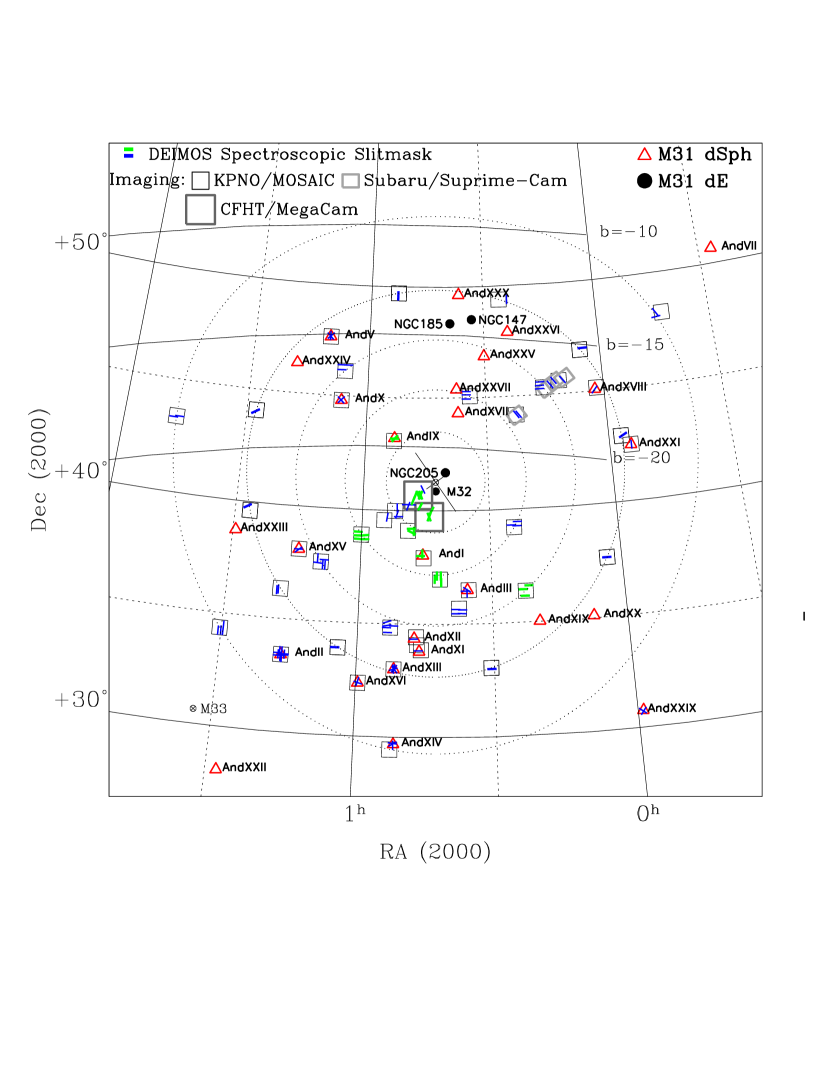
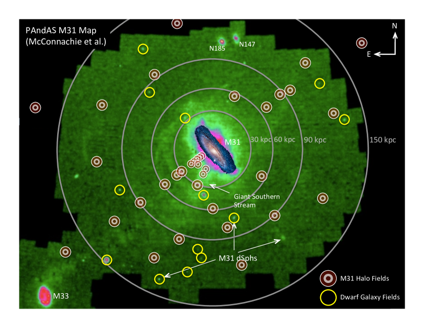
The stellar spectra were obtained with 124 multi-object spectroscopic slitmasks in 50 fields spread throughout M31’s stellar halo (Figure 1). The masks span a large range in azimuth and projected radii from the center of M31. The fields were chosen to target relatively smooth areas of M31’s halo, individual tidal debris features, and dwarf satellites (Figure 2).

Figure 1: Locations of the spectroscopic fields. The location and orientation of each spectroscopic mask is denoted with a small rectangle; green rectangles denote spectroscopic masks with kinematically identified substructure. Larger rectangles denote the location and extent of the KPNO/Mosaic (black), CFHT/MegaCam (dark grey) and Subaru/Suprime-Cam (light grey) images used to design the masks. The location of the dwarf elliptical (black circles) and dwarf spheroidal (open triangles) satellites of M31 are also shown. M31’s center is marked by an open circle, and the orientations of M31’s major and minor axes are illustrated with the long and short solid lines. The dotted circles have radii of 2, 4, 6, 8 and 11 degrees from M31’s center.

Figure 2: Approximate locations of the spectroscopic fields overlaid on the PAndAS starcount map (McConnachie et al., 2009). Spectroscopic fields designed primarily to target M31’s dwarf galaxies are denoted by open yellow circles. The remaining fields target M31’s halo, and include fields on several large tidal debris features. Two dwarf spheroidal fields, And XIV and And XXIX, are not shown; they are to the south of M31, beyond the bounds of the figure.

2.2 Target Selection

The majority of the multi-object spectroscopic slitmasks were designed from images in the Washington system $M$ and $T_{2}$ filters and the intermediate-width DDO51 filter, obtained with the Mosaic camera on the 4-m Mayall telescope at Kitt Peak National Observatory (KPNO). (Ostheimer, 2003; Beaton, 2014). The innermost spectroscopic slitmasks were designed using $g^{\prime}$ and $i^{\prime}$ band imaging obtained with MegaCam instrument on the 3.6-m Canada-France-Hawaii Telescope (CFHT) (Kalirai et al., 2006a). A small number of spectroscopic masks in the outer halo of M31 were designed from Johnson-Cousins $V$ and $I$ band imaging obtained with the Suprime-Cam instrument on the Subaru Telescope (fields ‘streamE’ and ‘streamF’; Tanaka et al., 2010) and the William Herschel Telescope (field ‘and10’; Zucker et al., 2007).

Stars were prioritized for inclusion on the spectroscopic masks based on their colors and magnitudes. Stars with colors and magnitudes consistent with RGB stars at the distance of M31 were assigned high priority for inclusion on the spectroscopic masks, with brighter RGB stars (within $\sim 1$ to 1.5 magnitudes of the tip of the red giant branch) given highest priority. When available, the surface-gravity sensitive intermediate-band DDO51 photometry was also used to prioritize stars with a high probability of being RGB stars (based on their location in the $M-T_{2}$, $M-$DDO51 color-color diagram; Majewski et al., 2000).

2.3 Spectroscopic Observations

The spectra were obtained with the DEIMOS spectrograph on the Keck II 10-m telescope over ten observing seasons (Fall 2002 – 2011). All of the spectra were obtained using the 1200 line mm^-1 grating, which produces a dispersion of $\rm 0.33~{}\AA$ pix^-1. The survey used a slit width of 1”, which yields a resolution of 1.6Å FWHM. The wavelength range of the observed spectra is $\lambda\lambda\sim$ 6450 – 9150Å, which includes the Ca ii triplet absorption feature ($\sim 8500$Å) and the Na i absorption feature (8190Å). The Keck/DEIMOS spectra were reduced using the spec2d (flat-fielding, night-sky emission line removal, and extraction of one-dimensional spectra) and spec1d (redshift measurement) software developed at the University of California, Berkeley (Cooper et al., 2012; Newman et al., 2013).

Only stellar spectra with secure velocity measurements are included in the final data set (Gilbert et al., 2006). A heliocentric correction is applied to the measured line of sight velocities as well as a correction for imperfect centering of the star within the slit (using the observed position of the atmospheric $A$-band absorption feature relative to night sky emission lines; Simon & Geha, 2007; Sohn et al., 2007).

The mean (median) S/N per Angstrom of the stellar spectra with secure velocity measurements is 11.7 (8.2). The mean (median) S/N per Angstrom of the spectra of stars that are more probable to be M31 stars than MW stars (Section 3.2) is 7.8 (4.4). The mean (median) velocity measurement uncertainty of all stellar spectra with secure velocity measurements is 5.7  km s^-1 (4.8  km s^-1), while the mean (median) velocity uncertainty of stars more probable to be M31 stars than MW stars is 6.5  km s^-1 (5.6  km s^-1). The uncertainties on the velocity measurements are calculated by adding in quadrature the random velocity measurement uncertainty, estimated from the cross-correlation routine, and a systematic uncertainty of 2.2  km s^-1, estimated from repeat observations of stars (Simon & Geha, 2007).

3 Separation of Stellar Populations

The final dataset of over 6600 stellar spectra is drawn from multiple stellar populations in M31 and along the line of sight to M31, including distinct tidal debris features within M31’s halo, dwarf satellites of M31, the Milky Way disk and halo, and finally the relatively smooth, underlying M31 halo whose velocity distribution we aim to measure. These populations all have some amount of overlap in line-of-sight velocity space. However, the photometry and stellar spectra provide additional discriminating power beyond the line of sight velocities for separating these populations. We briefly describe below the methods used to assign membership, or probabilities of membership, among the various populations. Each of these methods have been utilized in earlier publications, to which readers are referred for greater detail.

3.1 Removal of Dwarf Galaxy Members

Almost one-third of the fields that are farther than 4^∘ from M31’s center targeted dwarf satellite galaxies (Figure 1; Majewski et al., 2007; Kalirai et al., 2009, 2010; Tollerud et al., 2012). In these fields, a significant number of the stars observed on each spectroscopic mask are dSph members, rather than M31 halo stars or MW stars along the line of sight.

Stars that are likely to be gravitationally bound to a dwarf satellite galaxy are identified following the method outlined by Gilbert et al. (2009b). M31’s dSphs are spatially compact, have small velocity dispersions, and span a limited range of [Fe/H]. The spatial extents of the majority of the M31 dSphs are small enough that they cover only a portion of a DEIMOS spectroscopic slitmask. Only stars within the King limiting radius are considered potential dSph members. Stars that are outside the King limiting radius are included in our final dataset. Thus we explicitly classify any extra-tidal dSph stars as M31 halo stars. This number is small: only $\sim 5$% of the stars beyond the King limiting radius in dSph fields have velocities and $\rm[Fe/H]$ values consistent with the dSph. In addition, any stars within the King limiting radius of the dSph but well removed from the distribution of dSph stars in line of sight velocity or $\rm[Fe/H]$ are classified as M31 halo stars. The interested reader can find examples for And I and And III in Figures 3 and 4 of Gilbert et al. (2009b).

After removing stars classified as dSph members, the final dataset contains 5299 stars.

3.2 Likelihood of M31 or MW Membership

We use the method established by Gilbert et al. (2006) to determine the likelihood that an individual star is a red giant branch star in M31 or a foreground MW dwarf star along the line of sight to M31. The Gilbert et al. method determines the probability a star is an M31 red giant branch or MW dwarf star from multiple photometric- and spectroscopic-based diagnostics. The full set of diagnostics includes (1) line-of-sight velocity, (2) location in the ($M-T_{2}$, $M-$DDO51) color-color diagram (when available), (3) strength of the Na i doublet absorption line as a function of ($V-I$) color, (4) location in the ($I$, $V-I$) color-magnitude diagram, and (5) comparison of spectroscopic and photometric metallicity estimates. Each diagnostic provides a (log-)likelihood that the star is an RGB or dwarf star: $L={\rm log}_{10}(P_{\rm RGB}/P_{\rm dwarf}$). The overall likelihood, $\langle L_{i}\rangle$, that a star is an M31 red giant or MW dwarf is defined as the sum of the individual log-likelihoods for each diagnostic (i.e., the product of the likelihoods).

An additional factor not included in the Gilbert et al. method is projected radius from M31’s center: the relative stellar density of M31 and MW populations changes dramatically as a function of M31-centric radius. For a given set of values of the stellar properties included in $\langle L_{i}\rangle$, a star is in fact more likely to be an M31 star in the inner regions compared to the outer regions. This is described in more detail in Section 4.2.3, where we explicitly include this in the model.

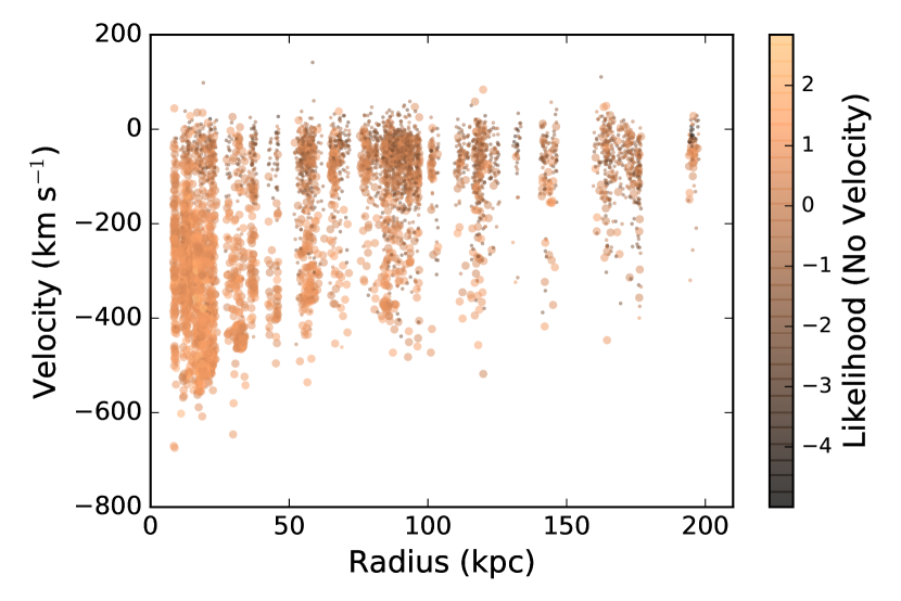
Since our aim is to model the stellar velocities, we do not include the velocity diagnostic in the computation of $\langle L_{i}\rangle$. Figure 3 shows the velocity of stars as a function of projected radius from M31, color-coded by $\langle L_{i}\rangle$ values computed with (left) and without (right) the velocity diagnostic. When velocity is included in the $\langle L_{i}\rangle$ computation, there is a strong trend of increasing $\langle L_{i}\rangle$ with decreasing line-of-sight velocity, which is a direct result of using the velocity diagnostic in the $\langle L_{i}\rangle$ calculation. Although weaker, a correlation of $\langle L_{i}\rangle$ with line of sight velocity is still evident when velocity is not included in the $\langle L_{i}\rangle$ computation, reflecting the velocity distributions of the M31 and MW populations.

Figure 3: Line of sight, heliocentric velocity of every star in the sample as a function of projected radius, color-coded by the likelihood of MW or M31 membership, $\langle L_{i}\rangle$, including (left) and excluding (right) the velocity diagnostic. Stars classified by their $\langle L_{i}\rangle$ values as as M31 stars ($\langle L_{i}\rangle$$>0$) are shown as large points, while stars classified as MW stars are shown as small points ($\langle L_{i}\rangle$$\leq 0$ or very blue stars; Section 3.2). M31’s systemic line of sight velocity is $\sim-300$  km s^-1. While including velocity in the $\langle L_{i}\rangle$ calculation results in a cleaner sample of M31 stars, it also introduces a strong bias in the velocity distribution of any sample selected based on an $\langle L_{i}\rangle$ threshold.

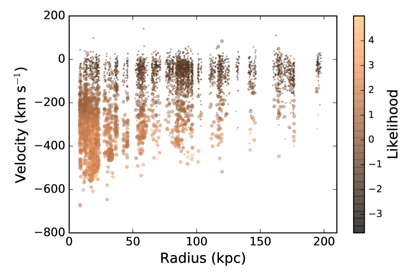
In previous papers, we defined samples of M31 and MW stars based on $\langle L_{i}\rangle$ thresholds, and stars significantly bluer than the most metal-poor, 10 Gyr RGB isochrone have been classified as securely identified MW stars regardless of their $\langle L_{i}\rangle$ values (Gilbert et al., 2006). This acknowledged that many of the empirical diagnostics have little discriminating power for stars with blue colors, as well as the fact that these stars are much more likely to be MW stars than RGB stars in M31. In this paper we use the $\langle L_{i}\rangle$ values directly, rather than using subsets of stars classified as belonging to MW or M31. Thus we must choose how to treat stars bluer than the most metal-poor RGB isochrone in the following analysis. Rather than removing them from the sample altogether, we set their $\langle L_{i}\rangle$ values to $-5$. This places these blue stars in the tail of the $\langle L_{i}\rangle$ distribution of MW stars, acknowledging that it is very unlikely for them to be M31 RGB stars. This is equivalent to what has been done in our previous papers. The sensitivity of the final results to this choice is explored in Section 5.2.

3.3 Probability of Belonging to Tidal Debris Features

Kinematically cold tidal debris features have been identified in a significant fraction of the spectroscopic masks (Figures 1 and 2). Many of the tidal debris features identified in individual fields are related to a single accretion event: the Giant Southern Stream and its associated shell features (e.g., Ibata et al., 2001; Fardal et al., 2007; Gilbert et al., 2007, 2009b).

Each of the tidal debris features in the dataset have been identified and characterized via maximum-likelihood, multi-Gaussian fits to the velocity distribution of M31 stars in the field, and presented in previous papers (Guhathakurta et al., 2006; Kalirai et al., 2006a; Gilbert et al., 2007, 2009b, 2012). Details of the fitting technique can be found in the papers by Gilbert et al. (2007, 2012). Each maximum-likelihood fit includes a Gaussian with a large velocity dispersion, representing the underlying, kinematically hot stellar halo, and additional Gaussian components with small velocity dispersions, representing the kinematically cold stellar streams.

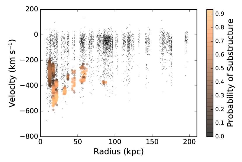
The velocity distribution of the M31 halo was held fixed in all the published fits, with a mean heliocentric velocity of $\langle v_{\rm hel}\rangle=-300$  km s^-1 (M31’s systemic velocity) and velocity dispersion of $\sigma_{\rm v}=129$  km s^-1 (Gilbert et al., 2007). The maximum-likelihood fits provide an estimate of the mean velocity, velocity dispersion, and fraction of M31 halo stars in each of the kinematically cold tidal debris features in a field. Using the maximum-likelihood fits, the probability that any individual M31 star belongs to the kinematically hot halo or a kinematically cold tidal debris feature can be computed. Figure 4 shows the line of sight velocity as a function of projected radius of all M31 and MW stars in the dataset, color-coded by the probability the star belongs to tidal debris.

Figure 4: Line of sight, heliocentric velocity of every star in the sample as a function of projected radius, color-coded by the probability the star belongs to substructure. The probabilities were computed using previously published maximum-likelihood fits to the velocity distribution of M31 stars (Section 3.3). Stars with a probability greater than 0.2 of belonging to substructure are shown as large points. The majority of identified tidal debris features in our dataset have velocities more negative than M31’s systemic velocity ($v_{\rm sys}=-300$  km s^-1).

3.4 Challenges of Selecting an M31 Halo Sample

In previous studies, we successfully identified M31 and MW samples using cuts on the various membership criteria. This work has included analyses of substructure (Gilbert et al., 2007, 2009b, 2009a), the surface brightness profile of M31’s halo (Gilbert et al., 2012), and the metallicity profile of M31’s halo (Kalirai et al., 2006b; Gilbert et al., 2014). Depending on the analysis, the sample selection was tuned to favor either a complete sample with some amount of contamination, or a clean but incomplete sample with minimal contamination. To produce the cleanest sample of M31 stars, many of the analyses required that a star be 3 times as likely to be an M31 red giant than a foreground MW dwarf star to be included in the M31 sample (Section 3.2).

However, simple threshold cuts on membership criteria are insufficient for the current analysis of the M31 halo velocity distribution, with the exception of stars belonging to the dwarf satellites of M31. We maintain the simple cut described above (Section 3.1) to identify and remove dSph stars from the sample. The small velocity dispersions, limited range of color (due to the limited range in [Fe/H] of the dSph stars) and relatively well defined spatial boundaries of the M31 dSphs allow us to identify and remove probable dwarf satellite members while minimally affecting the observed velocity distribution of M31 halo and MW stars in those fields. Even in dSph fields with relatively high densities of halo stars, at most two or three M31 halo stars are removed from the sample. Moreover, the dSphs in the sample have a broad range of systemic line of sight velocities. Thus, the small amount of incompleteness introduced into the M31 and MW dataset by removing dSph stars will not introduce a bias in the resulting velocity distribution.

In contrast, stars belonging to tidal debris features span the full spatial range of the spectroscopic masks. Moreover, while the stars belonging to some tidal debris features have a limited range of colors and velocities, this is not universally true. The tidal debris features are also significantly less dominant in a field than a dSph is, making the overlap of halo stars and tidal debris features in color and velocity space more significant. Finally, the probability a given star belongs to the kinematically hot halo or a kinematically cold tidal debris feature, based on the fits described in Section 3.3, is calculated assuming a fixed mean velocity and velocity dispersion of the kinematically hot M31 halo. Thus, using these probabilities directly in our fits would introduce an internal inconsistency in the velocity measurement of the M31 halo as a function of radius, and may result in a systematic bias in the measurements.

MW stars and M31 stars have complete overlap in their spatial distribution, and large overlap in their velocity and color distributions. However, the velocity diagnostic cannot be included in the likelihoods, as justified in Section 3.2. Since the velocity diagnostic provides strong discriminating power between the M31 and MW populations, there is substantially more overlap of the $\langle L_{i}\rangle$ distributions of the M31 and MW populations when using $\langle L_{i}\rangle$ computed without the velocity diagnostic. This results in an unavoidable increase in contamination and decrease in completeness in any sample defined using only an $\langle L_{i}\rangle$ threshold. Furthermore, since the relative densities of MW and M31 stars vary with projected radius, the level of contamination and completeness of any given sample will also vary with projected radius. Both contamination and completeness will affect the resulting velocity distribution of the final M31 sample (Gilbert et al., 2007).

The biases in the velocity distribution of any sample defined via an $\langle L_{i}\rangle$ threshold occur primarily in the region of significant overlap between the MW and M31 velocity distributions ($\sim-200<v_{\rm hel}<-125$  km s^-1). There are expected to be very few MW stars with heliocentric velocities $v_{\rm hel}<-300$  km s^-1 in our sample (Robin et al., 2003). It is thus conceivable to consider using only stars with line of sight velocities more negative than M31’s systemic velocity to identify an M31 sample using the Gilbert et al. (2006) likelihood technique (Section 3.2). However, there are several arguments against adopting this approach. First, it increases the sensitivity of the results to substructure, since many of the tidal debris features observed in SPLASH have mean line of sight heliocentric velocities $\langle v_{\rm hel}\rangle<-300$  km s^-1 (Figure 4; many of these individual features are part of the Giant Southern Stream). It also reduces the size of the M31 halo sample by half, and in the sparse outer halo, the number of observed M31 stars is already small. Finally, it requires assuming a mean velocity for M31’s halo, removing any sensitivity to departures in the mean line of sight velocity of M31’s halo from M31’s systemic velocity. Hence, we do not include velocity information in the membership likelihoods, but rather explicitly model the velocity distributions of all the known populations.

4 Modeling the Velocity Distribution of the M31 and MW Stellar Populations

The final dataset contains 5299 stars, and includes multiple MW and M31 components. These stellar populations significantly overlap in all parameter spaces, including velocity, spatial distribution, and color and magnitude. The challenges in defining a reasonably uncontaminated M31 sample that is not biased in velocity space (Section 3.4) motivates our choice to perform a Bayesian analysis: modeling all known components in the dataset, incorporating our prior knowledge of the probability a star is an M31 red giant, and comparing the full model parameter space to the data using Markov Chain Monte Carlo (MCMC) techniques. The only stellar populations (MW or M31) removed from the dataset are members of M31’s dSph satellites (Section 3.1), as they are the only populations that are compact enough in parameter space to separate out while introducing minimal contamination or loss of completeness in the primary population of interest, the M31 halo.

Below, we detail the velocity transformations used to remove the effect of perspective motion from the line of sight velocities (Section 4.1), describe the likelihood function (Section 4.2), and motivate the inclusion of each of the MW and M31 components included in the model. We then describe the priors applied to each of the model parameters (Section 4.3). Finally, we describe our use of MCMC techniques to efficiently sample the model parameter space (Section 4.4).

4.1 Velocity Transformations

The full set of fields span a significant area on the sky, with the largest angular separations between fields surpassing 20^∘. To eliminate the effects of perspective motion, all line of sight velocities are transformed to the Galactocentric frame, and the bulk motion of M31 along the line of sight to each star is removed. After this transformation, a star with no peculiar velocity relative to M31’s bulk motion will have $v_{\rm pec}=0$  km s^-1, irrespective of its position on the sky.

To facilitate comparison with measurements of the velocity dispersion of M31’s globular cluster population, we follow Veljanoski et al. (2014) in using the Courteau & van den Bergh (1999) relation, with the McMillan (2011) estimate of the circular speed of the Galaxy’s disk at the Sun ($239$  km s^-1) and the Schönrich et al. (2010) values for the solar peculiar motion [(U, V, W)${}_{\odot}=(11.1,12.24,7.25)$  km s^-1]. Thus, the transformation of the observed, heliocentric line of sight stellar velocities, $v_{\rm helio,los}$ to the Galactocentric frame, $v_{\rm Gal}$ is given by

$$v_{\rm Gal}=v_{\rm helio}+251.24\sin(l)\cos(b)\\ +11.1\cos(l)\cos(b)+7.25\sin(b),$$ (1)

where $l$ and $b$ are the Galactic coordinates (longitude and latitude) of the star.

Performing the transformation to the Galactocentric frame is vital, as it removes perspective effects in the outer halo fields that are on the same order as the dispersion we are trying to measure (several tens of  km s^-1). However, the analysis presented here is not sensitive to the exact values assumed in Equation 1 (for alternate values, see Bland-Hawthorn & Gerhard, 2016). With the SPLASH dataset, the difference in Galactocentric transformations assuming alternate values, such as $218$  km s^-1 for the circular speed of the disk (Bovy & Rix, 2013), versus the transformations found using the nominal values above, is minimal: the typical effect on the measured halo dispersion would be of the order 2 to 3  km s^-1 or smaller. This is less (by a factor of two) than the typical velocity measurement error for the sample, and is more than an order of magnitude smaller than the expected halo dispersion.

To remove the bulk motion of M31 along the line of sight to each star, we assumed a heliocentric velocity for M31 of $v_{\rm M31,helio}=-301$  km s^-1, corresponding to a Galactocentric radial velocity of $v_{\rm M31,r}=-109$ km s^-1 (e.g., van der Marel & Guhathakurta, 2008), and a transverse velocity (in the Galactocentric frame) of $v_{\rm M31,t}=17$  km s^-1, with a position angle of $\theta_{\rm M31,t}=287$^∘ (van der Marel et al., 2012). The removal of M31’s motion from the line-of-sight velocities transformed to the Galactocentric frame, resulting in peculiar line of sight velocities for each star, $v_{\rm pec}$, is calculated following van der Marel & Guhathakurta (2008):

$$v_{\rm pec}=v_{\rm Gal}-v_{\rm M31,r}\cos(\rho)\\ +v_{\rm M31,t}\sin(\rho)\cos(\phi-\theta_{\rm M31,t}),$$ (2)

where $\rho$ is the angular separation between M31’s center and the star and $\phi$ is the position angle of the star with respect to M31’s center. The uncertainties in M31’s tangential motion are rather large (the 1$\sigma$ confidence interval on $v_{\rm M31,t}$ is $\leq 34.3$  km s^-1). However, as with the uncertainties in the transformation to the Galactic reference frame, we calculate the typical effect of these uncertainties on the measured dispersion to be small compared to the expected halo dispersion, on the order of $\sim 3$  km s^-1or less.

In the analysis that follows, all velocities have been transformed to $v_{\rm pec}$, using Equations 1 and 2. Readers are referred to Veljanoski et al. (2014) for a broader discussion of the above transformations in the context of M31 kinematical analyses.

4.2 The Likelihood Function

Our goal is to determine the most likely model parameters that describe the observed velocity distribution of stars along the line of sight to M31, as a function of projected radius from M31’s center. We accomplish this by inferring the probability distributions for the parameters of a probabilistic generative model for the data, using Bayes’ theorem.

The primary challenge in constructing the model is in determining the likelihood function. We construct the likelihood function by making the simplifying assumption that the line of sight velocity distribution of each of the individual stellar populations present in any line of sight can be adequately modeled by a Gaussian distribution. We then describe the likelihood function as a combination of M31 (Section 4.2.1) and MW (Section 4.2.2) models, each of which is composed of a combination of normalized Gaussians. Each individual stellar population in M31 and the MW thus contributes a set of parameters to the model, namely the mean velocity ($\mu$), velocity dispersion ($\sigma$), and a relative fraction at which it contributes to the M31 or MW populations ($f$). In the likelihood function, each Gaussian component in the model is evaluated at the velocity of each data point, which is notated in Sections 4.2.1 and 4.2.2 by $\mathscr{N}(v_{i}|\mu,\sigma)$.

If MW or M31 membership was known precisely for each star, the likelihood of the observed line of sight velocity for an individual star given the model parameters $\Theta$ could be written as

$$\mathscr{L}_{i}=\eta_{i}\,\mathscr{L}_{i}^{M31}+(1-\eta_{i})\,\mathscr{L}_{i}^{MW}$$ (3)

where $\eta_{i}$ = 1 if the star is an RGB star in M31 and $\eta_{i}$ = 0 if the star is a MW star along the line of sight, and $\mathscr{L}_{i}^{M31}$ and $\mathscr{L}_{i}^{MW}$ are the likelihoods for the M31 and MW models. We do not know a priori which stars are M31 and MW stars. However, we do have prior information on the probability of M31 membership for each star, obtained by evaluating the Gilbert et al. (2006) photometric and spectroscopic diagnostics (Section 3.2).

Thus, we combine the M31 and MW likelihood functions using a mixture model. For an individual star, the likelihood of the observed line of sight velocity $v_{i}$ given the model parameters $\Theta$ is

$$\mathscr{L}_{i}=p_{\rm M31,i}\,\mathscr{L}_{i}^{M31}+(1-p_{\rm M31,i})\,\mathscr{L}_{i}^{MW}$$ (4)

with $p_{\rm M31,i}$ describing the prior probability the star is an M31 RGB star (Section 4.2.3). The likelihood of the observed dataset given the model parameters $\Theta$ is simply the product of the individual likelihoods:

$$\mathscr{L}_{\theta}=\prod_{i=1}^{N_{\rm stars}}\mathscr{L}_{i,\theta}.$$ (5)

Finally, for a set of model parameters $\Theta$, we compute

$$p(\Theta|{v_{i}}_{i=1}^{N},I)\propto p({v_{i}}_{i=1}^{N}|\Theta,I)\,p(\Theta|I)$$ (6)

where ${v_{i}}_{i=1}^{N}$ is the set of observed velocities, $I$ represents our prior knowledge, and $p({v_{i}}_{i=1}^{N}|\Theta,I)$ is the likelihood term (Equation 5). . Equation 6 simply asserts that the probability of the set of model parameters $\Theta$, given the observed data and all prior information, is proportional to the probability of the observed data given the model and all prior information, multiplied by the probability of the model given all prior information.

4.2.1 M31 model

We characterize the population of M31 stars as a mixture of all known stellar components in our spectroscopic fields: a kinematically hot halo with multiple distinct, kinematically cold tidal debris features. This means that the M31 model, and thus the M31 likelihood function that is evaluated in Equation 4, is dependent on the spectroscopic field, $sf$, in which the star $i$ is observed.

The number of kinematically cold tidal debris features is based on our previous analyses of individual spectroscopic fields (Section 3.3; Gilbert et al., 2007, 2009b, 2012). For the purposes of building the likelihood function, each kinematically cold component corresponding to an observed tidal debris feature is assumed to contribute only to the field in which it was observed. The dataset does contain observations of large tidal debris features that span multiple spectroscopic fields, most notably the Giant Southern Stream and the Southeast Shelf (both of which are related to a single accretion event; Fardal et al., 2007; Gilbert et al., 2007). However, in all cases the mean velocity, velocity dispersion, and/or surface density of the feature is spatially dependent, resulting in different measured values in each spectroscopic field. Therefore, each kinematically cold tidal debris feature observed in a spectroscopic field is included as a separate Gaussian component in the likelihood function, with parameters that are fit independently of detections of the same tidal debris feature in other fields.

However, the properties of the underlying, dynamically hot stellar halo change much more slowly and smoothly with spatial position than do the presence and properties of tidal debris features. We therefore fit a single underlying M31 halo component across all spectroscopic fields included in a given fit.

This results in field-independent and field-dependent (denoted with the subscript $sf$) M31 model parameters. Field-independent model parameters include the mean velocity and velocity dispersion of the M31 halo components. These model parameters are present in the M31 likelihood function for every spectroscopic field.

Field-dependent model parameters include the mean velocity and velocity dispersion of each of the M31 tidal debris features present in a field and the relative fractions of each of the M31 components (tidal debris features and halo). These model parameters are present only in the M31 likelihood function for a single spectroscopic field. Our spectroscopic fields have at most three kinematically distinct M31 components: the kinematically hot halo and two kinematically cold tidal debris features. Therefore, the likelihood function, $\mathscr{L}_{i,sf}^{M31}$, for a given star $i$ in a spectroscopic field $sf$ takes one of three forms.

All spectroscopic fields without tidal debris features, and thus without any field-dependent model parameters, are described by the M31 likelihood function:

$$\mathscr{L}_{i}^{M31}=\mathscr{N}(v_{i}|\mu_{\rm M31\ halo},\sigma_{\rm M31\ halo}).$$ (7)

If one kinematically cold component has been identified in a field,

$$\mathscr{L}_{i}^{M31}=f_{\rm KCC1}\mathscr{N}(v_{i}|\mu_{\rm KCC1},\sigma_{\rm KCC1})\ \\ +f_{\rm M31\,halo}\mathscr{N}(v_{i}|\mu_{\rm M31\ halo},\sigma_{\rm M31\ halo})$$ (8)

If there are two kinematically cold components in a field,

$$\mathscr{L}_{i}^{M31}=f_{\rm KCC1}\mathscr{N}(v_{i}|\mu_{\rm KCC1},\sigma_{\rm KCC1})\ \\ +f_{\rm KCC2}\mathscr{N}(v_{i}|\mu_{\rm KCC2},\sigma_{\rm KCC2})\ \\ +f_{\rm M31\,halo}\mathscr{N}(v_{i}|\mu_{\rm M31\ halo},\sigma_{\rm M31\ halo})$$ (9)

The relative fractions of the M31 components in a spectroscopic field, sf, are normalized such that

$$\sum_{k=1}^{N_{\rm M31,sf}}f_{k}=1.$$ (10)

This is enforced by calculating the M31 halo fraction (the only M31 component present in every field) as

$$f_{\rm M31\,halo}=1-\sum_{k=1}^{N_{\rm KCC}}f_{k}.$$ (11)

In fields without any kinematically cold components (KCCs), the M31 halo fraction ($f_{\rm M31\,halo}$) is equal to one.

4.2.2 MW model

We characterize the population of MW stars in the sample with three Gaussian components. These include a component with a mean heliocentric line of sight velocity near zero and a relatively small velocity dispersion (corresponding to the MW thin disk in the direction of M31), a second component with a slightly more negative mean velocity and a slightly larger velocity dispersion (corresponding to the MW thick disk), and a third component with a significantly more negative mean velocity and a large velocity dispersion (the MW halo). In our dataset, the MW halo appears as a population of stars with blue $(V-I)_{0}$ colors extending to large negative heliocentric velocities (Figure 3); these stars are significantly bluer than the most metal-poor 10 Gyr RGB isochrone. The MW disk populations span a range of color roughly similar to that spanned by M31 RGB stars, with MW stars that have heliocentric velocities closest to $0$  km s^-1 in general also having the reddest ($I,\,V-I$) colors (e.g., Figure 3 of Gilbert et al., 2012).

Figure 5: (upper panel) Best-fit, one-dimensional Gaussian mixture model to the velocity distribution ($v_{\rm pec}$, Section 4.1) of MW stars. The MW sample shown here includes stars securely identified as MW stars without the inclusion of the velocity diagnostic (Section 3.2). The best-fit parameter values of each of the three components is dependent on the MW sample selection method. However, three Gaussian components are statistically preferred regardless of the details of the MW sample selection (Section 4.2.2). Observed line of sight velocities have been transformed to the Galactocentric frame, and the bulk motion of M31 has been removed (Section 4.1): a star with no peculiar velocity relative to M31’s bulk motion will have $v=0$  km s^-1. (lower panel) The values of the Aikake information criterion (AIC) and the Bayesian information criterion (BIC) as a function of the number of Gaussian model components used to model the observed MW velocity distribution. Three Gaussian components are preferred over two (the difference between 3 or 2 components is greater than 50 for both the AIC and BIC). Adding additional Gaussian components does not improve either the AIC or the BIC.

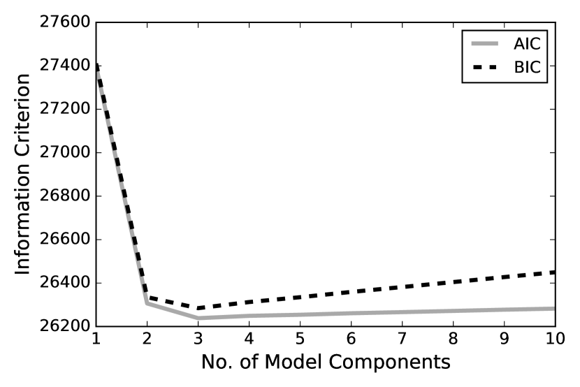
Figure 5 shows the velocity histogram of a sample of stars identified as MW stars using a simple cut of $\langle L_{i}\rangle$ $<-0.5$ (Section 3.2), along with the preferred Gaussian mixture model to the velocity distribution. Based on both the Aikake information criterion (AIC) and the Bayesian information criterion (BIC), the preferred number of Gaussian components for this dataset is three. Adding additional model components beyond three improves neither the AIC nor the BIC. The best-fit values of the mean velocity, dispersion, and mixture fraction for each component depends on the MW sample selection method (e.g., inclusion of the velocity diagnostic in computing $\langle L_{i}\rangle$, and/or inclusion of marginally identified MW stars, with $-0.5\leq$ $\langle L_{i}\rangle$ $<0$). However, the statistical preference for three Gaussian components, with decreasing mean velocity and increasing dispersion, is robust regardless of the MW sample selection: the minimum value in both the AIC and BIC metrics occurs with three Gaussian components for all MW samples tested.

The range in Galactic latitude spanned by the spectroscopic fields is substantial ($\sim$20^∘, Figure 1). The relative fraction of the three MW components is known to change over the full field of view of the survey (e.g., Martin et al., 2013), and it is reasonable to expect the mean velocity and dispersion of the disk components may change detectably as well. Ideally, the changing mixture of MW stellar populations over the field of the survey (e.g., with galactic latitude) could be included in our model, either empirically or through use of a physical model for the Galaxy.

A fundamental impediment to using a physical MW model, or a parameterized empirical model, is that the MW stars displayed in Figure 5 are not a simple and representative sampling of the MW components along the line of sight to M31. The MW stars with measured velocities are instead a complicated function of the target selection process, which was optimized to preferentially target M31 stars based on the available photometric data in each field, and the success of the cross-correlation routine used to measure velocities (dependent on both the observing conditions for each mask (affecting the SNR of the spectra) and the properties of the star itself (affecting the strength of absorption lines). We nevertheless explored drawing from the Besançon Galactic model (Robin et al., 2003) at the location of each field, limiting the model results only to those stars in the same apparent magnitude and color ranges as the targets in each field of the spectroscopic survey. We found that the velocity distribution of stars drawn from the Besançon model does not match the observed velocity distribution of MW stars in our survey.

Given the above considerations, we do not fix the MW component parameters based on fits to a selected sample of MW stars nor attempt a hierarchical fit including Galactic latitude or longitude. Rather, we fit all the parameters for the three MW components simultaneously with the parameters for the M31 components. As was assumed for the properties of the M31 halo, the properties of each of the three MW components is assumed to change relatively slowly and smoothly with spatial position within M31’s stellar halo (this is consistent with the Besancon Galaxy Model; Robin et al., 2003). Thus, the MW likelihood function is not field-dependent, and is simply

$$\mathscr{L}_{i}^{MW}=\sum_{j=1}^{N_{\rm MW}=3}f_{j}\mathscr{N}(v_{i}|\mu_{j},\sigma_{j}).$$ (12)

To ensure a normalized $\mathscr{L}_{i}^{MW}$, the sum of the fractions of the MW components is constrained to equal one:

$$\sum_{j=1}^{N_{\rm MW}=3}f_{j}=1.$$ (13)

Enforcing this normalization reduces the number of model parameters by one: the fraction of the third MW component is set to

$$f_{\rm MW3}=1-f_{\rm MW1}-f_{\rm MW2}.$$ (14)

4.2.3 Probability of M31 Membership

The probability of a given star $i$ being an M31 star ($p_{\rm M31}$, Equation 4) is primarily derived from the overall likelihood $\langle L_{i}\rangle$ that the star is an M31 star, which is based on multiple spectroscopic and photometric measurements (excluding the velocity diagnostic, Section 3.2). For each star, $\langle L_{i}\rangle$ is the logarithm of the odds ratio that the star is an RGB star at the distance of M31 or a MW dwarf star. Thus, the overall likelihood can be converted into a probability of M31 membership via

$$\frac{10^{\langle L_{i}\rangle}}{1+10^{\langle L_{i}\rangle}}.$$ (15)

The distribution of $\langle L_{i}\rangle$ values of stars in a field or radial region is in reality the superposition of two independent and overlapping distributions: that of MW stars and that of M31 stars. The MW (M31) $\langle L_{i}\rangle$ distribution has a tail that extends to positive (negative) $\langle L_{i}\rangle$ values (Gilbert et al., 2006, 2007, 2012). When one population (either the MW or M31) is strongly dominant, contamination (in $\langle L_{i}\rangle$ space) of the minority population by the tail of the distribution of the dominant population can be significant. For the present analysis, this is most concerning when considering M31’s outer halo, where MW stars outnumber M31 stars in the spectroscopic sample by 50:1 or more. If this effect is not accounted for, the tail of the MW star distribution, which has M31-like $\langle L_{i}\rangle$ values (greater than zero), results in the fit being driven to include MW stars as part of the M31 model. This will in turn drive the M31 mean velocity to larger values with increasing projected radius.

We therefore introduce a hyper-parameter $C$ to the prior probability of M31 membership to account for the possibility that a significant fraction of stars in a field may have $\langle L_{i}\rangle$-based probabilities that are not in line with their actual M31 or MW membership. Furthermore, since the density of M31 stars is the single largest driver in the amount of contamination in M31 samples, we add a field-dependent parameter, $\alpha_{sf}$, to the fit in fields with identified tidal debris, which typically have higher stellar densities than nearby halo fields without tidal debris features in M31’s halo. Thus,

$$p_{\rm M31}=\alpha_{sf}C\frac{10^{\langle L_{i}\rangle}}{1+10^{\langle L_{i}\rangle}},$$ (16)

and the probability that a star is an MW star is simply $1-p_{\rm M31}$. In fields without tidal debris features, $\alpha_{sf}\equiv 1$.

We restrict $\alpha_{sf}C$ to be less than or equal to one. This means it can only reduce the probability of M31 membership based on the empirical photometric and spectroscopic diagnostics. The greatest contrast between M31 and MW stellar density is in the outer M31 halo fields, where MW stars greatly outnumber M31 stars, and improperly categorized MW stars can have a significant effect on the M31 model parameters. In the innermost M31 halo fields included here, the converse is true: M31 stars outnumber MW stars, and improperly categorized M31 stars may affect the MW model parameters. However, the MW model parameters are nuisance parameters which we marginalize over: the MW model parameters have no direct physical interpretation due to our experimental setup (e.g., a varying spectroscopic selection function, averaging over Galactic latitude and longitude when binning the data based on projected radius from M31, and removing M31’s bulk motion from the stellar velocities). Moreover, under the assumption the kinematically hot halo is a well-mixed population, the fact that the tail of M31 stars with $\langle L_{i}\rangle$$<0$ contributes little to the M31 model will not introduce a systematic bias in the measurement of the M31 halo parameters.

4.3 Priors

As discussed above (Section 4.2), there are both field-independent and field-dependent model parameters. We discuss our choice of priors for each of these sets of parameters in turn.

4.3.1 Field Independent Parameters

The priors on the field-independent model parameters, which describe the M31 halo and the three MW components, are noninformative over the allowed range of the parameter with one exception. Table 1 lists the allowed range, choice of prior, and any additional constraints on the parameter implemented in the prior for the field-independent model parameters.

Table 1: Field-Independent Model Parameters.

Parameter	Description	Units	Allowed Range	Prior	Additional Constraints
M31 Parameters
$\mu_{\rm M31}$	Mean Velocity	km s-1	$-300<\mu_{\rm M31}<250$	normal	$\mu=-18$, $\sigma=5$
$\sigma_{\rm M31}$	Velocity Dispersion	km s-1	$5<\sigma_{\rm M31}<300$	scale free
MW Disk Component 1 Parameters
$\mu_{\rm MW1}$	Mean Velocity	km s-1	$150<\mu_{\rm MW1}<350$	uniform	$\mu_{\rm MW3}<\mu_{\rm MW2}<\mu_{\rm MW1}$
$\sigma_{\rm MW1}$	Velocity Dispersion	km s-1	$5<\sigma_{\rm MW1}<350$	scale free	$\sigma_{\rm MW3}<\sigma_{\rm MW2}<\sigma_{\rm MW1}$
$f_{\rm MW1}$	Fraction		$0<f_{\rm MW1}<1$	uniform	$f_{\rm MW1}+f_{\rm MW2}<1$
MW Disk Component 2 Parameters
$\mu_{\rm MW2}$	Mean Velocity	km s-1	$50<\mu_{\rm MW2}<350$	uniform	$\mu_{\rm MW3}<\mu_{\rm MW2}<\mu_{\rm MW1}$
$\sigma_{\rm MW2}$	Velocity Dispersion	km s-1	$5<\sigma_{\rm MW2}<350$	scale free	$\sigma_{\rm MW3}<\sigma_{\rm MW2}<\sigma_{\rm MW1}$
$f_{\rm MW2}$	Fraction		$0<f_{\rm MW2}<1$	uniform	$f_{\rm MW1}+f_{\rm MW2}<1$
MW Halo Parameters
$\mu_{\rm MW3}$	Mean Velocity	km s-1	$-200<\mu_{\rm MW3}<350$	uniform	$\mu_{\rm MW3}<\mu_{\rm MW2}<\mu_{\rm MW1}$
$\sigma_{\rm MW3}$	Velocity Dispersion	km s-1	$5<\sigma_{\rm MW3}<350$	scale free	$\sigma_{\rm MW3}<\sigma_{\rm MW2}<\sigma_{\rm MW1}$
Hyper-Parameter
$C$	affects prior probability		$0<C\leq 1$	uniform
	of M31 membership

The prior is uniform for the mean velocities and fractions of the total stellar population in the three MW components. The priors on the velocity dispersions of the MW components and the M31 halo go as $1/\sigma$, which is scale-free. A uniform prior is used for the hyper-parameter $C$ (Section 4.2.3)

The only informative prior on a field-independent model parameter is placed on the mean velocity of the M31 halo, for which we implement a normal prior with $\mu=-18$  km s^-1 and $\sigma=5$  km s^-1. This is based on the marginalized one-dimensional posterior distribution found for the M31 halo mean velocity resulting from performing a fit to all stars within 40 kpc of M31’s center, using the same fitting procedure described above, but assuming a uniform prior for the mean velocity of M31’s halo. This result is insensitive to the exact choice of projected radius used; fits including all stars within 30 kpc or 50 kpc of M31’s center return similar results. This is consistent with what has been found for the mean velocity of M31’s halo by Beaton et al. (in prep), who have used a separate kinematical analysis of the same spectroscopic dataset to measure the proper motion of M31.

We implement reasonable yet conservative minimum and maximum bounds on the range of each parameter, allowing considerable freedom for exploration of parameter space by the MCMC chains while eliminating clearly unphysical values. We also implement a hierarchy of mean velocities and velocity dispersions for the three MW components. This choice is informed by our physical understanding of the origin of the three MW components, as well as the results of Gaussian mixture model fits to samples of likely MW stars (Section 4.2.2).

4.3.2 Field Dependent Parameters

The field-dependent parameters describe the kinematically cold tidal debris features identified in individual fields. Table 4.3.2 lists the allowed range, choice of prior, and any additional constraints on the parameter implemented in the prior for the field-dependent model parameters.

The priors for the mean velocity and velocity dispersion of each tidal debris feature are set by the literature values for each component (Section 3.3, Table 4.3.2). We implement a normal prior on each mean velocity and velocity dispersion, using the published maximum-likelihood values and uncertainties on the maximum likelihood value of the parameter. The median RA and Dec of all stars in the field was used to transform the published mean velocity for each tidal debris feature to the Galactocentric frame, and to remove the bulk motion of M31. The published uncertainties on the mean velocities and velocity dispersions are in general not symmetric, and this is included in the prior. The range of allowed values has been bounded to be within 5 times the published upper and lower error on the maximum-likelihood value.

As for the field-independent parameters, additional constraints on the parameters are implemented in the prior. By construction, the sum of the fractions computed for the M31 components (halo and all tidal debris features present) in an individual field can not exceed unity. All components must have a fractional contribution greater than zero. In fields with more than one tidal debris feature, a hierarchy of values is enforced for the mean velocity of each tidal debris feature: the second kinematically cold component must have a mean velocity more negative than the first.

The parameter $\alpha$ (Section 4.2.3) is given a uniform prior and the freedom to vary over a significant range of values (0 to 10) to account for increased M31 stellar density due to tidal debris features, subject to the additional enforced constraint that $\alpha_{sf}C<=1$ (Section 4.2.3). In practice, $\alpha_{sf}$ is very close to one in fields with $R_{\rm proj}$ $<40$ kpc, and less than $\sim 2.5$ for fields with $R_{\rm proj}$ $>40$ kpc.

Table 2: Field-Dependent Model Parameters – Substructure Parameters and Priors.

Field	Parameter	Allowed Range	Prior			Additional	Reference
and Component			Form	Mean	Standard	Constraints
					Deviation
f115 KCC 1	$\mu_{\rm KCC1}$	$-49.00<\mu_{\rm KCC1}<77.00$	normal	$13.00$	$12.60$	…	1
	$\sigma_{\rm KCC1}$	$0.00<\sigma_{\rm KCC1}<104.70$	normal	$42.20$	$13.40$	…
	$f_{\rm KCC1}$	$0<f_{\rm KCC1}<1$	uniform	…	…	…
f116 KCC 1	$\mu_{\rm KCC1}$	$-98.39<\mu_{\rm KCC1}<85.11$	normal	$-10.89$	$18.35$	…	1
	$\sigma_{\rm KCC1}$	$0.00<\sigma_{\rm KCC1}<173.20$	normal	$51.20$	$19.70$	…
	$f_{\rm KCC1}$	$0<f_{\rm KCC1}<1$	uniform	…	…	…
H11 KCC 1	$\mu_{\rm KCC1}$	$-83.54<\mu_{\rm KCC1}<90.96$	normal	$4.46$	$17.45$	…	1
	$\sigma_{\rm KCC1}$	$0.00<\sigma_{\rm KCC1}<133.50$	normal	$55.50$	$14.15$	…
	$f_{\rm KCC1}$	$0<f_{\rm KCC1}<1$	uniform	…	…	…

f207 KCC 1 $\mu_{\rm KCC1}$ $-168.18<\mu_{\rm KCC1}<-76.68$ normal $-126.68$ $9.15$ … 2 $\sigma_{\rm KCC1}$ $0.00<\sigma_{\rm KCC1}<85.30$ normal $20.80$ $10.25$ … $f_{\rm KCC1}$ $0<f_{\rm KCC1}<1$ uniform … … … f207 KCC 2 $\mu_{\rm KCC2}$ $-262.48<\mu_{\rm KCC2}<-186.98$ normal $-225.48$ $7.55$ $\mu_{\rm KCC1}>\mu_{\rm KCC2}$ 2 $\sigma_{\rm KCC2}$ $0.00<\sigma_{\rm KCC2}<59.20$ normal $23.20$ $6.10$ … $f_{\rm KCC2}$ $0<f_{\rm KCC2}<1$ uniform … … $f_{\rm KCC1}+f_{\rm KCC2}<1$ f123 KCC 1 $\mu_{\rm KCC1}$ $-4.71<\mu_{\rm KCC1}<43.79$ normal $18.29$ $4.85$ … 1 $\sigma_{\rm KCC1}$ $0.00<\sigma_{\rm KCC1}<45.10$ normal $10.60$ $5.95$ … $f_{\rm KCC1}$ $0<f_{\rm KCC1}<1$ uniform … … … H13s KCC 1 $\mu_{\rm KCC1}$ $-116.99<\mu_{\rm KCC1}<-62.99$ normal $-89.99$ $5.40$ … 2 $\sigma_{\rm KCC1}$ $0.00<\sigma_{\rm KCC1}<50.00$ normal $17.00$ $6.75$ … $f_{\rm KCC1}$ $0<f_{\rm KCC1}<1$ uniform … … … H13s KCC 2 $\mu_{\rm KCC2}$ $-212.39<\mu_{\rm KCC2}<-168.89$ normal $-191.39$ $4.35$ $\mu_{\rm KCC1}>\mu_{\rm KCC2}$ 2 $\sigma_{\rm KCC2}$ $5.30<\sigma_{\rm KCC2}<41.30$ normal $21.30$ $3.60$ … $f_{\rm KCC2}$ $0<f_{\rm KCC2}<1$ uniform … … $f_{\rm KCC1}+f_{\rm KCC2}<1$ f115 KCC 1 $\mu_{\rm KCC1}$ $-49.24<\mu_{\rm KCC1}<76.76$ normal $12.76$ $12.60$ … 1 $\sigma_{\rm KCC1}$ $0.00<\sigma_{\rm KCC1}<104.70$ normal $42.20$ $13.40$ … $f_{\rm KCC1}$ $0<f_{\rm KCC1}<1$ uniform … … … f135 KCC 1 $\mu_{\rm KCC1}$ $-59.97<\mu_{\rm KCC1}<85.03$ normal $25.03$ $14.50$ … 1 $\sigma_{\rm KCC1}$ $0.00<\sigma_{\rm KCC1}<103.60$ normal $30.10$ $11.85$ … $f_{\rm KCC1}$ $0<f_{\rm KCC1}<1$ uniform … … … f135 KCC 2 $\mu_{\rm KCC2}$ $-320.97<\mu_{\rm KCC2}<-5.97$ normal $-150.97$ $31.50$ $\mu_{\rm KCC1}>\mu_{\rm KCC2}$ 1 $\sigma_{\rm KCC2}$ $0.00<\sigma_{\rm KCC2}<191.00$ normal $55.50$ $23.80$ … $f_{\rm KCC2}$ $0<f_{\rm KCC2}<1$ uniform … … $f_{\rm KCC1}+f_{\rm KCC2}<1$ a3 KCC 1 $\mu_{\rm KCC1}$ $-169.25<\mu_{\rm KCC1}<-118.75$ normal $-144.75$ $5.05$ … 2 $\sigma_{\rm KCC1}$ $0.30<\sigma_{\rm KCC1}<39.80$ normal $16.80$ $3.95$ … $f_{\rm KCC1}$ $0<f_{\rm KCC1}<1$ uniform … … … and9 KCC 1 $\mu_{\rm KCC1}$ $-63.57<\mu_{\rm KCC1}<20.93$ normal $-30.57$ $8.45$ … 2 $\sigma_{\rm KCC1}$ $0.00<\sigma_{\rm KCC1}<67.60$ normal $12.60$ $7.90$ … $f_{\rm KCC1}$ $0<f_{\rm KCC1}<1$ uniform … … … and1 KCC 1 $\mu_{\rm KCC1}$ $-31.34<\mu_{\rm KCC1}<39.66$ normal $5.66$ $7.10$ … 2 $\sigma_{\rm KCC1}$ $0.00<\sigma_{\rm KCC1}<51.20$ normal $8.20$ $6.55$ … $f_{\rm KCC1}$ $0<f_{\rm KCC1}<1$ uniform … … … and1 KCC 2 $\mu_{\rm KCC2}$ $-145.14<\mu_{\rm KCC2}<-25.14$ normal $-87.14$ $12.00$ $\mu_{\rm KCC1}>\mu_{\rm KCC2}$ 2 $\sigma_{\rm KCC2}$ $0.00<\sigma_{\rm KCC2}<96.80$ normal $30.30$ $10.95$ … $f_{\rm KCC2}$ $0<f_{\rm KCC2}<1$ uniform … … $f_{\rm KCC1}+f_{\rm KCC2}<1$ a13 KCC 1 $\mu_{\rm KCC1}$ $-63.67<\mu_{\rm KCC1}<54.33$ normal $-5.67$ $11.80$ … 2 $\sigma_{\rm KCC1}$ $0.00<\sigma_{\rm KCC1}<91.20$ normal $32.20$ $11.20$ … $f_{\rm KCC1}$ $0<f_{\rm KCC1}<1$ uniform … … … m4 KCC 1 $\mu_{\rm KCC1}$ $10.38<\mu_{\rm KCC1}<64.38$ normal $34.88$ $5.40$ … 2 $\sigma_{\rm KCC1}$ $0.00<\sigma_{\rm KCC1}<36.60$ normal $6.60$ $4.45$ … $f_{\rm KCC1}$ $0<f_{\rm KCC1}<1$ uniform … … … m4 KCC 2 $\mu_{\rm KCC2}$ $-88.12<\mu_{\rm KCC2}<-40.12$ normal $-65.62$ $4.80$ $\mu_{\rm KCC1}>\mu_{\rm KCC2}$ 2 $\sigma_{\rm KCC2}$ $0.00<\sigma_{\rm KCC2}<37.40$ normal $11.40$ $4.65$ … $f_{\rm KCC2}$ $0<f_{\rm KCC2}<1$ uniform … … $f_{\rm KCC1}+f_{\rm KCC2}<1$ R06A220 KCC 1 $\mu_{\rm KCC1}$ $-86.33<\mu_{\rm KCC1}<-56.33$ normal $-71.33$ $3.00$ … 3 $\sigma_{\rm KCC1}$ $0.00<\sigma_{\rm KCC1}<19.60$ normal $6.10$ $2.20$ … $f_{\rm KCC1}$ $0<f_{\rm KCC1}<1$ uniform … … … each field, $\alpha_{sf}$ $0<\alpha_{sf}<10$ uniform … … $\alpha_{sf}C\leq 1$ … $sf$, above

4.4 Sampling the Posterior Probability Distribution with MCMC

Following Bayes’ theorem, we multiplied the likelihood of the data given the model (Section 4.2) with the prior distribution for each parameter in the model (Section 4.3) to compute the likelihood of the model given the data. We used MCMC methods to efficiently sample the parameter space, and marginalized over all model parameters to obtain posterior probability distributions for each parameter of interest.

We sampled the posterior probability distributions for all of the model parameters described above using the open-source emcee python package (Foreman-Mackey et al., 2013a, b), which provides an efficient implementation of the Goodman & Weare (2010) Affine Invariant MCMC Ensemble sampler. The number of parameters in the model is dependent on the number of tidal debris features (Section 4.2), and thus varies based on the spectroscopic fields included in the fit. In order to balance the required computational resources with the final number of independent samples, the number of MCMC chains was set to be at least ten times, and no more than 20 times, the number of model parameters included in the fit. However, if that value was less than 300, we instead ran the MCMC analysis with a minimum threshold of 300 chains (Table 3).

Chains were initialized using a random, uniform distribution over the valid parameter space implemented in the prior for each parameter. The chains were run for a minimum of 12,000 steps. The marginalized one- and two-dimensional projections of the posterior probability distributions are computed by drawing the values of the model parameters from the last half of each MCMC chain. The choice to use the first half of the chains as the burn-in period was made as a conservative choice that could be applied uniformly to all chains, for all radial bins. The autocorrelation time of the chains stabilized by half way through the chain for all the parameters considered in the following analysis. In most cases, the autocorrelation time stabilized well before the half way point.

Post-burn in, the chains for all parameters were inspected to ensure they had settled to an equilibrium. The parameter values and confidence limits as a function of the number of steps in the chain were also inspected to ensure stability had been achieved. The chains were run long enough to supply a sufficient number of independent samples (estimated using the autocorrelation length) to estimate the uncertainties on the parameters of interest to a level of $\sim 1$%.

The results of the MCMC analysis presented below define the best estimate for each parameter as the 50th percentile of the one-dimensional posterior probability distribution, marginalized over all other model parameters. The associated uncertainties on the best estimates are the 16th and 84th percentiles of the posterior probability distributions.

5 The M31 Halo Velocity Dispersion as a Function of Radius

To characterize the change of the velocity dispersion of M31’s halo with projected radius from M31’s center, the full spectroscopic dataset was split into multiple radial bins. The MCMC analysis described in Section 4 was completed for each radial bin. The bounds of each radial bin were chosen to minimize the number of fields that span two radial bins, while ensuring that at least 100 stars more likely to be M31 stars than MW stars based on their $\langle L_{i}\rangle$ values (Section 3.2, not including the velocity diagnostic) were present in each bin. Table 3 lists the total number of stars in each bin, as well as the number of stars likely to be M31 stars (Section 3.2). A final consideration was including at least one field without identified tidal debris features in each bin; this removed degeneracies between the field-independent and field-dependent model hyper-parameters $C$ and $\alpha_{sf}$ (Section 4.2.3).

Figure 6: The stellar velocity distribution ($v_{\rm pec}$, Section 4.1) in each of the seven radial bins. Overlaid are 150 samples of the parameterized velocity distribution, drawn from the MCMC chain. The blue curves include only the M31 components, while the green curves include all M31 and MW components. Observed line of sight velocities have been transformed to the Galactocentric frame, and the bulk motion of M31 has been removed (Section 4): a star with no peculiar velocity relative to M31’s bulk motion will have $v=0$  km s^-1.

Table 3: Parameters Describing the Velocity Distribution of M31 Halo Stars.

$R_{\rm min}$	$R_{\rm max}$	No.	No. M31	No.	No.	Mean	Velocity	Fields with
(kpc)	(kpc)	Stars	Stars	Model	MCMC	Velocity	Dispersion	Substructure
				Parameters	Chains	$\mu_{\rm M31}$	$\sigma_{\rm M31}$
						( km s-1)	( km s-1)
8.2	14.1	617	525	23	460	$-16.5^{+4.3}_{-4.5}$	$108.2^{+6.8}_{-6.6}$	f115, f116, H11
14.1	24	896	697	40	400	$-20.6^{+4.4}_{-4.2}$	$98.1^{+5.3}_{-5.0}$	f207, f123, H13s, f115, f135
24	40	382	240	19	380	$-18.9^{+4.4}_{-4.4}$	$98.0^{+7.2}_{-6.6}$	a3, and9
40	63	589	202	29	436	$-17.1^{+4.9}_{-4.8}$	$93^{+11}_{-10}$	and1, a13, m4
63	90	1068	247	15	300	$-11.8^{+4.7}_{-4.7}$	$76.0^{+8.6}_{-7.6}$	R06A220
90	130	1013	202	11	300	$-17.4^{+4.8}_{-4.8}$	$88^{+13}_{-10}$
130	200	684	104	11	300	$-17.2^{+5.0}_{-5.0}$	$92^{+40}_{-31}$

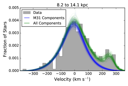
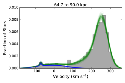
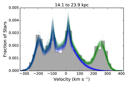
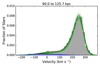
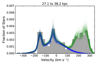
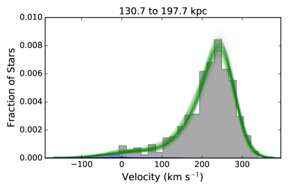
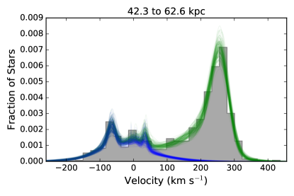
Figure 6 shows the velocity distribution of stars in each radial bin, along with a visualization of 150 randomly drawn samples from the MCMC chain overlaid. As the overall ratio of MW and M31 stars is not a parameter in the mixture model, the fraction of stars with posterior probabilities of M31 membership greater than 0.5 is used as the M31 fraction. This is done purely to allow the visualization of the models in Figure 6.

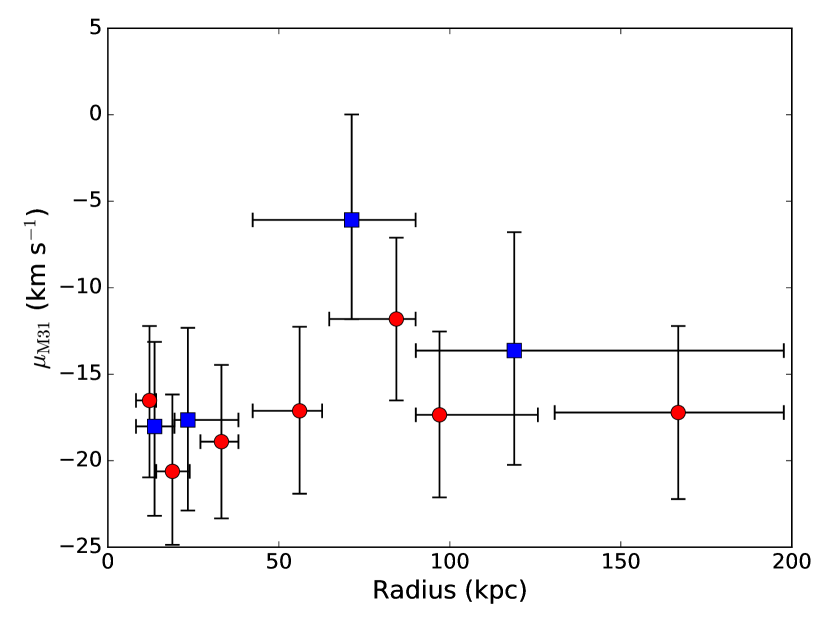
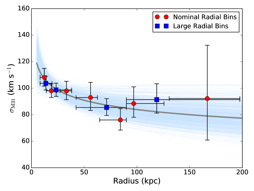
The velocity dispersion of the kinematically hot M31 halo component is well constrained in all but the outermost radial bin. However, only a weak gradient in the M31 halo velocity dispersion with projected radius is seen (Figure 7). For each radial bin, Table 3 lists the 50th percentile of the marginalized one-dimensional posterior probability distribution of the field-independent M31 model parameters, along with the estimated uncertainties based on the 16th and 84th percentiles. Marginalized one- and two- dimensional posterior probability distributions for all field-independent and field-dependent model parameters are shown in the Appendix.

The uncertainties listed in Table 3 are based solely on the results of the MCMC analysis, and do not include velocity measurement (Section 2.3) or transformation (Section 4.1) uncertainties. Assuming the measured velocity dispersion is a combination of the intrinsic velocity dispersion of halo stars, the velocity measurement uncertainties, and the uncertainties in the velocity transformations (all added in quadrature), we can estimate the impact of these uncertainties on our measurement of the velocity dispersion. For most radial bins, the typical values of these uncertainties will inflate the measured dispersion by only a few tenths of a  km s^-1, which is only $\sim 10$% of the estimated uncertainties from the MCMC method. The uncertainties in the transformations are expected to lead to larger effects in the outer radial bins than in the inner radial bins, as fields in the outer bins are often separated by many degrees on the sky (Figure 1). The maximum effect from the velocity transformations is estimated to introduce an uncertainty on the order of $8$ – $10$  km s^-1; this would be the maximum effect for the outermost radial bin. Nevertheless, we can use this to provide a conservative upper bound: using these values, we find that the measured dispersion is inflated by only $\sim 1$ – 1.3  km s^-1, which is $<2$% of the measured dispersion in the three outermost radial bins, and is still a small fraction ($\lesssim 15$%) of the estimated uncertainties from the MCMC method in these bins.

Figure 7: Field independent M31 model parameters as a function of projected radius from M31’s center [halo mean velocity (upper panel; $v_{\rm pec}$, Section 4.1) and halo velocity dispersion (lower panel)]. Each point is placed at the median projected radius of all stars in the radial bin, with the error bar showing the full range of radii of the stars in the bin. The model parameter value is the 50th percentile of the marginalized one-dimensional posterior probability distribution, and the errorbar on the parameter value shows the span of the 16th and 84th percentiles. The velocity dispersion of M31’s halo decreases only mildly with radius. In addition to the 7 nominal radial bins, this figure also shows the results when the data is binned into 4 large radial bins (large blue squares); the results are consistent with the smaller radial bins used in the analysis.

5.1 Parameterization of the Velocity Dispersion of M31’s Halo with Radius

Figure 8: A representation of the probability distribution of the halo mean velocity (upper panel; $v_{\rm pec}$, Section 4.1) and velocity dispersion (lower panel) of M31’s stellar halo as a function of projected radius. The M31 halo velocity mean and dispersion from each MCMC sample was randomly assigned to the radius of a star in that radial bin. The resulting data were then randomly sampled, drawing a total of $1.5\times 10^{6}$ samples for each radial bin. Purple represents the regions of low probability density while yellow represents the regions of highest probability density. White regions of the plot indicate where the probability density is zero, as well as where there are gaps in the radial coverage of the spectroscopic dataset.

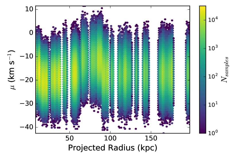
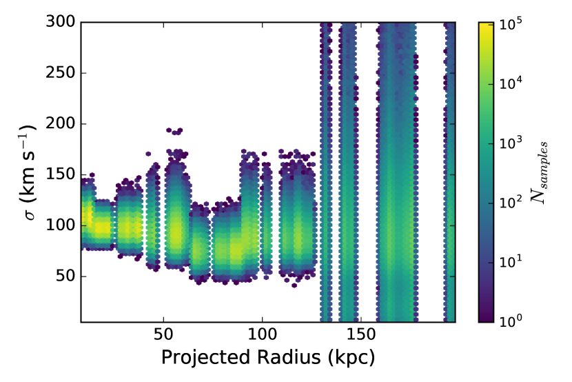
To parameterize the change in the velocity dispersion of M31’s halo with projected radius, we leverage the one-dimensional posterior probability distributions, i.e., those that are marginalized over all other model parameters. A visualization of the posterior probability distributions for the M31 halo velocity dispersion as a function of radius is shown in Figure 8. In this representation, it is very clear that the halo dispersion in outermost radial bins is poorly constrained: the probability distribution extends over a large range of values, and does not have a prominent peak.

We randomly sample the marginalized, one-dimensional posterior probability distributions of the M31 halo dispersion in each radial bin to parameterize the change in the velocity dispersion of M31’s halo with radius. We fit a power-law of the form

$$\sigma=\sigma_{0}\,(R_{\rm med}/R_{\rm 0})^{-\gamma},$$ (17)

where the power-law is normalized at the projected radius $R_{\rm 0}$. We set $R_{\rm 0}=30$ kpc, which is the scale radius chosen for the analysis of the M31 GC dispersion profile in Veljanoski et al. (2014). $R_{\rm med}$ is the median value of the projected radii of all stars in each radial bin.

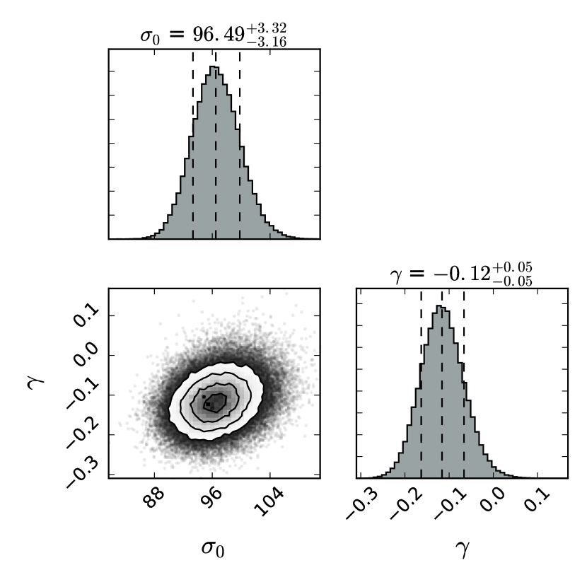
We make 10,000 random draws (with replacement) from the one-dimensional posterior probability distributions for the M31 halo velocity dispersion in the first 6 radial bins, and perform a least-squares fit on each draw to determine the power-law parameters $\sigma_{0}$ and $\gamma$. The resulting distribution functions of $\sigma_{0}$ and $\gamma$ provide estimates of the most likely values and uncertainty on each parameter (Figure 9). The 50th percentile values, with uncertainties estimated from the 16th and 84th percentiles of the distributions, are $\gamma=-0.12\pm 0.05$ and $\sigma_{0}=96.5^{+3.3}_{-3.2}$  km s^-1. A random drawing of 1000 of these power-law fits is shown in Figure 10. This parameterization confirms the likely existence of a weak gradient in the velocity dispersion with projected radius: only a small percentage of the fits are consistent with a flat or increasing dispersion with radius.

The uncertainties in the power-law slope are estimated based on the method, and do not include formal propagation of uncertainties such as those in the velocity measurements or transformations. However, as discussed in Section 5, these uncertainties are estimated to have a minimal effect on the measured velocity dispersions, and this will propagate to a minimal effect on the power-law slope uncertainties. We discuss the effect of modeling choices on the power-law slope below (Section 5.2).

Figure 9: One- and two-dimensional distributions of the best-fit power-law parameters describing the change in the velocity dispersion of M31’s halo with projected radius. Each point comes from fitting a power-law to random draws from the M31 halo velocity dispersion posterior probability distributions in all but the outermost radial bin (Figure 8).

Figure 10: Same as the lower panel of Figure 7, with the power-law fits of the velocity dispersion of M31’s halo as a function of projected radius overlaid. The light blue curves show a subset of the power-law fits to 10000 random draws from the marginalized one-dimensional posterior distribution functions for the M31 halo velocity dispersion in each of the first six radial bins. The dark gray curve shows a power-law composed of the 50th percentile values of the normalization and slope distributions.

5.2 Sensitivity to Modeling Choices

We made several choices regarding both the data and the modeling with the potential to influence the results. We performed alternative fits to explore the impact of these choices on the measured dispersion profile.

We instituted a strong prior probability that stars significantly bluer than the most metal-poor red giant branch isochrone are MW stars along the line of sight, rather than M31 red giant branch stars, by assigning them very negative $\langle L_{i}\rangle$ values of $-5$. This places them on the tail end of the distribution of MW stars in $\langle L_{i}\rangle$ space, and is consistent with the approach taken in previous papers. However, we also ran the above analysis after assigning less negative $\langle L_{i}\rangle$ values to these stars, based on the $\langle L_{i}\rangle$ distribution of stars classified as MW stars: they were assigned an $\langle L_{i}\rangle$ value one sigma below the mean $\langle L_{i}\rangle$ of all MW stars. This still places them firmly as having a high probability of being MW stars, but is a less draconian $\langle L_{i}\rangle$ assignment. This resulted in no appreciable difference in the power-law parameters found for the stellar halo dispersion profile ($\sigma_{0}=96.5^{+3.3}_{-3.2}$  km s^-1, $\gamma=-0.12\pm 0.05$).

We also explored fits with variations on the M31 halo mean velocity parameter, including a delta prior on the mean velocity at M31’s systemic velocity (0  km s^-1). This also made little difference in the power-law parameters, resulting in values consistent with those found in the nominal fit ($\sigma_{0}=100.0^{+3.4}_{-3.3}$  km s^-1, $\gamma=-0.09\pm 0.05$). Using a normal prior on the M31 halo mean velocity parameter, but centered at M31’s systemic velocity and with a width of $\sigma=10$ km s^-1, resulted in a slightly flatter halo velocity dispersion profile, but with power-law parameters statistically consistent (within one sigma) with the nominal fit ($\sigma_{0}=99.3^{+3.5}_{-3.3}$  km s^-1, $\gamma=-0.07\pm 0.05$).

Relaxing the boundary constraints on the substructure prior (allowing values within $\pm 10$ times the uncertainties on the published best-fit values) also did not result in a significant change in the power-law parameters ($\sigma_{0}=96.3^{+3.4}_{-3.2}$   km s^-1, $\gamma=-0.11\pm 0.05$).

Finally, we have measured the power-law based on projected radii calculated using a distance modulus to M31 of $24.47^{m}$ (Section 1). If instead we use a distance modulus of $24.38^{m}$, this results in an $\sim 4$% difference in the estimated projected radii in kpc. The primary effect of assuming a different distance modulus on the estimated power-law slope is easy to compute by simply recalculating the power-law after recomputing the median projected radius for each bin. The resulting power-law parameters ($\sigma_{0}=96.1\pm 3.3$  km s^-1, $\gamma=-0.12\pm 0.05$) are fully consistent with the nominal fit.

5.3 Discussion

Only one other measurement of the dispersion profile of stars in M31’s halo over a large range of radii has been attempted, by Chapman et al. (2006, Section 1). The Chapman et al. fields were primarily within 40 kpc of M31’s center and almost exclusively located on M31’s disk. This required the application of strict window functions to the velocity distribution to remove M31 disk stars and MW stars. This early analysis could not account for recent discoveries of rotation in M31’s inner spheroid ($v_{\rm rot}\sim 50$  km s^-1; Dorman et al., 2012) and the relatively large line of sight velocity dispersion of disk RGB stars ($\sigma_{v}=90$ km s^-1; Dorman et al., 2015), both of which will affect the interpretation of the relative mix of stellar populations assumed to fall within the Chapman et al. velocity window functions. Nevertheless, the results are consistent with the recent measurements of Veljanoski et al. (2014), who measured the dispersion profile of M31 halo globular clusters (GCs) over a large radial range. The study by Veljanoski et al. (2014) sampled projected radii of 25 – 145 kpc, and while it includes many less tracer objects (72 beyond 30 kpc), there are fewer populations from which these objects are drawn: all are firmly in the M31 system. After accounting for the rotation observed in the GC system, Veljanoski et al. measured a power-law dispersion profile with both a larger value of $\sigma_{0}$ and a steeper power-law slope, $-0.45$, with only a 1% posterior probability of $\gamma=0$. While Veljanoski et al. find clear evidence of coherent velocity patterns amongst groups of GCs that are spatially correlated with tidal debris features, the analysis did not account for this. The ability to do so is an advantage of using much more abundant halo RGB stars as tracers of the halo.

Measurements of the velocity dispersion of MW halo stars have found a sharp decrease in the velocity dispersion in the inner regions of the MW halo from $\sim 150$ to 100 km s^-1 over the inner 20 kpc, settling to a relatively flat dispersion profile at large radii, with measurements of $\sigma_{r}\sim 100$  km s^-1 from $\sim 20$ – 80 kpc (Battaglia et al., 2005; Xue et al., 2008; Bond et al., 2010; Brown et al., 2010; Kafle et al., 2012; Deason et al., 2012; Kafle et al., 2014). A graphical summary of the MW’s velocity dispersion profile can be found in Bland-Hawthorn & Gerhard (2016).

M31 also appears to have a sharply decreasing velocity dispersion in the inner regions (Dorman et al. (2012) measured a velocity dispersion of $140$  km s^-1 at $R_{\rm proj}$$=7~{}kpc$ in M31), followed by a relatively flat dispersion to large radii. However, the reader should note that the MW profiles measure primarily the radial velocity of MW halo stars. Given the large spread of the SPLASH spectroscopic fields on the sky, the M31 line of sight velocity dispersion profile measures a combination of the stars’ tangential and radial velocities in the M31 coordinate frame, with the relative contributions changing with field position.

To date, there have been few analyses of the velocity dispersion profiles of MW- or M31-like stellar halos in $\Lambda$CDM simulations (one example is Abadi et al., 2006). The stellar density profiles, substructure characteristics, and metallicity profiles of the M31 and MW halos have proven to be useful constraints and checks on $\Lambda$CDM simulations of stellar halo formation, and comparisons of the simulations to observations have provided insight into the physical origins of the stellar halos of M31 and the MW (e.g., Font et al., 2006, 2008; Zolotov et al., 2010; Font et al., 2011; McCarthy et al., 2012; Gilbert et al., 2012, 2014). We expect future comparisons of the observed MW and M31 velocity dispersion profiles with simulated halos will yield further insights into the origins of stellar halos.

6 Conclusion

We modeled the velocity distribution of more than 5000 stars observed in M31 halo fields as part of the SPLASH survey, including all major MW and M31 components in the halo fields. Photometric and spectroscopic information on likely MW or M31 membership for each star was incorporated into the Gaussian mixture model as a prior probability. Tidal debris features in M31 halo fields were included in the model, and the marginalized posterior distributions for each are presented in the appendix.

Marginalizing over all model parameters, we parameterized the dispersion of stars in M31’s halo as a function of projected radius. The dispersion of M31’s halo stars is found to decrease only mildly with projected radius, over a radial range of 9 to 100 kpc. Our measurement finds a significantly flatter profile with radius than that measured for M31’s globular cluster population. The measurement of the velocity dispersion profile is the first step towards using halo stars as tracers of M31’s mass. In future work, the dispersion M31’s halo stars will be used to model M31’s total mass distribution.

Appendix A Posterior Probability Distributions of the Field-Independent Parameters

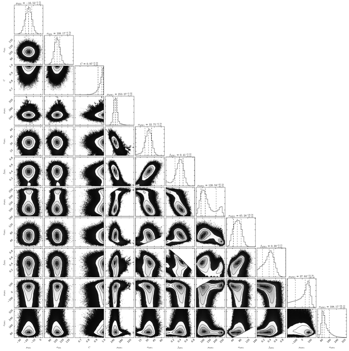
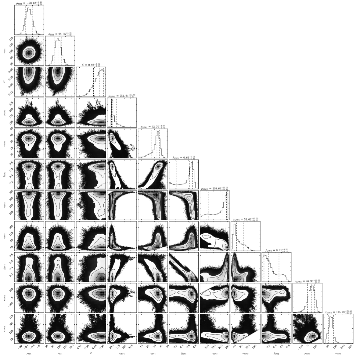
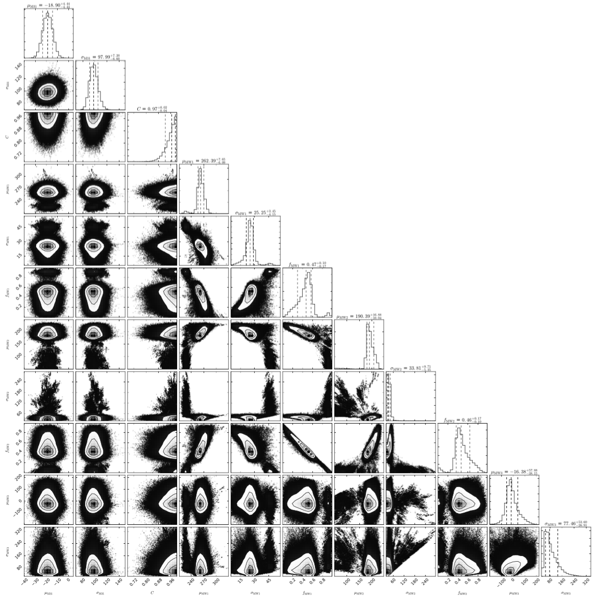
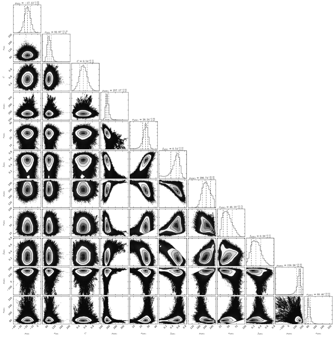
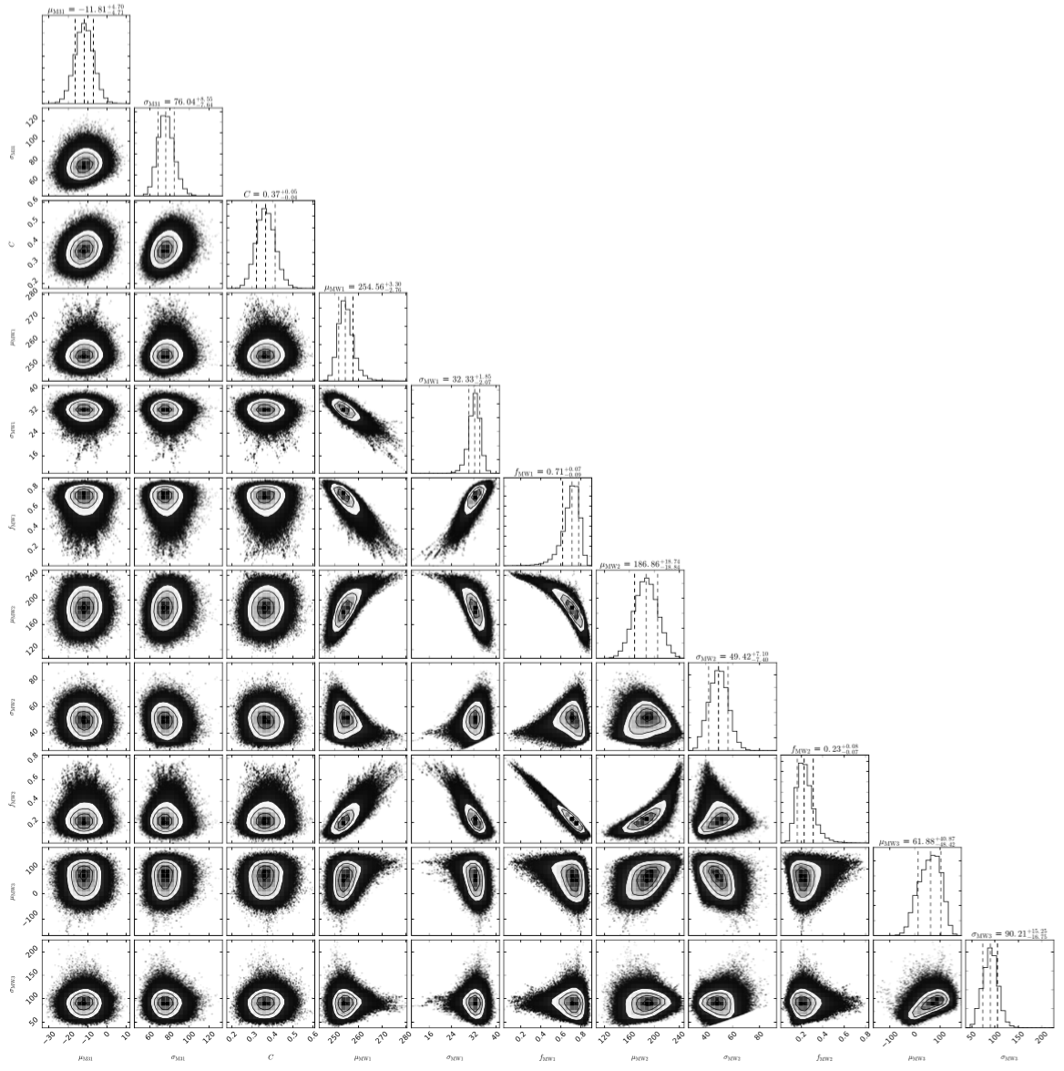
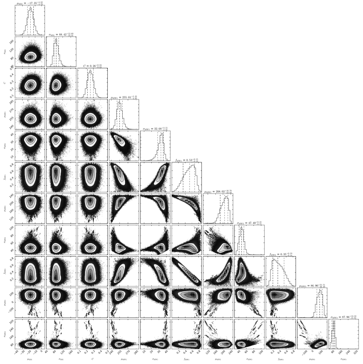
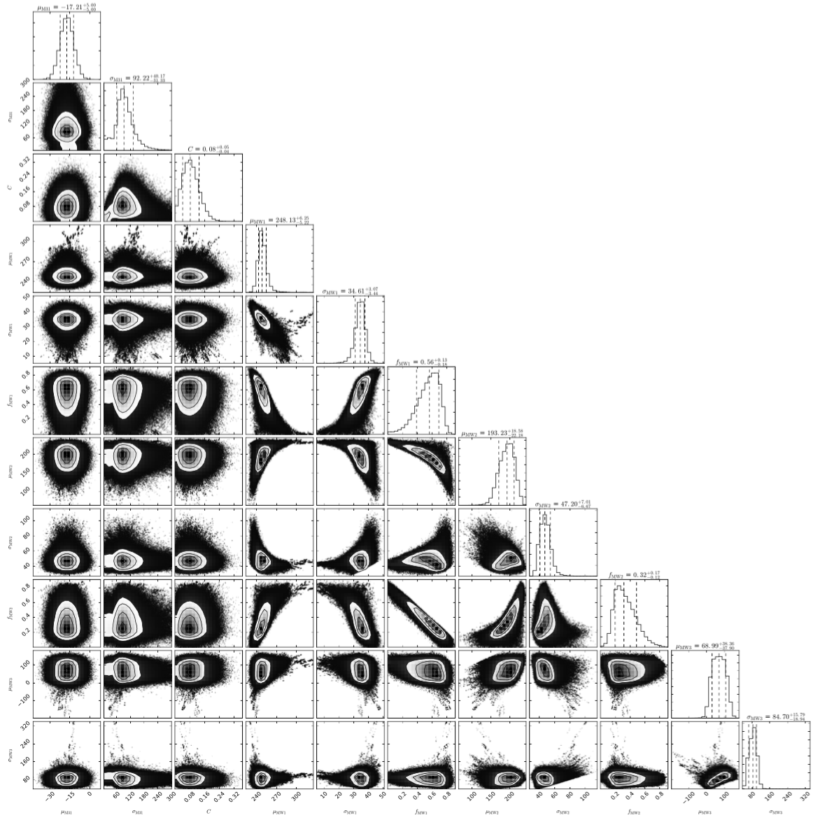
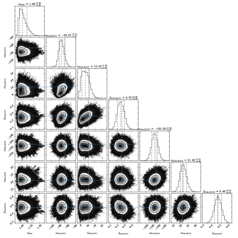
Figures 11 through 17 show the marginalized one- and two-dimensional posterior probability distributions for the field-independent model parameters in each radial bin. The model parameters describing the M31 halo component are well constrained in all but the outermost radial bin, where the number of M31 stars in the dataset is very low. Conversely, in the inner radial bins, the number of MW stars in the dataset is small, and the constraints on the model parameters describing the MW components is poor. The constraints on the model parameters describing the MW components increase in the fits at large projected radius, where the dataset contains significantly more MW stars. The results for the MW component model parameters reflect only the distribution of spectroscopic targets, and are dependent on the spectroscopic target selection functions. Thus, they should not be used as general measurements of the physical properties of the MW velocity distribution towards M31.

Figure 11: Marginalized one- and two-dimensional posterior probability distributions for the field-independent model parameters (Section AA) in the first radial bin ($8.2\leq$ $R_{\rm proj}$ $<14.1$ kpc). The distributions are computed using the values of the model parameters in the half of each of the MCMC chains. The 16th, 50th, and 84th percentiles of the marginalized one-dimensional distributions are marked by dashed lines, and these values are listed for each parameter at the top of each column. In the two-dimensional distribution panels, contours are displayed at levels of 0.5, 1, 1.5, and 2$\sigma$. This figure and those that follow were created using the open source python package corner (Foreman-Mackey et al., 2016; Foreman-Mackey, 2016).

Figure 12: Same as Figure 11 for the second radial bin ($14.1\leq$ $R_{\rm proj}$ $<24$ kpc).

Figure 13: Same as Figure 11 for the third radial bin ($24\leq$ $R_{\rm proj}$ $<40$ kpc).

Figure 14: Same as Figure 11 for the fourth radial bin ($40\leq$ $R_{\rm proj}$ $<63$ kpc).

Figure 15: Same as Figure 11 for the fifth radial bin ($63\leq$ $R_{\rm proj}$ $<90$ kpc).

Figure 16: Same as Figure 11 for the sixth radial bin ($90\leq$ $R_{\rm proj}$ $<130$ kpc).

Figure 17: Same as Figure 11 for the seventh radial bin ($130\leq$ $R_{\rm proj}$ $<200$ kpc).

Appendix B Posterior Probability Distributions of the Field-Dependent Parameters

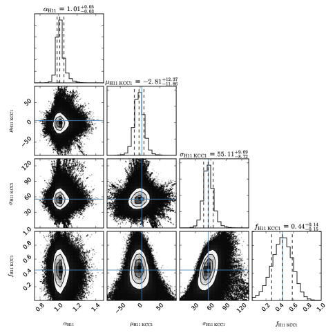
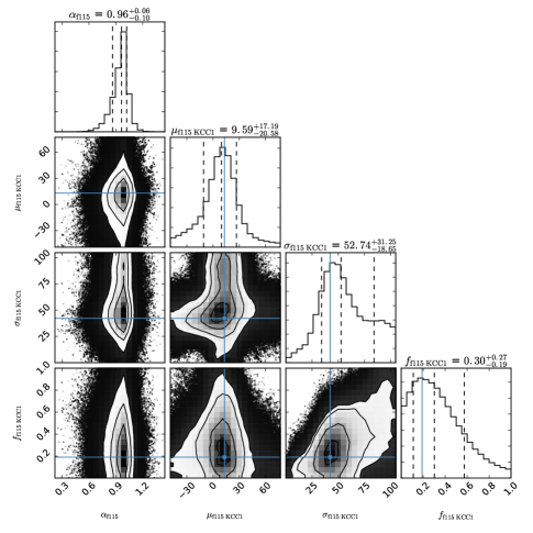
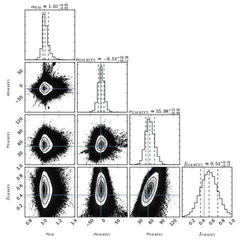
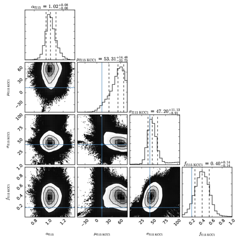
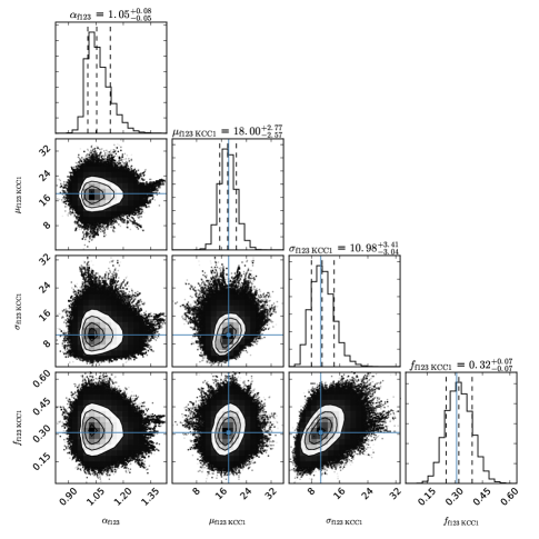
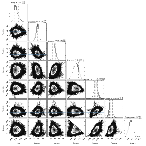
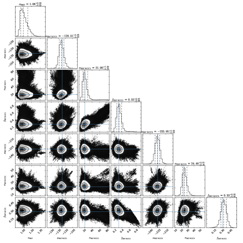
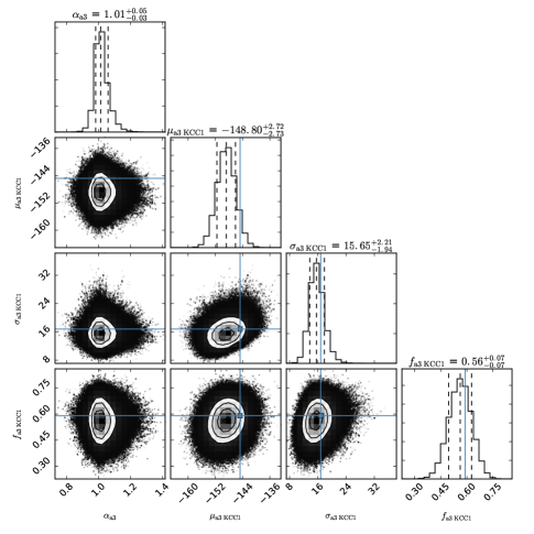
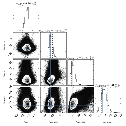
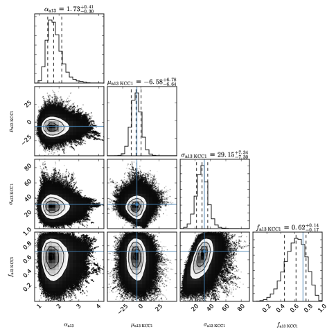
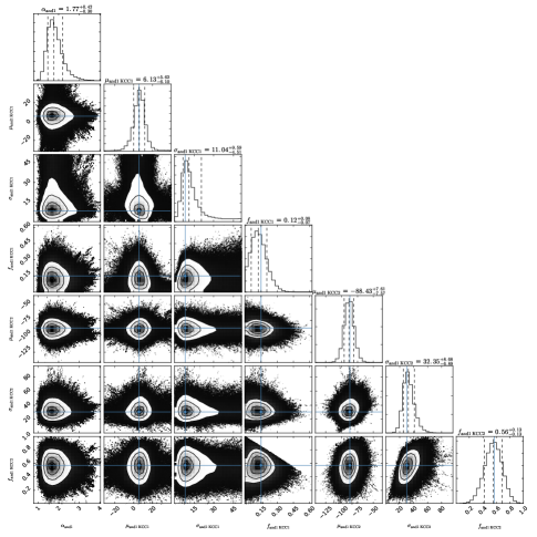
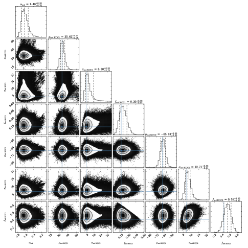
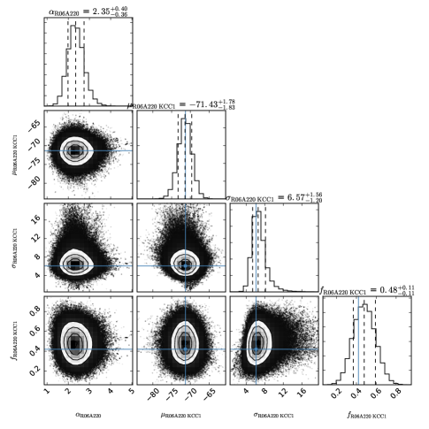
Figures 18 through 23 show the marginalized one- and two-dimensional posterior probability distributions for the field-dependent model parameters in each radial bin. Each of these features were originally identified and characterized using maximum-likelihood, multi-Gaussian fits to the M31 stars in their respective spectroscopic field (Section 3.3). The results for the mean velocity, velocity dispersion, and fraction of M31 stars in each component are listed in Table B.

Most of the tidal debris features are well constrained when fit within the full model (all M31 plus MW components). However, a few of the model parameters for individual tidal features show evidence of multi-modality or lower-probability tails in the posterior distributions, hinting that there may be additional kinematical structure in these fields (e.g., fields f207 and m4 in Figures 20 and 22, respectively). In a few others, the two-dimensional posterior probability distributions are relatively poorly constrained, indicating that the kinematically-identified feature may not be robust (e.g., the second component in field ‘f135’, Figure 19).

The spectroscopic field ‘f115’ is the only field containing a tidal debris feature that was split between radial bins, with the majority of f115 stars falling in the second radial bin rather than the first. The original, maximum-likelihood Gaussian fits to the velocity distribution of M31 stars in this field did not require the presence of an additional component to the kinematically hot M31 halo component (Gilbert et al., 2007). However, it is in the middle of the region that Gilbert et al. (2007) found to be contaminated by a large shell feature (the Southeast Shelf), which can be connected to M31’s most significant tidal debris feature, the Giant Southern Stream (Gilbert et al., 2007; Fardal et al., 2007, 2012). Therefore, we include a single tidal debris feature in the likelihood function for this field, with the prior on the tidal debris feature model parameters based on the multi-Gaussian fit to all of the Southeast Shelf spectroscopic fields (Gilbert et al., 2007).

Table 4: Field-Dependent Model Parameter Results.

f207 KCC 1 $-128.3^{+5.4}_{-4.6}$ $-427.2$ $21.0^{+7.4}_{-4.8}$ $0.318^{+0.074}_{-0.062}$ f207 KCC 2 $-226.0^{+4.4}_{-4.4}$ $-524.9$ $24.5^{+3.9}_{-3.2}$ $0.331^{+0.052}_{-0.051}$ f123 KCC 1 $18.0^{+2.8}_{-2.6}$ $-279.7$ $11.0^{+3.4}_{-3.0}$ $0.322^{+0.073}_{-0.069}$ H13s KCC 1 $-93.8^{+2.9}_{-2.5}$ $-392.1$ $13.2^{+4.5}_{-4.1}$ $0.254^{+0.050}_{-0.046}$ H13s KCC 2 $-192.6^{+2.6}_{-2.5}$ $-490.9$ $21.9^{+2.2}_{-2.0}$ $0.483^{+0.042}_{-0.042}$ f115 KCC 1 $53^{+14}_{-23}$ $-245$ $47.2^{+11.1}_{-8.9}$ $0.40^{+0.14}_{-0.14}$ f135 KCC 1 $24.0^{+8.8}_{-9.3}$ $-274.0$ $35.7^{+8.1}_{-6.9}$ $0.43^{+0.11}_{-0.12}$ f135 KCC 2 $-143^{+24}_{-23}$ $-441$ $64^{+15}_{-14}$ $0.36^{+0.11}_{-0.11}$   24 to 40 kpc    a3 KCC 1 $-148.8^{+2.7}_{-2.7}$ $-444.6$ $15.7^{+2.2}_{-1.9}$ $0.562^{+0.065}_{-0.067}$ and9 KCC 1 $-29.6^{+5.9}_{-4.7}$ $-328.8$ $14.4^{+7.3}_{-4.2}$ $0.36^{+0.12}_{-0.11}$   40 to 63 kpc    and1 KCC 1 $6.1^{+5.6}_{-6.1}$ $-288.7$ $11.0^{+9.6}_{-4.5}$ $0.125^{+0.079}_{-0.067}$ and1 KCC 2 $-88.4^{+7.6}_{-7.6}$ $-383.3$ $32.4^{+8.7}_{-6.9}$ $0.56^{+0.13}_{-0.13}$ a13 KCC 1 $-6.6^{+6.8}_{-6.6}$ $-301.6$ $29.2^{+7.3}_{-7.3}$ $0.62^{+0.15}_{-0.17}$ m4 KCC 1 $35.6^{+4.0}_{-3.3}$ $-254.1$ $8.8^{+6.6}_{-2.8}$ $0.196^{+0.078}_{-0.067}$ m4 KCC 2 $-65.1^{+2.7}_{-2.7}$ $-354.8$ $12.7^{+3.0}_{-2.5}$ $0.547^{+0.096}_{-0.098}$   63 to 90 kpc    R06A220 KCC 1 $-71.4^{+1.8}_{-1.8}$ $-373.6$ $6.6^{+1.6}_{-1.2}$ $0.48^{+0.11}_{-0.11}$

Figure 18: Same as Figure 11 for the field-dependent model parameters in the first radial bin ($8.2\leq$ $R_{\rm proj}$ $<14.1$ kpc; Section AB). The solid blue lines mark the maximum-likelihood values for each component from the literature; the literature measurements form the basis of the prior on the mean velocity and velocity dispersion parameters for each tidal debris feature (Sections 3.3 and 4.3.2). Literature measurements for the mean line-of-sight velocity of each feature were made in the heliocentric reference frame. They have been transformed to the fit reference frame (Galactocentric with M31’s bulk line-of-sight motion removed) using the median RA and Dec of all the stellar sources in the spectroscopic field.

Figure 19: Same as Figure 18 for the field-dependent model parameters in the second radial bin ($14.1\leq$ $R_{\rm proj}$ $<24$ kpc).

Figure 20: Same as Figure 18 for the field-dependent model parameters in the second radial bin ($14.1\leq$ $R_{\rm proj}$ $<24$ kpc), continued.

Figure 21: Same as Figure 18 for the field-dependent model parameters in the third radial bin ($24\leq$ $R_{\rm proj}$ $<40$ kpc).

Figure 22: Same as Figure 18 for the field-dependent model parameters in the fourth radial bin ($40\leq$ $R_{\rm proj}$ $<63$ kpc).

Figure 23: Same as Figure 18 for the field-dependent model parameters in the fifth radial bin ($63\leq$ $R_{\rm proj}$ $<90$ kpc).

References

- Abadi et al. (2006) Abadi, M. G., Navarro, J. F., & Steinmetz, M. 2006, MNRAS, 365, 747
- Amorisco & Evans (2012) Amorisco, N. C., & Evans, N. W. 2012, MNRAS, 419, 184
- Astropy Collaboration et al. (2013) Astropy Collaboration, Robitaille, T. P., Tollerud, E. J., et al. 2013, A&A, 558, A33
- Battaglia et al. (2005) Battaglia, G., Helmi, A., Morrison, H., et al. 2005, MNRAS, 364, 433
- Beaton (2014) Beaton, R. L. 2014, PhD thesis, University of Virginia ¡EMAIL¿rlb9n@virginia.edu¡/EMAIL¿
- Beers et al. (2012) Beers, T. C., Carollo, D., Ivezić, Ž., et al. 2012, ApJ, 746, 34
- Bland-Hawthorn & Gerhard (2016) Bland-Hawthorn, J., & Gerhard, O. 2016, ARA&A, 54, 529
- Bond et al. (2010) Bond, N. A., Ivezić, Ž., Sesar, B., et al. 2010, ApJ, 716, 1
- Bovy & Rix (2013) Bovy, J., & Rix, H.-W. 2013, ApJ, 779, 115
- Brown et al. (2010) Brown, W. R., Geller, M. J., Kenyon, S. J., & Diaferio, A. 2010, AJ, 139, 59
- Cappellari et al. (2006) Cappellari, M., Bacon, R., Bureau, M., et al. 2006, MNRAS, 366, 1126
- Carollo et al. (2010) Carollo, D., Beers, T. C., Chiba, M., et al. 2010, ApJ, 712, 692
- Chapman et al. (2005) Chapman, S. C., Ibata, R., Lewis, G. F., et al. 2005, ApJ, 632, L87
- Chapman et al. (2006) —. 2006, ApJ, 653, 255
- Chapman et al. (2008) Chapman, S. C., Ibata, R., Irwin, M., et al. 2008, MNRAS, 390, 1437
- Collins et al. (2010) Collins, M. L. M., Chapman, S. C., Irwin, M. J., et al. 2010, MNRAS, 407, 2411
- Collins et al. (2011a) Collins, M. L. M., Chapman, S. C., Rich, R. M., et al. 2011a, ArXiv e-prints, arXiv:1103.2121
- Collins et al. (2011b) Collins, M. L. M., Chapman, S. C., Ibata, R. A., et al. 2011b, MNRAS, 413, 1548
- Collins et al. (2013) Collins, M. L. M., Chapman, S. C., Rich, R. M., et al. 2013, ApJ, 768, 172
- Collins et al. (2014) —. 2014, ApJ, 783, 7
- Cooper et al. (2010) Cooper, A. P., Cole, S., Frenk, C. S., et al. 2010, MNRAS, 406, 744
- Cooper et al. (2012) Cooper, M. C., Newman, J. A., Davis, M., Finkbeiner, D. P., & Gerke, B. F. 2012, Astrophysics Source Code Library, 3003
- Courteau & van den Bergh (1999) Courteau, S., & van den Bergh, S. 1999, AJ, 118, 337
- Deason et al. (2012) Deason, A. J., Belokurov, V., Evans, N. W., et al. 2012, MNRAS, 425, 2840
- Dorman et al. (2012) Dorman, C. E., Guhathakurta, P., Fardal, M. A., et al. 2012, ApJ, 752, 147
- Dorman et al. (2013) Dorman, C. E., Widrow, L. M., Guhathakurta, P., et al. 2013, ApJ, 779, 103
- Dorman et al. (2015) Dorman, C. E., Guhathakurta, P., Seth, A. C., et al. 2015, ApJ, 803, 24
- Fardal et al. (2007) Fardal, M. A., Guhathakurta, P., Babul, A., & McConnachie, A. W. 2007, MNRAS, 380, 15
- Fardal et al. (2012) Fardal, M. A., Guhathakurta, P., Gilbert, K. M., et al. 2012, MNRAS, 423, 3134
- Font et al. (2006) Font, A. S., Johnston, K. V., Bullock, J. S., & Robertson, B. E. 2006, ApJ, 646, 886
- Font et al. (2008) Font, A. S., Johnston, K. V., Ferguson, A. M. N., et al. 2008, ApJ, 673, 215
- Font et al. (2011) Font, A. S., McCarthy, I. G., Crain, R. A., et al. 2011, MNRAS, 416, 2802
- Foreman-Mackey (2016) Foreman-Mackey, D. 2016, The Journal of Open Source Software, 24, doi:10.21105/joss.00024. http://dx.doi.org/10.5281/zenodo.45906
- Foreman-Mackey et al. (2013a) Foreman-Mackey, D., Hogg, D. W., Lang, D., & Goodman, J. 2013a, PASP, 125, 306
- Foreman-Mackey et al. (2013b) Foreman-Mackey, D., Conley, A., Meierjurgen Farr, W., et al. 2013b, emcee: The MCMC Hammer, Astrophysics Source Code Library, Astrophysics Source Code Library, ascl:1303.002
- Foreman-Mackey et al. (2016) Foreman-Mackey, D., Vousden, W., Price-Whelan, A., et al. 2016, corner.py: corner.py v1.0.2, Zenodo, doi:10.5281/zenodo.45906. http://dx.doi.org/10.5281/zenodo.45906
- Geha et al. (2006) Geha, M., Guhathakurta, P., Rich, R. M., & Cooper, M. C. 2006, AJ, 131, 332
- Geha et al. (2010) Geha, M., van der Marel, R. P., Guhathakurta, P., et al. 2010, ApJ, 711, 361
- Gilbert et al. (2009a) Gilbert, K. M., Font, A. S., Johnston, K. V., & Guhathakurta, P. 2009a, ApJ, 701, 776
- Gilbert et al. (2006) Gilbert, K. M., Guhathakurta, P., Kalirai, J. S., et al. 2006, ApJ, 652, 1188
- Gilbert et al. (2007) Gilbert, K. M., Fardal, M., Kalirai, J. S., et al. 2007, ApJ, 668, 245
- Gilbert et al. (2009b) Gilbert, K. M., Guhathakurta, P., Kollipara, P., et al. 2009b, ApJ, 705, 1275
- Gilbert et al. (2012) Gilbert, K. M., Guhathakurta, P., Beaton, R. L., et al. 2012, ApJ, 760, 76
- Gilbert et al. (2014) Gilbert, K. M., Kalirai, J. S., Guhathakurta, P., et al. 2014, ApJ, 796, 76
- Gnedin et al. (2010) Gnedin, O. Y., Brown, W. R., Geller, M. J., & Kenyon, S. J. 2010, ApJ, 720, L108
- Goodman & Weare (2010) Goodman, J., & Weare, J. 2010, Commun. Appl. Math. Comput. Sci., 5, 65
- Guhathakurta et al. (2005) Guhathakurta, P., Ostheimer, J. C., Gilbert, K. M., et al. 2005, ArXiv Astrophysics e-prints, astro-ph/0502366
- Guhathakurta et al. (2006) Guhathakurta, P., Rich, R. M., Reitzel, D. B., et al. 2006, AJ, 131, 2497
- Ho et al. (2012) Ho, N., Geha, M., Munoz, R. R., et al. 2012, ApJ, 758, 124
- Howley et al. (2013) Howley, K. M., Guhathakurta, P., van der Marel, R., et al. 2013, ApJ, 765, 65
- Ibata et al. (2004) Ibata, R., Chapman, S., Ferguson, A. M. N., et al. 2004, MNRAS, 351, 117
- Ibata et al. (2005) —. 2005, ApJ, 634, 287
- Ibata et al. (2001) Ibata, R., Irwin, M., Lewis, G., Ferguson, A. M. N., & Tanvir, N. 2001, Nature, 412, 49
- Ivezić et al. (2014) Ivezić, Ž., Connolly, A., Vanderplas, J., & Gray, A. 2014, Statistics, Data Mining and Machine Learning in Astronomy (Princeton University Press)
- Kafle et al. (2012) Kafle, P. R., Sharma, S., Lewis, G. F., & Bland-Hawthorn, J. 2012, ApJ, 761, 98
- Kafle et al. (2014) —. 2014, ApJ, 794, 59
- Kafle et al. (2017) Kafle, P. R., Sharma, S., Robotham, A. S. G., Lewis, G. F., & Driver, S. P. 2017, MNRAS, 464, 4858
- Kalirai et al. (2006a) Kalirai, J. S., Guhathakurta, P., Gilbert, K. M., et al. 2006a, ApJ, 641, 268
- Kalirai et al. (2006b) Kalirai, J. S., Gilbert, K. M., Guhathakurta, P., et al. 2006b, ApJ, 648, 389
- Kalirai et al. (2009) Kalirai, J. S., Zucker, D. B., Guhathakurta, P., et al. 2009, ApJ, 705, 1043
- Kalirai et al. (2010) Kalirai, J. S., Beaton, R. L., Geha, M. C., et al. 2010, ApJ, 711, 671
- Letarte et al. (2009) Letarte, B., Chapman, S. C., Collins, M., et al. 2009, MNRAS, 400, 1472
- Mackey et al. (2010) Mackey, A. D., Huxor, A. P., Ferguson, A. M. N., et al. 2010, ApJ, 717, L11
- Mackey et al. (2014) Mackey, A. D., Lewis, G. F., Collins, M. L. M., et al. 2014, MNRAS, 445, L89
- Majewski (1992) Majewski, S. R. 1992, ApJS, 78, 87
- Majewski et al. (2000) Majewski, S. R., Ostheimer, J. C., Kunkel, W. E., & Patterson, R. J. 2000, AJ, 120, 2550
- Majewski et al. (2007) Majewski, S. R., Beaton, R. L., Patterson, R. J., et al. 2007, ApJ, 670, L9
- Martin et al. (2013) Martin, N. F., Ibata, R. A., McConnachie, A. W., et al. 2013, ApJ, 776, 80
- Martin et al. (2014) Martin, N. F., Chambers, K. C., Collins, M. L. M., et al. 2014, ApJ, 793, L14
- McCarthy et al. (2012) McCarthy, I. G., Font, A. S., Crain, R. A., et al. 2012, MNRAS, 420, 2245
- McConnachie et al. (2005) McConnachie, A. W., Irwin, M. J., Ferguson, A. M. N., et al. 2005, MNRAS, 356, 979
- McConnachie et al. (2009) McConnachie, A. W., Irwin, M. J., Ibata, R. A., et al. 2009, Nature, 461, 66
- McMillan (2011) McMillan, P. J. 2011, MNRAS, 414, 2446
- Newman et al. (2013) Newman, J. A., Cooper, M. C., Davis, M., et al. 2013, ApJS, 208, 5
- Ostheimer (2003) Ostheimer, J. C. 2003, PhD thesis, University of Virginia
- Planck Collaboration et al. (2016) Planck Collaboration, Ade, P. A. R., Aghanim, N., et al. 2016, A&A, 594, A13
- Purcell et al. (2010) Purcell, C. W., Bullock, J. S., & Kazantzidis, S. 2010, MNRAS, 404, 1711
- Riess et al. (2012) Riess, A. G., Fliri, J., & Valls-Gabaud, D. 2012, ApJ, 745, 156
- Robin et al. (2003) Robin, A. C., Reylé, C., Derrière, S., & Picaud, S. 2003, A&A, 409, 523
- Schönrich et al. (2011) Schönrich, R., Asplund, M., & Casagrande, L. 2011, MNRAS, 415, 3807
- Schönrich et al. (2014) —. 2014, ApJ, 786, 7
- Schönrich et al. (2010) Schönrich, R., Binney, J., & Dehnen, W. 2010, MNRAS, 403, 1829
- Simon & Geha (2007) Simon, J. D., & Geha, M. 2007, ApJ, 670, 313
- Sohn et al. (2007) Sohn, S. T., Majewski, S. R., Muñoz, R. R., et al. 2007, ApJ, 663, 960
- Stanek & Garnavich (1998) Stanek, K. Z., & Garnavich, P. M. 1998, ApJ, 503, L131
- Tanaka et al. (2010) Tanaka, M., Chiba, M., Komiyama, Y., et al. 2010, ApJ, 708, 1168
- Tollerud et al. (2013) Tollerud, E. J., Geha, M. C., Vargas, L. C., & Bullock, J. S. 2013, ApJ, 768, 50
- Tollerud et al. (2012) Tollerud, E. J., Beaton, R. L., Geha, M. C., et al. 2012, ApJ, 752, 45
- van der Marel et al. (2012) van der Marel, R. P., Fardal, M., Besla, G., et al. 2012, ApJ, 753, 8
- van der Marel & Guhathakurta (2008) van der Marel, R. P., & Guhathakurta, P. 2008, ApJ, 678, 187
- Vanderplas et al. (2012) Vanderplas, J., Connolly, A., Ivezić, Ž., & Gray, A. 2012, in Conference on Intelligent Data Understanding (CIDU), 47 –54
- Veljanoski et al. (2013) Veljanoski, J., Ferguson, A. M. N., Mackey, A. D., et al. 2013, ApJ, 768, L33
- Veljanoski et al. (2014) Veljanoski, J., Mackey, A. D., Ferguson, A. M. N., et al. 2014, MNRAS, 442, 2929
- Watkins et al. (2010) Watkins, L. L., Evans, N. W., & An, J. H. 2010, MNRAS, 406, 264
- Wolf et al. (2010) Wolf, J., Martinez, G. D., Bullock, J. S., et al. 2010, MNRAS, 406, 1220
- Xue et al. (2008) Xue, X. X., Rix, H. W., Zhao, G., et al. 2008, ApJ, 684, 1143
- Zolotov et al. (2009) Zolotov, A., Willman, B., Brooks, A. M., et al. 2009, ApJ, 702, 1058
- Zolotov et al. (2010) —. 2010, ApJ, 721, 738
- Zucker et al. (2007) Zucker, D. B., Kniazev, A. Y., Martínez-Delgado, D., et al. 2007, ApJ, 659, L21