Spatio-temporal intermittency of the turbulent energy cascade

T. Yasuda\aff1 \corresp t.yasuda@imperial.ac.uk       J. C. Vassilicos\aff1 \corresp j.c.vassilicos@imperial.ac.uk \aff1 Turbulence, Mixing and Flow Control Group, Department of Aeronautics, Imperial College London, UK
Abstract

In incompressible and periodic statistically stationary turbulence, exchanges of turbulent energy across scales and space are characterised by very intense and intermittent spatio-temporal fluctuations around zero of the time-derivative term, the spatial turbulent transport of fluctuating energy, and the pressure-velocity term. These fluctuations are correlated with each other and with the intense intermittent fluctuations of the interscale energy transfer rate. These correlations are caused by the sweeping effect, the link between non-linearity and non-locality, and also relate to geometrical alignments between the two-point fluctuating pressure force difference and the two-point fluctuating velocity difference in the case of the correlation between the interscale transfer rate and the pressure-velocity term. All these processes are absent from the spatio-temporal average picture of the turbulence cascade in statistically stationary and homogeneous turbulence.

keywords:

1 Introduction

It has been known from numerical simulations of turbulent flows since the early 1990s (see Piomelli et al., 1991; Domaradzki et al., 1993; Cerutti & Meneveau, 1998; Aoyama et al., 2005; Goto, 2008; Ishihara et al., 2009, and references therein) that the interscale energy transfer rate is highly intermittent. Even though the turbulent energy cascades, on average, from large to small scales, the spatio-temporal fluctuations of the interscale energy transfer rate are such that localised regions exist in the flow where the turbulent energy actually cascades from small to large scales, opposite to the average sense. This is often referred to as backscatter.

In statistically stationary and homogeneous turbulence there are no average spatial fluxes and no average time-dependence: the average picture of turbulence interscale transfers involves only energy input rate, interscale energy transfer rate, turbulence dissipation and viscous diffusion in scale space. Given that the interscale transfer rate is known to fluctuate widely about its mean, the question arises to know what is hidden behind the average cascade picture. This question is also raised by the fully generalised Kármán-Howarth equation, the Kármán-Howarth-Monin-Hill (KHMH) equation without averaging operations, because it contains a number of local spatial fluxes and a local time-derivative term all of which can be expected to fluctuate too. This equation is a scale-by-scale energy budget local in space and time, directly derived from the incompressible Navier-Stokes equations for the instantaneous velocity field (see Duchon & Robert, 2000; Hill, 2002) without decomposition (e.g. Reynolds decomposition), without averages (e.g. Reynolds averages), and without any assumption made about the turbulent flow (e.g. homogeneity, isotropy, etc.).

In the next section we present this KHMH equation and the various physical processes included in it. We then introduce in section 3 the Direct Numerical Simulations (DNSs) of forced periodic turbulence which we use to study the various processes involved in the KHMH equation. The KHMH analysis of our simulations confirms the well-known average interscale transfer picture mentioned above and the well-known intense intermittency of the interscale energy transfer rate and related backscatter. Having validated and set the stage for our approach in section 3, we then proceed in section 4 with new results concerning the fluctuations of the various processes in the KHMH equation and their correlations. In section 5 we summarise our conclusions and give some pointers for future research.

2 The KHMH equation: local scale-by-scale energy budget

Various forms of the KHMH equation have already been used to analyse DNS, Particle Image Velocimetry and Hot Wire Anemometry data of various turbulent flows over the past 15 years or so (see e.g. Marati et al., 2004; Danaila et al., 2012; Gomes-Fernandes et al., 2015; Togni et al., 2015; Valente & Vassilicos, 2015; Cimarelli et al., 2016; Alves Portela et al., 2017). The KHMH equation in its most general form, i.e. without averages and without assumptions about the flow, is the evolution equation for |δ𝒖|2superscript𝛿𝒖2|\delta\bm{u}|^{2}, where δ𝒖𝒖𝒖𝛿𝒖𝒖superscript𝒖\delta\bm{u}\equiv\bm{u}-\bm{u}^{\prime} is the difference of fluid velocities at two separate points 𝒙𝒙\bm{x} and 𝒙superscript𝒙\bm{x}^{\prime}, 𝒖𝒖(𝒙,t)𝒖𝒖𝒙𝑡\bm{u}\equiv\bm{u}(\bm{x},t), and 𝒖𝒖(𝒙,t)superscript𝒖𝒖superscript𝒙𝑡\bm{u}^{\prime}\equiv\bm{u}(\bm{x}^{\prime},t). It is expressed in terms of functions of the centroid position 𝑿=(𝒙+𝒙)/2𝑿𝒙superscript𝒙2\bm{X}=(\bm{x}+\bm{x}^{\prime})/2, the separation vector 𝒓=𝒙𝒙𝒓𝒙superscript𝒙\bm{r}=\bm{x}-\bm{x}^{\prime} and time t𝑡t as follows:

t|δ𝒖|2𝑡superscript𝛿𝒖2\displaystyle\frac{\partial}{\partial t}|\delta\bm{u}|^{2} +\displaystyle+ rk(δuk|δ𝒖|2)=Xk(uk+uk)|δ𝒖|222ρXk(δukδp)subscript𝑟𝑘𝛿subscript𝑢𝑘superscript𝛿𝒖2subscript𝑋𝑘subscript𝑢𝑘superscriptsubscript𝑢𝑘superscript𝛿𝒖222𝜌subscript𝑋𝑘𝛿subscript𝑢𝑘𝛿𝑝\displaystyle\frac{\partial}{\partial r_{k}}(\delta u_{k}|\delta\bm{u}|^{2})=-\frac{\partial}{\partial X_{k}}\frac{(u_{k}+u_{k}^{\prime})|\delta\bm{u}|^{2}}{2}-\frac{2}{\rho}\frac{\partial}{\partial X_{k}}(\delta u_{k}\delta p) (1)
+\displaystyle+ 2ν2rk2|δ𝒖|2+ν22Xk2|δ𝒖|22𝜈superscript2superscriptsubscript𝑟𝑘2superscript𝛿𝒖2𝜈2superscript2superscriptsubscript𝑋𝑘2superscript𝛿𝒖2\displaystyle 2\nu\frac{\partial^{2}}{\partial r_{k}^{2}}|\delta\bm{u}|^{2}+\frac{\nu}{2}\frac{\partial^{2}}{\partial X_{k}^{2}}|\delta\bm{u}|^{2}
\displaystyle- [2ν(ujxk)2+2ν(ujxk)2]+2δukδfkdelimited-[]2𝜈superscriptsubscript𝑢𝑗subscript𝑥𝑘22𝜈superscriptsubscriptsuperscript𝑢𝑗subscriptsuperscript𝑥𝑘22𝛿subscript𝑢𝑘𝛿subscript𝑓𝑘\displaystyle\bigg{[}2\nu\bigg{(}\frac{\partial u_{j}}{\partial x_{k}}\bigg{)}^{2}+2\nu\bigg{(}\frac{\partial u^{\prime}_{j}}{\partial x^{\prime}_{k}}\bigg{)}^{2}\bigg{]}+2\delta u_{k}\delta f_{k}

where ν𝜈\nu is the kinematic viscosity, ρ𝜌\rho is the fluid density and δp=pp𝛿𝑝𝑝superscript𝑝\delta p=p-p^{\prime} and δfk=fkfk𝛿subscript𝑓𝑘subscript𝑓𝑘superscriptsubscript𝑓𝑘\delta f_{k}=f_{k}-f_{k}^{\prime} are, respectively, the pressure and body force differences across the two points 𝒙=𝑿+𝒓/2𝒙𝑿𝒓2{\bm{x}}={\bm{X}}+{\bm{r}}/2 and 𝒙=𝑿𝒓/2superscript𝒙𝑿𝒓2{\bm{x}}^{\prime}={\bm{X}}-{\bm{r}}/2. This scale-by-scale balance consists of the following eight terms:

(i)

4𝒜t(𝑿,𝒓,t)t|δ𝒖|24subscript𝒜𝑡𝑿𝒓𝑡𝑡superscript𝛿𝒖24\mathcal{A}_{t}(\bm{X},\bm{r},t)\equiv\frac{\partial}{\partial t}|\delta\bm{u}|^{2} is the time derivative term;

(ii)

4Π(𝑿,𝒓,t)rk(δuk|δ𝒖|2)4Π𝑿𝒓𝑡subscript𝑟𝑘𝛿subscript𝑢𝑘superscript𝛿𝒖24\Pi(\bm{X},\bm{r},t)\equiv\frac{\partial}{\partial r_{k}}(\delta u_{k}|\delta\bm{u}|^{2}) is the interscale energy transfer term;

(iii)

4𝒯(𝑿,𝒓,t)Xk(uk+uk)|δ𝒖|224𝒯𝑿𝒓𝑡subscript𝑋𝑘subscript𝑢𝑘superscriptsubscript𝑢𝑘superscript𝛿𝒖224\mathcal{T}(\bm{X},\bm{r},t)\equiv-\frac{\partial}{\partial X_{k}}\frac{(u_{k}+u_{k}^{\prime})|\delta\bm{u}|^{2}}{2} is the turbulent transport of |δ𝒖|2superscript𝛿𝒖2|\delta\bm{u}|^{2} along 𝑿𝑿{\bm{X}};

(iv)

4𝒯p(𝑿,𝒓,t)2ρXk(δukδp)4subscript𝒯𝑝𝑿𝒓𝑡2𝜌subscript𝑋𝑘𝛿subscript𝑢𝑘𝛿𝑝4\mathcal{T}_{p}(\bm{X},\bm{r},t)\equiv-\frac{2}{\rho}\frac{\partial}{\partial X_{k}}(\delta u_{k}\delta p) is the pressure-velocity term;

(v)

4𝒟ν(𝑿,𝒓,t)2ν2rk2|δ𝒖|24subscript𝒟𝜈𝑿𝒓𝑡2𝜈superscript2superscriptsubscript𝑟𝑘2superscript𝛿𝒖24\mathcal{D}_{\nu}(\bm{X},\bm{r},t)\equiv 2\nu\frac{\partial^{2}}{\partial r_{k}^{2}}|\delta\bm{u}|^{2} is the viscous diffusion in the space of separation vectors 𝒓𝒓\bm{r};

(vi)

4𝒟X,ν(𝑿,𝒓,t)ν22Xk2|δ𝒖|24subscript𝒟𝑋𝜈𝑿𝒓𝑡𝜈2superscript2superscriptsubscript𝑋𝑘2superscript𝛿𝒖24\mathcal{D}_{X,\nu}(\bm{X},\bm{r},t)\equiv\frac{\nu}{2}\frac{\partial^{2}}{\partial X_{k}^{2}}|\delta\bm{u}|^{2} is the viscous diffusion in physical space;

(vii)

4ϵ(𝑿,𝒓,t)[2ν(ujxk)2+2ν(ujxk)2]4superscriptitalic-ϵ𝑿𝒓𝑡delimited-[]2𝜈superscriptsubscript𝑢𝑗subscript𝑥𝑘22𝜈superscriptsubscriptsuperscript𝑢𝑗subscriptsuperscript𝑥𝑘24\epsilon^{*}(\bm{X},\bm{r},t)\equiv\bigg{[}2\nu\bigg{(}\frac{\partial u_{j}}{\partial x_{k}}\bigg{)}^{2}+2\nu\bigg{(}\frac{\partial u^{\prime}_{j}}{\partial x^{\prime}_{k}}\bigg{)}^{2}\bigg{]} is the sum of turbulent kinetic energy dissipations at 𝒙𝒙\bm{x} and 𝒙superscript𝒙\bm{x}^{\prime};

(viii)

4(𝑿,𝒓,t)2δukδfk4𝑿𝒓𝑡2𝛿subscript𝑢𝑘𝛿subscript𝑓𝑘4\mathcal{I}(\bm{X},\bm{r},t)\equiv 2\delta u_{k}\delta f_{k} is the energy input rate at separation 𝒓𝒓{\bm{r}}.

Note that 4Π4Π4\Pi, 4𝒯p4subscript𝒯𝑝4\mathcal{T}_{p}, 4𝒟ν4subscript𝒟𝜈4\mathcal{D}_{\nu}, 4𝒟X,ν4subscript𝒟𝑋𝜈4\mathcal{D}_{X,\nu}, 4ϵ4superscriptitalic-ϵ4\epsilon^{*}, 444\mathcal{I} and 4𝒜t4𝒯4subscript𝒜𝑡4𝒯4\mathcal{A}_{t}-4\mathcal{T} are all Galilean invariant. The KHMH equation (1) is for fluid velocities and fluid velocity differences, but in the particular case of homogeneous turbulence it remains exactly the same for turbulent fluctuating velocities (which are Galilean invariant) and turbulent fluctuating velocity differences if written in the frame moving uniformly with the mean flow velocity. This is a natural frame in homogeneous turbulence and 4𝒜t4subscript𝒜𝑡4\mathcal{A}_{t} and 4𝒯4𝒯4\mathcal{T} are separately meaningful in this case, as well as 4𝒜t4𝒯4subscript𝒜𝑡4𝒯4\mathcal{A}_{t}-4\mathcal{T}.

In this paper we study periodic turbulence which is forced so as to be statistically stationary in time. We use periodic boundary conditions because, by virtue of the Gauss divergence theorem, they set spatial averages (over 𝑿𝑿{\bm{X}}) of divergence terms such as 4𝒯(𝑿,𝒓,t)4𝒯𝑿𝒓𝑡4\mathcal{T}(\bm{X},\bm{r},t), 4𝒯p(𝑿,𝒓,t)4subscript𝒯𝑝𝑿𝒓𝑡4\mathcal{T}_{p}(\bm{X},\bm{r},t) and 4𝒟X,ν(𝑿,𝒓,t)4subscript𝒟𝑋𝜈𝑿𝒓𝑡4\mathcal{D}_{X,\nu}(\bm{X},\bm{r},t) to zero. Statistical stationarity implies that the time-average of 4𝒜t(𝑿,𝒓,t)4subscript𝒜𝑡𝑿𝒓𝑡4\mathcal{A}_{t}(\bm{X},\bm{r},t) is also zero. Under these conditions, the spatio-temporal average of (1) reduces to

Π=𝒟νϵ+delimited-⟨⟩Πdelimited-⟨⟩subscript𝒟𝜈delimited-⟨⟩superscriptitalic-ϵdelimited-⟨⟩\displaystyle\langle\Pi\rangle=\langle\mathcal{D}_{\nu}\rangle-\langle\epsilon^{*}\rangle+\langle\mathcal{I}\rangle\> (2)

where the brackets delimited-⟨⟩\langle\cdot\rangle signify a spatio-temporal average (i.e. over 𝑿𝑿{\bm{X}} and t𝑡t). As mentioned in the introduction, the spatio-temporal average picture of turbulence interscale transfers in statistically stationary periodic turbulence involves only energy input rate \mathcal{I}, interscale energy transfer rate ΠΠ\Pi, turbulence dissipation ϵsuperscriptitalic-ϵ\epsilon^{*} and viscous diffusion in scale space 𝒟νsubscript𝒟𝜈\mathcal{D}_{\nu}. However, the question naturally arises whether and to what extent the zero averages of 4𝒯(𝑿,𝒓,t)4𝒯𝑿𝒓𝑡4\mathcal{T}(\bm{X},\bm{r},t), 4𝒯p(𝑿,𝒓,t)4subscript𝒯𝑝𝑿𝒓𝑡4\mathcal{T}_{p}(\bm{X},\bm{r},t), 4𝒟X,ν(𝑿,𝒓,t)4subscript𝒟𝑋𝜈𝑿𝒓𝑡4\mathcal{D}_{X,\nu}(\bm{X},\bm{r},t) and 4𝒜t(𝑿,𝒓,t)4subscript𝒜𝑡𝑿𝒓𝑡4\mathcal{A}_{t}(\bm{X},\bm{r},t) are in any way representative of the actual interscale and interspace energy transfer physics. These terms are all present in the local and instantaneous balance equation (1), and if ΠΠ\Pi fluctuates significantly, as is well known from various previous studies, then all the other terms in this equation must also be expected to fluctuate in both space and time. Could it be that the spatio-temporal average, when applied to interscale transfer and cascade dynamics, actually conceals the really significant physics of these dynamics?

In the following section we describe our DNS of statistically stationary periodic turbulence and validate it by confirming our existing knowledge of the average and fluctuating interscale transfer. In section 4 we use our DNS and the local and instantaneous KHMH equation (1) to access the dynamics which are hiding behind the spatio-temporal averages.

3 DNS of body-forced periodic turbulence

We perform direct numerical simulations (DNSs) of body-forced periodic turbulence using a pseudo-spectral method. We numerically solve the incompressible vorticity equation

𝝎t=×(𝒖×𝝎)+ν2𝝎+×𝒇.𝝎𝑡𝒖𝝎𝜈superscript2𝝎𝒇\displaystyle\frac{\partial\bm{\omega}}{\partial t}=\nabla\times(\bm{u}\times\bm{\omega})+\nu\nabla^{2}\bm{\omega}+\nabla\times\bm{f}\>. (3)

with the continuity equation

𝒖=0,𝒖0\displaystyle\nabla\cdot\bm{u}=0\>, (4)

where 𝒖𝒖\bm{u} is the velocity field, 𝝎𝝎\bm{\omega} is the vorticity field, and 𝒇𝒇\bm{f} is the body force. The boundary conditions are triply periodic, i.e.

𝒖(x1,x2,x3)=𝒖(x1+2π,x2,x3)=𝒖(x1,x2+2π,x3)=𝒖(x1,x2,x3+2π).𝒖subscript𝑥1subscript𝑥2subscript𝑥3𝒖subscript𝑥12𝜋subscript𝑥2subscript𝑥3𝒖subscript𝑥1subscript𝑥22𝜋subscript𝑥3𝒖subscript𝑥1subscript𝑥2subscript𝑥32𝜋\displaystyle\bm{u}(x_{1},x_{2},x_{3})=\bm{u}(x_{1}+2\pi,x_{2},x_{3})=\bm{u}(x_{1},x_{2}+2\pi,x_{3})=\bm{u}(x_{1},x_{2},x_{3}+2\pi)\>. (5)
Refer to caption
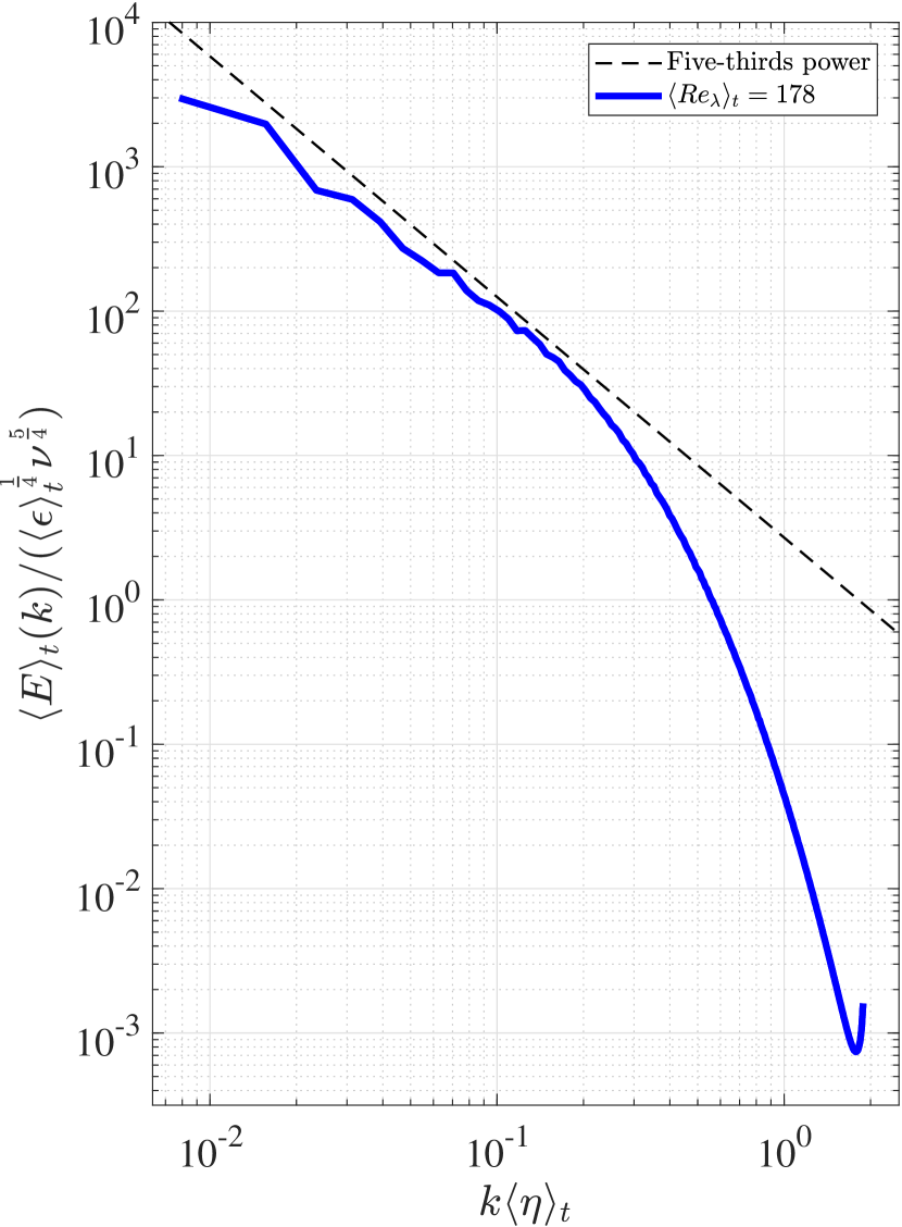
Figure 1: Time-average 3D energy spectrum of forced periodic turbulence. The dashed line indicates the 5/353-5/3 slope for reference.

The forcing method employed here is a negative damping forcing (see e.g. McComb et al., 2015; Linkmann & Morozov, 2015):

𝒇~(𝒌,t)~𝒇𝒌𝑡\displaystyle\tilde{\bm{f}}(\bm{k},t) =\displaystyle= (ϵW/2Kf)𝒖~(𝒌,t),for   0<|𝒌|<kf,subscriptitalic-ϵ𝑊2subscript𝐾𝑓~𝒖𝒌𝑡for   0𝒌subscript𝑘𝑓\displaystyle(\epsilon_{W}/2K_{f})\tilde{\bm{u}}(\bm{k},t),\>\>\>\>\>\>{\rm for}\>\>\>0<|\bm{k}|<k_{f}, (6)
=\displaystyle= 0,otherwise,0otherwise\displaystyle 0,\>\>\>\>\>\>\>\>\>\>\>\>\>\>\>\>\>\>\>\>\>\>\>\>\>\>\>\>\>\>\>\>\>\>\>\>\>\>\>\>\>\>\>{\rm otherwise}\>,

where 𝒇~(𝒌,t)~𝒇𝒌𝑡\tilde{\bm{f}}(\bm{k},t) and 𝒖~(𝒌,t)~𝒖𝒌𝑡\tilde{\bm{u}}(\bm{k},t) are the Fourier coefficients of 𝒇(𝒙,t)𝒇𝒙𝑡{\bm{f}}(\bm{x},t) and 𝒖(𝒙,t)𝒖𝒙𝑡{\bm{u}}(\bm{x},t) respectively, ϵWsubscriptitalic-ϵ𝑊\epsilon_{W} is the energy input rate per unit mass, kfsubscript𝑘𝑓k_{f} is the cutoff wavenumber, and Kfsubscript𝐾𝑓K_{f} is the total kinetic energy per unit mass contained in the forcing band 0<|𝒌|<kf0𝒌subscript𝑘𝑓0<|\bm{k}|<k_{f}. (We have also tried various other forcing methods without significant changes to our results all of which involve an average over two-point orientations as explained in the penultimate paragraph of this section and are therefore insensitive to any potential anisotropies introduced by forcing.) In our simulations, we set ϵW=0.1subscriptitalic-ϵ𝑊0.1\epsilon_{W}=0.1 and kf=2.5subscript𝑘𝑓2.5k_{f}=2.5. While ϵWsubscriptitalic-ϵ𝑊\epsilon_{W} is set constant in time, the total kinetic energy per unit mass K(t)𝐾𝑡K(t) and the total energy dissipation per unit mass ϵ(t)italic-ϵ𝑡\epsilon(t) fluctuate around constant values. We run two simulations and therefore use two mesh sizes, 1283superscript1283128^{3} and 5123superscript5123512^{3}, with respective kinematic viscosities ν=0.003𝜈0.003\nu=0.003 and 0.000720.000720.00072. Using these parameters, the simulations are run for about 82 and 35 eddy turnover times Lt/23Ktsubscriptdelimited-⟨⟩𝐿𝑡23subscriptdelimited-⟨⟩𝐾𝑡\langle L\rangle_{t}/\sqrt{{2\over 3}\langle K\rangle_{t}} respectively, where L𝐿L is the integral length-scale calculated from the 3D energy spectrum E(k,t)𝐸𝑘𝑡E(k,t), i.e. L(t)=3π40k1E(k,t)𝑑k/K(t)𝐿𝑡3𝜋4superscriptsubscript0superscript𝑘1𝐸𝑘𝑡differential-d𝑘𝐾𝑡L(t)={3\pi\over 4}\int_{0}^{\infty}k^{-1}E(k,t)dk/K(t). Throughout this work, suitably converged time-averages .t\langle.\rangle_{t} are calculated over 30 eddy turnover times for the 1283superscript1283128^{3} simulation and over 8.63 eddy turnover times for the 5123superscript5123512^{3} simulation, i.e. from t=25Lt/23Kt𝑡25subscriptdelimited-⟨⟩𝐿𝑡23subscriptdelimited-⟨⟩𝐾𝑡t=25\langle L\rangle_{t}/\sqrt{{2\over 3}\langle K\rangle_{t}} to t=55Lt/23Kt𝑡55subscriptdelimited-⟨⟩𝐿𝑡23subscriptdelimited-⟨⟩𝐾𝑡t=55\langle L\rangle_{t}/\sqrt{{2\over 3}\langle K\rangle_{t}} for 1283superscript1283128^{3} and from t=8.86Lt/23Kt𝑡8.86subscriptdelimited-⟨⟩𝐿𝑡23subscriptdelimited-⟨⟩𝐾𝑡t=8.86\langle L\rangle_{t}/\sqrt{{2\over 3}\langle K\rangle_{t}} to t=17.49Lt/23Kt𝑡17.49subscriptdelimited-⟨⟩𝐿𝑡23subscriptdelimited-⟨⟩𝐾𝑡t=17.49\langle L\rangle_{t}/\sqrt{{2\over 3}\langle K\rangle_{t}} for 5123superscript5123512^{3}. The time-averaged Taylor length-scale Reynolds number (based on the Taylor length λ=10νK/ϵ𝜆10𝜈𝐾italic-ϵ\lambda=\sqrt{10\nu K/\epsilon}) is Reλt=80.9subscriptdelimited-⟨⟩𝑅subscript𝑒𝜆𝑡80.9\langle Re_{\lambda}\rangle_{t}=80.9 and Reλt=178subscriptdelimited-⟨⟩𝑅subscript𝑒𝜆𝑡178\langle Re_{\lambda}\rangle_{t}=178 respectively. The average spatial resolution kmaxηtsubscript𝑘𝑚𝑎𝑥subscriptdelimited-⟨⟩𝜂𝑡k_{max}\langle\eta\rangle_{t} equals 1.371.371.37 for 1283superscript1283128^{3} and 1.891.891.89 for 5123superscript5123512^{3} with respective standard deviations 0.01890.01890.0189 and 0.04260.04260.0426, where η𝜂\eta is the Kolmogorov length. The time-average integral length-scale is related to kfsubscript𝑘𝑓k_{f} by 2π/kf=2.28Lt2𝜋subscript𝑘𝑓2.28subscriptdelimited-⟨⟩𝐿𝑡2\pi/k_{f}=2.28\langle L\rangle_{t} and 2π/kf=2.35Lt2𝜋subscript𝑘𝑓2.35subscriptdelimited-⟨⟩𝐿𝑡2\pi/k_{f}=2.35\langle L\rangle_{t} respectively and the standard deviations of λ𝜆\lambda and L𝐿L are 3.4% of λtsubscriptdelimited-⟨⟩𝜆𝑡\langle\lambda\rangle_{t} and 5.9% of Ltsubscriptdelimited-⟨⟩𝐿𝑡\langle L\rangle_{t} in the 1283superscript1283128^{3} case and 5.2% of λtsubscriptdelimited-⟨⟩𝜆𝑡\langle\lambda\rangle_{t} and 7.8% of Ltsubscriptdelimited-⟨⟩𝐿𝑡\langle L\rangle_{t} in the 5123superscript5123512^{3} case. In Fig. 1 the 3D energy spectrum is plotted for the 5123superscript5123512^{3} case.

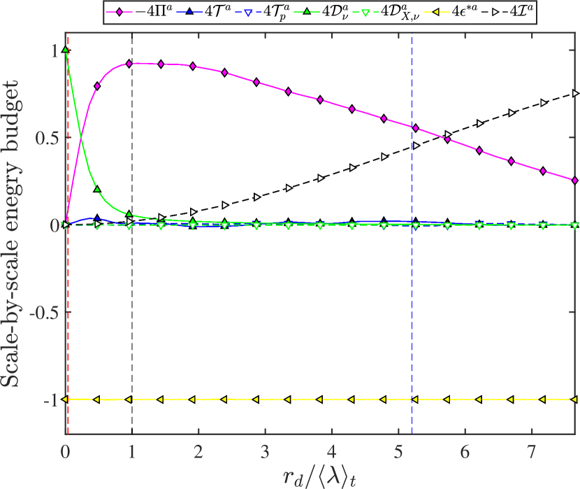
We now use our DNS to illustrate the average scale-by-scale energy budget (2). As this budget holds for arbitrary separation vector 𝒓𝒓{\bm{r}}, we calculate surface averages over spheres of diameter rdsubscript𝑟𝑑r_{d} in 𝒓𝒓\bm{r}-space and define Qa(rd)(πrd2)1|𝒓|=rdQ(𝒓)d𝒓superscript𝑄𝑎subscript𝑟𝑑superscript𝜋superscriptsubscript𝑟𝑑21subscripttriple-integral𝒓subscript𝑟𝑑𝑄𝒓differential-d𝒓Q^{a}(r_{d})\equiv(\pi r_{d}^{2})^{-1}\iiint\limits_{|\bm{r}|=r_{d}}Q(\bm{r}){\rm d}\bm{r} for any term Q𝑄Q in (1). In figure 2 we plot all the spatio-temporal average terms Qa(rd)delimited-⟨⟩superscript𝑄𝑎subscript𝑟𝑑\langle Q^{a}\rangle(r_{d}) normalised by 4ϵadelimited-⟨⟩4superscriptitalic-ϵabsent𝑎\langle 4\epsilon^{*a}\rangle as functions of rd/λtsubscript𝑟𝑑subscriptdelimited-⟨⟩𝜆𝑡r_{d}/\langle\lambda\rangle_{t}, where λtsubscriptdelimited-⟨⟩𝜆𝑡\langle\lambda\rangle_{t} is the time-average Taylor microscale. The only non-zero terms are indeed those present in the average balance (2). We recover the kinematic constraints (i) 𝒟νa=ϵadelimited-⟨⟩superscriptsubscript𝒟𝜈𝑎delimited-⟨⟩superscriptitalic-ϵabsent𝑎\langle\mathcal{D}_{\nu}^{a}\rangle=\langle\epsilon^{*a}\rangle at rd=0subscript𝑟𝑑0r_{d}=0 and (ii) that 𝒟νadelimited-⟨⟩superscriptsubscript𝒟𝜈𝑎\langle\mathcal{D}_{\nu}^{a}\rangle is negligible compared to ϵadelimited-⟨⟩superscriptitalic-ϵabsent𝑎\langle\epsilon^{*a}\rangle for rdsubscript𝑟𝑑r_{d} smaller than the Taylor microscale (Valente & Vassilicos, 2015). At scales rdsubscript𝑟𝑑r_{d} larger than the Taylor microscale, Πaϵa+adelimited-⟨⟩superscriptΠ𝑎delimited-⟨⟩superscriptitalic-ϵabsent𝑎delimited-⟨⟩superscript𝑎\langle\Pi^{a}\rangle\approx-\langle\epsilon^{*a}\rangle+\langle\mathcal{I}^{a}\rangle, see (2), and one can see from figure 2 that the direct influence of the large-scale energy input rate diminishes as rdsubscript𝑟𝑑r_{d} decreases below the integral length-scale and towards the Taylor micro-scale. One might imagine that, as the Reynolds number increases above the values in the present DNS, the direct influence of the large-scale forcing might disappear in much of the inertial range of scales between λtsubscriptdelimited-⟨⟩𝜆𝑡\langle\lambda\rangle_{t} and Ltsubscriptdelimited-⟨⟩𝐿𝑡\langle L\rangle_{t} leading to Πaϵadelimited-⟨⟩superscriptΠ𝑎delimited-⟨⟩superscriptitalic-ϵabsent𝑎\langle\Pi^{a}\rangle\approx-\langle\epsilon^{*a}\rangle in much of that range. This approximate equality encapsulates the Kolmogorov equilibrium cascade. This is an average cascade where the turbulent energy cascades from large to small inertial scales at constant rate approximately equal to the dissipation rate.
Refer to caption
Figure 2: Average scale-by-scale energy budget for statistically stationary periodic turbulence (Reλt=178subscriptdelimited-⟨⟩𝑅subscript𝑒𝜆𝑡178\langle Re_{\lambda}\rangle_{t}=178): plots of Qa(rd)delimited-⟨⟩superscript𝑄𝑎subscript𝑟𝑑\langle Q^{a}\rangle(r_{d}) normalised by 4ϵadelimited-⟨⟩4superscriptitalic-ϵabsent𝑎\langle 4\epsilon^{*a}\rangle versus rd/λtsubscript𝑟𝑑subscriptdelimited-⟨⟩𝜆𝑡r_{d}/\langle\lambda\rangle_{t} for the terms, generically referred to as Q𝑄Q in this caption, in (1). The actual list of these terms is at the top of the plot. Vertical red, black, blue dashed lines denote the Kolmogorov scale ηtsubscriptdelimited-⟨⟩𝜂𝑡\langle\eta\rangle_{t}, the Taylor-micro scale λtsubscriptdelimited-⟨⟩𝜆𝑡\langle\lambda\rangle_{t}, and the integral scale Ltsubscriptdelimited-⟨⟩𝐿𝑡\langle L\rangle_{t}, respectively. Similar results (not plotted here) are obtained for Reλt=80.9subscriptdelimited-⟨⟩𝑅subscript𝑒𝜆𝑡80.9\langle Re_{\lambda}\rangle_{t}=80.9 except that the maximum value of 4Πa4superscriptΠ𝑎-4\Pi^{a} is smaller and the decrease of 4Πa4superscriptΠ𝑎-4\Pi^{a} from rd=λtsubscript𝑟𝑑subscriptdelimited-⟨⟩𝜆𝑡r_{d}=\langle\lambda\rangle_{t} to rd=Ltsubscript𝑟𝑑subscriptdelimited-⟨⟩𝐿𝑡r_{d}=\langle L\rangle_{t} is steeper because this range of scales is also smaller (Lt/λt2.7subscriptdelimited-⟨⟩𝐿𝑡subscriptdelimited-⟨⟩𝜆𝑡2.7\langle L\rangle_{t}/\langle\lambda\rangle_{t}\approx 2.7 for Reλt=80.9subscriptdelimited-⟨⟩𝑅subscript𝑒𝜆𝑡80.9\langle Re_{\lambda}\rangle_{t}=80.9).

(a)

Refer to caption

(b)

Refer to caption
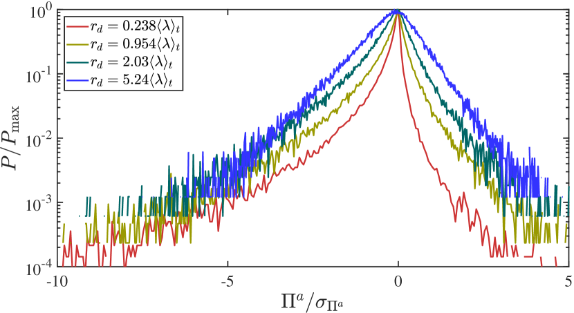
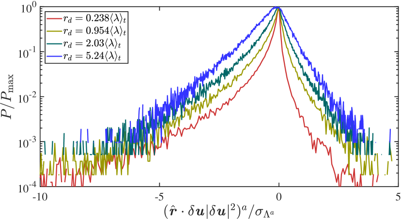
Figure 3: (a) PDFs of ΠasuperscriptΠ𝑎\Pi^{a} obtained by sampling through both space and time and plotted versus Πa/σΠasuperscriptΠ𝑎subscript𝜎superscriptΠ𝑎\Pi^{a}/\sigma_{\Pi^{a}} where Πa(rd)(πrd2)1|𝒓|=rdΠ(𝒓)d𝒓superscriptΠ𝑎subscript𝑟𝑑superscript𝜋superscriptsubscript𝑟𝑑21subscripttriple-integral𝒓subscript𝑟𝑑Π𝒓differential-d𝒓\Pi^{a}(r_{d})\equiv(\pi r_{d}^{2})^{-1}\iiint\limits_{|\bm{r}|=r_{d}}\Pi(\bm{r}){\rm d}\bm{r} and σΠasubscript𝜎superscriptΠ𝑎\sigma_{\Pi^{a}} is the standard deviation of ΠasuperscriptΠ𝑎\Pi^{a}. (b) PDFs of (𝒓^δ𝒖|δ𝒖|2)a(πrd2)1|𝒓|=rd𝒓^δ𝒖|δ𝒖|2d𝒓superscriptbold-^𝒓𝛿𝒖superscript𝛿𝒖2𝑎superscript𝜋superscriptsubscript𝑟𝑑21subscripttriple-integral𝒓subscript𝑟𝑑bold-^𝒓𝛿𝒖superscript𝛿𝒖2differential-d𝒓(\bm{\hat{r}}\cdot\delta\bm{u}|\delta\bm{u}|^{2})^{a}\equiv(\pi r_{d}^{2})^{-1}\iiint\limits_{|\bm{r}|=r_{d}}\bm{\hat{r}}\cdot\delta\bm{u}|\delta\bm{u}|^{2}{\rm d}\bm{r} obtained by sampling through both space and time and plotted versus (𝒓^δ𝒖|δ𝒖|2)a/σΛasuperscriptbold-^𝒓𝛿𝒖superscript𝛿𝒖2𝑎subscript𝜎superscriptΛ𝑎(\bm{\hat{r}}\cdot\delta\bm{u}|\delta\bm{u}|^{2})^{a}/\sigma_{\Lambda^{a}} where σΛasubscript𝜎superscriptΛ𝑎\sigma_{\Lambda^{a}} is the standard deviation of (𝒓^δ𝒖|δ𝒖|2)asuperscriptbold-^𝒓𝛿𝒖superscript𝛿𝒖2𝑎(\bm{\hat{r}}\cdot\delta\bm{u}|\delta\bm{u}|^{2})^{a}. Reλt=178subscriptdelimited-⟨⟩𝑅subscript𝑒𝜆𝑡178\langle Re_{\lambda}\rangle_{t}=178 but the plots are similar for Reλt=80.9subscriptdelimited-⟨⟩𝑅subscript𝑒𝜆𝑡80.9\langle Re_{\lambda}\rangle_{t}=80.9. Red, yellow, green and blue lines correspond to rd=0.238λtsubscript𝑟𝑑0.238subscriptdelimited-⟨⟩𝜆𝑡r_{d}=0.238\langle\lambda\rangle_{t}, 0.954λt0.954subscriptdelimited-⟨⟩𝜆𝑡0.954\langle\lambda\rangle_{t}, 2.03λt2.03subscriptdelimited-⟨⟩𝜆𝑡2.03\langle\lambda\rangle_{t} and 5.24λt5.24subscriptdelimited-⟨⟩𝜆𝑡5.24\langle\lambda\rangle_{t}, where λ𝜆\lambda is the Taylor-micro scale and tsubscriptdelimited-⟨⟩𝑡\langle\cdot\rangle_{t} denotes a long-term average.

This average picture is punctuated by the known fact (Piomelli et al., 1991; Domaradzki et al., 1993; Cerutti & Meneveau, 1998; Aoyama et al., 2005; Goto, 2008; Ishihara et al., 2009) that the interscale energy transfer rate ΠΠ\Pi is highly intermittent, as indeed confirmed by our DNS. In figure 3 we plot the PDFs of ΠasuperscriptΠ𝑎\Pi^{a} and of (𝒓^δ𝒖|δ𝒖|2)asuperscriptbold-^𝒓𝛿𝒖superscript𝛿𝒖2𝑎(\bm{\hat{r}}\cdot\delta\bm{u}|\delta\bm{u}|^{2})^{a} for two length-scales rdsubscript𝑟𝑑r_{d} in the approximately inertial range of our simulation, rd/λt2subscript𝑟𝑑subscriptdelimited-⟨⟩𝜆𝑡2r_{d}/\langle\lambda\rangle_{t}\approx 2 and 555, and two length-scales rdsubscript𝑟𝑑r_{d} in the dissipation range at and below λtsubscriptdelimited-⟨⟩𝜆𝑡\langle\lambda\rangle_{t}. Figure 3(a) is qualitatively similar to figure 6 in Ishihara et al. (2009) and, along with figure 3(b), reveals very clearly the highly intermittent and non-Gaussian nature of ΠasuperscriptΠ𝑎\Pi^{a} and (𝒓^δ𝒖|δ𝒖|2)asuperscriptbold-^𝒓𝛿𝒖superscript𝛿𝒖2𝑎(\bm{\hat{r}}\cdot\delta\bm{u}|\delta\bm{u}|^{2})^{a} given the very heavy tails of their PDFs. The equality between the volume integral |𝒓|rd4Π(𝑿,𝒓,t)𝑑𝒓subscripttriple-integral𝒓subscript𝑟𝑑4Π𝑿𝒓𝑡differential-d𝒓\iiint\limits_{|\bm{r}|\leq r_{d}}4\Pi(\bm{X},\bm{r},t)d{\bm{r}} and the surface integral |𝒓|=rdδ𝒖𝒓^|δ𝒖|2𝑑𝒓subscripttriple-integral𝒓subscript𝑟𝑑𝛿𝒖^𝒓superscript𝛿𝒖2differential-d𝒓\iiint\limits_{|\bm{r}|=r_{d}}{\delta{\bm{u}}}\cdot\hat{\bm{r}}|{\delta{\bm{u}}}|^{2}d{\bm{r}} implies that compression events where δ𝒖𝒓^<0𝛿𝒖^𝒓0\delta{\bm{u}}\cdot\hat{\bm{r}}<0 contribute to the forward cascade from large to small scales whereas stretching events where δ𝒖𝒓^>0𝛿𝒖^𝒓0\delta{\bm{u}}\cdot\hat{\bm{r}}>0 contribute to backscatter, i.e. from small to large scales. We also found a significant positive correlation between ΠasuperscriptΠ𝑎\Pi^{a} and (𝒓^δ𝒖|δ𝒖|2)asuperscriptbold-^𝒓𝛿𝒖superscript𝛿𝒖2𝑎(\bm{\hat{r}}\cdot\delta\bm{u}|\delta\bm{u}|^{2})^{a}; their correlation coefficient (calculated by averaging over both space and time) is close to 1 near rd=0subscript𝑟𝑑0r_{d}=0 and decreases gently with increasing rdsubscript𝑟𝑑r_{d} reaching values approximately equal to 0.9 at rdλtsubscript𝑟𝑑subscriptdelimited-⟨⟩𝜆𝑡r_{d}\approx\langle\lambda\rangle_{t} and 0.6 at rdLtsubscript𝑟𝑑subscriptdelimited-⟨⟩𝐿𝑡r_{d}\approx\langle L\rangle_{t} (for Reλt=178subscriptdelimited-⟨⟩𝑅subscript𝑒𝜆𝑡178\langle Re_{\lambda}\rangle_{t}=178). Hence, positive/negative values of ΠasuperscriptΠ𝑎\Pi^{a} correlate with forward/backscatter cascade events and figure 3 confirms that backscatter and extreme forward cascade events exist with much higher probability than for a normal distribution. In fact, these rare but powerful forward and inverse cascade events are so very significant that 50% of the average values Πadelimited-⟨⟩superscriptΠ𝑎\langle\Pi^{a}\rangle and (𝒓^δ𝒖|δ𝒖|2)adelimited-⟨⟩superscriptbold-^𝒓𝛿𝒖superscript𝛿𝒖2𝑎\langle(\bm{\hat{r}}\cdot\delta\bm{u}|\delta\bm{u}|^{2})^{a}\rangle are contributed by events whose probabilities are lower than 0.0157PmaxΠ0.0157subscriptsuperscript𝑃Π𝑚𝑎𝑥0.0157P^{\Pi}_{max} and 0.0145PmaxΛ0.0145subscriptsuperscript𝑃Λ𝑚𝑎𝑥0.0145P^{\Lambda}_{max} respectively at rd=0.977λtsubscript𝑟𝑑0.977subscriptdelimited-⟨⟩𝜆𝑡r_{d}=0.977\langle\lambda\rangle_{t}; lower than 0.0350PmaxΠ0.0350subscriptsuperscript𝑃Π𝑚𝑎𝑥0.0350P^{\Pi}_{max} and 0.0299PmaxΛ0.0299subscriptsuperscript𝑃Λ𝑚𝑎𝑥0.0299P^{\Lambda}_{max} respectively at rd=2.03λtsubscript𝑟𝑑2.03subscriptdelimited-⟨⟩𝜆𝑡r_{d}=2.03\langle\lambda\rangle_{t}; and lower than 0.0801PmaxΠ0.0801subscriptsuperscript𝑃Π𝑚𝑎𝑥0.0801P^{\Pi}_{max} and 0.0738PmaxΛ0.0738subscriptsuperscript𝑃Λ𝑚𝑎𝑥0.0738P^{\Lambda}_{max} respectively at rd=5.24λtsubscript𝑟𝑑5.24subscriptdelimited-⟨⟩𝜆𝑡r_{d}=5.24\langle\lambda\rangle_{t} which is close to Ltsubscriptdelimited-⟨⟩𝐿𝑡\langle L\rangle_{t}. These probabilities are given for Reλt=178subscriptdelimited-⟨⟩𝑅subscript𝑒𝜆𝑡178\langle Re_{\lambda}\rangle_{t}=178 and are even lower than for Reλt=80.9subscriptdelimited-⟨⟩𝑅subscript𝑒𝜆𝑡80.9\langle Re_{\lambda}\rangle_{t}=80.9 (e.g. for Reλt=80.9subscriptdelimited-⟨⟩𝑅subscript𝑒𝜆𝑡80.9\langle Re_{\lambda}\rangle_{t}=80.9, 50% of the average value Πadelimited-⟨⟩superscriptΠ𝑎\langle\Pi^{a}\rangle is contributed by events whose probabilities are lower than 0.0235PmaxΠ0.0235subscriptsuperscript𝑃Π𝑚𝑎𝑥0.0235P^{\Pi}_{max} if rd=0.977λtsubscript𝑟𝑑0.977subscriptdelimited-⟨⟩𝜆𝑡r_{d}=0.977\langle\lambda\rangle_{t} and lower than 0.0467PmaxΠ0.0467subscriptsuperscript𝑃Π𝑚𝑎𝑥0.0467P^{\Pi}_{max} if rd=1.95λtsubscript𝑟𝑑1.95subscriptdelimited-⟨⟩𝜆𝑡r_{d}=1.95\langle\lambda\rangle_{t}). PmaxΠsubscriptsuperscript𝑃Π𝑚𝑎𝑥P^{\Pi}_{max} and PmaxΛsubscriptsuperscript𝑃Λ𝑚𝑎𝑥P^{\Lambda}_{max} are the probabilities of the most likely events which are, respectively, Πa=0superscriptΠ𝑎0\Pi^{a}=0 and (𝒓^δ𝒖|δ𝒖|2)a=0superscriptbold-^𝒓𝛿𝒖superscript𝛿𝒖2𝑎0(\bm{\hat{r}}\cdot\delta\bm{u}|\delta\bm{u}|^{2})^{a}=0, i.e. no interscale energy transfer whatsoever. The asymmetry of the PDFs in figure 3 ensures that Πadelimited-⟨⟩superscriptΠ𝑎\langle\Pi^{a}\rangle is negative on average and that the average picture is therefore one of forward interscale energy transfer. However, this average picture requires extreme events, both forward and backward, to fully emerge. As mentioned in the introduction, the extreme intermittency of ΠasuperscriptΠ𝑎\Pi^{a} raises the question of the fluctuations of all the other terms in the KHMH equation, particularly those which average out to zero and could therefore be thought of as unimportant. Having presented and validated our DNS and KHMH approach in this section, we now move to the new results of this paper.

(a)
Refer to caption

(b)

Refer to caption

(c)

Refer to caption

(d)

Refer to caption
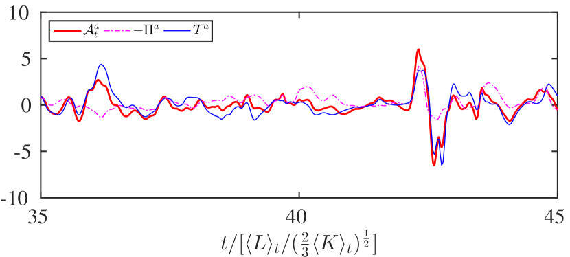
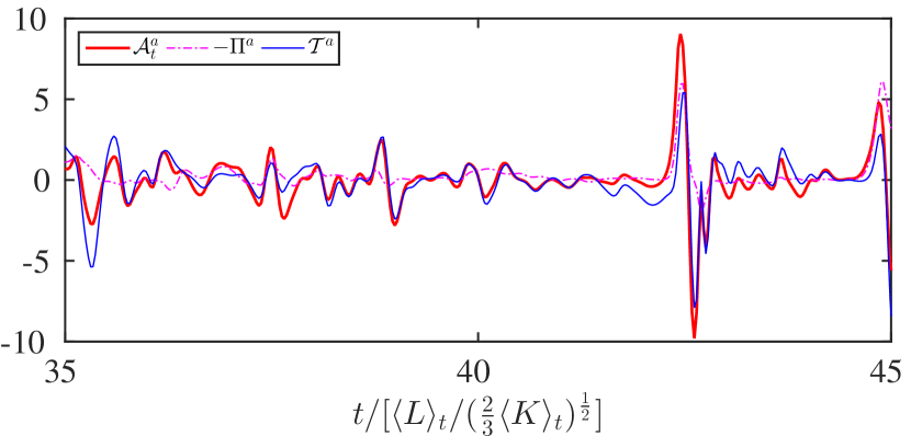
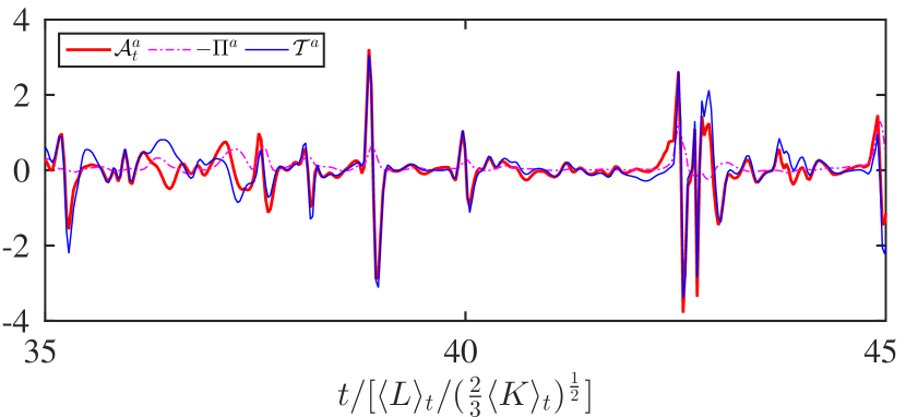
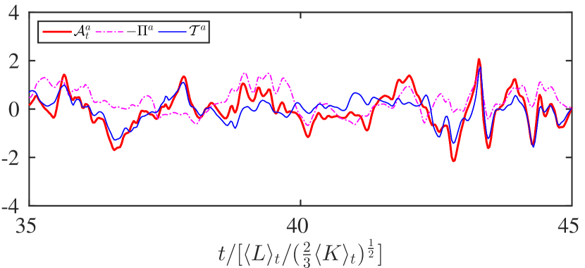
Figure 4: Time evolutions of 𝒜tasuperscriptsubscript𝒜𝑡𝑎\mathcal{A}_{t}^{a}, ΠasuperscriptΠ𝑎-\Pi^{a} and 𝒯asuperscript𝒯𝑎\mathcal{T}^{a} at a random location 𝑿𝑿{\bm{X}} and four different scales. Reλt=80.9subscriptdelimited-⟨⟩𝑅subscript𝑒𝜆𝑡80.9\langle Re_{\lambda}\rangle_{t}=80.9. Red, magenta, blue lines represent 𝒜tasuperscriptsubscript𝒜𝑡𝑎\mathcal{A}_{t}^{a}, ΠasuperscriptΠ𝑎-\Pi^{a}, 𝒯asuperscript𝒯𝑎\mathcal{T}^{a}, respectively. (a) rd=3.91λtsubscript𝑟𝑑3.91subscriptdelimited-⟨⟩𝜆𝑡r_{d}=3.91\langle\lambda\rangle_{t}, (b) 1.95λt1.95subscriptdelimited-⟨⟩𝜆𝑡1.95\langle\lambda\rangle_{t}, (c) 0.977λt0.977subscriptdelimited-⟨⟩𝜆𝑡0.977\langle\lambda\rangle_{t}, (d) 0.244λt0.244subscriptdelimited-⟨⟩𝜆𝑡0.244\langle\lambda\rangle_{t}.

4 Fluctuating and correlated interscale and interspace energy transfer dynamics

In figure 4 we plot representative examples of time evolutions of some orientation-averaged KHMH terms at a randomly selected location 𝑿𝑿{\bm{X}}, specifically 𝒜tasuperscriptsubscript𝒜𝑡𝑎\mathcal{A}_{t}^{a}, 𝒯asuperscript𝒯𝑎\mathcal{T}^{a} and ΠasuperscriptΠ𝑎-\Pi^{a}, for four different values of rdsubscript𝑟𝑑r_{d} (rd/λt=3.91,1.95,0.977,0.224subscript𝑟𝑑subscriptdelimited-⟨⟩𝜆𝑡3.911.950.9770.224r_{d}/\langle\lambda\rangle_{t}=3.91,1.95,0.977,0.224). We chose to plot only a few of the zero-average KHMH terms for clarity of exposition and we plot them alongside ΠasuperscriptΠ𝑎-\Pi^{a} to compare fluctuations. We also chose to show plots in figure 4 which have been obtained for Reλt=80.9subscriptdelimited-⟨⟩𝑅subscript𝑒𝜆𝑡80.9\langle Re_{\lambda}\rangle_{t}=80.9 but very similar plots are also obtained for Reλt=178subscriptdelimited-⟨⟩𝑅subscript𝑒𝜆𝑡178\langle Re_{\lambda}\rangle_{t}=178. Plots of the same terms at a randomly selected time t𝑡t but as functions of X1subscript𝑋1X_{1}, X2subscript𝑋2X_{2} or X3subscript𝑋3X_{3} rather than as functions of t𝑡t for a randomly selected 𝑿=(X1,X2,X3)𝑿subscript𝑋1subscript𝑋2subscript𝑋3{\bm{X}}=(X_{1},X_{2},X_{3}), look similar to those in figure 4 and lead to the same observations.

At the largest rdsubscript𝑟𝑑r_{d} in figure 4 (which is 1.47 Ltsubscriptdelimited-⟨⟩𝐿𝑡\langle L\rangle_{t}) the fluctuations of all three quantities are comparable and one can even detect a correlation between them (figure 4(a)). With decreasing rdsubscript𝑟𝑑r_{d}, all three signals become increasingly intermittent; all three PDFs exhibit increasingly heavy tails (not all shown here for economy of space) with decreasing rdsubscript𝑟𝑑r_{d} as in figure 3, except that the PDFs of 𝒜tasuperscriptsubscript𝒜𝑡𝑎\mathcal{A}_{t}^{a} and 𝒯asuperscript𝒯𝑎\mathcal{T}^{a} are symmetric whereas the PDF of ΠasuperscriptΠ𝑎-\Pi^{a} is skewed (see figure 3). The fluctuations of 𝒜tasuperscriptsubscript𝒜𝑡𝑎\mathcal{A}_{t}^{a} and 𝒯asuperscript𝒯𝑎\mathcal{T}^{a} grow in magnitude with decreasing rdsubscript𝑟𝑑r_{d} whereas those of ΠasuperscriptΠ𝑎-\Pi^{a} do not so significantly. Furthermore, the correlation between 𝒜tasuperscriptsubscript𝒜𝑡𝑎\mathcal{A}_{t}^{a} and 𝒯asuperscript𝒯𝑎\mathcal{T}^{a} strengthens whereas the correlation of ΠasuperscriptΠ𝑎-\Pi^{a} with the other two signals weakens.

(a)
Refer to caption

(b)

Refer to caption
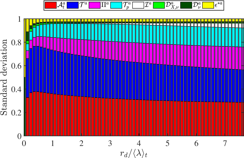
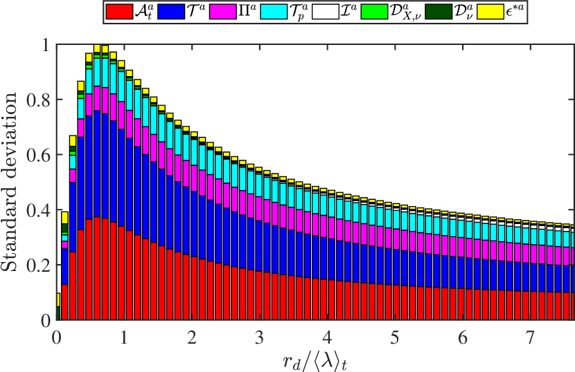
Figure 5: Stacked column chart of standard deviations of KHMH terms as a function of rd/λtsubscript𝑟𝑑subscriptdelimited-⟨⟩𝜆𝑡r_{d}/\langle\lambda\rangle_{t}. Vertical axis is normalized by (a) the total height of the largest stacked column and (b) the total height of each stacked column. Reλt=178subscriptdelimited-⟨⟩𝑅subscript𝑒𝜆𝑡178\langle Re_{\lambda}\rangle_{t}=178 but similar results are obtained for Reλt=80.9subscriptdelimited-⟨⟩𝑅subscript𝑒𝜆𝑡80.9\langle Re_{\lambda}\rangle_{t}=80.9.

(a1)

Refer to caption

(b1)

Refer to caption

(a2)

Refer to caption

(b2)

Refer to caption
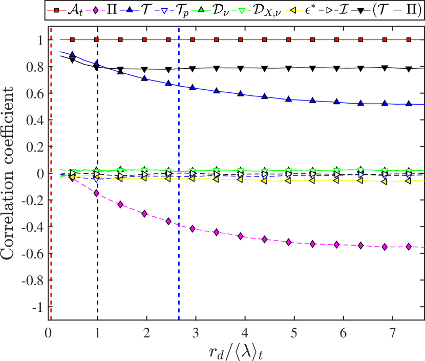
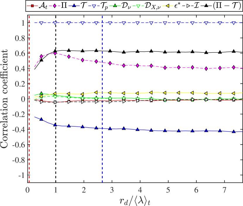
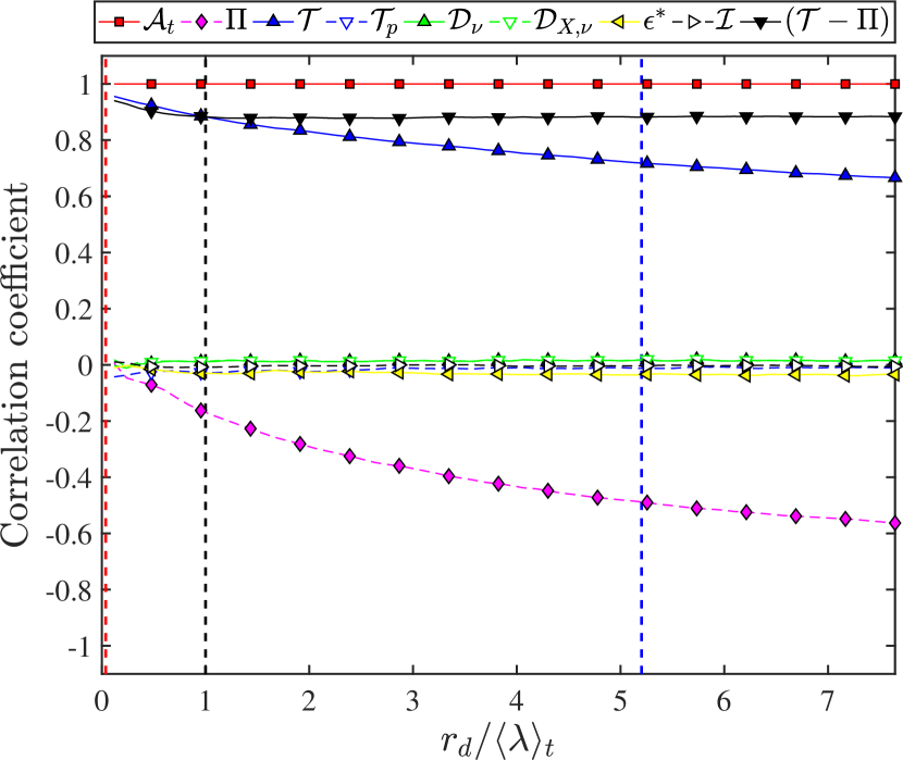
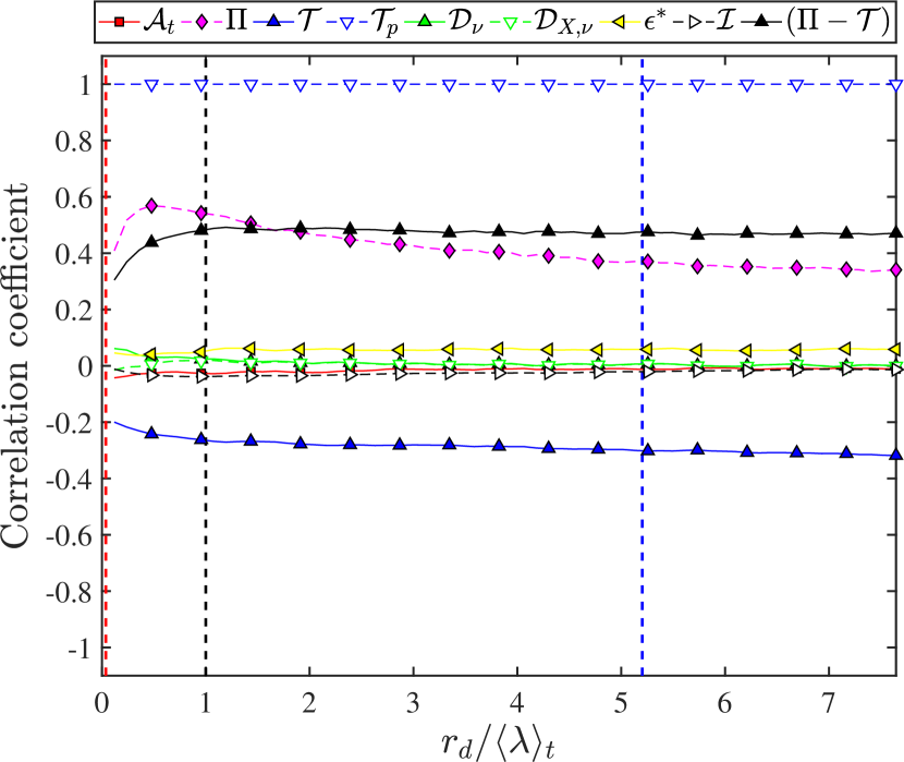
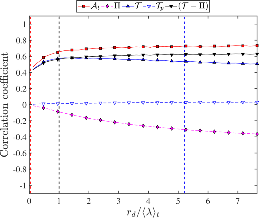
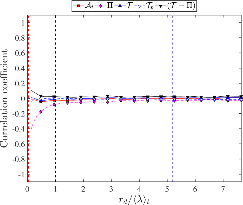
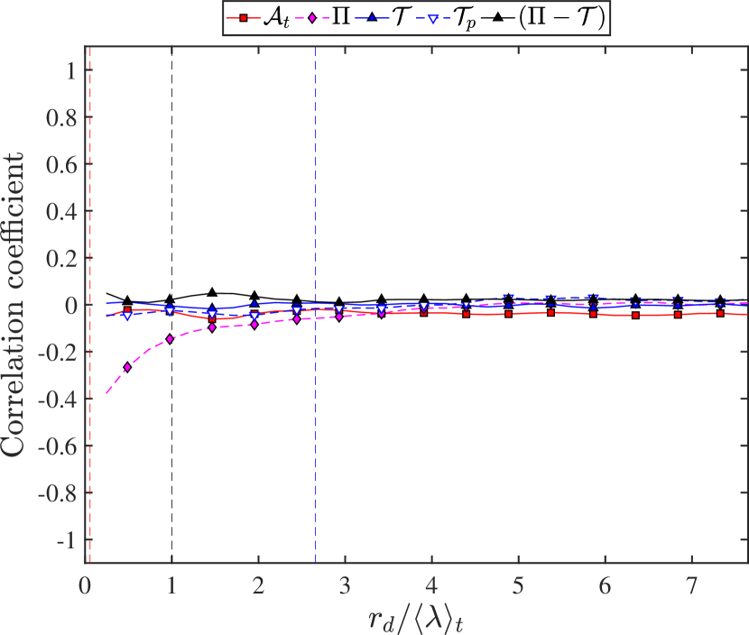
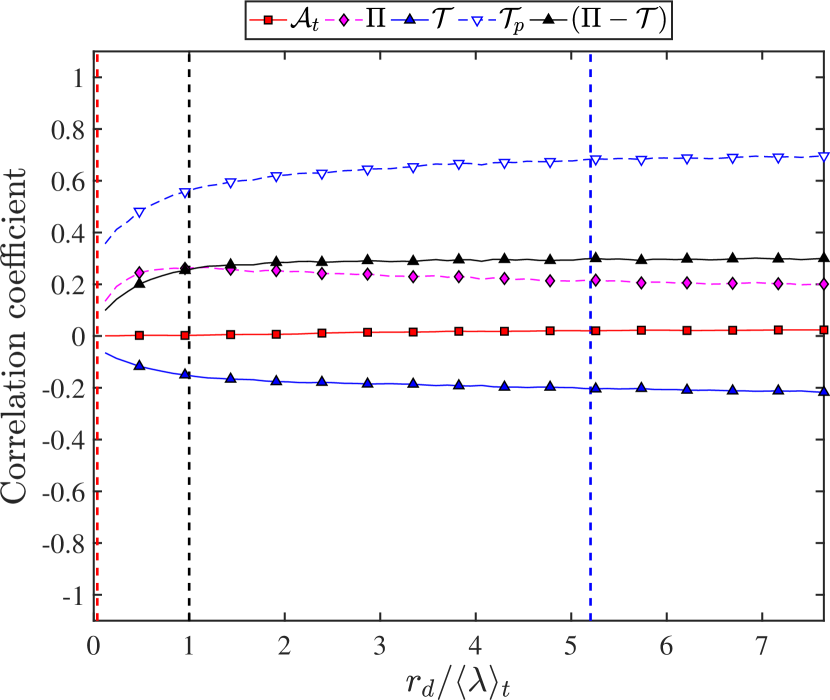
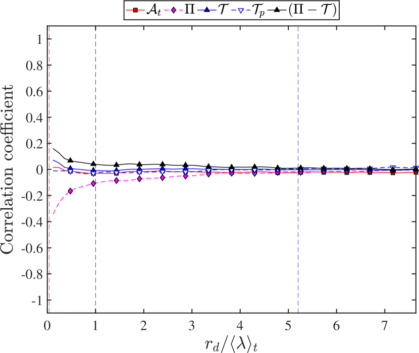
Figure 6: Correlation coefficients corr(Q1,Q2)𝑐𝑜𝑟𝑟subscript𝑄1subscript𝑄2corr(Q_{1},Q_{2}) (defined in the second paragraph of subsection 4.1) for the nine Q2subscript𝑄2Q_{2} terms indicated above the plots and (a1) Q1=𝒜tsubscript𝑄1subscript𝒜𝑡Q_{1}=\mathcal{A}_{t} and Reλt=80.9subscriptdelimited-⟨⟩𝑅subscript𝑒𝜆𝑡80.9\langle Re_{\lambda}\rangle_{t}=80.9, (a2) Q1=𝒜tsubscript𝑄1subscript𝒜𝑡Q_{1}=\mathcal{A}_{t} and Reλt=178subscriptdelimited-⟨⟩𝑅subscript𝑒𝜆𝑡178\langle Re_{\lambda}\rangle_{t}=178, (b1) Q1=𝒯psubscript𝑄1subscript𝒯𝑝Q_{1}=\mathcal{T}_{p} and Reλt=80.9subscriptdelimited-⟨⟩𝑅subscript𝑒𝜆𝑡80.9\langle Re_{\lambda}\rangle_{t}=80.9, (b2) Q1=𝒯psubscript𝑄1subscript𝒯𝑝Q_{1}=\mathcal{T}_{p} and Reλt=178subscriptdelimited-⟨⟩𝑅subscript𝑒𝜆𝑡178\langle Re_{\lambda}\rangle_{t}=178. These correlation coefficients are calculated by sampling over space 𝑿𝑿{\bm{X}}, time t𝑡t and orientations 𝒓^^𝒓\hat{\bm{r}} for a given rdsubscript𝑟𝑑r_{d} such that 𝒓=rd𝒓^𝒓subscript𝑟𝑑^𝒓{\bm{r}}=r_{d}\hat{\bm{r}}. They are plotted as functions rdsubscript𝑟𝑑r_{d} and normalised by λtsubscriptdelimited-⟨⟩𝜆𝑡\langle\lambda\rangle_{t}. The red, black and blue dashed vertical straight lines indicate the time-average Kolmogorov scale ηtsubscriptdelimited-⟨⟩𝜂𝑡\langle\eta\rangle_{t}, Taylor micro scale λtsubscriptdelimited-⟨⟩𝜆𝑡\langle\lambda\rangle_{t}, and integral scale Ltsubscriptdelimited-⟨⟩𝐿𝑡\langle L\rangle_{t}, respectively.

(a)

Refer to caption

(b)

Refer to caption
Figure 7: (a) Correlation coefficients corr(Q1,Q2)𝑐𝑜𝑟𝑟subscript𝑄1subscript𝑄2corr(Q_{1},Q_{2}) (defined in the second paragraph of subsection 4.1) for Q1=cosθsubscript𝑄1𝜃Q_{1}=\cos\theta and Q2=subscript𝑄2absentQ_{2}= 𝒜tsubscript𝒜𝑡\mathcal{A}_{t}, ΠΠ\Pi, 𝒯𝒯\mathcal{T}, 𝒯psubscript𝒯𝑝\mathcal{T}_{p} and 𝒯Π𝒯script-Π\mathcal{T}-\mathcal{\Pi}. (b) Correlation coefficients corr(Q1,Q2)𝑐𝑜𝑟𝑟subscript𝑄1subscript𝑄2corr(Q_{1},Q_{2}) for Q1=|δ𝒖||δt𝒖|subscript𝑄1𝛿𝒖𝛿𝑡𝒖Q_{1}=|\delta{\bm{u}}||\delta\frac{\partial}{\partial t}{\bm{u}}| and Q2=subscript𝑄2absentQ_{2}= 𝒜tsubscript𝒜𝑡\mathcal{A}_{t}, ΠΠ\Pi, 𝒯𝒯\mathcal{T}, 𝒯psubscript𝒯𝑝\mathcal{T}_{p} and 𝒯Π𝒯script-Π\mathcal{T}-\mathcal{\Pi}. The correlation coefficients in these two plots are calculated and plotted as explained in the caption of figure 6, and the red, black and blue dashed vertical straight lines are the same as in figure 6. Reλt=178subscriptdelimited-⟨⟩𝑅subscript𝑒𝜆𝑡178\langle Re_{\lambda}\rangle_{t}=178 but these plots are very similar for Reλt=80.9subscriptdelimited-⟨⟩𝑅subscript𝑒𝜆𝑡80.9\langle Re_{\lambda}\rangle_{t}=80.9.

(a)

Refer to caption

(b)

Refer to caption
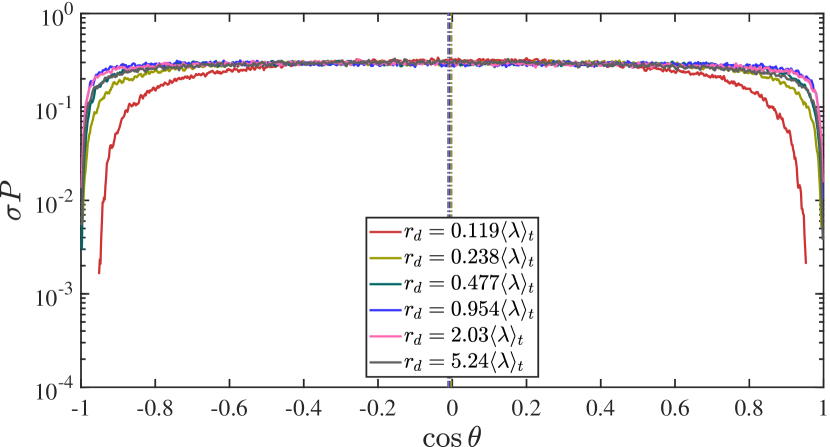
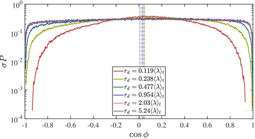
Figure 8: PDFs of cosines of angles obtained from sampling over 𝑿𝑿{\bm{X}}, t𝑡t and 𝒓^^𝒓\hat{\bm{r}} for a given rd=|𝒓|subscript𝑟𝑑𝒓r_{d}=|{\bm{r}}|. Different curves correspond to different values of rdsubscript𝑟𝑑r_{d} as shown in the insert. (a) PDFs of cosθ𝜃\cos\theta multiplied by the standard deviation of cosθ𝜃\cos\theta. The vertical line indicates the average cosθallsubscriptdelimited-⟨⟩𝜃𝑎𝑙𝑙\langle\cos\theta\rangle_{all} (average over 𝑿𝑿{\bm{X}}, t𝑡t and 𝒓^^𝒓\hat{\bm{r}}) which is effectively 00 for all rdsubscript𝑟𝑑r_{d}. (b) PDFs of cosϕitalic-ϕ\cos\phi multiplied by the standard deviation of cosϕitalic-ϕ\cos\phi. The vertical lines indicate the average cosϕallsubscriptdelimited-⟨⟩italic-ϕ𝑎𝑙𝑙\langle\cos\phi\rangle_{all} for different values of rdsubscript𝑟𝑑r_{d} from 0.119λt0.119subscriptdelimited-⟨⟩𝜆𝑡0.119\langle\lambda\rangle_{t} to 5.24λt5.24subscriptdelimited-⟨⟩𝜆𝑡5.24\langle\lambda\rangle_{t}. The average of cosϕitalic-ϕ\cos\phi is very close to 00 for rd5.24λtsubscript𝑟𝑑5.24subscriptdelimited-⟨⟩𝜆𝑡r_{d}\leq 5.24\langle\lambda\rangle_{t} (Ltabsentsubscriptdelimited-⟨⟩𝐿𝑡\approx\langle L\rangle_{t}); in the range below 5.24λt5.24subscriptdelimited-⟨⟩𝜆𝑡5.24\langle\lambda\rangle_{t}, it increases monotonically with decreasing rdsubscript𝑟𝑑r_{d} till it reaches 0.05absent0.05\approx 0.05 at rd=0.119λtsubscript𝑟𝑑0.119subscriptdelimited-⟨⟩𝜆𝑡r_{d}=0.119\langle\lambda\rangle_{t}. Reλt=178subscriptdelimited-⟨⟩𝑅subscript𝑒𝜆𝑡178\langle Re_{\lambda}\rangle_{t}=178 but these plots are very similar for Reλt=80.9subscriptdelimited-⟨⟩𝑅subscript𝑒𝜆𝑡80.9\langle Re_{\lambda}\rangle_{t}=80.9.

(a1)

Refer to caption

(b1)

Refer to caption

(a2)

Refer to caption

(b2)

Refer to caption
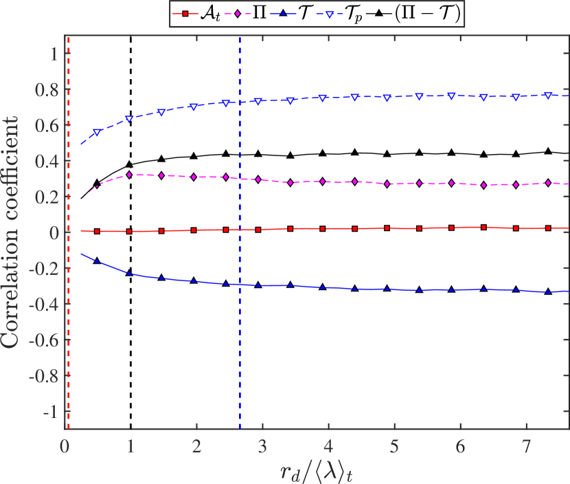
Figure 9: (a1-a2) Correlation coefficients corr(Q1,Q2)𝑐𝑜𝑟𝑟subscript𝑄1subscript𝑄2corr(Q_{1},Q_{2}) (defined in the second paragraph of subsection 4.1) for Q1=cosϕsubscript𝑄1italic-ϕQ_{1}=\cos\phi and Q2=subscript𝑄2absentQ_{2}= 𝒜tsubscript𝒜𝑡\mathcal{A}_{t}, ΠΠ\Pi, 𝒯𝒯\mathcal{T}, 𝒯psubscript𝒯𝑝\mathcal{T}_{p} and Π𝒯script-Π𝒯\mathcal{\Pi}-\mathcal{T}: (a1) for Reλt=80.9subscriptdelimited-⟨⟩𝑅subscript𝑒𝜆𝑡80.9\langle Re_{\lambda}\rangle_{t}=80.9, (a2) for Reλt=178subscriptdelimited-⟨⟩𝑅subscript𝑒𝜆𝑡178\langle Re_{\lambda}\rangle_{t}=178. (b1-b2) Correlation coefficients corr(Q1,Q2)𝑐𝑜𝑟𝑟subscript𝑄1subscript𝑄2corr(Q_{1},Q_{2}) for Q1=|δ𝒖||δ𝒇p|subscript𝑄1𝛿𝒖𝛿subscript𝒇𝑝Q_{1}=|\delta{\bm{u}}||\delta{\bm{f}_{p}}| (where 𝒇p=psubscript𝒇𝑝bold-∇𝑝{\bm{f}_{p}}=-{\bm{\nabla}}p) and Q2=subscript𝑄2absentQ_{2}= 𝒜tsubscript𝒜𝑡\mathcal{A}_{t}, ΠΠ\Pi, 𝒯𝒯\mathcal{T}, 𝒯psubscript𝒯𝑝\mathcal{T}_{p} and Π𝒯script-Π𝒯\mathcal{\Pi}-\mathcal{T}; (b1) for Reλt=80.9subscriptdelimited-⟨⟩𝑅subscript𝑒𝜆𝑡80.9\langle Re_{\lambda}\rangle_{t}=80.9, (b2) for Reλt=178subscriptdelimited-⟨⟩𝑅subscript𝑒𝜆𝑡178\langle Re_{\lambda}\rangle_{t}=178. The correlation coefficients in these plots are calculated and plotted as explained in the caption of figure 6, and the red, black and blue dashed vertical straight lines are the same as in figure 6.

The observations concerning fluctuation magnitudes are quantified in terms of standard deviations of all orientation-averaged KHMH terms, namely the standard deviations of 𝒜tasuperscriptsubscript𝒜𝑡𝑎\mathcal{A}_{t}^{a}, 𝒯asuperscript𝒯𝑎\mathcal{T}^{a}, Πasuperscriptscript-Π𝑎\mathcal{\Pi}^{a}, 𝒯pasuperscriptsubscript𝒯𝑝𝑎\mathcal{T}_{p}^{a}, asuperscript𝑎\mathcal{I}^{a}, 𝒟X,νasuperscriptsubscript𝒟𝑋𝜈𝑎\mathcal{D}_{X,\nu}^{a}, 𝒟νasuperscriptsubscript𝒟𝜈𝑎\mathcal{D}_{\nu}^{a} and ϵasuperscriptitalic-ϵabsent𝑎\mathcal{\epsilon}^{*a}. These standard deviations are calculated by averaging over position 𝑿𝑿{\bm{X}} and time t𝑡t and are presented in two stacked column charts in figure 5 for rd/λtsubscript𝑟𝑑subscriptdelimited-⟨⟩𝜆𝑡r_{d}/\langle\lambda\rangle_{t} between 00 and 7.657.657.65 for the Reλt=178subscriptdelimited-⟨⟩𝑅subscript𝑒𝜆𝑡178\langle Re_{\lambda}\rangle_{t}=178 case. In figure 5(a) the standard deviations are normalised by the sum of all standard deviations at the value of rd/λtsubscript𝑟𝑑subscriptdelimited-⟨⟩𝜆𝑡r_{d}/\langle\lambda\rangle_{t} where this sum is maximal. This shows that all fluctuations increase with decreasing rdsubscript𝑟𝑑r_{d} and reach their most intense level at rd/λt1subscript𝑟𝑑subscriptdelimited-⟨⟩𝜆𝑡1r_{d}/\langle\lambda\rangle_{t}\approx 1, the value of rdsubscript𝑟𝑑r_{d} where Πadelimited-⟨⟩superscriptΠ𝑎-\langle\Pi^{a}\rangle is maximal (see figure 2). In figure 5(b) the standard deviations at a given rdsubscript𝑟𝑑r_{d} are normalised by the sum of all standard deviations at that rdsubscript𝑟𝑑r_{d}. This makes it clear that at any given scale rdsubscript𝑟𝑑r_{d} the most intense fluctuations are those of 𝒜tasuperscriptsubscript𝒜𝑡𝑎\mathcal{A}_{t}^{a} and 𝒯asuperscript𝒯𝑎\mathcal{T}^{a} followed closely by the fluctuations of Πasuperscriptscript-Π𝑎\mathcal{\Pi}^{a} and 𝒯pasuperscriptsubscript𝒯𝑝𝑎\mathcal{T}_{p}^{a}. These fluctuations are much more intense than those of asuperscript𝑎\mathcal{I}^{a}, 𝒟X,νasuperscriptsubscript𝒟𝑋𝜈𝑎\mathcal{D}_{X,\nu}^{a}, 𝒟νasuperscriptsubscript𝒟𝜈𝑎\mathcal{D}_{\nu}^{a} and ϵasuperscriptitalic-ϵabsent𝑎\mathcal{\epsilon}^{*a} except in the deep dissipation range where the fluctuations of 𝒟νasuperscriptsubscript𝒟𝜈𝑎\mathcal{D}_{\nu}^{a} and ϵasuperscriptitalic-ϵabsent𝑎\mathcal{\epsilon}^{*a} increase in relative terms. All these observations are the same for Reλt=80.9subscriptdelimited-⟨⟩𝑅subscript𝑒𝜆𝑡80.9\langle Re_{\lambda}\rangle_{t}=80.9 with the additional observation that the fluctuations of 𝒜tasuperscriptsubscript𝒜𝑡𝑎\mathcal{A}_{t}^{a} and 𝒯asuperscript𝒯𝑎\mathcal{T}^{a} are appreciably more intense relative to the other KHMH terms at Reλt=178subscriptdelimited-⟨⟩𝑅subscript𝑒𝜆𝑡178\langle Re_{\lambda}\rangle_{t}=178 than at Reλt=80.9subscriptdelimited-⟨⟩𝑅subscript𝑒𝜆𝑡80.9\langle Re_{\lambda}\rangle_{t}=80.9.

4.1 Correlations between different fluctuations

Having found that the fluctuating and intermittent nature of the scale-by-scale energy budget is not limited to the interscale energy transfer rate but that the pressure-velocity term is equally fluctuating and the time-derivative and turbulent transport terms are fluctuating even more intensely, we now move to the correlations between different fluctuating terms which we detected qualitatively in figure 4.

To quantify correlations between pairs of fluctuating terms Q1subscript𝑄1Q_{1} and Q2subscript𝑄2Q_{2} in the KHMH equation, we use the correlation coefficient corr(Q1,Q2)=(Q1Q1all)(Q2Q2all)all/(σQ1σQ2)𝑐𝑜𝑟𝑟subscript𝑄1subscript𝑄2subscriptdelimited-⟨⟩subscript𝑄1subscriptdelimited-⟨⟩subscript𝑄1𝑎𝑙𝑙subscript𝑄2subscriptdelimited-⟨⟩subscript𝑄2𝑎𝑙𝑙𝑎𝑙𝑙subscript𝜎subscript𝑄1subscript𝜎subscript𝑄2corr(Q_{1},Q_{2})=\langle(Q_{1}-\langle Q_{1}\rangle_{all})(Q_{2}-\langle Q_{2}\rangle_{all})\rangle_{all}/(\sigma_{Q_{1}}\sigma_{Q_{2}}) where the averages allsubscriptdelimited-⟨⟩𝑎𝑙𝑙\langle\cdot\rangle_{all} and the standard deviations σQ1subscript𝜎subscript𝑄1\sigma_{Q_{1}} of Q1subscript𝑄1Q_{1} and σQ2subscript𝜎subscript𝑄2\sigma_{Q_{2}} of Q2subscript𝑄2Q_{2} are calculated by sampling over space 𝑿𝑿{\bm{X}}, time t𝑡t and all orientations 𝒓^^𝒓\hat{\bm{r}} for a given rdsubscript𝑟𝑑r_{d} such that 𝒓=rd𝒓^𝒓subscript𝑟𝑑^𝒓{\bm{r}}=r_{d}\hat{\bm{r}}. We plot these correlation coefficients in Figure 6 as functions of rdsubscript𝑟𝑑r_{d}. The most notable correlations at length-scales rdsubscript𝑟𝑑r_{d} larger than λtsubscriptdelimited-⟨⟩𝜆𝑡\langle\lambda\rangle_{t} are between:

(a) Q1=𝒜tsubscript𝑄1subscript𝒜𝑡Q_{1}=\mathcal{A}_{t} and Q2=𝒯Πsubscript𝑄2𝒯script-ΠQ_{2}=\mathcal{T}-\mathcal{\Pi}; Q1=𝒜tsubscript𝑄1subscript𝒜𝑡Q_{1}=\mathcal{A}_{t} and Q2=𝒯subscript𝑄2𝒯Q_{2}=\mathcal{T}; Q1=𝒜tsubscript𝑄1subscript𝒜𝑡Q_{1}=\mathcal{A}_{t} and Q2=Πsubscript𝑄2script-ΠQ_{2}=-\mathcal{\Pi};

(b) Q1=𝒯psubscript𝑄1subscript𝒯𝑝Q_{1}=\mathcal{T}_{p} and Q2=Π𝒯subscript𝑄2script-Π𝒯Q_{2}=\mathcal{\Pi}-\mathcal{T}; Q1=𝒯psubscript𝑄1subscript𝒯𝑝Q_{1}=\mathcal{T}_{p} and Q2=Πsubscript𝑄2script-ΠQ_{2}=\mathcal{\Pi}; Q1=𝒯psubscript𝑄1subscript𝒯𝑝Q_{1}=\mathcal{T}_{p} and Q2=𝒯subscript𝑄2𝒯Q_{2}=-\mathcal{T}.

The strongest correlation is between 𝒜tsubscript𝒜𝑡\mathcal{A}_{t} and 𝒯Π𝒯script-Π\mathcal{T}-\mathcal{\Pi} (see figure 6(a1-a2)), equally so over the entire range of scales rd>λtsubscript𝑟𝑑subscriptdelimited-⟨⟩𝜆𝑡r_{d}>\langle\lambda\rangle_{t}. This range includes the embryonic approximately inertial range between λtsubscriptdelimited-⟨⟩𝜆𝑡\langle\lambda\rangle_{t} and Ltsubscriptdelimited-⟨⟩𝐿𝑡\langle L\rangle_{t} as well as scales larger than Ltsubscriptdelimited-⟨⟩𝐿𝑡\langle L\rangle_{t}. This strong correlation is a reflection of the sweeping effect (see Tsinober, 2014) whereby the local acceleration t𝒖𝑡𝒖{\partial\over\partial t}\bm{u} and the convective acceleration 𝒖𝒖𝒖bold-∇𝒖\bm{u}\cdot\bm{\nabla}\bm{u} have a tendency to approximately cancel each other. The direct mathematical consequence on the KHMH equation is that 𝒜tsubscript𝒜𝑡\mathcal{A}_{t} and 𝒯Π𝒯script-Π\mathcal{T}-\mathcal{\Pi} would tend to cancel each other too, and the strong correlation seen in figure 6(a1-a2) between these two terms is a direct confirmation of this cancellation tendency. Note that this correlation seems to strengthen with increasing Reλtsubscriptdelimited-⟨⟩𝑅subscript𝑒𝜆𝑡\langle Re_{\lambda}\rangle_{t}.

The correlations between 𝒜tsubscript𝒜𝑡\mathcal{A}_{t} and 𝒯𝒯\mathcal{T} on the one hand, and between 𝒜tsubscript𝒜𝑡\mathcal{A}_{t} and Πscript-Π-\mathcal{\Pi} on the other are weaker. However, the correlation between 𝒜tsubscript𝒜𝑡\mathcal{A}_{t} and 𝒯𝒯\mathcal{T} strengthens whereas the correlation between 𝒜tsubscript𝒜𝑡\mathcal{A}_{t} and Πscript-Π-\mathcal{\Pi} weakens and tends to 00 with decreasing rdsubscript𝑟𝑑r_{d}, particularly in the range rdLtsubscript𝑟𝑑subscriptdelimited-⟨⟩𝐿𝑡r_{d}\leq\langle L\rangle_{t}, see figure 6(a1-a2). It is significant that the interscale energy transfer term decorrelates from the sweeping effect as the scale decreases within the inertial range. Note also that the correlation between 𝒜tsubscript𝒜𝑡\mathcal{A}_{t} and 𝒯𝒯\mathcal{T} is slightly stronger for our higher Reλtsubscriptdelimited-⟨⟩𝑅subscript𝑒𝜆𝑡\langle Re_{\lambda}\rangle_{t} values.

4.2 Geometrical statistics

The sweeping effect goes some considerable way in explaining the set (a) of correlations above. However more insight can be obtained with a geometrical approach in terms of the angle θ(𝑿,𝒓,t)𝜃𝑿𝒓𝑡\theta({\bm{X}},{\bm{r}},t) between the two-point vectors δ𝒖𝛿𝒖\delta\bm{u} and δt𝒖𝛿𝑡𝒖\delta\frac{\partial}{\partial t}\bm{u}. In terms of this angle, the term 𝒜tsubscript𝒜𝑡\mathcal{A}_{t} reads

4𝒜t=|δ𝒖||δt𝒖|cosθ,4subscript𝒜𝑡𝛿𝒖𝛿𝑡𝒖𝜃\displaystyle 4\mathcal{A}_{t}=|\delta\bm{u}||\delta\frac{\partial}{\partial t}\bm{u}|\cos\theta\>, (7)

and its correlations with |δ𝒖||δt𝒖|𝛿𝒖𝛿𝑡𝒖|\delta\bm{u}||\delta\frac{\partial}{\partial t}\bm{u}| and cosθ𝜃\cos\theta separately are plotted in figure 7. The correlation is strong with cosθ𝜃\cos\theta (figure 7(a)) but inexistent with |δ𝒖||δt𝒖|𝛿𝒖𝛿𝑡𝒖|\delta\bm{u}||\delta\frac{\partial}{\partial t}{\bm{u}}| (figure 7(b)). Given that 𝒜tall=0subscriptdelimited-⟨⟩subscript𝒜𝑡𝑎𝑙𝑙0\langle\mathcal{A}_{t}\rangle_{all}=0 and that cosθallsubscriptdelimited-⟨⟩𝜃𝑎𝑙𝑙\langle\cos\theta\rangle_{all} is also effectively zero for all rdsubscript𝑟𝑑r_{d} (see figure 8(a)) we conclude that |δ𝒖||δt𝒖|𝛿𝒖𝛿𝑡𝒖|\delta\bm{u}||\delta\frac{\partial}{\partial t}{\bm{u}}| and cosθ𝜃\cos\theta are uncorrelated at all scales (a fact that we confirmed against our data for all rdsubscript𝑟𝑑r_{d}) and that the sign of 𝒜tsubscript𝒜𝑡\mathcal{A}_{t} is therefore purely dictated by the sign of cosθ𝜃\cos\theta independently from the value of |δ𝒖||δt𝒖|𝛿𝒖𝛿𝑡𝒖|\delta{\bm{u}}||\delta\frac{\partial}{\partial t}{\bm{u}}|. This is reflected in the strong correlation between 𝒜tsubscript𝒜𝑡\mathcal{A}_{t} and cosθ𝜃\cos\theta in figure 7(a). Note that the probability of cosθ𝜃\cos\theta is in fact equally distributed, with the exception of perfect or near-perfect alignments or anti-alignments between δ𝒖𝛿𝒖\delta{\bm{u}} and δt𝒖𝛿𝑡𝒖\delta\frac{\partial}{\partial t}{\bm{u}} which are particularly unlikely (see figure 8(a)).

Figure 7(b) shows that 𝒯𝒯\mathcal{T} and 𝒯psubscript𝒯𝑝\mathcal{T}_{p} are also totally uncorrelated with |δ𝒖||δt𝒖|𝛿𝒖𝛿𝑡𝒖|\delta{\bm{u}}||\delta\frac{\partial}{\partial t}{\bm{u}}| at all scales and that the same holds for Πscript-Π-\mathcal{\Pi} and 𝒯Π𝒯script-Π\mathcal{T}-\mathcal{\Pi} except for very small correlations with |δ𝒖||δt𝒖|𝛿𝒖𝛿𝑡𝒖|\delta{\bm{u}}||\delta\frac{\partial}{\partial t}{\bm{u}}| at scales rdsubscript𝑟𝑑r_{d} below Ltsubscriptdelimited-⟨⟩𝐿𝑡\langle L\rangle_{t}.

Figure 7(a) reveals that the set (a) of correlations caused by the sweeping effect between 𝒜tsubscript𝒜𝑡\mathcal{A}_{t} and each one of the terms 𝒯Π𝒯script-Π\mathcal{T}-\mathcal{\Pi}, 𝒯𝒯\mathcal{T} and Πscript-Π-\mathcal{\Pi} translates into correlations between cosθ𝜃\cos\theta and each one of these terms, albeit a little weaker. In agreement with the observation made at the end of the previous sub-section, the correlation between cosθ𝜃\cos\theta and 𝒯𝒯\mathcal{T} strengthens whereas the correlation between cosθ𝜃\cos\theta and Πscript-Π-\mathcal{\Pi} weakens and tends to 00 with decreasing rdsubscript𝑟𝑑r_{d}, particularly in the range λtrdLtsubscriptdelimited-⟨⟩𝜆𝑡subscript𝑟𝑑subscriptdelimited-⟨⟩𝐿𝑡\langle\lambda\rangle_{t}\leq r_{d}\leq\langle L\rangle_{t}, see figure 7(a) and compare with figure 6(a). The interscale energy transfer term decorrelates from the sweeping alignment as the scale decreases within the inertial range and as the correlation between the turbulent transport term and cosθ𝜃\cos\theta strengthens.

Finally, note the zero correlation between 𝒯psubscript𝒯𝑝\mathcal{T}_{p} and cosθ𝜃\cos\theta in figure 7(a), in agreement with the zero-correlation between 𝒯psubscript𝒯𝑝\mathcal{T}_{p} and 𝒜tsubscript𝒜𝑡\mathcal{A}_{t} in figure 6(a1-a2). However, the pressure-velocity term 𝒯psubscript𝒯𝑝\mathcal{T}_{p} is central in the set (b) of correlations (figure 6(b)) mentioned in the previous subsection. The very significant correlation between Π𝒯script-Π𝒯\mathcal{\Pi}-\mathcal{T} and 𝒯psubscript𝒯𝑝\mathcal{T}_{p} at all scales rdλtsubscript𝑟𝑑subscriptdelimited-⟨⟩𝜆𝑡r_{d}\geq\langle\lambda\rangle_{t} reflects the intimate relation between the convective non-linearity and the pressure gradient non-locality in incompressible Navier-Stokes flow. It is also interesting that, whilst this correlation remains constant (at about 0.6 for Reλt=80.9subscriptdelimited-⟨⟩𝑅subscript𝑒𝜆𝑡80.9\langle Re_{\lambda}\rangle_{t}=80.9 and a little under 0.5 for Reλt=178subscriptdelimited-⟨⟩𝑅subscript𝑒𝜆𝑡178\langle Re_{\lambda}\rangle_{t}=178) throughout the range λtsubscriptdelimited-⟨⟩𝜆𝑡\langle\lambda\rangle_{t} to Ltsubscriptdelimited-⟨⟩𝐿𝑡\langle L\rangle_{t} and beyond, the correlation between 𝒯psubscript𝒯𝑝\mathcal{T}_{p} and Πscript-Π\mathcal{\Pi} increases whereas the correlation between 𝒯psubscript𝒯𝑝\mathcal{T}_{p} and 𝒯𝒯\mathcal{T} decreases with decreasing rdsubscript𝑟𝑑r_{d} in this range. It appears that the correlation between Πscript-Π\mathcal{\Pi} and 𝒯psubscript𝒯𝑝\mathcal{T}_{p} increases as Πscript-Π\mathcal{\Pi} tends to assume its cascade role in an increasingly exclusive way with diminishing interference from the sweeping effect. This is clearer at our higher Reynolds number because, whilst the correlation between 𝒯psubscript𝒯𝑝\mathcal{T}_{p} and Πscript-Π\mathcal{\Pi} is about the same for the two Reynolds numbers, the correlation between 𝒯psubscript𝒯𝑝\mathcal{T}_{p} and 𝒯𝒯-\mathcal{T} seems to decrease with increasing Reλtsubscriptdelimited-⟨⟩𝑅subscript𝑒𝜆𝑡\langle Re_{\lambda}\rangle_{t}.

For further insight we define the angle ϕ(𝑿,𝒓,t)italic-ϕ𝑿𝒓𝑡\phi({\bm{X}},{\bm{r}},t) between the two-point vectors δ𝒖𝛿𝒖\delta{\bm{u}} and δp𝛿bold-∇𝑝-\delta{\bm{\nabla}}p and write

4𝒯p2ρδui(δpxi)=2ρ|δ𝒖||δp|cosϕ.4subscript𝒯𝑝2𝜌𝛿subscript𝑢𝑖𝛿𝑝subscript𝑥𝑖2𝜌𝛿𝒖𝛿bold-∇𝑝italic-ϕ\displaystyle 4\mathcal{T}_{p}\equiv\frac{2}{\rho}\delta u_{i}\bigg{(}-\delta\frac{\partial p}{\partial x_{i}}\bigg{)}=\frac{2}{\rho}|\delta\bm{u}||\delta{\bm{\nabla}}p|\cos\phi\>. (8)

Figure 9 shows that 𝒯psubscript𝒯𝑝\mathcal{T}_{p} is quite highly correlated with cosϕitalic-ϕ\cos\phi but is not correlated with |δ𝒖||δp|𝛿𝒖𝛿bold-∇𝑝|\delta\bm{u}||\delta{\bm{\nabla}}p|. Furthermore, as we report in figure 8(b) and its caption and also in figure 11, cosϕallsubscriptdelimited-⟨⟩italic-ϕ𝑎𝑙𝑙\langle\cos\phi\rangle_{all} is not zero for scales rdsubscript𝑟𝑑r_{d} smaller than Ltsubscriptdelimited-⟨⟩𝐿𝑡\langle L\rangle_{t}. This implies that there must be a correlation between |δ𝒖||δp|𝛿𝒖𝛿bold-∇𝑝|\delta\bm{u}||\delta{\bm{\nabla}}p| and cosϕitalic-ϕ\cos\phi at these scales. However, we checked that this correlation is small which agrees with the observation that cosϕallsubscriptdelimited-⟨⟩italic-ϕ𝑎𝑙𝑙\langle\cos\phi\rangle_{all} is small too (see caption of figure 8). The sign of 𝒯psubscript𝒯𝑝\mathcal{T}_{p} is therefore mainly determined by the sign of cosϕitalic-ϕ\cos\phi without significant interference from |δ𝒖||δp|𝛿𝒖𝛿bold-∇𝑝|\delta\bm{u}||\delta{\bm{\nabla}}p|, as can be seen in the strong correlation between 𝒯psubscript𝒯𝑝\mathcal{T}_{p} and cosϕitalic-ϕ\cos\phi in figure 9(a). Note in figure 8 the slight tendency for a preference in angle ϕitalic-ϕ\phi as rdsubscript𝑟𝑑r_{d} decreases in the range below Ltsubscriptdelimited-⟨⟩𝐿𝑡\langle L\rangle_{t}; this statistical preference is for slightly positive values of cosϕitalic-ϕ\cos\phi. One cannot help thinking that there may be a relation with the slight tendency for a negative value of ΠΠ\Pi in figure 3. There is definitely a significant role of the fluctuating pressure in the interscale energy transfer dynamics expressed by the correlations between 𝒯psubscript𝒯𝑝\mathcal{T}_{p} and Πscript-Π\mathcal{\Pi}.

Figure 9(b) shows that, like 𝒯psubscript𝒯𝑝\mathcal{T}_{p}, 𝒯𝒯\mathcal{T} is uncorrelated with |δ𝒖||δp|𝛿𝒖𝛿bold-∇𝑝|\delta\bm{u}||\delta{\bm{\nabla}}p| at all scales too; Πscript-Π\mathcal{\Pi} and Π𝒯script-Π𝒯\mathcal{\Pi}-\mathcal{T} are also uncorrelated with |δ𝒖||δp|𝛿𝒖𝛿bold-∇𝑝|\delta\bm{u}||\delta{\bm{\nabla}}p| except at scales below Ltsubscriptdelimited-⟨⟩𝐿𝑡\langle L\rangle_{t} and increasingly so with decreasing rdsubscript𝑟𝑑r_{d}. These small correlations are similar to those between |δ𝒖||δt𝒖|𝛿𝒖𝛿𝑡𝒖|\delta{\bm{u}}||\delta\frac{\partial}{\partial t}{\bm{u}}| and either Πscript-Π\mathcal{\Pi} or Π𝒯script-Π𝒯\mathcal{\Pi}-\mathcal{T} in figure 7(b). They both seem to have their origin in small-scale inertial and dissipation range correlations between |δ𝒖|𝛿𝒖|\delta{\bm{u}}| and Πscript-Π\mathcal{\Pi}.

The KHMH terms Π𝒯script-Π𝒯\mathcal{\Pi}-\mathcal{T}, 𝒯𝒯-\mathcal{T} and Πscript-Π\mathcal{\Pi} exhibit some significant correlation with cosϕitalic-ϕ\cos\phi whereas 𝒜tsubscript𝒜𝑡\mathcal{A}_{t}, which is mostly affected by the sweeping, does not (see figure 9(a)). The lack of correlation between cosϕitalic-ϕ\cos\phi and 𝒜tsubscript𝒜𝑡\mathcal{A}_{t} and the significant correlation between cosϕitalic-ϕ\cos\phi and Πscript-Π\mathcal{\Pi} are consistent with the lack of correlation between 𝒯psubscript𝒯𝑝\mathcal{T}_{p} and 𝒜tsubscript𝒜𝑡\mathcal{A}_{t} and the significant correlation between 𝒯psubscript𝒯𝑝\mathcal{T}_{p} and Πscript-Π\mathcal{\Pi} (figure 6). In the previous subsection we saw how, as rdsubscript𝑟𝑑r_{d} decreases within the inertial range, the sweeping effect is progressively expressed exclusively by the strengthening correlation between 𝒯𝒯\mathcal{T} and 𝒜tsubscript𝒜𝑡\mathcal{A}_{t} as Πscript-Π\mathcal{\Pi} progressively decorrelates from 𝒜tsubscript𝒜𝑡\mathcal{A}_{t}. The slightly increasing positive correlation that Πscript-Π\mathcal{\Pi} has with cosϕitalic-ϕ\cos\phi (figure 9(a1-a2)) as rdsubscript𝑟𝑑r_{d} decreases for both Reλtsubscriptdelimited-⟨⟩𝑅subscript𝑒𝜆𝑡\langle Re_{\lambda}\rangle_{t} values reflect the same, albeit stronger, effect between Πscript-Π\mathcal{\Pi} and 𝒯psubscript𝒯𝑝\mathcal{T}_{p} (figure 6(b)). A contributing factor to this effect being weaker in figure 9(a1-a2) than in figure 6(b) is that both 𝒯𝒯-\mathcal{T} and Π𝒯script-Π𝒯\mathcal{\Pi}-\mathcal{T} tend to reduce their correlation with cosϕitalic-ϕ\cos\phi as 𝒯𝒯\mathcal{T} assumes more of its sweeping effect role by correlating further with 𝒜tsubscript𝒜𝑡\mathcal{A}_{t} both with decreasing rdsubscript𝑟𝑑r_{d} below Ltsubscriptdelimited-⟨⟩𝐿𝑡\langle L\rangle_{t} and with increasing Reλtsubscriptdelimited-⟨⟩𝑅subscript𝑒𝜆𝑡\langle Re_{\lambda}\rangle_{t}. Even so, there seems to be an interference of the pressure gradient fluctuations and their geometrical alignments with the dynamics of interscale energy transfer.

(a)
Refer to caption

(b)

Refer to caption
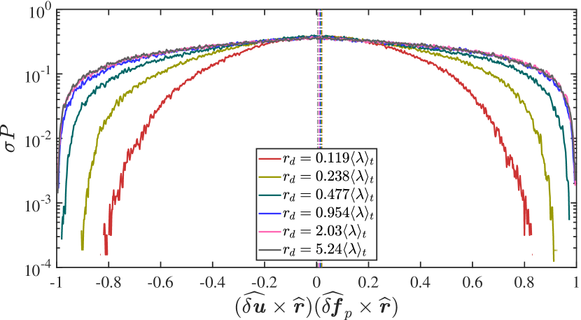
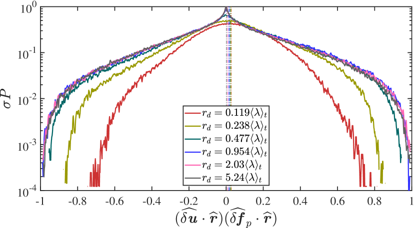
Figure 10: PDFs of (a) (δ𝒖^𝒓^)(δ𝒇p^𝒓^)^𝛿𝒖^𝒓^𝛿subscript𝒇𝑝^𝒓(\widehat{\delta{\bm{u}}}\cdot\hat{\bm{r}})(\widehat{\delta{\bm{f}}_{p}}\cdot\hat{\bm{r}}) and (b) (δ𝒖^×𝒓^)(δ𝒇p^×𝒓^)^𝛿𝒖^𝒓^𝛿subscript𝒇𝑝^𝒓(\widehat{\delta{\bm{u}}}\times\hat{\bm{r}})\cdot(\widehat{\delta{\bm{f}}_{p}}\times\hat{\bm{r}}) obtained from sampling over 𝑿𝑿{\bm{X}}, t𝑡t and 𝒓^^𝒓\hat{\bm{r}} for a given rd=|𝒓|subscript𝑟𝑑𝒓r_{d}=|{\bm{r}}|. The PDFs are normalised by 1/σ1𝜎1/\sigma where σ𝜎\sigma is the standard deviation of the quantity plotted on the abscissa. Different curves correspond to different values of rdsubscript𝑟𝑑r_{d} as shown in the insert. The vertical line indicates the average (a) (δ𝒖^𝒓^)(δ𝒇p^𝒓^)allsubscriptdelimited-⟨⟩^𝛿𝒖^𝒓^𝛿subscript𝒇𝑝^𝒓𝑎𝑙𝑙\langle(\widehat{\delta{\bm{u}}}\cdot\hat{\bm{r}})(\widehat{\delta{\bm{f}}_{p}}\cdot\hat{\bm{r}})\rangle_{all} and (b) (δ𝒖^×𝒓^)(δ𝒇p^×𝒓^)allsubscriptdelimited-⟨⟩^𝛿𝒖^𝒓^𝛿subscript𝒇𝑝^𝒓𝑎𝑙𝑙\langle(\widehat{\delta{\bm{u}}}\times\hat{\bm{r}})\cdot(\widehat{\delta{\bm{f}}_{p}}\times\hat{\bm{r}})\rangle_{all}. Reλt=178subscriptdelimited-⟨⟩𝑅subscript𝑒𝜆𝑡178\langle Re_{\lambda}\rangle_{t}=178 but these plots are very similar for Reλt=80.9subscriptdelimited-⟨⟩𝑅subscript𝑒𝜆𝑡80.9\langle Re_{\lambda}\rangle_{t}=80.9.
Refer to caption
Figure 11: cosϕallsubscriptdelimited-⟨⟩italic-ϕ𝑎𝑙𝑙\langle\cos\phi\rangle_{all}, (δ𝒖^𝒓^)(δ𝒇p^𝒓^)allsubscriptdelimited-⟨⟩^𝛿𝒖^𝒓^𝛿subscript𝒇𝑝^𝒓𝑎𝑙𝑙\langle(\widehat{\delta{\bm{u}}}\cdot\hat{\bm{r}})(\widehat{\delta{\bm{f}}_{p}}\cdot\hat{\bm{r}})\rangle_{all} and (δ𝒖^×𝒓^)(δ𝒇p^×𝒓^)allsubscriptdelimited-⟨⟩^𝛿𝒖^𝒓^𝛿subscript𝒇𝑝^𝒓𝑎𝑙𝑙\langle(\widehat{\delta{\bm{u}}}\times\hat{\bm{r}})\cdot(\widehat{\delta{\bm{f}}_{p}}\times\hat{\bm{r}})\rangle_{all} as functions of rd/λtsubscript𝑟𝑑subscriptdelimited-⟨⟩𝜆𝑡r_{d}/\langle\lambda\rangle_{t}. The three dashed vertical lines indicate the positions on the abscissa of ηtsubscriptdelimited-⟨⟩𝜂𝑡\langle\eta\rangle_{t}, λtsubscriptdelimited-⟨⟩𝜆𝑡\langle\lambda\rangle_{t} and Ltsubscriptdelimited-⟨⟩𝐿𝑡\langle L\rangle_{t}. Reλt=178subscriptdelimited-⟨⟩𝑅subscript𝑒𝜆𝑡178\langle Re_{\lambda}\rangle_{t}=178 but this plot is very similar for Reλt=80.9subscriptdelimited-⟨⟩𝑅subscript𝑒𝜆𝑡80.9\langle Re_{\lambda}\rangle_{t}=80.9.

Some further insight into the interactions between fluctuating pressure gradient and fluctuating interscale energy transfer can be gleaned by using

cosϕ=(δ𝒖^𝒓^)(δ𝒇p^𝒓^)+(δ𝒖^×𝒓^)(δ𝒇p^×𝒓^)italic-ϕ^𝛿𝒖^𝒓^𝛿subscript𝒇𝑝^𝒓^𝛿𝒖^𝒓^𝛿subscript𝒇𝑝^𝒓\displaystyle\cos\phi=(\widehat{\delta{\bm{u}}}\cdot\hat{\bm{r}})(\widehat{\delta{\bm{f}}_{p}}\cdot\hat{\bm{r}})+(\widehat{\delta{\bm{u}}}\times\hat{\bm{r}})\cdot(\widehat{\delta{\bm{f}}_{p}}\times\hat{\bm{r}})\> (9)

where 𝒇ppsubscript𝒇𝑝bold-∇𝑝{\bm{f}}_{p}\equiv-{\bm{\nabla}}p, δ𝒇p^^𝛿subscript𝒇𝑝\widehat{\delta{\bm{f}}_{p}} is the unit vector in the direction of δ𝒇p𝛿subscript𝒇𝑝\delta{\bm{f}}_{p} and δ𝒖^^𝛿𝒖\widehat{\delta{\bm{u}}} is the unit vector in the direction of δ𝒖𝛿𝒖\delta{\bm{u}}. The interest of the decomposition (9) stems from the equality between the volume integral |𝒓|rd4Π(𝑿,𝒓,t)𝑑𝒓subscripttriple-integral𝒓subscript𝑟𝑑4Π𝑿𝒓𝑡differential-d𝒓\iiint\limits_{|\bm{r}|\leq r_{d}}4\Pi(\bm{X},\bm{r},t)d{\bm{r}} and the surface integral |𝒓|=rdδ𝒖𝒓^|δ𝒖|2𝑑𝒓subscripttriple-integral𝒓subscript𝑟𝑑𝛿𝒖^𝒓superscript𝛿𝒖2differential-d𝒓\iiint\limits_{|\bm{r}|=r_{d}}{\delta{\bm{u}}}\cdot\hat{\bm{r}}|{\delta{\bm{u}}}|^{2}d{\bm{r}} which implies that compression events where δ𝒖𝒓^<0𝛿𝒖^𝒓0\delta{\bm{u}}\cdot\hat{\bm{r}}<0 contribute to the forward cascade from large to small scales whereas stretching events where δ𝒖𝒓^>0𝛿𝒖^𝒓0\delta{\bm{u}}\cdot\hat{\bm{r}}>0 contribute to backscatter, i.e. from small to large scales. Hence, the sign of (δ𝒖^𝒓^)(δ𝒇p^𝒓^)^𝛿𝒖^𝒓^𝛿subscript𝒇𝑝^𝒓(\widehat{\delta{\bm{u}}}\cdot\hat{\bm{r}})(\widehat{\delta{\bm{f}}_{p}}\cdot\hat{\bm{r}}) in the decomposition (9) indicates whether the pressure force does or does not act locally in the same way as the local cascade event: (δ𝒖^𝒓^)(δ𝒇p^𝒓^)^𝛿𝒖^𝒓^𝛿subscript𝒇𝑝^𝒓(\widehat{\delta{\bm{u}}}\cdot\hat{\bm{r}})(\widehat{\delta{\bm{f}}_{p}}\cdot\hat{\bm{r}}) is positive when the pressure force and the cascade are both compressing or stretching and is negative when one of the two is compressing and the other stretching.

The other term in the decomposition relates to energy exchanges from one direction to another in 𝒓𝒓{\bm{r}}-space and is therefore not directly related to the cascade. In figure 10 we plot the PDFs of the two terms in the right hand side of (9). The overall shape of the PDF of cosϕitalic-ϕ\cos\phi in figure 8(b) is reflected in the shape of the PDF of (δ𝒖^×𝒓^)(δ𝒇p^×𝒓^)^𝛿𝒖^𝒓^𝛿subscript𝒇𝑝^𝒓(\widehat{\delta{\bm{u}}}\times\hat{\bm{r}})\cdot(\widehat{\delta{\bm{f}}_{p}}\times\hat{\bm{r}}) rather than the PDF of (δ𝒖^𝒓^)(δ𝒇p^𝒓^)^𝛿𝒖^𝒓^𝛿subscript𝒇𝑝^𝒓(\widehat{\delta{\bm{u}}}\cdot\hat{\bm{r}})(\widehat{\delta{\bm{f}}_{p}}\cdot\hat{\bm{r}}). Hence, the wide variability in cosϕitalic-ϕ\cos\phi values and also the gradual reduction of this variability with decreasing length-scales rdsubscript𝑟𝑑r_{d} within the inertial and dissipation ranges seem to mostly reflect directional rather than inter-scale effects in 𝒓𝒓{\bm{r}}-space.

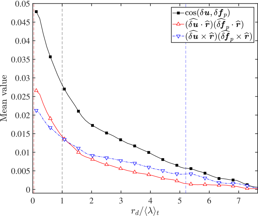
The mean values (δ𝒖^𝒓^)(δ𝒇p^𝒓^)allsubscriptdelimited-⟨⟩^𝛿𝒖^𝒓^𝛿subscript𝒇𝑝^𝒓𝑎𝑙𝑙\langle(\widehat{\delta{\bm{u}}}\cdot\hat{\bm{r}})(\widehat{\delta{\bm{f}}_{p}}\cdot\hat{\bm{r}})\rangle_{all} and (δ𝒖^×𝒓^)(δ𝒇p^×𝒓^)allsubscriptdelimited-⟨⟩^𝛿𝒖^𝒓^𝛿subscript𝒇𝑝^𝒓𝑎𝑙𝑙\langle(\widehat{\delta{\bm{u}}}\times\hat{\bm{r}})\cdot(\widehat{\delta{\bm{f}}_{p}}\times\hat{\bm{r}})\rangle_{all} are both positive at all scales rdsubscript𝑟𝑑r_{d} smaller than Ltsubscriptdelimited-⟨⟩𝐿𝑡\langle L\rangle_{t}, and are in fact increasing with decreasing scale in this range (see figure 11). It is clear that the small positive value of cosϕallsubscriptdelimited-⟨⟩italic-ϕ𝑎𝑙𝑙\langle\cos\phi\rangle_{all} results from small positive values of both (δ𝒖^𝒓^)(δ𝒇p^𝒓^)allsubscriptdelimited-⟨⟩^𝛿𝒖^𝒓^𝛿subscript𝒇𝑝^𝒓𝑎𝑙𝑙\langle(\widehat{\delta{\bm{u}}}\cdot\hat{\bm{r}})(\widehat{\delta{\bm{f}}_{p}}\cdot\hat{\bm{r}})\rangle_{all} and (δ𝒖^×𝒓^)(δ𝒇p^×𝒓^)allsubscriptdelimited-⟨⟩^𝛿𝒖^𝒓^𝛿subscript𝒇𝑝^𝒓𝑎𝑙𝑙\langle(\widehat{\delta{\bm{u}}}\times\hat{\bm{r}})\cdot(\widehat{\delta{\bm{f}}_{p}}\times\hat{\bm{r}})\rangle_{all}, the former being significantly larger than the latter. The fact that (δ𝒖^𝒓^)(δ𝒇p^𝒓^)allsubscriptdelimited-⟨⟩^𝛿𝒖^𝒓^𝛿subscript𝒇𝑝^𝒓𝑎𝑙𝑙\langle(\widehat{\delta{\bm{u}}}\cdot\hat{\bm{r}})(\widehat{\delta{\bm{f}}_{p}}\cdot\hat{\bm{r}})\rangle_{all} is small but positive means that there is a small tendency for the pressure force to act in accordance with the local interscale energy transfer on average, i.e. it has a compressing effect when the interscale transfer is down the scales and a stretching effect when the interscale transfer is up the scales. The opposite happens too, but slightly less often. This small imbalance creates an average picture for the terms in equation (9) which, when combined with the negative average value of ΠΠ\Pi, suggests an average interscale energy transfer from large to small scales that is accompanied by a small compressive effect by the pressure forces.

The fluctuating picture, however, is once again significantly different as can be seen from the positive correlation between the fluctuations of cosϕitalic-ϕ\cos\phi and the fluctuations of ΠΠ\Pi in figure 9. We found similar positive correlations (as functions of rd/λtsubscript𝑟𝑑subscriptdelimited-⟨⟩𝜆𝑡r_{d}/\langle\lambda\rangle_{t}) between (δ𝒖^𝒓^)(δ𝒇p^𝒓^)^𝛿𝒖^𝒓^𝛿subscript𝒇𝑝^𝒓(\widehat{\delta{\bm{u}}}\cdot\hat{\bm{r}})(\widehat{\delta{\bm{f}}_{p}}\cdot\hat{\bm{r}}) and ΠΠ\Pi on the one hand and between (δ𝒖^×𝒓^)(δ𝒇p^×𝒓^)^𝛿𝒖^𝒓^𝛿subscript𝒇𝑝^𝒓(\widehat{\delta{\bm{u}}}\times\hat{\bm{r}})\cdot(\widehat{\delta{\bm{f}}_{p}}\times\hat{\bm{r}}) and ΠΠ\Pi on the other (not plotted here for economy of space). Even though the average of every term in equation (9) is positive (albeit small) and the average of ΠΠ\Pi is negative (albeit also small compared to the fluctuations of ΠΠ\Pi), there is some correlation between negative/positive localised values of ΠΠ\Pi and negative/positive localised values of cosϕitalic-ϕ\cos\phi, (δ𝒖^𝒓^)(δ𝒇p^𝒓^)^𝛿𝒖^𝒓^𝛿subscript𝒇𝑝^𝒓(\widehat{\delta{\bm{u}}}\cdot\hat{\bm{r}})(\widehat{\delta{\bm{f}}_{p}}\cdot\hat{\bm{r}}) and (δ𝒖^×𝒓^)(δ𝒇p^×𝒓^)^𝛿𝒖^𝒓^𝛿subscript𝒇𝑝^𝒓(\widehat{\delta{\bm{u}}}\times\hat{\bm{r}})\cdot(\widehat{\delta{\bm{f}}_{p}}\times\hat{\bm{r}}). The fluctuating picture is therefore, partly, opposite to the average one because it contains instances of events with negative ΠΠ\Pi which correlate with negative values of every term in equation (9), in other words a significant number of cases where the pressure force has a stretching effect even though the interscale transfer is most likely down the scales. This is opposite to the average picture presented at the end of the previous paragraph.

5 Conclusions

The average picture of interscale energy transfers in statistically stationary periodic turbulence is very different from the fluctuating picture which hides behind it. Whereas only the interscale energy transfer rate, the energy input rate, the turbulence dissipation rate and the viscous diffusion in two-point separation space feature in the average picture, the fluctuating picture contains intense and intermittent fluctuations of all the terms in the KHMH equation (1), including the time-derivative, transport and pressure-velocity terms, all of which average out to zero. In fact the most intense fluctuations are those of the time-derivative and the transport term, followed closely by the fluctuations of the interscale energy transfer rate and the pressure-velocity term (figure 5). The fluctuations of each one of these four terms are much more intense than the fluctuations of the turbulence dissipation rate which is known to be highly intermittent since the 1950s (Batchelor & Townsend, 1949; Kolmogorov, 1962; Vincent & Meneguzzi, 1991; Frisch, 1995).

More importantly, perhaps, many of these fluctuations are correlated. These correlations result from the sweeping effect and the link between non-linearity and non-locality. The sweeping effect introduces correlations between the time-derivative term 𝒜tsubscript𝒜𝑡\mathcal{A}_{t} and terms having their origin in the convective non-linearity of the Navier-Stokes equation, namely the transport term 𝒯𝒯\mathcal{T}, the interscale energy transfer rate (with a minus sign for a positive correlation) Πscript-Π-\mathcal{\Pi} and 𝒯Π𝒯script-Π\mathcal{T}-\mathcal{\Pi}. It is important to realise that the interscale energy transfer and related cascade dynamics expressed by ΠΠ\Pi decorrelate from the sweeping effect with decreasing length-scales and increasing Reynolds number. In these limits, the sweeping effect’s partial cancellation is assumed mainly or exclusively by the correlation between 𝒜tsubscript𝒜𝑡\mathcal{A}_{t} and 𝒯𝒯\mathcal{T}.

The link between non-linearity and non-locality which exists in incompressible Navier-Stokes flow is expressed in the significant correlations between the pressure-velocity term 𝒯psubscript𝒯𝑝\mathcal{T}_{p} and each of Πscript-Π\mathcal{\Pi}, 𝒯𝒯\mathcal{T} and Π𝒯script-Π𝒯\mathcal{\Pi}-\mathcal{T}. The sweeping and the non-linear/non-local link effects are separate in that 𝒜tsubscript𝒜𝑡\mathcal{A}_{t} and 𝒯psubscript𝒯𝑝\mathcal{T}_{p} are uncorrelated at all scales. In the limit of small length scales larger than the average Taylor micro-scale (i.e. within what might be termed the inertial range at high enough Reynolds number values) and also as the Reynolds number grows, the correlation with the pressure fluctuations via 𝒯psubscript𝒯𝑝\mathcal{T}_{p} is increasingly with the interscale transfer rate Πscript-Π\mathcal{\Pi} and diminishingly with the transport term 𝒯𝒯\mathcal{T}. The fluctuating pressure has therefore an important role to play in the interscale energy transfer and the energy cascade.

The role of the two-point fluctuating pressure force difference on energy exchanges in 𝒓𝒓{\bm{r}}-space and interscale energy transfers in particular is manifest in the geometrical alignments that it has with the two-point fluctuating velocity difference. These alignments can be decomposed in two parts (see equation 9), one directly concerned with interscale, including cascade, events and the other with reorientation events in 𝒓𝒓{\bm{r}}-space. The fluctuating pressure force is involved in both processes and can have a compressing or a stretching effect on either backscatter or forward cascade events in a way that contributes to correlation statistics and even mean values such as those of figure 11.

It is clear that the average picture of the cascade and interscale exchanges in 𝒓𝒓{\bm{r}}-space does not represent much of the actual physical processes involved even in statistically stationary periodic turbulence. It makes little sense to try to model an unrepresentative average picture rather than attempt to directly model the underlying physics which appear when the clouding effects of averages are lifted. In the case of Large Eddy Simulations, for example, it will be important to supplement existing subgrid modelling approaches, which may have some realism in only part of the flow, with models based on conditional statistics and cross-scale correlations involving various processes, including fluctuating pressure forces. Our results concerning fluctuations, intermittency and the presence of relatively rare but powerful events also suggest the need for further studies of two-point correlations between fluctuating velocity gradients, pressure gradients and fluctuating velocities. Such studies directly impact on correlations between fluctuating velocities and fluctuating pressure forces which need to be modelled in Reynolds-Stress-Transport models.

Acknowledgements

We thank Professor Susumu Goto for letting us use his parallelised pseudo-spectral DNS code for periodic turbulence. We also acknowledge support from ERC Advanced Grant 320560.

References

  • Alves Portela et al. (2017) Alves Portela, F., Papadakis, G. & Vassilicos, J. C. 2017 The turbulence cascade in the near wake of a square prism. J. Fluid Mech. 825, 315–352.
  • Aoyama et al. (2005) Aoyama, T., Ishihara, T., Kaneda, Y., M., Yokokawa., Itakura, K. & Uno, A. 2005 Statistics of energy transfer in high-resolution direct numerical simulation of turbulence in a periodic box. J. Phys. Soc. Jpn. 74 (12), 3202–3212.
  • Batchelor & Townsend (1949) Batchelor, G. K. & Townsend, A. A. 1949 The nature of turbulent motion at large wave-numbers. Proc. Roy. Soc. A 199, 238–255.
  • Cerutti & Meneveau (1998) Cerutti, S. & Meneveau, C. 1998 Intermittency and relative scaling of subgrid-scale energy dissipation in isotropic turbulence. Phys. Fluids 10, 928.
  • Cimarelli et al. (2016) Cimarelli, A., Angelis, E. D., Jiménez, J. & Casciola, C. M. 2016 Cascades and wall-normal fluxes in turbulent channel flows. J. Fluid Mech. 796, 417–436.
  • Danaila et al. (2012) Danaila, L., Krawczynski, J. F., Thiesset, F & Renou, B 2012 Yaglom-like equation in axisymmetric anisotropic turbulence. Physica D 241, 216–223.
  • Domaradzki et al. (1993) Domaradzki, J. A., Liu, W. & Brachet, M. E. 1993 An analysis of subgrid-scale interactions in numerically simulated isotropic turbulence. Phys. Fluids A 5, 1747–1759.
  • Duchon & Robert (2000) Duchon, J. & Robert, R. 2000 Inertial energy dissipation for weak solutions of incompressible Euler and Navier–Stokes equations. Nonlinearity 13, 249–255.
  • Frisch (1995) Frisch, U. 1995 Turbulence: The Legacy of A. N. Kolmogorov. Cambridge Univ. Press.
  • Gomes-Fernandes et al. (2015) Gomes-Fernandes, R., Ganapathisubramani, B. & Vassilicos, J. C. 2015 The energy cascade in near-field non-homogeneous non-isotropic turbulence. J. Fluid Mech. 771, 676–705.
  • Goto (2008) Goto, S. 2008 A physical mechanism of the energy cascade in homogeneous isotropic turbulence. J. Fluid Mech. 605, 355–366.
  • Hill (2002) Hill, R. J. 2002 Exact second-order structure-function relationships. J. Fluid Mech. 468, 317–326.
  • Ishihara et al. (2009) Ishihara, T., Gotoh, T. & Kaneda, Y. 2009 Study of high-Reynolds number isotropic turbulence by direct numerical simulation. Annu. Rev. Fluid Mech. 41, 165–180.
  • Kolmogorov (1962) Kolmogorov, A. N. 1962 A refinement of previous hypotheses concerning the local structure of turbulence in a viscous incompressible fluid at high Reynolds number. J. Fluid Mech. 13, 82–85.
  • Linkmann & Morozov (2015) Linkmann, M. F. & Morozov, A. 2015 Sudden relaminarization and lifetimes in forced isotropic turbulence. Phys. Rev. Lett. 115, 134502.
  • Marati et al. (2004) Marati, N., Casciola, C. M. & Piva, R. 2004 Energy cascade and spatial fluxes in wall turbulence. J. Fluid Mech. 521, 191–215.
  • McComb et al. (2015) McComb, W. D., Linkmann, M. F., Berera, A., Yoffe, S. R. & Jankauskas, B. 2015 Self-organization and transition to turbulence in isotropic fluid motion driven by negative damping at low wavenumbers. J. Phys. A: Math. Theor. 48, 25FT01.
  • Piomelli et al. (1991) Piomelli, U., Cabot, W. H., Moin, P. & Lee, S. 1991 Subgrid-scale backscatter in turbulent and transitional flows. Phys. Fluids A 3, 1766.
  • Togni et al. (2015) Togni, R., Cimarelli, A. & Angelis, E. D. 2015 Physical and scale-by-scale analysis of Rayleigh–Bénard convection. J. Fluid Mech. 782, 380–404.
  • Tsinober (2014) Tsinober, A. 2014 An Informal Introduction to Turbulence. Springer Netherlands.
  • Valente & Vassilicos (2015) Valente, P. C. & Vassilicos, J. C. 2015 The energy cascade in grid-generated non-equilibrium decaying turbulence. Phys. Fluids 27, 045103.
  • Vincent & Meneguzzi (1991) Vincent, A. & Meneguzzi, M. 1991 The spatial structure and statistical properties of homogeneous turbulence. J. Fluid Mech. 225, 1–20.