Modeling shape selection of buckled dielectric elastomers

Abstract

A dielectric elastomer whose edges are held fixed will buckle, given sufficient applied voltage, resulting in a nontrivial out-of-plane deformation. We study this situation numerically using a nonlinear elastic model which decouples two of the principal electrostatic stresses acting on an elastomer: normal pressure due to the mutual attraction of oppositely charged electrodes and tangential shear (“fringing”) due to repulsion of like charges at electrode edges. These enter via physically simplified boundary conditions that are applied in a fixed reference domain using a nondimensional approach. The method is valid for small to moderate strains and is straightforward to implement in a generic nonlinear elasticity code. We validate the model by directly comparing simulated equilibrium shapes with experiment. For circular electrodes which buckle axisymetrically, the shape of the deflection profile is captured. Annular electrodes of different widths produce azimuthal ripples with wavelengths that match our simulations. In this case, it is essential to compute multiple equilibria because the first model solution obtained by the nonlinear solver (Newton’s method) is often not the energetically favored state. We address this using a numerical technique known as “deflation”. Finally, we observe the large number of different solutions that may be obtained for the case of a long rectangular strip.

I Introduction

Dielectric elastomers (DEs) are a class of soft and flexible actuating devices that deform when subjected to electric fields. The significant mechanical strains available in DE systems, compared with competitive technologies, has driven their development in numerous contexts, particularly in engineering.O’Halloran, O’Malley, and McHugh (2008) In a number of applications, including pumps,Pelrine et al. (2001); Tavakol et al. (2014); Tavakol and Holmes (2016) loudspeakers,Heydt et al. (2000, 2006) tactile displaysCarpi, Bauer, and De Rossi (2010); Vishniakou et al. (2013) and others Jung et al. (2007); Son et al. (2012) a key component is a purposefully induced buckling instability.

Typical DE setups involve a thin elastomer membrane coated on opposite faces with areas of conducting material, thereby partitioning the surface into electrically “active” and “inactive” regions. A connecting circuit turns the active regions into oppositely charged electrodes. This creates a flexible capacitor in which the intervening dielectric (the elastomer) is apt to deform under the influence of electrostatic forces. The conducting material is fabricated so that it is free to bend and stretch with the elastomer without constraining its movement.

Figure 1(a) shows an example DE geometry in its zero strain configuration, before any electric field $\bm{E}$ has been applied. The medium is a thin cuboid, on which the top electrode can be seen, shaded in gray. Typical materials used in applications are isotropic and incompressible. They produce significant strains in response to applied voltages on the order of kilovolts. Figure 1(b) demonstrates the effect of an applied electric field, in a simple situation in which the lateral sides of the medium are unconstrained. When the voltage is turned on, attractive forces arising from the charge imbalance on the two electrodes push the top and bottom faces of the elastomer together. This compression is coupled to lateral expansion of the film via incompressibility. If instead, the edges of the elastomer are held fixed in space, the active region and surrounding area will buckle out-of-plane as shown in Fig. 1(c). This is an inevitable consequence of the incompressible material preserving its volume under compression of the electrodes. The equilibrium shape adopted by a deformed elastomer is frequently nontrivial and can contain waves or wrinkles.Pelrine et al. (2000); Plante and Dubowsky (2006); Kollosche et al. (2012); Zhu et al. (2012); Bense et al. (2017)

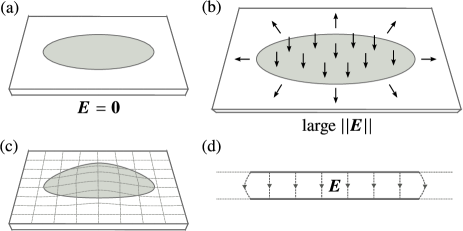
Figure 1: Diagrams of a dielectric elastomer in different situations. In parts (a)–(c) the top electrode (active region) is shaded in gray. (a) DE with no applied electric field ($\bm{E}=\bm{0}$). (b) DE with a strong applied electric field (large $||\bm{E}||$), which causes the elastomer to deform. If the boundaries of the medium are free to move, the material compresses in the thickness direction and extends laterally. (c) If the edges of the medium are instead held fixed, the electrostatic forces between the electrodes force the elastomer to buckle out-of-plane. (d) Two-dimensional cross-section through the middle of the elastomer showing the fringing of the electric field $\bm{E}$. The top and bottom electrodes are represented by thick gray lines. Dashed lines with arrows indicate the direction of the electric field. At the center the field lines are uniformly spaced and normal to the electrodes. At the edges they warp, leaving a small nonzero component of electric field tangent to the medium surface.

Figure 1(d) sketches the electric field lines between the active regions in the ideal undeformed setting. For the most part, the field is constant between the electrodes and electrostatic forces act perpendicular to the top and bottom surfaces of the elastomer. At the conductor edges the field lines become slightly curved because mutual repulsion of like surface charges does not balance, as it does in the center. The result is a fringing field with a small nonzero component tangent to the elastomer surface. This picture also holds approximately for DEs after buckling due to the small interstitial length scale. It should be noted that the electric field schematic is based on an idealized understanding of a classical parallel-plate capacitor and may not always reflect the experimental situation in a DE, where the charge distribution may not be completely uniform. Nevertheless, it suits our purposes here, as will become clear.

The aim of this paper will be to numerically model buckled DE shapes and make direct comparisons with experimental deformation profiles and images. We propose a straightforward approach to DE modeling based on a significant simplification of the underlying physics (including the fringing effect), which is nonetheless able to match nontrivial buckling shapes.

II Experiment

The DEs used in the experiments are made of polyvinyl siloxane (PVS) with a Young’s modulus of $250\pm{}15{}\text{\,}\mathrm{kPa}$, estimated with a standard tensile test on a strip. After mixing equal amounts of base and catalyst, the liquid PVS is spincoated at 500 rpm for 15 seconds and cured, obtaining a solid disc of approximate thickness $150\text{\,}\mathrm{\SIUnitSymbolMicro m}$. The electrodes are made of carbon black powder brushed onto the top and bottom surfaces of the cured polymer using a stencil. They do not change the mechanical properties of the surface. Moreover, the adhesion of the powder is remarkably good and the conductivity of the surface is maintained across the full range of strains that we achieve. The resistivity of the coating is in the order of a few hundred kilohms.

Figure 2 shows the experiment in use.

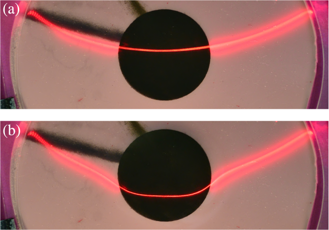
Figure 2: Overhead view of the experiment with circular active region of diameter $30\text{\,}\mathrm{mm}$, before and after actuation. The applied voltages are: (a) $0\text{\,}\mathrm{kV}$ and (b) $4\text{\,}\mathrm{kV}$.

The DE is clamped in a rigid circular polyvinyl chloride (PVC) frame, of diameter $10\text{\,}\mathrm{cm}$ without prestretching the material. In the absence of applied voltage it sags under its own weight. A laser sheet is projected across the diameter of the active region at an oblique incidence angle. Its deflection—monitored using a camera directly above the experiment—is proportional to the deflection of the elastomer surface, allowing us to measure the vertical deformation of the system. At the beginning of the experiment, as the voltage is increased from zero, the membrane sags more and more as the central region grows. However, after a threshold voltage is reached, the system buckles, undergoing an axisymmetric deformation that is strongly localized in the active region. In this paper, we are concerned with capturing deformations after this initial buckling instability, for a variety of active region shapes. For DEs with circular electrodes at still higher voltages, a secondary instability has been observed that causes azimuthal wrinkling at the electrode edges.Bense et al. (2017)

III Model

Anticipating the nontrivial deformations observed in applications, we place our elastomers in a nonlinear elasticity setting. At equilibrium, they obey the elastostatics equation

$$\nabla\cdot\bm{\sigma}(\bm{x})+\bm{b}(\bm{x})=\bm{0},$$ (1)

where $\bm{\sigma}$ is the Cauchy stress tensor, $\bm{b}$ is a body force (density) and the equation is posed over all of the material points $\bm{x}$ that comprise the deformed object. By specifying both an appropriate constitutive law and boundary conditions this equation can be solved for the deformation of the elastic body. In our model, electrostatic forces enter the system via prescribed traction boundary conditions, which we shall detail shortly.

Equation (1) is closed by specifying a particular strain energy density function $W$. We shall use the isotropic Mooney-Rivlin constitutive law, which in its incompressible formulation is

$$W=c_{1}(I_{1}-3)+c_{2}(I_{2}-3),$$ (2)

for phenomenological model parameters $c_{1},c_{2}$, where $I_{1}$ and $I_{2}$ denote the first and second principal invariants of the Cauchy-Green strain tensor. A variety of more sophisticated laws, including the Ogden, Gent, Yeoh and Arruda-Boyce models, have been used in prior DE modeling studies. These capture elastomer strain responses with greater accuracy, especially at large strains.Goulbourne, Mockensturm, and Frecker (2005); Wissler and Mazza (2005, 2007); Xu et al. (2010); Li et al. (2013) However, no prestretch is applied to the elastomers in our experiments and we consider only moderate strains. In this regime we find the Mooney-Rivlin law to be more than adequate for our purposes. Moreover, an advantage to this model is that it only depends on two parameters: $c_{1}$ and $c_{2}$. While elastomers can exhibit viscoelastic properties,Sommer-Larsen and Larsen (2004); Plante and Dubowsky (2007) we shall work in the static setting only and therefore need not consider viscoelasticity here.

We account for the effect of gravity with a constant body force density $\bm{b}$ that acts vertically downwards. It has magnitude $\rho g$, where $\rho$ is the material density (assumed to be constant) and $g$ is gravitational acceleration. This is the only body force that appears in the model.

Finally and most importantly, we model the electrostatic forces present in the system, due to the surface charge distributions on the electrodes. These dictate components of the Cauchy stress across the surfaces of the elastic medium and hence the boundary conditions for Eq. (1). Specifically, if an (area) force density $\bm{\tau}$ impinges on the surface of the deformed body with unit normal $\bm{n}$, then $\bm{\sigma}\bm{n}=\bm{\tau}$. The traction vector $\bm{\tau}$ is determined by modeling considerations.

The principal traction is due to attractive forces between the oppositely charged electrodes. The electrostatic pressure (force density) $p$ between charged surfaces held at a voltage $V$ and at a separation distance $D$ is

$$p=-\frac{1}{2}\epsilon\left(\frac{V}{D}\right)^{\!2}\!\!,$$ (3)

where $\epsilon$ is the permittivity of the region between the charges. This dictates the Cauchy stress acting in the surface normal direction within the active regions.

Towards the edges of the active regions, the electrostatic force on the charge distribution has an additional component that is tangent to the surface of the elastomer film. This arises because the repulsive forces between like charges there are not balanced, as they are in the center. This is indicated in Fig. 1(d), which shows the resultant fringing of the electric field lines at the edges. The tangential forces are small, compared with the normal attraction between the electrodes. Nevertheless, they cause the compliant electrodes to stretch and pull on the material to a certain extent.

In this work, we make the simplifying assumption that the above surface forces can be effectively captured by two regions of constant traction corresponding to the normal pressure and tangential fringing effect. A schematic of our approach is shown in Fig. 3.

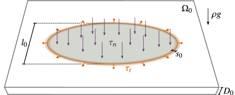
Figure 3: Schematic of the model reference configuration $\Omega_{0}$, showing the application of normal pressure $\tau_{n}$ (purple arrows), tangential traction $\tau_{t}$ (orange arrows), body force density $\rho g$ and the important length scales $D_{0}$, $l_{0}$ and $s_{0}$.

While the electrostatic forces are physically manifest on the surfaces of the deformed body, in practice our numerical simulations use a standard Lagrangian coordinate system corresponding to a fixed, zero-strain reference domain $\Omega_{0}$, as seen in the figure. Hence, Eq. (1) and its boundary conditions must be referred back to this configuration. Specifically, we solve

$$\nabla\cdot\bm{S}(\bm{X})+\bm{b}_{0}(\bm{X})=\bm{0},$$ (4)

where $\bm{S}$ is the (first) Piola-Kirchhoff stress tensor and $\bm{b}_{0}$ is the body force. These quantities are $\bm{\sigma}$ and $\bm{b}$ respectively, written in the Lagrangian frame and are defined over all reference points $\bm{X}\in\Omega_{0}$. Spatial derivatives in Eq. (4) are taken with respect to the reference co-ordinates. The traction boundary condition in this setting is $\bm{S}\bm{N}=\bm{\tau}_{0}$, where $\bm{N}$ is the unit normal vector field on the surface of $\Omega_{0}$. Specification of the reference traction vector $\bm{\tau_{0}}$ is the point at which electrostatic forces enter our model.

The normal electrostatic pressure is set by a constant traction at the top and bottom electrode surfaces of magnitude $\tau_{n}$, directed into the reference material body. The tangential fringing effect is applied in a small annular neighborhood of width $s_{0}$, along the active region perimeter (see Fig. 3). Its magnitude $\tau_{t}$ is constant across this region and its direction is given by the outward normal to the boundary of the annulus. The sum of these two orthogonal vectors at each point comprises the model reference traction $\bm{\tau_{0}}$. It is important to note that in the physical system, the two traction directions lie perpendicular and tangent to the surface of the deformed configuration. By posing them in the Lagrangian frame, we introduce a computationally convenient assumption that is only reasonable when strains are not too large. The values of $\tau_{n}$ and $\tau_{t}$ will be discussed momentarily.

In addition to the width $s_{0}$, there are two important length scales present in the model: the thickness of the unstrained domain $D_{0}$ and the characteristic length of the active region $l_{0}$. The exact definition of $l_{0}$ depends on the shape of the particular active region. In the case of the circle, it refers to the diameter.

For a particular DE configuration, any ratio of electrostatic force components will not change if the potential difference across the plates is altered. This is simply because the electrostatic equations are linear. Therefore, the ratio $\tau_{t}/\tau_{n}$ seems like a natural candidate for a dimensionless parameter that determines the relative strength of the tangential traction applied in the model. However, a better choice is

$$\kappa\coloneqq\frac{s_{0}}{D_{0}}\frac{\tau_{t}}{\tau_{n}},$$ (5)

which takes into account the length scales of the problem. To see why this is necessary, let us consider a potential difference $V$ between the active surfaces in the undeformed geometry of Fig. 3. We know from Eq. (3) that the normal pressure on each surface scales with $(V/D_{0})^{2}$. Likewise, it may be shown (e.g. using the Maxwell stress tensor) that the fringing force at the active region edges scales with $V^{2}/D_{0}$. The corresponding quantity in our model is $s_{0}\tau_{t}$. Therefore, electrostatics implies that $s_{0}\tau_{t}/D_{0}\tau_{n}$ should be constant with respect to changes in $D_{0}$. This scaling might cease to hold in cases where $D_{0}$ becomes comparable to $l_{0}$, but in all cases we consider $D_{0}\ll l_{0}$.

In the system with deformations, the fringing force $f_{t}$ and normal pressure $p$ will be such that $f_{t}/Dp$ is constant, where $D$ the deformed thickness. To keep this constant in our model, it would be strictly necessary to apply a correction, allowing both $\tau_{t}/\tau_{n}$ and the directions of the applied tractions to vary with the deformed geometry. Whilst we have investigated such an approach, it is fundamentally more complicated and does not appear to be any more predictive for the phenomena considered in this study. Hence, we have opted for the simplicity of maintaining constant $\kappa$, as defined in Eq. (5).

Through the dimensionless parameter $\kappa$, we dictate the relative strength of the tangential fringing force applied in the model in a geometry-independent way. Note that $\kappa=0$ means no tangential shear and that larger $\kappa$ corresponds to a larger relative strength of $\tau_{t}$. The value of $\kappa$ is investigated in Sec. V. An implicit, but reasonable assumption in defining $\kappa$ the way we do is that solutions to the model system are not significantly affected by the width $s_{0}$, provided that $s_{0}$ is sufficiently small relative to $D_{0}$ and $l_{0}$. This was verified in detail for the $3\text{\,}\mathrm{kV}$ result presented later in Fig. 5. In practice, we observe that for the thin simulation domains considered herein, setting $s_{0}$ smaller than $l_{0}$ is all that is essential. Indeed, it was necessary for such geometries that $s_{0}$ be comparable to $D_{0}$ in order to ensure that $s_{0}$ covered a sufficient number of points in the spatial discretization of Eq. (4).

The above treatment is a deliberately straightforward and practical attempt to access some of the shapes adopted by buckling DEs. It is worth reiterating here that while it is physically motivated, our model is a simplification of the full physics. The complete picture is very complicated, since it involves a spatially-varying charge distribution whose equilibrium configuration is coupled to the mechanical deformation. Numerous prior studies have therefore opted to solve electrostatic equations and an elasticity model (or viscoelasticity model) in concert.Gao, Tuncer, and Cuitiño (2011); Park et al. (2012); Vertechy et al. (2012); Khan, Wafai, and El Sayed (2013); Klinkel, Zwecker, and Müller (2013); Park et al. (2013); Henann, Chester, and Bertoldi (2013); Vogel et al. (2014); Seifi and Park (2016); Wang et al. (2016) Further detail may be added to the physical picture by accounting for complex interactions arising from polarization of the dielectric and strain-dependent permittivity.Zhao, Hong, and Suo (2007); Zhao and Suo (2008a)

Of particular relevance to our study is the work of Vertechy et al. Vertechy et al. (2012) who considered ‘diaphragm actuators’—buckled circular electrodes within a rigid inactive region. By solving for the electric field both inside the DE and in the surrounding free space, fully coupled with the elastostatic problem, they were able to accurately match experimentally observed displacements. Also notable is the recent observation by Wang et al. Wang et al. (2016) of a (simulated) instability in a diaphragm actuator, similar in character to both the secondary instability of Ref. [Bense et al., 2017] and the wavy patterns that we demonstrate below for annular electrodes.

A simpler modeling approach, derived from the field theory of Suo et al. Suo, Zhao, and Greene (2008) treats the electric field in the Lagrangian frame as constant and perpendicular to the electrodes, its effect on the mechanical stress mediated via a free-energy function defined throughout the material. This level of detail can be sufficient to capture many out-of-plane deformations and instabilities well.Zhou et al. (2008); Zhao and Suo (2008b) Another way to simplify matters (at least computationally speaking) is to reduce the underlying equations to two spatial dimensions. This was used in Ref. [O’Brien et al., 2009] to model DEs attached to frames that bend and curl when activated.

By making the various simplifications detailed above, we sacrifice a certain degree of precision in favor of a more conceptually straightforward model. We argue that there are only two electrostatic effects of principle importance: the normal pressure and the fringing traction. Moreover, we are content to treat these in a fixed reference frame, independent of medium deformation. When applying our model, we use a nondimensional approach, explained in Sec. V. This means that we need not worry about matching the effective pressure with the exact voltage and deformed material thickness. Instead, model parameters are fitted such that the applied tractions scale in a manner consistent with Eq. (3).

IV Methods

We perform nonlinear elasticity simulations using the finite element continuum mechanics solvers from the Chaste software libraries,Mirams et al. (2013) which provide an incompressible nonlinear elasticity implementation that we modified for our own purposes. The nonlinear solver is a damped Newton’s method and the linear solver is GMRES with PETSc’s additive Schwarz preconditioner, using LU factorization blocks.Balay et al. (2017) The deformation map is solved on a zero-strain reference domain $\Omega_{0}$, as depicted in Fig. 3, using tetrahedral quadratic elements. Meshes are constructed using Gmsh,Geuzaine and Remacle (2009) with a minimum of two layers of tetrahedra in the thickness direction. To reduce the number of degrees of freedom these are refined more at the active region and towards the center where most of the strain occurs. Furthermore, we allow elements in the reference domain to be longer in the transverse direction than they are in their thickness. The ratio of these respective dimensions is approximately $1.5:1$ near the active regions and $10:1$ by the outer Dirichlet boundaries where there is very little deformation. In spite of these optimizations, the aspect ratios of the physical system dictate that even the coarsest possible meshes have many elements—typically our simulations use on the order of $10^{5}$ degrees of freedom.

IV.1 Multiple solutions

The elastostatics equation [Eq. (1)] can have multiple solutions. Consequently, there may be many different shapes that an elastomer can adopt in which the material is in equilibrium with the external forces imposed on it. This presents us with a problem when attempting to predict the shape of a DE: the solution that nature selects may not be the one that we happen to find using our nonlinear solver. To address this issue, we implemented an algorithm called “deflation”, whose use in the context of numerical PDE solving is due to Farrell et al.Farrell, Birkisson, and Funke (2015)

The basic idea behind deflation is to factor out solutions from a PDE system that are already known. In our case, we seek the zeros of a nonlinear operator $\mathcal{F}$ defined by $\mathcal{F}(\bm{u})=\nabla\cdot\bm{S}(\bm{u})+\bm{b}_{0}$, subject to the boundary conditions of our model. Suppose that we have found solutions $\bm{u}^{1},\ldots,\bm{u}^{n}$ already. Then we solve the deflated system

$$\mathcal{G}(\bm{u};\bm{u}^{1},\ldots,\bm{u}^{n})\coloneqq\left(\alpha+\sum_{i=1}^{n}\frac{1}{||\bm{u}-\bm{u}^{i}||^{q}}\right)\mathcal{F}(\bm{u})=\bm{0}$$ (6)

for some $\alpha,q>0$. The deflated system has the same solution set as $\mathcal{F}(\bm{u})=\bm{0}$, less the known solutions $\bm{u}^{1},\ldots,\bm{u}^{n}$. Any solution that we find to $\mathcal{G}(\bm{u})=\bm{0}$ is therefore a new equilibrium state for the DE. The inclusion of the parameter $\alpha$ dissuades the numerical method from improperly minimizing the residual of $\mathcal{G}$ below the solver tolerance by pushing intermediate guesses further and further from the known solutions.

The procedure to solve Eq. (6) was implemented using PETSc.Balay et al. (2017) The augmentation of the nonlinear operator results in a rank-one update to the system Jacobian, causing it to lose its sparsity. Consequently, whenever it is needed its application is performed in terms of the Jacobian of the original system via matrix-free methods. Similarly, the preconditioner is implemented matrix-free and is computed via the original preconditioner using the Sherman-Morrison formula as suggested in Ref. [Farrell, Birkisson, and Funke, 2015]. Below, we give some practical details concerning how deflation was used to find multiple DE shapes.

Controlling the order of the singularities in the deflated system with $q$ affects how close any additional candidate solutions can get to $\bm{u}^{1},\ldots,\bm{u}^{n}$, as does varying $\alpha$. Selection of these parameters can greatly alter which solutions can be found by the nonlinear solver. Unfortunately, there is not currently a way to work out a priori what good choices of $\alpha$ and $q$ will be. In the situations where deflation was used we have aimed to maximize the number of solutions obtained by scanning through the $(\alpha,q)$-parameter space. To do this, whenever deflation is used in this work, we fix $q=1.5$ and try many different $\alpha$ values in the range $(0,1]$. (Whilst it would be more comprehensive to scan through a range of exponents as well, this is much more time consuming and was found to be a comparatively less effective way to locate additional solutions.) The exact values of the shifts used are not as important as the need to cover a range encompassing different orders of magnitude. We begin deflation with an initial $\alpha_{0}$, typically in the range $[0.5,1]$ and find successive solutions until the nonlinear solver fails (e.g. due to exceeding the maximum allowed iterations). Each time a new solution is found, it is used as the new initial condition for the solver, after applying a small perturbation to ensure that the deflated operator is finite. After exhausting the solutions that we can find with the initial $\alpha_{0}$, we continue, scanning through a geometric progression of shifts $\alpha_{n}:=\tilde{r}\alpha_{n-1}$, until $\alpha_{n}<\alpha_{\mathrm{min}}$, whereupon deflation is halted. For the systems considered in this paper, $\tilde{r}=2/3$ and $\alpha_{\textrm{min}}=$5\text{\times}{10}^{-3}$$ have been used. At higher values of $\alpha$ the nonlinear solver stays near to the previously deflated solutions since the non-deflated part of the system Jacobian is more significant with respect to the deflated part. As $\alpha$ decreases, more remote solutions become accessible, often at the expense of those with shapes that are structurally close to the deflated ones. For small values of $\alpha$, Newton’s method may take very large steps that decrease the residual of deflation operator, but not the residual of the original system. This can cause numerical instabilities if it produces an intermediate guess which is highly strained. To avoid this, we set an upper limit on the original system residual which, if reached, causes the algorithm to reset the initial condition and move on to the next $\alpha_{n}$. Finally, we note that after a solution has been deflated, this does not prevent Newton’s method from taking steps towards it. In general, the solver is not guaranteed to find a region where it will converge quadratically to a new solution and can spend a long time approaching already-deflated results. It is not uncommon for the method to take more than 100 iterations to converge. To catch most of the solutions, we allow for a maximum of 300 iterations.

In addition to finding solutions with deflation, we were able to find a few additional equilibria using parameter continuation. In this regard, the most useful control parameter is $\kappa$. Starting from an initial solution with $\kappa=\kappa_{0}$, we gradually increment or decrement $\kappa$ until the system adopts a qualitatively different shape. Then continuing $\kappa$ gradually in the reverse direction may produce a distinct solution. The interpretation of this procedure is that the system passed a bifurcation point, uncovering a new solution branch, which we can trace back to $\kappa_{0}$.

Given a set of distinct solutions, it is desirable to determine which will be preferred by the physical system. The potential energy $\Pi$ of the DE is given by integrating the strain energy density over the whole body, minus the work done by the body forces and tractions. This is

$$\Pi(\bm{u})=\int_{\Omega_{0}}W(\bm{u})\,dV-\int_{\Omega_{0}}\bm{b}_{0}\cdot\bm{u}\,dV-\int_{\partial\Omega_{0}}\bm{\tau}_{0}\cdot\bm{u}\,dA,$$ (7)

where $\bm{u}$ is a function that gives the displacement of a material point, relative to its position in the undeformed configuration $\Omega_{0}$, and $\bm{\tau}_{0}$ is the field of tractions on the domain boundary. We perform these integrations numerically over the discretization mesh that we use to solve Eq. (1). This allows us to calculate the minimum energy solution from the shapes found.

V Results

V.1 Circular active region

Before delving into the details of matching simulations with experiment, we present a representative simulation of a buckled DE with applied normal and tangential tractions. Figure 4(a) shows a solution for a circular disc-shaped elastomer with a circular active region at the center.

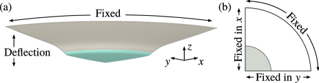
Figure 4: (a) Oblique view of a typical deformed configuration for a thin disc with circular active region, showing the overall deflection and localized buckling in the active region, which is shaded in cyan. The inactive part is shaded in light gray and the fixed outer edge of the domain is indicated. Only a quarter of the geometry is simulated—the rest is accounted for via boundary conditions which enforce reflection symmetry in the planes $x=0$ and $y=0$. The diameter of the full geometry is $666\nicefrac{{2}}{{3}}D_{0}$ and the diameter of the full active region is $l_{0}=266\nicefrac{{2}}{{3}}D_{0}$. Other parameters are: $\kappa=0.6$, $\tau_{n}=0.5$, $\tau_{t}=$0.0225$$ and $\rho g=0$. (b) Schematic showing the boundary conditions for the circular disc.

The plot is an oblique view of the deformed configuration, with the active region indicated. To save computational effort, we solve the elastostatics equation for only a quarter of the axisymmetric geometry. Consequently, we see a cross-section of the elastomer in the figure and may easily inspect the solution’s out-of-plane deflection. Starting from the outer edge, the profile slopes gently downwards, before an abrupt transition at the edge of the active region where the gradient becomes much steeper. In the bulk of the active region however, the profile levels out and is close to flat. Figure 4(b) indicates the boundary conditions used. The outer arc of the disc is fixed in place with a Dirichlet condition. The other two edges are free to move both in the radial direction and out-of-plane ($z$-direction), while their remaining degree of freedom is fixed. Solutions for these boundary conditions correspond to solutions to the full problem with at least reflection symmetry in the $x$ and $y$ directions. (In practice our circular-electrode solutions possess continuous rotational symmetry in the $xy$-plane.)

In each of the following cases the geometry of the simulation is set such that the dimensions of the finite element mesh equal those of the experiment. We set our model parameters using a nondimensional approach, taking the undeformed material thickness $D_{0}$ to be the natural length unit for the system. We choose $s_{0}$ such that the tangent force is applied over a width of at least two (quadratic) finite elements. In all results, $10\leq s_{0}/D_{0}\leq 20$. After fixing the geometry, there are five free parameters in the model: the Mooney-Rivlin constants $c_{1}$ and $c_{2}$, the density $\rho$ and the tractions $\tau_{n}$ and $\tau_{t}$. We are free to choose $c_{1}=1$, since it may be easily verified that any solution to the governing equations satisfies those same equations after rescaling each model parameter $k$ by $k\mapsto\mu k$ for any nonzero constant $\mu$. Moreover, we found that varying the ratio $c_{1}/c_{2}$ had no noticeable effect on the shape of our solutions in any of the contexts studied herein. Hence, we set $c_{1}=c_{2}=1$ throughout. The redundancy of the $c_{2}$ parameter suggests that, at least for the range and type of strains that we consider, a Neo-Hookean constitutive law ($c_{2}=0$) may be sufficient to model the elastomer well.

Figure 5 shows comparison between simulation and experiment for six different applied voltages.

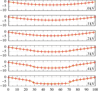
Figure 5: Comparison of experimentally measured deflections with simulation profiles for a succession of increasing voltages: $0\text{\,}\mathrm{kV}1\text{\,}\mathrm{kV}2\text{\,}\mathrm{kV}3\text{\,}\mathrm{kV}4\text{\,}\mathrm{kV}5\text{\,}\mathrm{kV}$. The aspect ratio is $1:1$. Red crosses indicate experimental data points. The experimental geometry used was a thin disc, diameter $100\text{\,}\mathrm{mm}$, thickness $D_{0}=$0.15\text{\,}\mathrm{mm}$$, with centered circular electrodes, $l_{0}=$40\text{\,}\mathrm{mm}$$. Yellow lines are midlines through a model simulation with corresponding geometric parameters and $\kappa=0.6$ in each case. The gravitational body force is $\rho g=$3.6\text{\times}{10}^{-4}$$ throughout. Applied tractions across the different voltages are (to 4 significant figures): $\tau_{n}=\tau_{t}=0$ for $0\text{\,}\mathrm{kV}$; $\tau_{n}=$0.018\,57$$, $\tau_{t}=$8.538\text{\times}{10}^{-4}$$ for $1\text{\,}\mathrm{kV}$; $\tau_{n}=$0.076\,33$$, $\tau_{t}=$3.435\text{\times}{10}^{-3}$$ for $2\text{\,}\mathrm{kV}$; $\tau_{n}=$0.18$$, $\tau_{t}=$8.1\text{\times}{10}^{-3}$$ for $3\text{\,}\mathrm{kV}$; $\tau_{n}=$0.347$$, $\tau_{t}=$0.015\,61$$ for $4\text{\,}\mathrm{kV}$; $\tau_{n}=$0.6176$$, $\tau_{t}=$0.027\,79$$ for $5\text{\,}\mathrm{kV}$.

Each plot shows the midline of a numerical solution restricted to the $y=0$ plane, together with points of experimentally measured deflection. The experimental data covers the full diameter of the elastomer. Therefore, the simulation midline in this case is mirrored across the axis of symmetry in the plots. When taking measurements in the experiment, the deflection of the surface means that the laser does not travel exactly through the elastomer diameter. Consequently, the experimental data does not extend fully to the edges of the simulation domain. In order for the experiment and model geometries to match (in particular the electrode radii), it is necessary to apply a correction. Therefore, we adjust the horizontal scale of the experimental points by a small amount (4.2%), chosen such that the edges of the laser trajectory match those of the simulation domain.

The procedure for fitting the model parameters is as follows. First, the profile of the elastomer with no applied voltage is measured. In this case, there is only one free model parameter—the material density—which is adjusted in the simulations until the amplitude at the center matches the experiment. Next, voltage is applied in the experiment to produce significant additional strain in the elastomer and the profile is measured again, in this case at $3\text{\,}\mathrm{kV}$. The nontrivial shape adopted by the data points allows us to fit both $\tau_{n}$ and $\tau_{t}$ concurrently and thereby determine $\kappa$ [Eq. (5)]. This is because the amplitude of the active region deflection and the overall shape at the electrode boundary are effectively independent of one another in the model. The amplitude of deflection corresponds roughly to the total applied traction and while the shape at the electrode boundary is determined by the ratio $\tau_{t}/\tau_{n}$. We will return to this point shortly. After making an initial guess of their approximate magnitudes and ratio, $\tau_{n}$ and $\tau_{t}$ are incrementally increased or decreased (in concert) until the solution amplitude matches the experiment. Next, to match the profile shape, $\tau_{t}$ is incremented or decremented. Small discretionary adjustments to the tractions are then made to improve agreement further. From this point on, both $\rho$ and $\tau_{t}/\tau_{n}$ are considered to be fixed.

We know from Eq. (3) that the normal pressure $p$ is proportional to $(V/D)^{2}$. The two fitted results at $0\text{\,}\mathrm{kV}3\text{\,}\mathrm{kV}$ uniquely determine the coefficient of proportionality. However, since $p$ depends on the deformed thickness $D$, the amount of normal pressure for a given voltage is coupled to the solution. Furthermore, we model $p$ with the applied traction $\tau_{n}$ in the Lagrangian frame and the pressure that a given $\tau_{n}$ corresponds to in the deformed body also depends on $D$. Specifically, one can show that $\tau_{n}\propto p/D\propto V^{2}/D^{3}$. Therefore, for the remaining voltages in Fig. 5, we determine $\tau_{n}$ using an iterative procedure. Each step enforces the proportionality condition using the deformed thickness (taken at the center point) of the previous iteration. A similar approach was used in Ref. [Wissler and Mazza, 2007]. Successive iterations converge rapidly to a normal pressure that scales correctly with the electric field in the experiment. The applied tractions used in Fig. 5 all obey the correct scaling relation dictated by Eq. (3) to within $1\%$ relative error. Throughout this procedure, $\tau_{t}$ is selected such that $\tau_{t}/\tau_{n}$ (and thus $\kappa$) stays the same.

The profile shapes obtained this way agree extremely well across all the plots, even though the parameters were only fitted using the $0\text{\,}\mathrm{kV}$ and $3\text{\,}\mathrm{kV}$ cases. For voltages greater than or equal to $4\text{\,}\mathrm{kV}$ there are very small discrepancies which may, for instance, be due to the constitutive law used, or the simplified treatment of the forces acting on the elastomer in our model. Nevertheless, even at these higher strains agreement between the model and experiment is good.

For the tractions used in this particular case with a circular active region centered inside a disc, $\tau_{t}/\tau_{n}=0.045$. Taking into account the geometric parameters, this corresponds to $\kappa=0.6$. Since $\tau_{t}$ is so small compared with $\tau_{n}$, one may wonder whether the tangential forces in the model may be neglected altogether. However, despite its magnitude, slight changes in $\tau_{t}$ can have a marked effect on solutions. Indeed, we find that $\kappa=0.6$ fits the experimental data better than either $\kappa=0.58$ or $\kappa=0.62$, though the differences between model profiles are subtle at this level. Figure 6 demonstrates the much more significant effect of changing $\kappa$ by $\pm 0.2$.

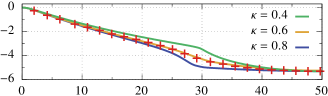
Figure 6: Effect of tangential shear on the shape of model profiles. The vertical axis has been scaled by a factor of 2 to show the variation between the profiles more clearly. Red crosses are data points from the $3\text{\,}\mathrm{kV}$ experiment in Fig. 5. Green, yellow and blue lines are model results with $\kappa=0.4$, $0.6$ and $0.8$ respectively. In each case, the total traction was chosen so that the model profile matched the experimental deflection in the center, at $x=50$. The tractions were as follows: $\kappa=0.4$ used $\tau_{n}=$0.156$$, $\tau_{t}=$4.68\text{\times}{10}^{-3}$$, $\kappa=0.6$ used $\tau_{n}=0.18$, $\tau_{t}=$8.1\text{\times}{10}^{-3}$$ and $\kappa=0.8$ used $\tau_{n}=0.22$, $\tau_{t}=$0.0132$$. All other model parameters match those from Fig. 5.

Here, the $3\text{\,}\mathrm{kV}$ experimental data from Fig. 5 are replotted alongside three model profiles with $\kappa=0.4$, $0.6$ and $0.8$. As $\kappa$ increases, the proportion of tangential force increases. This has two main effects. Increased tension at the edges causes the active region to flatten out and stretch. This in turn modifies the shape at the electrode boundary. Both the $\kappa=0.4$ and $\kappa=0.8$ profiles feature an abrupt change of gradient near the active region edge. Only $\kappa=0.6$ features the smooth transition from inactive to active region that matches the experiment. Thus, for all further results, we use $\kappa=0.6$ unless otherwise stated.

V.2 Annular active region

Another system of experimental interest is shown in Fig. 7.

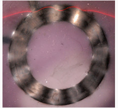
Figure 7: Overhead view of an elastomer experiment with an annular active region, whose geometry corresponds to the simulation in Figs. 8(b) and (c). The inner radius of the annulus is $r_{0}=$17\text{\,}\mathrm{mm}$$, the outer radius is $R_{0}=$25\text{\,}\mathrm{mm}$$ and $D_{0}=$0.15\text{\,}\mathrm{mm}$$. The applied voltage is $3\text{\,}\mathrm{kV}$. Azimuthal ripples are visible on the electrode; their undulation is highlighted by directing a laser across the surface.

In this case, the active region is annular. For sufficiently high applied voltage, this DE readily buckles to produce azimuthal ripples in the active region. Wavelengths measured from the experiment are robust over a range of voltage ($35\text{\,}\mathrm{kV}$) and depend principally on the width of the annulus. In particular, increasing the applied voltage from the onset of this instability only acts to increase the overall deflection of the DE and amplitude of its ripples. These ripples in the active region are distinct from the much smaller wavelength wrinkles that result from a pull-in instability.Plante and Dubowsky (2006)

In the annular case, the active region has two edges. Consequently, there is an additional tangential fringing effect pointing radially inward. A diagram of the simulation domain and imposed tractions is shown in Fig. 8(a).

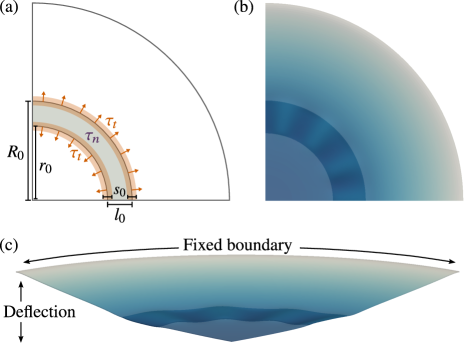
Figure 8: (a) Diagram showing the top/bottom surface of the model setup for a circular disc with annular active region. Compressive normal pressure $\tau_{n}$ is applied into the page across the shaded gray area. Tangential surface tractions $\tau_{t}$ are applied at both boundaries of the active region in the two orange areas shown. Important length scales are labeled: the inner radius $r_{0}$ and outer radius $R_{0}$ of the active region annulus, its width $l_{0}$ and the width $s_{0}$ over which the tangential traction is applied. (b) Example result from the setup depicted in part (a). The blue coloration indicates deformation in the negative $z$-direction. Deeper blue means that a point is displaced further below its original position in the flat reference configuration. The active region is indicated as an area of comparatively darker shading. The geometry is set to match an experiment with $r_{0}=$17\text{\,}\mathrm{mm}$$, $R_{0}=$25\text{\,}\mathrm{mm}$$, $D_{0}=$0.15\text{\,}\mathrm{mm}$$ and diameter $100\text{\,}\mathrm{mm}$. Other model parameters are: $\kappa=0.6$ and $\rho g=$3.6\text{\times}{10}^{-4}$$. (c) Oblique view of the result in part (b) showing the overall deflection of the DE and the azimuthal ripples in the active region.

The two fringing regions are both modeled with width $s_{0}$ centered at the inner and outer radii of the electrode annulus, labeled $r_{0}$ and $R_{0}$ respectively. The characteristic length scale of the active region $l_{0}$ in this case refers to the width of the annulus.

We use the same boundary conditions as for the circular disc [see Fig. 4(b)], simulating only a quarter segment of the whole system in order to save computational cost. However, in this case, our buckled DEs do not possess continuous rotational symmetry. Therefore, it is important to note that these conditions place constraints on the range of admissible wavelengths. In cases where the wavelengths are particularly large, we increase our domain size to half a disc, ensuring that the simulation can always fit many ripples within the given domain.

Figures 8(b) and (c) show overhead and oblique views of a simulated result for an annulus of width $53\nicefrac{{1}}{{3}}D_{0}$. The dimensions of this simulation correspond to the experiment photograph in Fig. 7. From visual inspection one sees a qualitative agreement between the experiment and simulation, both in the overall deformation profile and the character of the ripples.

As mentioned above, there may be many distinct solutions to the elastostatics equation [Eq. (1)] that are not related by symmetry. Indeed, for this system it is possible to find solutions with different azimuthal wavelengths. The wavelength selected by the physical system would typically be the one which minimizes the energy, given in Eq. (7). This is not generally the solution first discovered by our nonlinear solver. To overcome this problem, we use the deflation method, described in Sec. IV.1, to find as many different solutions as we can. The result pictured in Figs. 8(b) and (c) is the minimum energy solution of four different equilibrium configurations computed by this technique. Likewise, the annular active region results below are all energy minima from sets of deflated solutions. However, deflation does not guarantee that every solution will be found. To increase our confidence that these results are close the global minima, we can compare their azimuthal wavelengths with measurements from the experiment.

Figure 9 shows simulations with various annular active region widths.

Figure 9: Deformed configurations for a circular disc with annular active regions of different widths $l_{0}$. Each is the solution found with the lowest energy after deflation. As $l_{0}$ increases, so does the wavelength of ripples in the active region. The extent of the active region in each case is indicated with darker shading. Model parameters are the same as in Fig. 8, save $r_{0}$ which was adjusted for each $l_{0}$ as indicated.

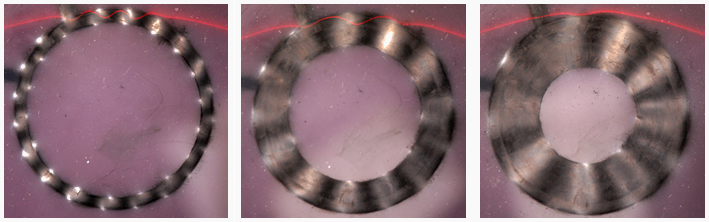
Figure 10: A selection of annular experiments with $R_{0}=$25\text{\,}\mathrm{mm}$$ and different $l_{0}$. The applied voltage is $3\text{\,}\mathrm{kV}$. From left to right: $l_{0}=3,8$ and $12\text{\,}\mathrm{mm}$. The geometries correspond to the first, third and fifth simulations in Fig. 9 respectively.

One sees that as $l_{0}$ increases, the wavenumber observed across the quarter segment decreases. This is observed in experiment: in Fig. 10 we show overhead pictures of the experiment with different annular widths. These correspond to the simulated geometries with $l_{0}=20D_{0}$, $53\nicefrac{{1}}{{3}}D_{0}$ and $80D_{0}$ and may be compared directly with the pictures in Fig. 9. Qualitatively there is good agreement between the two sets of images.

In Fig. 11 we plot both experimental and simulated ripple wavelengths against $l_{0}$ and see more clearly the quantitative agreement between the two.

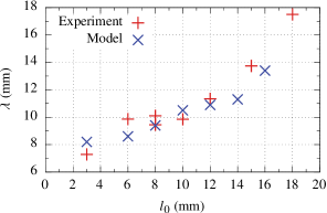
Figure 11: Width $l_{0}$ of annular active region versus observed ripple wavelength $\lambda$ for the experiment and model simulations. The experiment parameters were $D_{0}=$0.15\text{\,}\mathrm{mm}$$ with $R_{0}$ fixed at $25\text{\,}\mathrm{mm}$ and various $r_{0}$ between $7$ and $22\text{\,}\mathrm{mm}$. The applied voltage was $3\text{\,}\mathrm{kV}$.

Wavelengths are calculated in both cases by dividing the circumference of the circle of radius $r_{0}+\tfrac{1}{2}l_{0}$ by the observed wavenumber. The results with $l_{0}=12$, $14$ and $16$ were obtained with a half-disc simulation domain. There is a degree of uncertainty associated with measuring these data points experimentally. Nevertheless, the model does a good job of matching the smaller reported wavelengths in the physical system.

Finally, we verify that $0.6$ is indeed a good choice for $\kappa$, as it was in the case of circular electrodes. Figure 12 plots simulations of the $l_{0}=40D_{0}$ case for $\kappa=0.4,0.6$ and $0.8$.

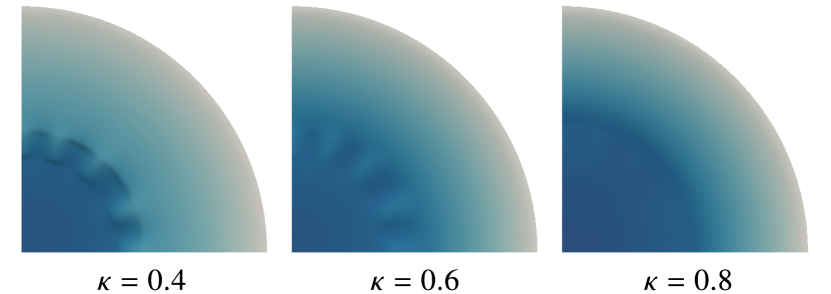
Figure 12: Effect of tangential shear on annular active region simulations. All model parameters match those in Fig. 8, aside from $r_{0}$ which was set to give $l_{0}=40D_{0}$ and $\tau_{t}$ which was varied for different $\kappa$ as labeled.

To produce these solutions, we fix $\tau_{n}=0.32$ and vary $\tau_{t}$ to achieve the desired $\kappa$. Decreasing the amount of tangential shear to $\kappa=0.4$ causes the edges of the active region to crease slightly and the spacing between ripples becomes uneven. Increasing to $\kappa=0.8$ flattens the active region and the ripples disappear. In both cases, the effect on the radial deflection profile is similar to Fig. 6.

V.3 Rectangular active region

A third simple, but important configuration is a long rectangular elastomer with a rectangular active region, as illustrated in Fig. 13(a). Provided that the length of the rectangle is sufficiently greater than its width, this system also readily buckles to produce ripples along its length. This was previously noted by Pelrine et al.Pelrine et al. (2000) Similar ripples in a prestretched DE were also observed by Díaz-Calleja et al.Díaz-Calleja et al. (2013) Our own experimental investigations, while not extensive, indicate that the ripple wavelengths are approximately equal to those observed in an annular active region of the same width.

A schematic of our model setup is shown in Fig. 13(b), alongside a representative result in Fig. 13(c).

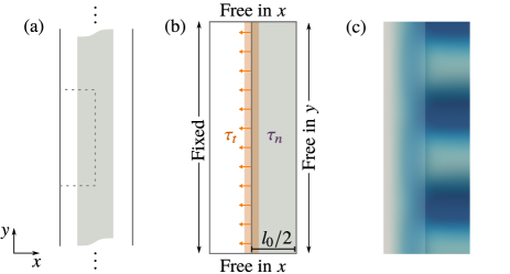
Figure 13: (a) Top-down picture of a rectangular strip DE, with active region shaded in gray. Dots indicate that the elastomer extends far in its lengthwise extent. The dashed gray rectangle shows the region simulated in our computations, which take advantage of symmetries described below. (b) Diagram of the boundary conditions for simulation. Periodic symmetry is enforced at the top and bottom edges. The other two edges implement reflective symmetry in the axis along the right-hand side. See the text for details. Surface tractions $\tau_{n}$ and $\tau_{t}$ are applied in the gray and orange regions respectively, as indicated. The definition of the characteristic width $l_{0}$ for this active region is as labeled. It covers half the simulated domain. (c) An example deformed configuration. The active region is indicated with an area of darker shading. As in the annular case, ripples are present. These follow the direction of the strip’s longer dimension. The model parameters are: $\kappa=0.6$, $\tau_{n}=0.37$, $\tau_{t}=$0.0222$$, $\rho g=0$ and the dimensions are height $H_{0}=250D_{0}$ and width $L_{0}/2=92\nicefrac{{1}}{{2}}D_{0}$.

We consider a rectangular geometry with its width aligned with the $x$-axis and its length aligned with $y$. We assume that deformations are symmetric about the midline in $x$ and so only simulate half the full width. Furthermore we, set the active region to the full length of the domain. This effectively mimics a portion of longer elastomer far from any physical boundaries in $y$. All together this means that the active region extends to the edges of the computational domain on three sides.

The boundary conditions are as follows. The two short edges of the domain are free to move in the $x$ and $z$ directions only. Fixing them in $y$ enforces periodic symmetry. No tangential force is applied in this direction. One of the two long edges is held fixed, corresponding a frame holding the elastomer. The other long edge is free to move in the $y$ and $z$-directions, corresponding to the reflection symmetry about the midline. The dimensions of the simulation domain are height $H_{0}=250D_{0}$ and width $L_{0}/2=92\nicefrac{{1}}{{2}}D_{0}$. The width $l_{0}/2$ of the simulated active region covers half the domain.

Similar to the case of an annular active region, the finite extent of the domain means that some long wavelengths are inaccessible. Guided by the results in the annular case and intuition from experiments with rectangular electrodes, we believe that the domain dimensions chosen are sufficient to capture any important solutions.

We were able to obtain many solutions via deflation for this geometry. These are shown in Fig. 14, with their corresponding energies printed underneath.

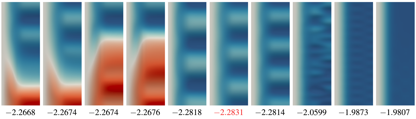
Figure 14: Deflated solutions for a long rectangular strip. $\kappa=0.6$. The blue and red coloration indicate deformation in the $z$-plane. Darker red (blue) means that a point is displaced further above (below) its original position in the flat reference state. Beneath each solution the energy computed using Eq. (7) is printed. Solutions that are equivalent under symmetry to the ones shown have been omitted.

In this case, a variety of interesting solutions can be found. To this end, we omitted the gravitational body force from the model. This encourages the DE to buckle up, as well as down and enables us to find more solutions. In the center of the figure are solutions with regular ripples, analogous to those seen in the annular active region. To the left, there are four solutions composed of a large wavelength mode and smaller ripples. To the right are solutions with higher frequency ripples: one with regular ripples, another with irregular ripples and one with a smooth, mostly flat active region. For each shape shown, reflections in the planes $y=H_{0}/2$ and $z=D_{0}/2$ give solutions that are equivalent under the symmetries of the problem. These have been omitted from Fig. 14. The final two solutions to the right were found using the parameter continuation technique described in Sec. IV.1. The highlighted entry is the minimum energy solution. It is important to note that this was not the first solution to be found by the nonlinear solver. In fact, prior to using deflation, the only configuration accessible was the leftmost solution in Fig. 14, which does not even agree qualitatively with the minimum. Therefore, in this case it was essential to use deflation (or some alternative method) to find multiple solutions and thereby identify the correct equilibrium DE shape. We note that finding a higher-energy solution at lower wavenumber gives us reason to believe that increasing the domain length will not produce a lower energy minimum. Finally, preliminary experimental investigations indicate that the minimum energy numerical solution captures both the wavelength and amplitude of rippling for a rectangular strip.

VI Discussion

We have presented a simplified numerical model for capturing the shape of buckled DE. The electrostatic forces acting on the dielectric are input as boundary conditions to the nonlinear elastostatics equation. We have proposed that the aggregate effect of the applied electric field on the elastomer can be modeled as a normal pressure, due to the attraction between the electrodes, plus a small tangential traction meant to capture the effect of the fringing field at edges of the active regions. The resulting boundary conditions are easily implemented and while they represent a simplification of the underlying physics, they are nonetheless able to produce close fits to experimental data.

The magnitude of the fringing force, relative to the effective pressure is captured by our model in a dimensionless constant $\kappa$. By tuning $\kappa$ to produce solutions best matching experimental deformation profiles, we have found that $\kappa=0.6$. This value proved robust across different applied voltages and different shapes of active regions. The impact that the tangential traction has on solutions is significant, despite its small magnitude. If the effect is left out of the model ($\kappa=0$), we are unable to obtain deformation profiles that are even qualitatively correct.

We have computed deformed solutions for a variety of active regions—circular, annular and rectangular. For the circular and annular cases we have quantitatively compared numerical solutions with experimental observations. In the case of an annular active region, we observe that the elastomer buckles to produce azimuthal ripples, which are localized in the vicinity of the electrodes. Their wavelength increases in proportion with the width of the annulus. This trend is captured well by our model which produces solutions in qualitative agreement with the experiment.

Our approach is quite generic and could be used for a variety of elastomer geometries. Furthermore, the model is, in principle, amenable to arbitrary active region shapes, though some care would need to be taken at any nonsmooth features such as corners. Prestretch may be applied by adjusting the dimensions of the unstrained reference configuration $\Omega_{0}$, relative to the imposed Dirichlet (fixed-displacement) boundary conditions at the domain edges. While we would not necessarily expect our model to be predictive in high-strain regimes, it may be useful in some circumstances. For instance, one effect of prestretch is to nonlinearly increase the buckling threshold.Bense et al. (2017) Although the basic mechanism is clear, the nonlinear dependence of the threshold is not currently understood. Since this phenomenon occurs at low prestretch, a careful application of our model might capture it.

Finally, a key aspect of our study is the computation of multiple solutions. We demonstrate that non-uniqueness of equilibria must be considered whenever model configurations are generated—a fact that has implications for any study of patterns in nonlinear elasticity. In computing a single solution to the elastostatics equation [Eq. (1) or Eq. (4)], one cannot guarantee that it corresponds to the equilibrium shape with the lowest possible potential energy. Indeed, we observe that for a given set of model parameters, the first solution located by our nonlinear solver (damped Newton’s method) is typically not energetically favorable. Consequently, it is desirable to find many different solutions and work out which is favored by the system, either by computing their potential energies via Eq. (7), comparing with experimental data, or using some other physical argument. Deflation is one such technique that can be used to find multiple solutions.Farrell, Birkisson, and Funke (2015) For the annular active region, this was used to find the lowest energy azimuthal wavelength, which was subsequently compared with experimental observations in Fig. 11. Almost all of the model wavelengths reported in our paper come from solutions that were only found after applying the deflation method. In the analogous case of a long rectangular strip, the first solution that we computed does not even qualitatively resemble the minimum. By computing multiple rectangular solutions, we identified many interesting deformation patterns including ripples with different wavelengths, wrinkles and creases.