Exposing and exploiting structure: optimal code generation for high-order finite element methods

Abstract.

Code generation based software platforms, such as Firedrake, have become popular tools for developing complicated finite element discretisations of partial differential equations. We extended the code generation infrastructure in Firedrake with optimisations that can exploit the structure inherent to some finite elements. This includes sum factorisation on cuboid cells for continuous, discontinuous, $H(\mathrm{div})$ and $H(\mathrm{curl})$ conforming elements. Our experiments confirm optimal algorithmic complexity for high-order finite element assembly. This is achieved through several novel contributions: the introduction of a more powerful interface between the form compiler and the library providing the finite elements; a more abstract, smarter library of finite elements called FInAT that explicitly communicates the structure of elements; and form compiler algorithms to automatically exploit this exposed structure.

1. Introduction

Code generation based software tools have become an increasingly popular mechanism for the implementation of complicated numerical solvers for partial differential equations using the finite element method. Examples of such software platforms include FreeFem++ (Hecht, 2012), FEniCS (Logg et al., 2012; Alnæs et al., 2015), and Firedrake (Rathgeber et al., 2016). These software packages enable high-productivity development of reasonably efficient numerical codes. They are most commonly used for low-order finite element discretisations of complicated PDEs, while code for the assembly of high-order finite element discretisations has been predominantly by manually written.

High-order finite element methods, such as the spectral element method (Patera, 1984), combine the convergence properties of spectral methods with the geometric flexibility of traditional linear FEM. Because they provide a larger amount of work per degree-of-freedom, they are also better suited to make use of modern hardware architectures, which exhibit a growing gap between processor and memory speeds. These techniques have been successfully employed in a number of research packages: NEK5000 (Fischer et al., 2008), Nektar++ (Cantwell et al., 2015) and PyFR (Witherden et al., 2014) for computational fluid dynamics, HERMES (Vejchodský et al., 2007) for Maxwell’s equations, EXA-DUNE (Bastian et al., 2014) for porous media flows, pTatin3D (May et al., 2014) for lithospheric dynamics. Hientzsch (2001) implemented an efficient discretisation of Maxwell’s equations using $H(\mathrm{curl})$ conforming spectral elements. However, according to Cantwell et al. (2015), the implementational complexity of these techniques has limited their uptake in many application domains, especially outside academia.

FEniCS and Firedrake depend on the FInite element Automatic Tabulator (FIAT) (Kirby, 2004), a library of finite elements. Since FIAT generally supports finite elements with arbitrary order, FEniCS and Firedrake do in principle support high-order finite element discretisations. However, their implementations have hitherto lacked the optimisations that are crucial at high order, resulting in much slower performance than hand-written spectral element codes. The reason that this deficiency has not been corrected in any of the previous work on improved code generation in FEniCS and Firedrake (Kirby and Logg, 2007; Ølgaard and Wells, 2010; Luporini et al., 2015; Luporini et al., 2017; Homolya et al., 2017) is that the interface which FIAT presents to form compilers prevents the exploitation of the required optimisations.

To implement the necessary optimising transformations, one needs to rearrange finite element assembly loops in ways that take into account the structure inherent to some finite elements. FIAT, however, does not and cannot express such structure, because its interface provides no way to do so. We therefore hereby present FInAT, a smarter library of finite elements that can express structure within elements by introducing a novel interface between the form compiler and the finite element library.

The rest of this paper is arranged as follows. In the remainder of this section we review the relevant steps of finite element assembly, describe the limitations of FIAT in more details, and finally list the novel ideas incorporated in this work. Section 2 introduces FInAT and its structure-preserving element implementations. Section 3 describes the form compiler algorithms implemented in the Two-Stage Form Compiler (TSFC) (Homolya et al., 2017) that exploit the structure of elements to optimise finite element kernels. We verify the results through experimental evaluation in section 4, and section 5 concludes the paper.

1.1. Background

We start with a brief recap of finite element assembly to show how code generation based solutions (e.g., FEniCS and Firedrake) make use of a finite element library such as FIAT. Consider the stationary heat equation $-\nabla\cdot(\kappa\nabla u)=f$ with $\kappa$ thermal conductivity and $f$ heat source on a domain $\Omega$ with $u=0$ on the boundary. Its standard weak form with left-hand side $a(u,v)$ and right-hand side $L(v)$ is given by

(1.1) $$a(u,v) =\int_{\Omega}\kappa\nabla u\cdot\nabla v\,\mathrm{d}x\quad\text{and}$$

(1.2) $$L(v) =\int_{\Omega}fv\,\mathrm{d}x.$$

Such weak forms are defined in code using the Unified Form Language (UFL) (Alnæs et al., 2014). The prescribed spatial functions are often represented as functions from finite element function spaces. In UFL terminology, $v$ and $u$ are called arguments, and $\kappa$, and $f$ are called coefficients of the multilinear forms $a$ and $L$.

For a simpler discussion, we take $\kappa\equiv 1$, so the left-hand side reduces to the well-known Laplace operator:

(1.3) $$a(u,v)=\int_{\Omega}\nabla u\cdot\nabla v\,\mathrm{d}x.$$

Following the notation in Kirby (2014a), let $\mathcal{T}$ be a tessellation of the domain $\Omega\subset\mathbb{R}^{d}$, so the integral can be evaluated cellwise:

(1.4) $$\int_{\Omega}\nabla u\cdot\nabla v\,\mathrm{d}x=\sum_{K\in\mathcal{T}}\int_{K}\nabla u\cdot\nabla v\,\mathrm{d}x.$$

Suppose we have a reference cell $\hat{K}$ such that each $K\in\mathcal{T}$ is diffeomorphic to $\hat{K}$ via a mapping $F_{K}:\hat{K}\rightarrow K$. Let ${\left.u\right|}_{K}:K\rightarrow\mathbb{R}$ be the restriction of $u$ to cell $K$, and $\hat{u}_{K}={\left.u\right|}_{K}\circ F_{K}^{-1}$ its pullback to the reference cell $\hat{K}$. This implies

(1.5) $${\left.u\right|}_{K} =\phantom{J_{K}^{-T}\hat{\nabla}}\hat{u}_{K}\circ F_{K}^{-1}$$

(1.6) $${\left.\nabla u\right|}_{K} =J_{K}^{-T}\hat{\nabla}\hat{u}_{K}\circ F_{K}^{-1}$$

where $\hat{\nabla}$ indicates differentiation in reference coordinates, and $J_{K}=\hat{\nabla}F_{K}$ is the Jacobian matrix. Transforming the integral from physical to reference space, we have

(1.7) $$\int_{K}\nabla u\cdot\nabla v\,\mathrm{d}x=\int_{\hat{K}}J_{K}^{-T}\hat{\nabla}\hat{u}_{K}\cdot J_{K}^{-T}\hat{\nabla}\hat{v}_{K}\left|J_{K}\right|\,\mathrm{d}\hat{x}.$$

Let us consider the evaluation of these integrals via numerical quadrature. Let $\{\xi_{q}\}_{q=1}^{N_{q}}$ be a set of quadrature points on $\hat{K}$ with corresponding quadrature weights $\{w_{q}\}_{q=1}^{N_{q}}$, so the integral is approximated by

(1.8) $$\sum_{q=1}^{N_{q}}w_{q}(J_{K}^{-T}(\xi_{q})\hat{\nabla}\hat{u}_{K}(\xi_{q}))\cdot(J_{K}^{-T}(\xi_{q})\hat{\nabla}\hat{v}_{K}(\xi_{q}))\left|J_{K}(\xi_{q})\right|.$$

Now let $\{\Psi_{i}\}_{i=1}^{N_{f}}$ be a reference basis, and let $\hat{u}_{K}$ and $\hat{v}_{K}$ be expressed in this basis. Using the abbreviations $G_{q}:={\left[J_{K}(\xi_{q})\right]}^{-1}$ and $S_{q}:=\left|J_{K}(\xi_{q})\right|$, the element stiffness matrix is then evaluated as

(1.9) $$A^{K}_{ij}=\sum_{q=1}^{N_{q}}w_{q}S_{q}(G_{q}^{T}\hat{\nabla}\Psi_{i}(\xi_{q}))\cdot(G_{q}^{T}\hat{\nabla}\Psi_{j}(\xi_{q})).$$

Given the weak form as in eq. 1.3, a form compiler such as TSFC carries out the above steps automatically. FIAT provides tables of basis functions and their derivatives at quadrature points, such as the numerical tensor $D\mathbf{\Psi}$,

(1.10) $$D\mathbf{\Psi}_{iqk}:=\frac{\partial\Psi_{i}}{\partial\hat{x}_{k}}(\xi_{q}),$$

so that one could substitute $\hat{\nabla}\Psi_{i}(\xi_{q})\mapsto D\mathbf{\Psi}_{iq}$ and $\hat{\nabla}\Psi_{j}(\xi_{q})\mapsto D\mathbf{\Psi}_{jq}$. With these substitutions, and assuming that we know how to evaluate $J_{K}(\xi_{q})$, eq. 1.9 becomes a straightforward tensor algebra expression. For further steps towards generating C code, we refer the reader to Homolya et al. (2017, §4). Finally, the assembled local matrix $A^{K}$ is added to the global sparse matrix $A$; this step is known as global assembly.

The assembled global matrix can be defined as

(1.11) $$A_{ij}=a(\psi_{i},\psi_{j})$$

where $\{\psi_{i}\}_{i=1}^{N_{g}}$ is the global basis. Large systems of linear equations, such as those resulting from finite element problems, are generally solved using various Krylov subspace methods. These methods do not strictly require matrix assembly, as they only directly use the action of the linear operator. (Many preconditioners and direct solvers require matrix entries of the assembled operator, however.) Instead of assembling the operator as a sparse matrix, and then applying matrix-vector multiplications, one can also assemble the operator action on vector $U$ directly as a parametrised linear form:

(1.12) $$(AU)_{i} =\sum_{j=1}^{N_{g}}A_{ij}U_{j}=\sum_{j=1}^{N_{g}}a(\psi_{i},\psi_{j})U_{j}$$

(1.13) $$=a(\psi_{i},\sum_{j=1}^{N_{g}}U_{j}\psi_{j})=a(\psi_{i},u)$$

where $u(x)=\sum_{j=1}^{N_{g}}U_{j}\psi_{j}(x)$ is a function isomorphic to the vector $U$. This approach is commonly known as a matrix-free method.

1.2. Limitations

The approach of using FIAT as in eq. 1.10 enables us to generate code for matrix assembly, however, it also renders certain optimisations infeasible which rely on the structure inherent to some finite elements. This is because FIAT does not, and cannot express such structure, since the tabulations it provides are just numerical arrays, henceforth called tabulation matrices.

For example, sum factorisation is a well-known technique that drastically improves the assembly performance of high-order discretisations. It relies on being able to write tabulation matrices as a tensor product of smaller matrices. Suppose the reference cell is a square. We take one-dimensional quadrature rules $\{(\xi^{(1)}_{q_{1}},w^{(1)}_{q_{1}})\}_{q_{1}=1}^{N_{q_{1}}}$ and $\{(\xi^{(2)}_{q_{2}},w^{(2)}_{q_{2}})\}_{q_{2}=1}^{N_{q_{2}}}$ to define their tensor product with

(1.14) $$\xi_{q} =\begin{bmatrix}\xi^{(1)}_{q_{1}}\\ \xi^{(2)}_{q_{2}}\end{bmatrix}\qquad\text{and}$$

(1.15) $$w_{q} =w^{(1)}_{q_{1}}w^{(2)}_{q_{2}}$$

where $q=(q_{1},q_{2})$. Similarly, we take one-dimensional finite element bases $\{\Psi^{(1)}_{i_{1}}\}_{i_{1}=1}^{N_{f_{1}}}$ and $\{\Psi^{(2)}_{i_{2}}\}_{i_{2}=1}^{N_{f_{2}}}$ to define the tensor product element $\{\Psi_{i}\}_{i}$ such that

(1.16) $$\Psi_{i}(\hat{x})=\Psi^{(1)}_{i_{1}}(\hat{x}_{1})\Psi^{(2)}_{i_{2}}(\hat{x}_{2})$$

where $i=(i_{1},i_{2})$, and $\hat{x}=(\hat{x}_{1},\hat{x}_{2})$. Consequently, $\Psi_{i}(\xi_{q})=\Psi^{(1)}_{i_{1}}(\xi^{(1)}_{q_{1}})\Psi^{(2)}_{i_{2}}(\xi^{(2)}_{q_{2}})$, so the relationship between tabulation matrices is

(1.17) $$\mathbf{\Psi}_{iq}=\mathbf{\Psi}^{(1)}_{i_{1}q_{1}}\mathbf{\Psi}^{(2)}_{i_{2}q_{2}}.$$

In other words, the tabulation matrix of the tensor product element is the tensor – or, more specifically, Kronecker – product of the tabulation matrices of the one-dimensional elements. We will see later how this structure can be exploited for performance gain, however, it shall be clear that FIAT can only provide $\Psi_{iq}$ as a numerical matrix, and cannot express this product structure.

Vector elements, such as used when each component of a fluid velocity or elastic displacement is expressed in the same scalar space, are another example. Suppose $\{\Psi^{*}_{i}\}_{i=1}^{N_{f^{*}}}$ is a scalar-valued finite element basis on $\hat{K}$. We can define the vector-valued version of this element with basis functions

(1.18) $$\Psi_{i}=\Psi^{*}_{i_{1}}\mathbf{\hat{e}}_{i_{2}}$$

where $i=(i_{1},i_{2})$, and $\mathbf{\hat{e}}_{i_{2}}$ is the unit vector in the $i_{2}$-th direction. The tabulation matrices of the scalar and the vector element are related: we get the $k$-th component of the $i$-th basis function of the vector element at the $q$-th quadrature point as

(1.19) $$\mathbf{\Psi}_{iqk}=\mathbf{\Psi}^{*}_{i_{1}q}\delta_{i_{2}k}$$

where $\delta_{i_{2}k}$ denotes the Kronecker delta (which is one for $i_{2}=k$ and zero otherwise). FIAT cannot express this structure. Instead, for each component $k$, FIAT provides a tabulation matrix with zero blocks for those basis functions which do not contribute to the $k$-th component. As a result, tabulation matrices are $d$-fold larger than they need to be, wasting both static storage and run-time operations. The latter can even increase $d^{2}$-fold for matrix assembly.

To conclude this section, the calculations of bilinear forms such as eq. 1.9 hitherto incorporated certain tables of data from the finite element library such as $D\Psi_{iq}$ in (1.10). However, any expression of $i$ and $q$ that evaluates to the proper value is also suitable, and given proper structure and compiler transformations, can be very advantageous. This paper contributes the following novel ideas:

1. Providing such evaluations as expressions (including simple table look-up) in a language that the form compiler understands.

2. Utilising this language to express additional structure such as factored basis functions.

3. Form compiler algorithms for optimising common patterns appearing.

Note that 1 and 2 are proper to FInAT, while 3 is an application of those ideas that we implemented in TSFC.

2. FInAT

Unlike FIAT, “FInAT Is not A Tabulator.” Instead, it provides symbolic expressions for the evaluation of finite element basis functions at a set of points, henceforth called tabulation expressions. Thus FInAT is able to express the structure that is intrinsic to some finite elements. This, of course, requires the definition of an expression language for these tabulation expressions.

To facilitate integration with TSFC, tabulations are provided in the tensor algebra language GEM (Homolya et al., 2017). GEM originates as the intermediate representation of TSFC, so TSFC can directly insert tabulation expressions into partially compiled form expressions.

2.1. Overview of GEM

This summary of GEM is based on Homolya et al. (2017, §3.1 and §4.1). We begin with a concise listing of all node types:

• Terminals:

  • Literal (tensor literal)

  • Zero (all-zero tensor)

  • Identity (identity matrix)

  • Variable (run-time value, for kernel arguments)

• Scalar operations:

  • Binary operators: Sum, Product, Division, Power, MinValue, MaxValue

  • Unary operators: MathFunction (e.g. $\sin$, $\cos$)

  • Comparison ($>$, $\geq$, $=$, $\neq$, $<$, $\leq$): compares numbers, returns Boolean

  • Logical operators: LogicalAnd, LogicalOr, LogicalNot

  • Conditional: selects between a “true” and a “false” expression based on a Boolean valued condition

• Index types:

  • int (fixed index)

  • Index (free index): creates a loop at code generation

  • VariableIndex (unknown fixed index): index value only known at run-time, e.g. facet number

• Tensor nodes: Indexed, FlexiblyIndexed, ComponentTensor, IndexSum, ListTensor
  See notes below, and refer to Homolya et al. (2017, §3.1) for further discussion.

• Special nodes:

  • Delta (Kronecker delta)

  • Concatenate: vectorises each operand and concatenates them.

It is important to understand that the tensor nature of GEM expressions is represented as shape and free indices:

shape:

An ordered list of dimensions and their respective extent, e.g. (2, 2). A dimension is only identified by its position in the shape.

free indices:

An unordered set of dimensions where each dimension is identified by a symbolic index object. One might think of free indices as an “unrolled shape”.

These traits are an integral part of any GEM expression. For example, let $A$ be a $2\times 2$ matrix, then $A$ has shape (2, 2) and no free indices. $A_{1,1}$, written as Indexed(A, (1, 1)), has scalar shape and no free indices; $A_{i,j}$, written as Indexed(A, (i, j)), has scalar shape and free indices $i$ and $j$; and $A_{i,1}$, written as Indexed(A, (i, 1)), has scalar shape and free index $i$.

ComponentTensor, in some sense, is the inverse operation of Indexed. That is, if

(2.1) $$A=\mathtt{ComponentTensor}(e,\alpha),$$

then $A_{\alpha}=e$, where $\alpha:=(\alpha_{1},\alpha_{2},\ldots,\alpha_{k})$ is called a multi-index. Later in this paper, we typically use the concise notation

(2.2) $$]e[_{\alpha}\equiv\mathtt{ComponentTensor}(e,\alpha).$$

In order to be a well-formed expression, $e$ must be an expression with scalar shape and free indices $\alpha_{1},\alpha_{2},\ldots,\alpha_{k}$ (at least). Then $]e[_{\alpha}$ is a tensor with shape $(\alpha_{1}\mathtt{.extent},\alpha_{2}\mathtt{.extent},\ldots,\alpha_{k}\mathtt{.extent})$. That is, the free indices in $\alpha$ are made into shape.

Most supported operations, such as addition and multiplication, naturally require scalar shape. So operands with non-scalar shape need indexing before most operations, but the shape can be restored by wrapping the result in a ComponentTensor.

2.2. Generic FIAT element wrapper

Let $\{\xi_{q}\}_{q=1}^{N_{q}}$ be a set of (quadrature) points on the reference cell, and $\{\Psi_{i}\}_{i=1}^{N_{f}}$ be the basis functions of a reference finite element. If FIAT implements this element, then it can produce a tabulation matrix $\mathbf{\Psi}$ such that $\mathbf{\Psi}_{iq}:=\Psi_{i}(\xi_{q})$. Since GEM can represent literal matrices and indexing, FInAT can invoke FIAT and construct a trivial tabulation expression, providing the substitution:

(2.3) $$\Psi_{i}(\xi_{q})\mapsto\mathbf{\Psi}_{iq}$$

and similarly for derivatives of basis functions. This generic wrapper removes the need for the form compiler to interface both FIAT and FInAT at the same time, while all FIAT elements continue to be available with no regression.

2.3. Vector and tensor elements

A vector element constructs a vector-valued element by duplicating a scalar-valued element for each component. Fluid velocities, e.g., are often represented using vector elements of Lagrange elements. Let $\{\Psi^{*}_{\alpha}\}_{\alpha\in A}$ be the basis of a scalar-valued finite element. When the basis has a tensor-product structure, $\alpha=(\alpha_{1},\alpha_{2},\ldots,\alpha_{s})$ is a multi-index. The corresponding $d$-dimensional vector element has basis

(2.4) $$\Psi_{(\alpha,j)}=\Psi^{*}_{\alpha}\mathbf{\hat{e}}_{j}$$

where $\mathbf{\hat{e}}_{j}$ is the $d$-dimensional unit vector whose $j$-th coordinate is $1$.

The scalar element may have its own structure, so let $\mathcal{E}\{\Psi^{*}_{\alpha}(\xi_{q})\}$ denote its tabulation expression at points $\{\xi_{q}\}_{q=1}^{Q}$. Then FInAT constructs the following symbolic expression for the evaluation of the vector element:

(2.5) $$\Psi_{(\alpha,j)k}(\xi_{q})\mapsto\mathcal{E}\{\Psi^{*}_{\alpha}(\xi_{q})\}\delta_{jk}.$$

A vector element is a rank-$1$ tensor element. FInAT can also evaluate rank-$n$ tensor elements as

(2.6) $$\Psi_{(\alpha,\nu)\kappa}(\xi_{q})\mapsto\mathcal{E}\{\Psi^{*}_{\alpha}(\xi_{q})\}\prod_{i=1}^{n}\delta_{\nu_{i}\kappa_{i}}.$$

2.4. Tensor product element

Here we follow McRae et al. (2016) for a definition of the tensor product element. Let $K_{1}\subset\mathbb{R}^{d_{1}}$ and $K_{2}\subset\mathbb{R}^{d_{2}}$ be reference cells, the reference tensor product cell $K_{1}\times K_{2}$ is defined as

(2.7) $$K_{1}\times K_{2}=\left\{(\hat{x}_{1},\ldots,\hat{x}_{d_{1}+d_{2}})\in\mathbb{R}^{d_{1}+d_{2}}\mid(\hat{x}_{1},\ldots,\hat{x}_{d_{1}})\in K_{1},(\hat{x}_{d_{1}+1},\ldots,\hat{x}_{d_{1}+d_{2}})\in K_{2}\right\}.$$

Similarly, let $\{\xi^{(1)}_{q_{1}}\}_{q_{1}=1}^{Q_{1}}$ and $\{\xi^{(2)}_{q_{2}}\}_{q_{2}=1}^{Q_{2}}$ be quadrature points on $K_{1}$ and $K_{2}$ respectively. The tensor product point set $\{\xi_{(q_{1},q_{2})}\}_{(q_{1},q_{2})}$ is defined as

(2.8) $$\xi_{(q_{1},q_{2})}=(\hat{x}_{1},\ldots,\hat{x}_{d_{1}},\hat{x}_{d_{1}+1},\ldots,\hat{x}_{d_{1}+d_{2}})$$

(2.9) $$\begin{aligned} \mbox{where }&(\hat{x}_{1},\ldots,\hat{x}_{d_{1}})=\xi^{(1)}_{q_{1}},\mbox{ and}\\ &(\hat{x}_{d_{1}+1},\ldots,\hat{x}_{d_{1}+d_{2}})=\xi^{(2)}_{q_{2}}.\end{aligned}$$

Let $\{\Psi^{(1)}_{i_{1}}\}_{i_{1}=1}^{N_{f,1}}$ and $\{\Psi^{(2)}_{i_{2}}\}_{i_{2}=1}^{N_{f,2}}$ be finite element bases on the reference cells $K_{1}$ and $K_{2}$ respectively. The tensor product element on reference cell $K:=K_{1}\times K_{2}$ has basis functions

(2.10) $$\Psi_{(i_{1},i_{2})}(\hat{x}_{1},\ldots,\hat{x}_{d_{1}+d_{2}})=\Psi^{(1)}_{i_{1}}(\hat{x}_{1},\ldots,\hat{x}_{d_{1}})\,\Psi^{(2)}_{i_{2}}(\hat{x}_{d_{1}+1},\ldots,\hat{x}_{d_{1}+d_{2}}).$$

When both the finite element and the point set are tensor products of finite elements and point sets with matching dimensions, as in Fig. 1, FInAT constructs the tabulation expression as the tensor product of the tabulations of factor elements:

(2.11) $$\Psi_{(i_{1},i_{2})}(\xi_{(q_{1},q_{2})})\mapsto\mathcal{E}\left\{\Psi^{(1)}_{i_{1}}(\xi^{(1)}_{q_{1}})\right\}\,\mathcal{E}\left\{\Psi^{(2)}_{i_{2}}(\xi^{(2)}_{q_{2}})\right\}.$$

If the factor elements have no further structure, this may simply mean $\mathbf{\Psi}^{(1)}_{i_{1}q_{1}}\mathbf{\Psi}^{(2)}_{i_{2}q_{2}}$, where $\mathbf{\Psi}^{(1)}$ and $\mathbf{\Psi}^{(2)}$ are FIAT-provided tabulation matrices.

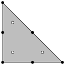
$\times$

$=$

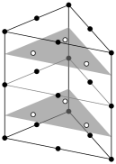
Figure 1. Second order triangular prism element and quadrature points. Black balls denote point evaluation nodes, and white balls mark quadrature points. The element and the quadrature rule are both tensor products of triangular and interval elements and quadrature rules respectively. Consequently, the tabulation matrix of the prism element is the Kronecker product of the tabulation matrices of the triangular and interval elements.

2.5. Collocated quadrature points

Spectral elements (Karniadakis and Sherwin, 2013; Patera, 1984) use Lagrange polynomials whose nodes are collocated with quadrature points. Typically, Gauss–Lobatto–Legendre (GLL) quadrature points are chosen for (continuous) interval elements, while Gauss–Legendre (GL) quadrature points are better for discontinuous elements. When these nodes match the quadrature rule that is used to approximate the integral, then the tabulation matrix becomes the identity matrix. In other words, FInAT can return

(2.12) $$\Psi_{i}(\xi_{q})\mapsto\delta_{iq},$$

and then the form compiler can optimise this away with a resulting simplification of the loop nests.

Another advantage of spectral elements is that they result in a better condition number of the assembled linear system than equidistant Lagrange elements, especially for higher polynomial degrees. We have added GaussLobattoLegendre and GaussLegendre elements to FIAT, and the appropriate element wrappers in FInAT. These wrappers are similar to the generic wrapper in section 2.2, except that they symbolically recognise if the tabulation points match the element nodes, in which case they replace the zeroth derivative according to eq. 2.12. GLL and GL are defined as one-dimensional quadrature rules, and they do not directly generalise to simplices. However, using tensor product elements one can construct higher-dimensional equivalents on box cells such as quadrilaterals and hexahedra.

2.6. Enriched element

By enriched element we mean the direct sum two (or more) finite elements. A basis for such an element is given by the concatenation of the bases of the summands. Let $V_{1}$ and $V_{2}$ be finite elements on the reference cell $K$, and let $\{\Psi^{(1)}_{i_{1}}\}_{i_{1}=1}^{N_{f,1}}$ and $\{\Psi^{(2)}_{i_{2}}\}_{i_{2}=1}^{N_{f,2}}$ be their bases respectively. The enriched element $V:=V_{1}\oplus V_{2}$ has basis $\{\Psi_{i}\}_{i=1}^{N_{f,1}+N_{f,2}}$ such that

(2.13) $$\Psi_{i}=\begin{cases}\Psi^{(1)}_{i}&\quad\mbox{when }1\leq i\leq N_{f,1},\\ \Psi^{(2)}_{i-N_{f,1}}&\quad\mbox{when }N_{f,1}<i\leq N_{f,1}+N_{f,2}.\end{cases}$$

For example, the triangular Mini element $P_{2}\oplus B_{3}$ denotes the space of quadratic polynomials enriched by a cubic “bubble” function (Arnold et al., 1984).

To implement this element, we utilise the newly introduced Concatenate node of GEM, which flattens the shape of its operands and concatenates them. For example, let $a$ be a $2\times 2$ matrix, $b$ a scalar, and $c$ a vector of length 3. Then $\mathtt{Concatenate}(a,b,c)$ is a vector of length 8 such that its first four entries correspond to the entries of $a$, its fifth entry to $b$, and its last three entries to $c$. We use this node to concatenate the basis functions of the subelements.

Let $\mathcal{E}^{(1)}_{i_{1}q}$ and $\mathcal{E}^{(2)}_{i_{2}q}$ denote the tabulation expressions for subelements $V_{1}$ and $V_{2}$. To correctly use Concatenate, basis function indices must become shape first, so the tabulation of $V$ is

(2.14) $${\mathtt{Concatenate}\left({\big{]}\mathcal{E}^{(1)}_{i_{1}q}\big{[}}_{i_{1}},{\big{]}\mathcal{E}^{(2)}_{i_{2}q}\big{[}}_{i_{2}}\right)}_{i}.$$

In the general case, any of $q$, $i_{1}$, and $i_{2}$ can be a multi-index. Moreover, enriched elements are not limited to scalar-valued finite elements, however, all subelements must have the same value shape. With value multi-index $\kappa$, eq. 2.14 generalises to

(2.15) $${\mathtt{Concatenate}\left({\big{]}\mathcal{E}^{(1)}_{i_{1}q\kappa}\big{[}}_{i_{1}},{\big{]}\mathcal{E}^{(2)}_{i_{2}q\kappa}\big{[}}_{i_{2}}\right)}_{i}.$$

Note that $q$ and $\kappa$ just pass through as free multi-indices, and only the basis function multi-indices $i_{1}$ and $i_{2}$ are replaced by the unified index $i$. We later show how enriched elements are destructured in the form compiler to recover the structure within the subelements.

2.7. Value modifier element wrappers

The facilities of FInAT for tensor product and enriched elements allow us to implement $H(\mathrm{div})$ and $H(\mathrm{curl})$ elements in a structure-revealing way. These elements are important in stable mixed finite element discretisations. Firedrake supports the whole $\mathcal{Q}^{-}$ family of the Periodic Table of the Finite Elements (Arnold and Logg, 2014). This family is defined on cube cells, and its members can be constructed out of interval elements. The continuous Q and the discontinuous dQ elements are just tensor products of interval elements, while the construction of $H(\mathrm{div})$ and $H(\mathrm{curl})$ conforming elements is slightly more complicated. McRae et al. (2016) provide constructions for $H(\mathrm{div})$ and $H(\mathrm{curl})$ elements. For example quadilateral Raviart-Thomas (1977) (RTCF) elements can be constructed as

(2.16) $$\mathrm{RTCF}_{n}=\mathtt{HDiv}(\mathrm{P}_{n}\otimes\mathrm{dP}_{n-1})\oplus\mathtt{HDiv}(\mathrm{dP}_{n-1}\otimes\mathrm{P}_{n})$$

where $\otimes$ denotes tensor product, $\oplus$ implies an enriched element, and $\mathtt{HDiv}$ is a special element wrapper that applies a transformation to the values of the basis functions of a tensor product element. Concretely, if $\Psi_{i}(\hat{x})$ is a basis function of $\mathrm{P}_{n}\otimes\mathrm{dP}_{n-1}$, then the corresponding basis function of $\mathtt{HDiv}(\mathrm{P}_{n}\otimes\mathrm{dP}_{n-1})$ is

(2.17) $$\Psi^{*}_{i}(\hat{x})=\begin{bmatrix}-\Psi_{i}(\hat{x})\\ 0\end{bmatrix}.$$

Note that $\Psi_{i}$ is a scalar-valued function, while $\Psi^{*}_{i}$ is a vector field. If $\mathtt{HDiv}$ is applied to $\mathrm{dP}_{n-1}\otimes\mathrm{P}_{n}$, then

(2.18) $$\Psi^{*}_{i}(\hat{x})=\begin{bmatrix}0\\ \Psi_{i}(\hat{x})\end{bmatrix}.$$

This difference may seem surprising, but it is possible because $\mathtt{HDiv}$ is defined as a long switch-case: based on the continuity and occasionally the reference value transformation of each factor element, it applies the transformation that makes the result suitable for building an $H(\mathrm{div})$ conforming element. $\mathtt{HCurl}$ behaves similarly for building $H(\mathrm{curl})$ conforming elements.

We have listed only two cases of $\mathtt{HDiv}$ in eqs. 2.17 and 2.18. For all cases of $\mathtt{HDiv}$ and $\mathtt{HCurl}$, as well as for a complete description of the construction of $\mathcal{Q}^{-}$ family elements, we refer to McRae et al. (2016). What is important at the moment, is that these element wrappers

• do not change or destroy the structure of the element they are applied to. (In the general case, $i$ is a multi-index.)

• allow us to build the $H(\mathrm{div})$ and $H(\mathrm{curl})$ conforming elements of the $\mathcal{Q}^{-}$ family, together with tensor product and enriched elements.

3. Form compiler algorithms

Expressing the inherent structure of finite elements is necessary, but not sufficient for achieving optimal code generation. The other main ingredient is algorithms for rearranging tensor contractions (called IndexSum in UFL and GEM) such that an optimal assembly algorithm is achieved.

These algorithms were implemented in the Two-Stage Form Compiler (TSFC) (Homolya et al., 2017), the form compiler used in Firedrake. In the first stage, TSFC lowers the finite element objects and geometric terms in weak form, and produces a tensor algebra expression in GEM. In the second stage, efficient C code is generated for the evaluation of GEM expression.

TSFC originally used FIAT for an implementation of finite elements, however changes have been made to the first stage to use FInAT instead. Since FInAT provides tabulations as GEM expressions, they integrate seamlessly into the intermediate representation of TSFC. The algorithms that rearrange tensor contractions were implemented as GEM-to-GEM transformers. The second stage has been largely left intact.

3.1. Delta cancellation: simple case

One important application of delta cancellation, by which we mean the simplification of loop nests involving Kronecker deltas, is found in our handling of mesh coordinates. The coordinate field is often stored in numerical software by assigning coordinates to each vertex of the mesh. This is equivalent to a vector-$P_{1}$ or vector-$Q_{1}$ finite element space. In fact, Firedrake represents coordinates as an ordinary finite element field, which facilitates support for higher-order geometries.

Since integral scaling involves the Jacobian of the coordinate transformation, virtually every finite element kernel is parametrised by this vector field. We have seen in section 2.3 that the FInAT implementation of vector elements contains Kronecker delta nodes; we now show how to simplify them away.

Consider a single entry $J_{ab}$ of the Jacobian matrix. We need its evaluation at each quadrature point $\xi_{q}$, let us call this $j_{q}:=J_{ab}(\xi_{q})$. Let $\{\Phi_{i}\}_{i=1}^{N_{c}}$ be the basis functions of the coordinate element, and let $\{c_{i}\}_{i=1}^{N_{c}}$ denote the local coefficients of this basis, so

(3.1) $$j_{q}:=J_{ab}(\xi_{q})=\sum_{i=1}^{N_{c}}c_{i}{\left[\frac{\partial\Phi_{i}}{\partial\hat{x}_{b}}(\xi_{q})\right]}_{a}.$$

Suppose we have a vector-$P_{2}$ coordinate element, then FInAT gives:

(3.2) $${\left[\frac{\partial\Phi_{i}}{\partial\hat{x}_{b}}(\xi_{q})\right]}_{a}\mapsto\mathbf{\Phi}^{(b,*)}_{i_{1}q}\delta_{i_{2}a}$$

where $i=(i_{1},i_{2})$ and $\mathbf{\Phi}^{(b,*)}$ is the tabulation expression of the $b$-th derivative of the scalar $P_{2}$ element. Applying the substitution yields:

(3.3) $$j_{q}=\sum_{i_{1},i_{2}}c_{(i_{1},i_{2})}\mathbf{\Phi}^{(b,*)}_{i_{1}q}\delta_{i_{2}a}.$$

Then the tensor product is disassembled into

• factors: $c_{(i_{1},i_{2})}$, $\mathbf{\Phi}^{(b,*)}_{i_{1}q}$, $\delta_{i_{2}a}$; and

• contraction indices: $i_{1}$, $i_{2}$.

Delta cancellation is carried out in this disassembled form. If there are any factors $\delta_{jk}$ or $\delta_{kj}$ such that $j$ is a contraction index, that factor is removed along with the contraction index $j$, and a $j\mapsto k$ index substitution is applied to all the remaining factors. This is repeated as long as applicable, and the repetition trivially terminates at latest when running out of contraction indices or delta factors.

This cancellation step is only applicable once to the example above, and it leaves us with factors $c_{(i_{1},a)}$ and $\mathbf{\Phi}^{(b,*)}_{i_{1}q}$ as well as contraction index $i_{1}$. Therefore, the optimised tensor product becomes

(3.4) $$j_{q}=\sum_{i_{1}}c_{(i_{1},a)}\mathbf{\Phi}^{(b,*)}_{i_{1}q}.$$

As one can see, this only needs the tabulation matrix of the scalar element, and each entry of the Jacobian only uses the relevant section of the array $c$.

3.2. Sum factorisation: Laplace operator

Sum factorisation is a well-known technique first proposed by Orszag (1980) that drastically reduces the algorithmic complexity of finite element assembly for high-order discretisations. To demonstrate this technique, consider the Laplace operator as introduced in section 1.1, and let the reference cell $\hat{K}$ be a square. This simplifies our notation, although TSFC supports higher dimensions uniformly. During UFL preprocessing, matrix-vector multiplications and the inner product in eq. 1.9 are rewritten as

(3.5) $$A^{K}_{ij}=\sum_{q=1}^{N_{q}}w_{q}S_{q}\sum_{k=1}^{2}\left(\sum_{l=1}^{2}G_{qlk}\frac{\partial\Psi_{i}}{\partial\hat{x}_{l}}(\xi_{q})\right)\left(\sum_{m=1}^{2}G_{qmk}\frac{\partial\Psi_{j}}{\partial\hat{x}_{m}}(\xi_{q})\right).$$

To be able to demonstrate a more generic case, we expand the geometric sums:

(3.6) $$A^{K}_{ij}=\sum_{q=1}^{N_{q}}w_{q}S_{q}\left\{\left(G_{q11}\frac{\partial\Psi_{i}}{\partial\hat{x}_{1}}(\xi_{q})+G_{q21}\frac{\partial\Psi_{i}}{\partial\hat{x}_{2}}(\xi_{q})\right)\left(G_{q11}\frac{\partial\Psi_{j}}{\partial\hat{x}_{1}}(\xi_{q})+G_{q21}\frac{\partial\Psi_{j}}{\partial\hat{x}_{2}}(\xi_{q})\right)\right.$$

$$\left.+\left(G_{q12}\frac{\partial\Psi_{i}}{\partial\hat{x}_{1}}(\xi_{q})+G_{q22}\frac{\partial\Psi_{i}}{\partial\hat{x}_{2}}(\xi_{q})\right)\left(G_{q12}\frac{\partial\Psi_{j}}{\partial\hat{x}_{1}}(\xi_{q})+G_{q22}\frac{\partial\Psi_{j}}{\partial\hat{x}_{2}}(\xi_{q})\right)\right\}.$$

With a tensor product element and quadrature rule as introduced in eqs. 1.14 and 1.16, FInAT provides the substitutions

(3.7) $$\frac{\partial\Psi_{i}}{\partial\hat{x}_{1}}(\xi_{q}) \mapsto D\mathbf{\Psi}^{(1)}_{i_{1}q_{1}}\mathbf{\Psi}^{(2)}_{i_{2}q_{2}}\quad\text{and}$$

(3.8) $$\frac{\partial\Psi_{i}}{\partial\hat{x}_{2}}(\xi_{q}) \mapsto\mathbf{\Psi}^{(1)}_{i_{1}q_{1}}D\mathbf{\Psi}^{(2)}_{i_{2}q_{2}}$$

where $i=(i_{1},i_{2})$, and $\mathbf{\Psi}^{(1)}$ and $\mathbf{\Psi}^{(2)}$ are numerical tabulation matrices of the one-dimensional elements, while $D\mathbf{\Psi}^{(1)}$ and $D\mathbf{\Psi}^{(2)}$ are tabulations of the first derivative respectively. Thus eq. 3.6 becomes

(3.9) $$A^{K}_{(i_{1},i_{2})(j_{1},j_{2})}=\textstyle{\sum}_{q_{1},q_{2}}w^{(1)}_{q_{1}}w^{(2)}_{q_{2}}S_{q_{1}q_{2}} \left\{\left(G_{q_{1}q_{2}11}D\mathbf{\Psi}^{(1)}_{i_{1}q_{1}}\mathbf{\Psi}^{(2)}_{i_{2}q_{2}}+G_{q_{1}q_{2}21}\mathbf{\Psi}^{(1)}_{i_{1}q_{1}}D\mathbf{\Psi}^{(2)}_{i_{2}q_{2}}\right)\right.$$

$$\quad\left(G_{q_{1}q_{2}11}D\mathbf{\Psi}^{(1)}_{j_{1}q_{1}}\mathbf{\Psi}^{(2)}_{j_{2}q_{2}}+G_{q_{1}q_{2}21}\mathbf{\Psi}^{(1)}_{j_{1}q_{1}}D\mathbf{\Psi}^{(2)}_{j_{2}q_{2}}\right)$$

$$+\left(G_{q_{1}q_{2}12}D\mathbf{\Psi}^{(1)}_{i_{1}q_{1}}\mathbf{\Psi}^{(2)}_{i_{2}q_{2}}+G_{q_{1}q_{2}22}\mathbf{\Psi}^{(1)}_{i_{1}q_{1}}D\mathbf{\Psi}^{(2)}_{i_{2}q_{2}}\right)$$

$$\quad\left.\left(G_{q_{1}q_{2}12}D\mathbf{\Psi}^{(1)}_{j_{1}q_{1}}\mathbf{\Psi}^{(2)}_{j_{2}q_{2}}+G_{q_{1}q_{2}22}\mathbf{\Psi}^{(1)}_{j_{1}q_{1}}D\mathbf{\Psi}^{(2)}_{j_{2}q_{2}}\right)\right\}.$$

Now we reached the intermediate representation of TSFC: all finite element basis functions have been replaced with tensor algebra expressions. Before we can apply sum factorisation, we need to apply argument factorisation to eq. 3.9. Argument factorisation transforms the expression to a sum-of-products form, such that no factor in any product depends on more than one of the free indices of form expression. In the above example, the free indices are $i_{1}$, $i_{2}$, $j_{1}$, and $j_{2}$. Equation 3.9 after argument factorisation looks like

(3.10) $$A^{K}_{(i_{1},i_{2})(j_{1},j_{2})}=\textstyle{\sum}_{q_{1},q_{2}} \left\{D\mathbf{\Psi}^{(1)}_{i_{1}q_{1}}\mathbf{\Psi}^{(2)}_{i_{2}q_{2}}D\mathbf{\Psi}^{(1)}_{j_{1}q_{1}}\mathbf{\Psi}^{(2)}_{j_{2}q_{2}}P^{(1,1)}_{q_{1}q_{2}}\right.$$

$$\quad+D\mathbf{\Psi}^{(1)}_{i_{1}q_{1}}\mathbf{\Psi}^{(2)}_{i_{2}q_{2}}\mathbf{\Psi}^{(1)}_{j_{1}q_{1}}D\mathbf{\Psi}^{(2)}_{j_{2}q_{2}}P^{(1,2)}_{q_{1}q_{2}}$$

$$\quad+\mathbf{\Psi}^{(1)}_{i_{1}q_{1}}D\mathbf{\Psi}^{(2)}_{i_{2}q_{2}}D\mathbf{\Psi}^{(1)}_{j_{1}q_{1}}\mathbf{\Psi}^{(2)}_{j_{2}q_{2}}P^{(2,1)}_{q_{1}q_{2}}$$

$$\quad\left.+\mathbf{\Psi}^{(1)}_{i_{1}q_{1}}D\mathbf{\Psi}^{(2)}_{i_{2}q_{2}}\mathbf{\Psi}^{(1)}_{j_{1}q_{1}}D\mathbf{\Psi}^{(2)}_{j_{2}q_{2}}P^{(2,2)}_{q_{1}q_{2}}\right\}$$

where $P^{(1,1)}_{q_{1}q_{2}}$, $P^{(1,2)}_{q_{1}q_{2}}$, $P^{(2,1)}_{q_{1}q_{2}}$, and $P^{(2,2)}_{q_{1}q_{2}}$ aggregate factors that do not depend on any of the free indices. Their precise definitions are:

(3.11a) $$P^{(1,1)}_{q_{1}q_{2}} :=w^{(1)}_{q_{1}}w^{(2)}_{q_{2}}S_{q_{1}q_{2}}(G_{q_{1}q_{2}11}G_{q_{1}q_{2}11}+G_{q_{1}q_{2}12}G_{q_{1}q_{2}12})$$

(3.11b) $$P^{(1,2)}_{q_{1}q_{2}} :=w^{(1)}_{q_{1}}w^{(2)}_{q_{2}}S_{q_{1}q_{2}}(G_{q_{1}q_{2}11}G_{q_{1}q_{2}12}+G_{q_{1}q_{2}12}G_{q_{1}q_{2}22})$$

(3.11c) $$P^{(2,1)}_{q_{1}q_{2}} :=w^{(1)}_{q_{1}}w^{(2)}_{q_{2}}S_{q_{1}q_{2}}(G_{q_{1}q_{2}11}G_{q_{1}q_{2}12}+G_{q_{1}q_{2}12}G_{q_{1}q_{2}22})$$

(3.11d) $$P^{(2,2)}_{q_{1}q_{2}} :=w^{(1)}_{q_{1}}w^{(2)}_{q_{2}}S_{q_{1}q_{2}}(G_{q_{1}q_{2}21}G_{q_{1}q_{2}21}+G_{q_{1}q_{2}22}G_{q_{1}q_{2}22})$$

Were there no restrictions on the factors, any expression would trivially be in a sum-of-products form. One can reach the argument factorised form through the mechanical application of the distributive property $a(b+c)\rightarrow ab+ac$ on products which have any factor with more than one free index. This rewriting always succeeds since the variational form is by definition linear in its arguments.

To continue with sum factorisation, let us concentrate on just one of the products for now. For example:

(3.12) $$\sum_{q_{1},q_{2}}D\mathbf{\Psi}^{(1)}_{i_{1}q_{1}}\mathbf{\Psi}^{(2)}_{i_{2}q_{2}}D\mathbf{\Psi}^{(1)}_{j_{1}q_{1}}\mathbf{\Psi}^{(2)}_{j_{2}q_{2}}P^{(1,1)}_{q_{1}q_{2}}$$

This requires $O(N_{q_{1}}N_{q_{2}}N_{f_{1}}N_{f_{2}}N_{f_{1}}N_{f_{2}})$ floating-point operations to evaluate. If the finite element is of polynomial order $n$ in both directions, then $N_{f_{1}}=N_{f_{2}}=n+1$, and also $N_{q_{1}}=N_{q_{2}}=O(n)$. This means $O(n^{6})$ operations. Rearranging eq. 3.12 as

(3.13) $$\sum_{q_{1}=1}^{N_{q_{2}}}D\mathbf{\Psi}^{(1)}_{i_{1}q_{1}}D\mathbf{\Psi}^{(1)}_{j_{1}q_{1}}\left(\sum_{q_{2}=1}^{N_{q_{2}}}\mathbf{\Psi}^{(2)}_{i_{2}q_{2}}\mathbf{\Psi}^{(2)}_{j_{2}q_{2}}P^{(1,1)}_{q_{1}q_{2}}\right)$$

only requires $O(N_{q_{1}}N_{q_{2}}N^{2}_{f_{2}}+N_{q_{1}}N^{2}_{f_{1}}N^{2}_{f_{2}})$ operations, and rearranging as

(3.14) $$\sum_{q_{2}=1}^{N_{q_{2}}}\mathbf{\Psi}^{(2)}_{i_{2}q_{2}}\mathbf{\Psi}^{(2)}_{j_{2}q_{2}}\left(\sum_{q_{1}=1}^{N_{q_{2}}}D\mathbf{\Psi}^{(1)}_{i_{1}q_{1}}D\mathbf{\Psi}^{(1)}_{j_{1}q_{1}}P^{(1,1)}_{q_{1}q_{2}}\right)$$

only requires $O(N_{q_{1}}N_{q_{2}}N^{2}_{f_{1}}+N_{q_{2}}N^{2}_{f_{1}}N^{2}_{f_{2}})$ operations. Both arrangements imply $O(n^{5})$ operations. Since the number of products in the argument factorised form only depends on the original weak form, but not on the polynomial order $n$, it is easy to see that assembling a bilinear form on a single quadrilateral requires $O(n^{6})$ operations naïvely, or $O(n^{5})$ operations with sum factorisation. Generally for a $d$-cube the operation count is $O(n^{3d})$ naïvely, and $O(n^{2d+1})$ with sum factorisation.

Finally, the only missing piece is a systematic algorithm that takes a tensor product such as eq. 3.12, and rearranges it into an optimal tensor product such as either eq. 3.13 or eq. 3.14. We first disassemble the tensor product into factors and contraction indices as in section 3.1, and then build an optimised tensor product from them. This problem has also been relevant in quantum chemistry applications, and is known as single-term optimisation in the literature. Lam et al. (1996) prove that this problem is NP-complete. Their algorithm explores combinations of factors to build a product tree, applying contractions on the way, and pruning the search tree to avoid traversing redundant expressions. Our approach, described in Algorithm 1, orders the contraction indices first: since we never have more than three of them, traversing all permutations is cheap.

1:function MakeTensorProduct($\mathtt{factors}$, $\mathtt{indices}$)

2:     $\mathtt{result}\leftarrow\mathit{nil}$

3:     $\mathtt{minops}\leftarrow\infty$

4:     for all $\mathtt{ordering}\in\textsc{Permutations}(\mathtt{indices})$ do

5:         $\mathtt{terms}\leftarrow\mathtt{factors}$

6:         $\mathtt{flops}\leftarrow 0$

7:         for $\mathtt{index}$ in $\mathtt{ordering}$ do $\triangleright$ apply contraction, one index at a time

8:              $\mathtt{contract}\leftarrow\{t\in\mathtt{terms}\mid\mathtt{index}\in\text{free indices of }t\}$

9:              $\mathtt{deferred}\leftarrow\{t\in\mathtt{terms}\mid\mathtt{index}\notin\text{free indices of }t\}$

10:

11:              $\mathtt{product},\mathtt{cost}\leftarrow\textsc{MakeProduct}(\mathtt{contract})$

12:              $\mathtt{term}\leftarrow$ IndexSum(product, (index,))

13:

14:              $\mathtt{terms}\leftarrow\mathtt{deferred}\cup\{\mathtt{term}\}$

15:              $\mathtt{flops}\leftarrow\mathtt{flops}+\mathtt{cost}+\prod_{i\in\text{free indices of }\mathtt{product}}i\mathtt{.extent}$

16:         end for

17:         $\mathtt{expr},\mathtt{cost}\leftarrow\textsc{MakeProduct}(\mathtt{terms})$

18:         $\mathtt{flops}\leftarrow\mathtt{flops}+\mathtt{cost}$

19:

20:         if $\mathtt{flops}<\mathtt{minops}$ then

21:              $\mathtt{result}\leftarrow\mathtt{expr}$

22:              $\mathtt{minops}\leftarrow\mathtt{flops}$

23:         end if

24:     end for

25:     return $\mathtt{result}$

26:end function

Algorithm 1 Building an optimal tensor product

The construction of an optimised tensor product expression happens in 5 to 18 of Algorithm 1. We apply contractions one index at a time. For example, let us contract along $q_{1}$ first. Then the set of factors are split based on dependence on $q_{1}$ (8 and 9). The factors in deferred are “pulled out” of $\sum_{q_{1}}$, while a product expression is constructed from the factors in contract using MakeProduct, followed by contraction over $q_{1}$. MakeProduct is a utility function for building a product expression tree from a set of factors, also returning the number of multiplications required to evaluate that product. For further gains, this function may associate factors in a optimised way, but for sum factorisation a trivial product builder suffices. For our example

(3.15) $$\mathtt{deferred} =\{\mathbf{\Psi}^{(2)}_{i_{2}q_{2}},\mathbf{\Psi}^{(2)}_{j_{2}q_{2}}\}\qquad\text{and}$$

(3.16) $$\mathtt{term} =\sum_{q_{1}}D\mathbf{\Psi}^{(1)}_{i_{1}q_{1}}D\mathbf{\Psi}^{(1)}_{j_{1}q_{1}}P^{(1,1)}_{q_{1}q_{2}}.$$

The new tensor contraction expression (term) is added to the deferred factors to produce the set of factors (terms) for the next iteration (14). In the next iteration we contract over $q_{2}$ and finally get eq. 3.14. For generality, we also handle the case in 17 to 18 when multiple factors remain after applying all contraction indices. This construction is repeated for each permutation of the contraction indices, and the expression requiring the lowest number of floating-point operations is selected. Looping over all permutations is not that bad, since $\left|\mathtt{indices}\right|\leq 3$ for all relevant problems.

3.3. Sum factorisation: parametrised forms

Partial differential equations are frequently parametrised by prescribed spatial functions, which are called coefficients in UFL. We have shown that matrix-free assembly of the operator action is analogous to assembling forms with coefficient functions, so as an example we now consider the action of the Laplace operator. We continue the description in section 1.1 from eq. 1.8, but now

(3.17) $$\hat{u}_{K}(\hat{x})=\sum_{i=1}^{N_{f}}U^{K}_{i}\Psi_{i}(\hat{x})$$

where $U^{K}\in\mathbb{R}^{N_{f}}$ is an array of local basis function coefficients. This results in

(3.18) $$b^{K}_{j}=\sum_{q=1}^{N_{q}}w_{q}S_{q}\left(G_{q}^{T}\sum_{i=1}^{N_{f}}U^{K}_{i}\hat{\nabla}\Psi_{i}(\xi_{q})\right)\cdot\left(G_{q}^{T}\hat{\nabla}\Psi_{j}(\xi_{q})\right)$$

where $b^{K}$ is the assembled local vector.

The common strategy is to first evaluate the coefficient function as $C_{q}\in\mathbb{R}^{d}$ at every quadrature point $q$, then simply use that in the form expression:

(3.19) $$C_{q} =\sum_{i=1}^{N_{f}}U^{K}_{i}\hat{\nabla}\Psi_{i}(\xi_{q})$$

(3.20) $$b^{K}_{j} =\sum_{q=1}^{N_{q}}w_{q}S_{q}(G_{q}^{T}C_{q})\cdot(G_{q}^{T}\hat{\nabla}\Psi_{j}(\xi_{q}))$$

The sum factorisation of eq. 3.20 is basically analogous to that which was shown in section 3.2. Equation 3.19 is even simpler: it is similar to the products of the argument factorised form, so it just needs disassembling and calling Algorithm 1.

Table 1 summarises the gains of sum factorisation considering various cell types, both for bilinear forms (matrix assembly) as well as for linear forms such as matrix-free operator actions or right-hand side assembly.

Table 1. Algorithmic complexity of form assembly on a single cell as a function of polynomial degree $n$.

Cell type	Linear form	Bilinear form
quadrilateral	$O(n^{4})$	$O(n^{6})$
triangular prism	$O(n^{6})$	$O(n^{9})$
hexahedron	$O(n^{6})$	$O(n^{9})$

(a) Naïve implementation

Cell type	Linear form	Bilinear form
quadrilateral	$O(n^{3})$	$O(n^{5})$
triangular prism	$O(n^{5})$	$O(n^{7})$
hexahedron	$O(n^{4})$	$O(n^{7})$

(b) Sum factorised implementation

3.4. Delta cancellation: nonzero patterns

In section 3.1, we considered delta cancellation for a common, but simple case; now we explore delta cancellation further. Previously, we could assume that the assembled local tensors were dense; now we are going to see that Kronecker delta nodes may cause particular nonzero patterns to appear.

For a concrete example, consider the vector mass form

(3.21) $$\int_{\Omega}u\cdot v\,\mathrm{d}x$$

where the trial function $u$ and the test function $v$ are chosen from vector-$P_{n}$ elements. Going through the usual steps, the integral on cell $K$ is evaluated as

(3.22) $$A^{K}_{ij}=\sum_{q=1}^{N_{q}}w_{q}S_{q}\Psi_{i}(\xi_{q})\cdot\Psi_{j}(\xi_{q}).$$

Recall that the usual translation of vector-$P_{n}$ elements is

(3.23) $${\left[\Psi_{i}(\xi_{q})\right]}_{k}\mapsto\mathbf{\Psi}^{*}_{i_{1}q}\delta_{i_{2}k}$$

where $i=(i_{1},i_{2})$ and $\mathbf{\Psi}^{*}$ is the tabulation matrix of the scalar $P_{n}$ element. Applying the substitution and rewriting the dot product we have

(3.24) $$A^{K}_{(i_{1},i_{2})(j_{1},j_{2})}=\sum_{q=1}^{N_{q}}w_{q}S_{q}\sum_{k=1}^{d}\mathbf{\Psi}^{*}_{i_{1}q}\delta_{i_{2}k}\mathbf{\Psi}^{*}_{j_{1}q}\delta_{j_{2}k}.$$

If we apply delta cancellation as described in section 3.1 to this product, we obtain

(3.25) $$A^{K}_{(i_{1},i_{2})(j_{1},j_{2})}=\sum_{q=1}^{N_{q}}w_{q}S_{q}\mathbf{\Psi}^{*}_{i_{1}q}\mathbf{\Psi}^{*}_{j_{1}q}\delta_{i_{2}j_{2}},$$

or if we build the tensor product with sum factorisation, even

(3.26) $$A^{K}_{(i_{1},i_{2})(j_{1},j_{2})}=\delta_{i_{2}j_{2}}\sum_{q=1}^{N_{q}}w_{q}S_{q}\mathbf{\Psi}^{*}_{i_{1}q}\mathbf{\Psi}^{*}_{j_{1}q}.$$

It is clear that $A^{K}$ has a particular nonzero pattern, that is $A^{K}_{(i_{1},i_{2})(j_{1},j_{2})}\neq 0$ only if $i_{2}=j_{2}$. To exploit this property, we need another delta cancellation step that operates across the assignment. That is, the tensor product is disassembled and deltas cancelled with contraction indices as in section 3.1. Then, still in the disassembled form, if there are any factors $\delta_{jk}$ or $\delta_{kj}$ such that $j$ is a free index of the return variable, then that factor is removed and a $j\mapsto k$ index substitution is applied to all the remaining factors as well as the return variable. Again, this is repeated as long as applicable. Finally, the tensor product is rebuilt.

In the example above, the return variable is $A^{K}_{(i_{1},i_{2})(j_{1},j_{2})}$, and its free indices are $i_{1}$, $i_{2}$, $j_{1}$, and $j_{2}$. Cancelling the remaining $\delta_{i_{2}j_{2}}$, we end up with

(3.27) $$A^{K}_{(i_{1},i_{2})(j_{1},i_{2})}=\sum_{q=1}^{N_{q}}w_{q}S_{q}\mathbf{\Psi}^{*}_{i_{1}q}\mathbf{\Psi}^{*}_{j_{1}q}.$$

Note the change in indexing the left-hand side.

In the general case, however, we will not have a nice product structure as in eq. 3.24. Nevertheless, if we apply argument factorisation as in section 3.2, then delta cancellation as described above can be applied to each product. Note that applying delta cancellation across assignments may cause different parts of the form expression to be “assigned” to different views of the return variable. A simple approach to correctly handle this case is to assume that the buffer holding $A^{K}$ is cleared at the beginning, and then make each “assignment” add to that buffer.

3.5. Splitting Concatenate nodes

Finally, we consider Concatenate nodes which come from enriched elements, and are crucial for the $H(\mathrm{div})$ and $H(\mathrm{curl})$ conforming elements of the $\mathcal{Q}^{-}$ family. For the sake of this discussion, we use the $\mathrm{RTCF}_{2}$ element as an example. As a corollary of eq. 2.16, this element is built as

(3.28) $$\mathrm{RTCF}_{2}=\mathtt{HDiv}(\mathrm{P}_{2}\otimes\mathrm{dP}_{1})\oplus\mathtt{HDiv}(\mathrm{dP}_{1}\otimes\mathrm{P}_{2}).$$

Its degrees of freedom consist of a $3\times 2$ matrix for $\mathrm{P}_{2}\otimes\mathrm{dP}_{1}$, and a $2\times 3$ matrix for $\mathrm{dP}_{1}\otimes\mathrm{P}_{2}$; a total of 12 degrees of freedom. This is graphically shown in Fig. 2.

Figure 2. Degrees of freedom of the $\mathrm{RTCF}_{2}$ element.

Suppose the quadrature rule is a tensor product rule with the same interval rule in both directions, then FInAT gives the tabulation expression:

(3.29) $${\mathtt{Concatenate}\left({\left]{(-\mathbf{\Psi}_{i_{1}q_{1}}\mathbf{\Phi}_{i_{2}q_{2}},0)}_{c}\right[}_{(i_{1},i_{2})},{\left]{(0,\mathbf{\Phi}_{i_{3}q_{1}}\mathbf{\Psi}_{i_{4}q_{2}})}_{c}\right[}_{(i_{3},i_{4})}\right)}_{I}$$

where

• $\mathbf{\Psi}$ and $\mathbf{\Phi}$ are the tabulation matrices of the $\mathrm{P}_{2}$ and $\mathrm{dP}_{1}$ interval elements respectively.

• $q_{1}$ and $q_{2}$ are quadrature indices with the same extent.

• $i_{1}$, $i_{2}$, $i_{3}$, and $i_{4}$ are basis function indices of the subelements.
  Their extents are 3, 2, 2, and 3 respectively.

• $c$ is the value index. ($\mathrm{RTCF}_{2}$ element is vector valued.)

• $I$ is the flat basis function index, with extent 12.

Suppose we have a buffer $b$ for the degrees of freedom, and that the above GEM expression is associated with the indexed buffer $b_{I}$. The principal approach to “implementing” Concatenate nodes is to split them in combination with the indexed buffer expression. Splitting eq. 3.29 with $b_{I}$ gives the following pairs:

(3.30) $$b_{i_{2}+2(i_{1}-1)}: \quad{(-\mathbf{\Psi}_{i_{1}q_{1}}\mathbf{\Phi}_{i_{2}q_{2}},0)}_{c}$$

(3.31) $$b_{6+i_{4}+3(i_{3}-1)}: \quad{(0,\mathbf{\Phi}_{i_{3}q_{1}}\mathbf{\Psi}_{i_{4}q_{2}})}_{c}$$

where $b_{i_{2}+2(i_{1}-1)}$ indexes the first 6 entries of $b$ as if it were $3\times 2$ matrix indexed by $(i_{1},i_{2})$, and $b_{6+i_{4}+3(i_{3}-1)}$ indexes the last 6 entries of $b$ as if it were $2\times 3$ matrix indexed by $(i_{3},i_{4})$. These indexed buffer expressions are easily generated: inspecting the shapes of the Concatenate node’s operands, we see which segment of $b$ corresponds to each operand and how that should be “reshaped”.

First, we discuss the splitting of Concatenate nodes which originate from the translation of trial and test functions. Suppose we have a bilinear form such as $\int_{\Omega}(\nabla\times u)\cdot(\nabla\times v)\,\mathrm{d}x$. Following the transformation to reference space, the assignment to the local tensor $A^{K}$ can be written as

(3.32) $$A^{K}_{I,J}:=\mathcal{F}\left(\Psi_{I},\hat{\nabla}\Psi_{I},\Psi_{J},\hat{\nabla}\Psi_{J}\right)\qquad 1\leq I\leq N_{f}\text{ and }1\leq J\leq N_{f}$$

where $\{\Psi_{I}\}_{I=1}^{N_{f}}$ is the basis of a finite element, $I$ and $J$ are basis function indices, and $\mathcal{F}$ is a functional. Sometimes generality may require second and further derivatives. Suppose the $\mathrm{RTCF}_{2}$ element was chosen as above, so $N_{f}=12$. Similarly, let $\{\Psi^{\textsc{x}}_{i_{1}i_{2}}\}_{(i_{1},i_{2})}$ be the basis of $\mathtt{HDiv}(\mathrm{P}_{2}\otimes\mathrm{dP}_{1})$ and $\{\Psi^{\textsc{y}}_{i_{3}i_{4}}\}_{(i_{3},i_{4})}$ be the basis of $\mathtt{HDiv}(\mathrm{dP}_{1}\otimes\mathrm{P}_{2})$. Note that

(3.33) $$\{\Psi^{\textsc{x}}_{i_{1}i_{2}}\}_{(i_{1},i_{2})} =\{\Psi_{I}\}_{I=1}^{6}\quad\text{and}$$

(3.34) $$\{\Psi^{\textsc{y}}_{i_{3}i_{4}}\}_{(i_{3},i_{4})} =\{\Psi_{I}\}_{I=7}^{12}.$$

Equation 3.32 can be trivially split into four assignments, for the combinations of ranges $1\leq I\leq 6$ and $7\leq I\leq 12$ with $1\leq J\leq 6$ and $7\leq J\leq 12$. Then the substitutions of eqs. 3.33 and 3.34 are directly applicable, which gives:

(3.35a) $$A^{K}_{i_{2}+2(i_{1}-1),\,j_{2}+2(j_{1}-1)} :=\mathcal{F}\left(\Psi^{\textsc{x}}_{i_{1}i_{2}},\hat{\nabla}\Psi^{\textsc{x}}_{i_{1}i_{2}},\Psi^{\textsc{x}}_{j_{1}j_{2}},\hat{\nabla}\Psi^{\textsc{x}}_{j_{1}j_{2}}\right)$$

(3.35b) $$A^{K}_{i_{2}+2(i_{1}-1),\,6+j_{4}+3(j_{3}-1)} :=\mathcal{F}\left(\Psi^{\textsc{x}}_{i_{1}i_{2}},\hat{\nabla}\Psi^{\textsc{x}}_{i_{1}i_{2}},\Psi^{\textsc{y}}_{j_{3}j_{4}},\hat{\nabla}\Psi^{\textsc{y}}_{j_{3}j_{4}}\right)$$

(3.35c) $$A^{K}_{6+i_{4}+3(i_{3}-1),\,j_{2}+2(j_{1}-1)} :=\mathcal{F}\left(\Psi^{\textsc{y}}_{i_{3}i_{4}},\hat{\nabla}\Psi^{\textsc{y}}_{i_{3}i_{4}},\Psi^{\textsc{x}}_{j_{1}j_{2}},\hat{\nabla}\Psi^{\textsc{x}}_{j_{1}j_{2}}\right)$$

(3.35d) $$A^{K}_{6+i_{4}+3(i_{3}-1),\,6+j_{4}+3(j_{3}-1)} :=\mathcal{F}\left(\Psi^{\textsc{y}}_{i_{3}i_{4}},\hat{\nabla}\Psi^{\textsc{y}}_{i_{3}i_{4}},\Psi^{\textsc{y}}_{j_{3}j_{4}},\hat{\nabla}\Psi^{\textsc{y}}_{j_{3}j_{4}}\right)$$

To be precise, TSFC does not inspect the construction of finite elements: this splitting of assignments is carried out at the GEM level, that is, after the substitution of basis function evaluations, thus TSFC only “sees” the occurrences of Concatenate nodes. This discussion, however, helps to demonstrate that the substitution of indexed Concatenate nodes such as eq. 3.29 with their split indexed expressions – like eqs. 3.30 and 3.31 – inside the intermediate form expression, along with the corresponding changes to indexing the result buffer, is a valid transformation that eliminates the Concatenate nodes and recovers any product structure within the subelements.

Lastly, we consider the evaluation of parametrising functions – also known as coefficients of the multilinear form – at quadrature points. Recalling eq. 3.17, we can apply a similar separation of basis functions and substitution, that is

(3.36) $$\hat{u}_{K}(\hat{x}) =\sum_{i=1}^{12}U^{K}_{i}\Psi_{i}(\hat{x})=\sum_{i=1}^{6}U^{K}_{i}\Psi_{i}(\hat{x})+\sum_{i=7}^{12}U^{K}_{i}\Psi_{i}(\hat{x})$$

(3.37) $$=\sum_{i_{1},i_{2}}U^{K}_{i_{2}+2(i_{1}-1)}\Psi^{\textsc{x}}_{i_{1}i_{2}}(\hat{x})+\sum_{i_{3},i_{4}}U^{K}_{6+i_{4}+3(i_{3}-1)}\Psi^{\textsc{y}}_{i_{3}i_{4}}(\hat{x}).$$

Having recovered the product structure, sum factorisation is now applicable to each summation separately. Again, we split Concatenate nodes along with indexed buffer expressions, but the latter now corresponds to an array of given numbers rather than the result buffer. Although the indexed Concatenate node is not necessarily outermost in the tabulation expression since the enriched element may not be outermost, this is not problem since all compound elements in section 2 are linear in their subelements.

3.6. Order of transformations

In previous subsections we have described a number of algorithms transforming the intermediate representation in TSFC. We finally list all transformations in the order of their application:

1. Split Concatenate nodes, see section 3.5.

2. Apply argument factorisation, see section 3.2.

3. Apply delta cancellation with tensor contractions, see section 3.1.

4. Apply delta cancellation across assignments, see section 3.4.

5. Apply sum factorisation, see section 3.2.
   Argument factorisation created a sum-of-products form, sum factorisation is applied on each product, but with the same ordering of contraction indices for all products, to leave more opportunities for factorisation based on the distributivity rule.

6. At each contraction level during sum factorisation: apply the ILP factorisation algorithm from COFFEE (Luporini et al., 2017). This factorisation is based on the distributivity rule, and especially improves bilinear forms (matrix assembly).

TSFC has several optimisation modes, which share the same UFL-to-GEM and GEM-to-C stages, but carry out different GEM-to-GEM transformations in between. Currently, TSFC offers the following modes:

• spectral mode applies all passes listed above. (The current default.)

• coffee mode implements a simplified version of the algorithm developed by Luporini et al. (2017). The simplification is that this mode unconditionally argument factorises, so it contains passes (1), (2), and (6). (The previous default.)

• vanilla mode aims to do as little as possible, so it only applies pass (1) since Concatenate nodes must be removed before the GEM-to-C stage. This mode corresponds to the original behaviour of TSFC described in Homolya et al. (2017) when most optimisations were done in COFFEE (Luporini et al., 2015; Luporini et al., 2017).

• tensor mode has two unique passes:

  1. Flatten Concatenate nodes, destroying their inner structure.

  2. Attempt to refactorise the integrand expression such that quadrature is pre-evaluated at compile time. This mimics the older tensor representation in FFC (Kirby and Logg, 2006, 2007), which is highly-performant for low-degree, constant-coefficient bilinear forms on affine simplices.

We must also note that modes have no effect on the evaluation of parametrising functions. For this purpose, we always apply passes (1) and (3), as well as sum factorisation according to section 3.3.

4. Evaluation

We now experimentally evaluate the performance benefits of this work, using the new spectral mode of TSFC with all FInAT elements. For comparison, we take a FIAT/coffee mode as baseline:

• Most FInAT elements are disabled, and instead we use the corresponding FIAT elements through the generic wrapper (section 2.2). Vector and tensor elements (section 2.3) are an exception: since we simplified the kernel interface with the FInAT transition, these elements have no direct equivalent in FIAT.

• The transformations of the coffee mode are applied. Kronecker delta nodes are replaced with indexing of an identity matrix.

We consider a range of polynomial degrees, and in most cases we plot the ratio of the number of degrees of freedom (DoFs) and execution time. This metric helps to compare the relative cost of different polynomial degrees.

The experiments were run on an workstation with two 2.6 GHz, 8-core E5-2640 v3 (Haswell) CPUs, for a total of 16 cores. The generated C kernels were compiled with -march=native -O3 -ffast-math using GCC 5.4.0 provided by Ubuntu 16.04.3 LTS.

4.1. Matrix assembly

To demonstrate delta cancellation, we first consider the Stokes momentum term

(4.1) $$\int_{\Omega}\nabla u:\nabla v\,\mathrm{d}x$$

where $u$ and $v$ are vector-valued trial and test functions respectively. To rule out the additional effects of sum factorisation, we evaluate this form on a tetrahedral mesh. Fig. 3 shows the difference in performance across a range of polynomial degrees, with more speed up for higher degrees. Note that for matrix assembly, if assembling an $N\times N$ sparse matrix takes $t$ seconds, then the DoFs/$s$ rate is $N/t$.

Figure 3. Stokes momentum term assembly on a tetrahedral mesh, excluding overheads like sparsity pattern creation and matrix initialisation.

Since some degrees of freedom are shared between cells, assembly needs to work on those DoFs multiple times. This effect reduces the DoFs/$s$ rate, and is stronger for low polynomial degrees. To approximately quantify this, we consider $Q_{n}$ elements: the number of unique degrees of freedom – neglecting boundary effects – is exactly $n^{d}$ per cell, while the number of degrees of freedom is $(n+1)^{d}$ for each cell. Suppose $O(n^{r})$ is the required number of floating-point operations per cell, where $r$ is the appropriate power. For low polynomial degrees, $c\cdot(n+1)^{r}$ with some constant $c$ is generally a closer approximation than $c\cdot n^{r}$. Therefore, assuming a degree-independent FLOPS rate, the DoFs/$s$ measure is approximated as

(4.2) $$C\cdot n^{d}/(n+1)^{r}.$$

Next, we consider the Laplace operator $\int_{\Omega}\nabla u\cdot\nabla v\,\mathrm{d}x$ on a hexahedral mesh to demonstrate sum factorisation. The expected per-cell algorithmic complexity is $O(n^{9})$ without and $O(n^{7})$ with sum factorisation, as anticipated in Table 1. Fig. 4 shows measurement data and confirms these expectations. We see orders of magnitude difference in performance for the highest degrees.

Figure 4. Number of degrees of freedom calculated per second for hexahedral Laplace operator assembly, excluding overheads like sparsity pattern creation and matrix initialisation.

We now demonstrate an interesting combination of delta cancellation and sum factorisation. Still considering the Laplace operator, we take the test and trial functions from a Gauss–Lobatto–Legendre finite element basis, and we consider a quadrature rule with collocated quadrature points (section 2.5). This quadrature rule is insufficient for exact integration, so the user has to specify the quadrature rule manually to enable this optimisation. This case appears in Fig. 4 as “underintegration”. However, the collocation enables FInAT to construct the substitution

(4.3) $$\frac{\partial\Psi_{i}}{\partial\hat{x}_{k}}(\xi_{q})\mapsto\begin{bmatrix}D\mathbf{\Psi}^{(1)}_{i_{1}q_{1}}\delta_{i_{2}q_{2}}\delta_{i_{3}q_{3}}\\ \delta_{i_{1}q_{1}}D\mathbf{\Psi}^{(2)}_{i_{2}q_{2}}\delta_{i_{3}q_{3}}\\ \delta_{i_{1}q_{1}}\delta_{i_{2}q_{2}}D\mathbf{\Psi}^{(3)}_{i_{3}q_{3}}\end{bmatrix}_{k}$$

where $i=(i_{1},i_{2},i_{3})$ and $q=(q_{1},q_{2},q_{3})$, and $D\mathbf{\Psi}^{(1)}$, $D\mathbf{\Psi}^{(2)}$, and $D\mathbf{\Psi}^{(3)}$ are tabulation matrices for the derivative of the interval elements. The algorithmic complexity of assembling the Laplace operator on nonaffine $d$-cubes could thus be reduced to $O(n^{d+2})$, while sum factorisation alone gets $O(n^{2d+1})$. Therefore, we would expect “underintegration” to approach $O(n^{5})$ on a hexahedral mesh, but in Fig. 4 it approaches $O(n^{6})$ instead, since global assembly in Firedrake still assumes a dense element stiffness matrix. However, analytically calculating the number of floating-point operations in the generated kernels, we can confirm that FInAT and TSFC optimise this case correctly (see Fig. 5).

Figure 5. Floating-point operations in generated kernels for hexahedral Laplace operator assembly.

Of course, the objective of this work is not simply to have another attempt at optimising the Laplace operator, but to have an automatic code generation system that can carry out these optimisations in principle on any form. As a more complicated example, we consider the simplest hyperelastic material model, the Saint Venant–Kirchhoff model (Logg et al., 2012, p. 529). First, we define the strain energy function over the displacement vector field $\mathbf{u}$:

(4.4) $$\mathbf{F} =\mathbf{I}+\nabla\mathbf{u} \triangleright\text{Deformation gradient}$$

(4.5) $$\mathbf{C} =\mathbf{F}^{T}\mathbf{F} \triangleright\text{Right Cauchy-Green tensor}$$

(4.6) $$\mathbf{E} =(\mathbf{C}-\mathbf{I})/2 \triangleright\text{Euler-Lagrange strain tensor}$$

(4.7) $$\Psi =\frac{\lambda}{2}[\operatorname{tr}(\mathbf{E})]^{2}+\mu\operatorname{tr}(\mathbf{E}^{2}) \triangleright\text{Strain energy function}$$

where $\lambda$ and $\mu$ are the Lamé parameters, and $\mathbf{I}$ is the identity matrix. Now, we define the Piola-Kirchhoff stress tensors:

(4.8) $$\mathbf{S} =\frac{\partial\Psi}{\partial\mathbf{E}} \triangleright\text{Second Piola-Kirchhoff stress tensor}$$

(4.9) $$\mathbf{P} =\mathbf{F}\mathbf{S} \triangleright\text{First Piola-Kirchhoff stress tensor}$$

UFL derives automatically that $\mathbf{S}=\lambda\operatorname{tr}(\mathbf{E})\mathbf{I}+2\mu\mathbf{E}$. Finally, the residual form of this nonlinear problem is

(4.10) $$r=\mathbf{P}:\nabla\mathbf{v}-\mathbf{b}\cdot\mathbf{v}$$

where $\mathbf{b}$ is the external forcing. To assemble a left-hand side, one must linearise the residual around an approximate solution $\mathbf{u}$:

(4.11) $$a=\delta r(\mathbf{u};\delta\mathbf{u})=\lim_{\epsilon\to 0}\frac{r(\mathbf{u}+\epsilon\delta\mathbf{u})-r(\mathbf{u})}{\epsilon}$$

This bilinear form has trial function $\delta\mathbf{u}$, test function $\mathbf{v}$, and $\mathbf{u}$ is a coefficient of the form. Fig. 6 plots the performance as a function of polynomial degree.

Figure 6. Number of degrees of freedom calculated per second for the left-hand side assembly of a hexahedral hyperelastic model, excluding overheads like sparsity pattern creation and matrix initialisation.

Finally, to demonstrate sum factorisation on $H(\mathrm{div})$ and $H(\mathrm{curl})$ conforming elements, we also consider the curl-curl operator, defined as

(4.12) $$a(u,v)=\int_{\Omega}(\nabla\times u)\cdot(\nabla\times v)\,\mathrm{d}x.$$

Here we use NCE elements, the hexahedral $H(\mathrm{curl})$ conforming element in the $\mathcal{Q}^{-}$ family. Fig. 7 shows that sum factorisation also works for this finite element with the spectral mode.

Figure 7. Number of degrees of freedom calculated per second for hexahedral curl-curl operator assembly, excluding overheads like sparsity pattern creation and matrix initialisation.

4.2. Operator action and linear forms

Since there are $O(n^{d})$ nonzero entries per row in the assembled matrix, $n$ being the polynomial order and $d$ the dimension, the matrix-free application of operator action is especially attractive for higher-order discretisations. The reasons are twofold. First, the memory requirement of storing the assembled matrix may be prohibitively expensive. In fact, this is the reason we only tested matrix assembly for degees up to 16. At that point, the size of the dense local tensor is 193MB, and we often need several temporaries of similar size, all of which are allocated on the stack. Even with unlimited stack size and just one cell plus halo region per core, we quickly run out of the available 64GB memory. Second, fast finite element assembly with sum factorisation will outperform matrix-vector multiplication with a pre-assembled sparse matrix, even if the cost of matrix assembly is ignored. This is because sparse matrix-vector multiplication takes $O(n^{2d})$ time per cell, while matrix-free assembly of operator action with sum factorisation only needs $O(n^{d+1})$.

We can directly compare sparse matrix-vector multiplication with various approaches to matrix-free algorithms using the metric of degrees of freedom per second, or DoFs/$s$. This is plotted for three configurations for calculating the action of the Laplace operator in Fig. 8, the left-hand side of a hyperelastic model in Fig. 9, and the curl-curl operator in Fig. 10.

Figure 8. Number of degrees of freedom calculated per second for hexahedral Laplace operator action.

Figure 9. Number of degrees of freedom calculated per second for the left-hand side action of a hexahedral hyperelastic model.

Figure 10. Number of degrees of freedom calculated per second for hexahedral curl-curl operator action.

Kirby and Mitchell (2017, §5.1) perform a similar comparison of matrix-free actions to assembled PETSc (Balay et al., 2017) matrices, but without access to sum factorisation. They find that:

1. Matrix-free applications are generally an $O(1)$ factor slower than matrix-vector products. When the Krylov subspace method runs no more than a few iterations, and the assembled matrix is not otherwise needed, then matrix-free applications could be overall cheaper the need for costly matrix assembly is eliminated.

2. For high polynomial orders, the memory requirement of the assembled matrix may simply be prohibitive.

Using sum factorised assembly, however, matrix-free applications are the clear fastest choice for high enough polynomial orders. For low orders, one must fall back to the considerations of point 1.

Note that $n^{3}/(n+1)^{4}$ initially increases before approaching $O(n^{-1})$ as $n\to\infty$, so the cost of sum factorised matrix-free application initially decreases with increasing polynomial order. The same applies for $n^{2}/(n+1)^{3}$ in 2D. As previously discussed, this is due to the decreasing portion of degrees of freedom that belong to multiple cells. At the same time, this effect renders sparse matrix-vector multiplication especially efficient at low polynomial orders, since the contributions of different cells are aggregated during matrix assembly.

We also observe that coffee mode does not outperform spectral mode even in case of low polynomial orders. This makes the latter a good default choice in TSFC for all cases. Furthermore, the use of FIAT elements was found to be infeasible in the high-order regime, because it resulted in kernels that are over 100MB both as C code and as executable binaries. Most of that size is occupied by tabulation matrices, which grow $O(n^{2d})$ in size, nevertheless GCC may not finish compiling them within an hour.

Finally, a note on form compilation time. Argument factorisation has a noticeable, but not prohibitive cost, while all other described transformations are cheap. A complicated hyperelastic model, the Holzapfel–Ogden model (Balaban et al., 2016) has been used for stress testing form compilers (Homolya et al., 2017, §6), since practical finite element models are seldom more difficult to compile. TSFC compiles its left-hand side in 1.4 seconds in vanilla mode, 5.6 seconds in coffee mode, and 5.9 seconds in spectral mode.

5. Conclusion and future work

We have presented a new, smarter library of finite elements, FInAT, which is able to express the structure inherent to some finite elements. We described the implemented FInAT elements, as well as the form compiler algorithms – which were implemented in TSFC – that exploit the exposed structure. With FInAT and TSFC, one can just write the weak form in UFL, and automatically get:

• sum factorisation with continuous, discontinuous, $H(\mathrm{div})$ and $H(\mathrm{curl})$ conforming elements on cuboid cells;

• optimised evaluation at collocated quadrature points with underintegration is requested; and

• minor optimisations with vector and tensor elements.

These techniques were known and have been applied in hand-written numerical software before, however, we are now able to utilise these optimisations in an automatic code generation setting in Firedrake.

This work is especially useful in combination with matrix-free methods (Kirby and Mitchell, 2017), enabling the development of efficient high-order numerical schemes while retaining high productivity. Our measurements show that on modern hardware one can increase the polynomial degree up to 8–10 without a notable increase in the run time of matrix-free operator applications (per degree of freedom).

Future work may include sum factorisation on simplicial cells, for example, through Bernstein polynomials (Ainsworth et al., 2011; Kirby and Thinh, 2012; Kirby, 2014b), as well as the evaluation and potentially optimisation of low-level performance on modern hardware.

Appendix A Code availability

For the sake of reproducibility, we have archived the specific versions of Firedrake components on Zenodo that were used for these measurements: PETSc (2017), petsc4py (2017), COFFEE (2017), PyOP2 (2017), FIAT (2017), FInAT (2017), UFL (2017), TSFC (2017a), and Firedrake (2017). For the FIAT/coffee mode, we applied a custom patch to TSFC (2017b). The experimentation framework is available at (Homolya, 2017).

References

- (1)
- Ainsworth et al. (2011) Mark Ainsworth, Gaelle Andriamaro, and Oleg Davydov. 2011. Bernstein–Bézier Finite Elements of Arbitrary Order and Optimal Assembly Procedures. SIAM Journal on Scientific Computing 33, 6 (2011), 3087–3109. https://doi.org/10.1137/11082539X
- Alnæs et al. (2015) Martin Sandve Alnæs, Jan Blechta, Johan Hake, August Johansson, Benjamin Kehlet, Anders Logg, Chris Richardson, Johannes Ring, Marie E. Rognes, and Garth N. Wells. 2015. The FEniCS Project Version 1.5. Archive of Numerical Software 3, 100 (2015), 9–23. https://doi.org/10.11588/ans.2015.100.20553
- Alnæs et al. (2014) Martin Sandve Alnæs, Anders Logg, Kristian B. Ølgaard, Marie E. Rognes, and Garth N. Wells. 2014. Unified Form Language: A Domain-Specific Language for Weak Formulations of Partial Differential Equations. ACM Trans. Math. Software 40, 2 (2014), 1–37. https://doi.org/10.1145/2566630 arXiv:1211.4047
- Arnold et al. (1984) Douglas N. Arnold, Franco Brezzi, and Michel Fortin. 1984. A stable finite element for the stokes equations. CALCOLO 21, 4 (01 Dec 1984), 337–344. https://doi.org/10.1007/BF02576171
- Arnold and Logg (2014) Douglas N. Arnold and Anders Logg. 2014. Periodic Table of the Finite Elements. SIAM News 47, 9 (November 2014), 212. https://femtable.org/
- Balaban et al. (2016) Gabriel Balaban, Martin S. Alnæs, Joakim Sundnes, and Marie E. Rognes. 2016. Adjoint multi-start-based estimation of cardiac hyperelastic material parameters using shear data. Biomechanics and Modeling in Mechanobiology 15, 6 (2016), 1509–1521. https://doi.org/10.1007/s10237-016-0780-7 arXiv:1603.03796
- Balay et al. (2017) Satish Balay, Shrirang Abhyankar, Mark F. Adams, Jed Brown, Peter Brune, Kris Buschelman, Lisandro Dalcin, Victor Eijkhout, William D. Gropp, Dinesh Kaushik, Matthew G. Knepley, Dave A. May, Lois Curfman McInnes, Karl Rupp, Patrick Sanan, Barry F. Smith, Stefano Zampini, Hong Zhang, and Hong Zhang. 2017. PETSc Users Manual. Technical Report ANL-95/11 - Revision 3.8. Argonne National Laboratory. http://www.mcs.anl.gov/petsc
- Bastian et al. (2014) Peter Bastian, Christian Engwer, Dominik Göddeke, Oleg Iliev, Olaf Ippisch, Mario Ohlberger, Stefan Turek, Jorrit Fahlke, Sven Kaulmann, Steffen Müthing, and Dirk Ribbrock. 2014. EXA-DUNE: Flexible PDE Solvers, Numerical Methods and Applications. In Euro-Par 2014: Parallel Processing Workshops (Lecture Notes in Computer Science), Luís Lopes, Julius Žilinskas, Alexandru Costan, Roberto G. Cascella, Gabor Kecskemeti, Emmanuel Jeannot, Mario Cannataro, Laura Ricci, Siegfried Benkner, Salvador Petit, Vittorio Scarano, José Gracia, Sascha Hunold, Stephen L Scott, Stefan Lankes, Christian Lengauer, Jesus Carretero, Jens Breitbart, and Michael Alexander (Eds.), Vol. 8806. Springer, Berlin, Heidelberg, 530–541. https://doi.org/10.1007/978-3-319-14313-2_45
- Cantwell et al. (2015) Chris D. Cantwell, David Moxey, A. Comerford, A. Bolis, G. Rocco, Gianmarco Mengaldo, Daniele De Grazia, S. Yakovlev, J. E. Lombard, D. Ekelschot, B. Jordi, H. Xu, Y. Mohamied, C. Eskilsson, B. Nelson, P. Vos, C. Biotto, R. M. Kirby, and S. J. Sherwin. 2015. Nektar++: An open-source spectral/hp element framework. Computer Physics Communications 192 (2015), 205–219. https://doi.org/10.1016/j.cpc.2015.02.008
- Fischer et al. (2008) Paul Fischer, J. Kruse, J. Mullen, H. Tufo, J. Lottes, and S. Kerkemeier. 2008. NEK5000: A fast and scalable open-source spectral element solver for CFD. (2008). Retrieved 27 October 2017 from https://nek5000.mcs.anl.gov
- Hecht (2012) Frédéric Hecht. 2012. New development in freefem++. Journal of Numerical Mathematics 20, 3-4 (2012), 251–266. https://doi.org/10.1515/jnum-2012-0013
- Hientzsch (2001) Bernhard Hientzsch. 2001. Fast Solvers and Domain Decomposition Preconditioners for Spectral Element Discretizations of Problems in H(curl). Ph.D. Dissertation. Courant Institute of Mathematical Sciences, New York University. http://www.cims.nyu.edu/~hientzsc/tr823l.pdf also Technical Report TR2001-823, December 2001, Department of Computer Science, Courant Institute.
- Homolya (2017) Miklós Homolya. 2017. Experimentation framework for manuscript “Exposing and exploiting structure: optimal code generation for high-order finite element methods,” version 1. (Nov. 2017). https://doi.org/10.5281/zenodo.1041785
- Homolya et al. (2017) Miklós Homolya, Lawrence Mitchell, Fabio Luporini, and David A. Ham. 2017. TSFC: a structure-preserving form compiler. (May 2017). arXiv:1705.03667v1 Submitted to SIAM Journal on Scientific Computing.
- Karniadakis and Sherwin (2013) George Karniadakis and Spencer Sherwin. 2013. Spectral/hp element methods for computational fluid dynamics. Oxford University Press.
- Kirby (2004) Robert C. Kirby. 2004. Algorithm 839: FIAT, A New Paradigm for Computing Finite Element Basis Functions. ACM Transactions on Mathematical Software (TOMS) 30, 4 (2004), 502–516. https://doi.org/10.1145/1039813.1039820
- Kirby (2014a) Robert C. Kirby. 2014a. High-Performance Evaluation of Finite Element Variational Forms via Commuting Diagrams and Duality. ACM Transactions on Mathematical Software (TOMS) 40, 4, Article 25 (July 2014), 24 pages. https://doi.org/10.1145/2559983
- Kirby (2014b) Robert C. Kirby. 2014b. Low-complexity finite element algorithms for the de Rham complex on simplices. SIAM Journal on Scientific Computing 36, 2 (2014), A846–A868. https://doi.org/10.1137/130927693
- Kirby and Logg (2006) Robert C. Kirby and Anders Logg. 2006. A compiler for variational forms. ACM Transactions on Mathematical Software (TOMS) 32, 3 (2006), 417–444. https://doi.org/10.1145/1163641.1163644 arXiv:1112.0402
- Kirby and Logg (2007) Robert C. Kirby and Anders Logg. 2007. Efficient Compilation of a Class of Variational Forms. ACM Transactions on Mathematical Software (TOMS) 33, 3, Article 17 (Aug. 2007). https://doi.org/10.1145/1268769.1268771 arXiv:1205.3014