Epi-two-dimensional fluid flow: a new topological paradigm for dimensionality

Abstract

While a variety of fundamental differences are known to separate two-dimensional (2D) and three-dimensional (3D) fluid flows, it is not well understood how they are related. Conventionally, dimensional reduction is justified by an a priori geometrical framework; i.e., 2D flows occur under some geometrical constraint such as shallowness. However, deeper inquiry into 3D flow often finds the presence of local 2D-like structures without such a constraint, where 2D-like behavior may be identified by the integrability of vortex lines or vanishing local helicity. Here we propose a new paradigm of flow structure by introducing an intermediate class, termed epi-2-dimensional flow, and thereby build a topological bridge between 2D and 3D flows. The epi-2D property is local, and is preserved in fluid elements obeying ideal (inviscid and barotropic) mechanics; a local epi-2D flow may be regarded as a ‘particle’ carrying a generalized enstrophy as its charge. A finite viscosity may cause ‘fusion’ of two epi-2D particles, generating helicity from their charges giving rise to 3D flow.

Phenomenologically, 2-dimensional (2D) fluid flow is very different from 3-dimensional (3D) flow in that the former is less-turbulent and more capable of generating and sustaining large-scale vortical structures Hasegawa1985 . This is because the dynamics of vortices in 2D systems is constrained, resulting in the suppression of some essential mechanisms of turbulence. Here we generalize by replacing the usual geometrical constraint by a topological constraint that extracts the essential property of 2D flow. We call such constrained flow epi-2D.

Conventionally, the 2D geometrical constraint is believed appropriate for a fluid with limited depth and slow variation of physical quantities in the vertical direction compared to those in the horizontal directions. However, 2D-like behavior, our epi-2D flow, may occur in flows without being strictly 2D. For example, sometimes in 3D systems, flow may not be totally 3D by having subdomains in which the flow is 2D-like CF1993 .

In this work we precisely formulate the concept of epi-2D flow. The difference in the invariants of 3D and 2D systems serves as a guide: as is well-known, the helicity is a constant of motion in an ideal 3D flow Moreau ; helicity , while in 2D geometry the helicity degenerates to zero, being compensated by the enstrophy (or its generalization as described below). Usually, these two different invariants are regarded as attributes of different dimensionality Fukumoto ; but, we switch the viewpoints and use the invariants as discriminants of dimensionality. Interestingly, the class of flows that conserve (appropriately generalized) enstrophy is much larger than the geometrical 2D class. This extended class is what we refer to as epi-2D. We will see that the ‘fusion’ of two epi-2D flows may yield a 3D flow, transmuting the corresponding enstrophies into helicity. In fact, the epi-2D behavior is a local property, so we can formulate a ‘particle picture’ of transmutation.

Consider first the basic equations and conservation laws of fluid mechanics. Let ${M}$ be a 3D domain containing an ideal (invicid) barotropic fluid. We assume ${M}=\mathbb{T}^{3}$, the 3-torus, and ignore boundary effects BC . Denoting by ${\rho}$ the mass density, $\bm{V}$ the fluid velocity, $P$ the pressure, the governing equations are

$$\partial_{t}{\rho}=-\nabla\cdot(\bm{V}{\rho}),$$ (1)

$$\partial_{t}\bm{V}=-(\bm{V}\cdot\nabla)\bm{V}-\nabla h,$$ (2)

where $\rho^{-1}\nabla P=\nabla h$ with an enthalpy $h=h(\rho)$, The energy of the system is

$$H=\int_{M}\left[\frac{1}{2}|\bm{V}|^{2}+\varepsilon(\rho)\right]\,\rho\,\mathrm{d}^{3}x,$$ (3)

where $\varepsilon(\rho)$ is the internal energy per unit mass and $\partial(\rho\epsilon)/\partial\rho=h$. It follows by direct calculation that the energy $H$, the helicity,

$$C=\int_{M}\bm{V}\cdot\bm{\omega}\,\mathrm{d}^{3}x,$$ (4)

with $\bm{\omega}=\nabla\times\bm{V}$ being the vorticity, and the total mass, $N=\int_{M}\rho\,\mathrm{d}^{3}x$, are conserved.

The 2D geometrical reduction can be obtained as follows. Let $z$ be a ‘perpendicular’ coordinate in the Cartesian $(x,y,z)$ system and let $\bm{e}_{z}=\nabla z$. The reduction with $\bm{e}_{z}\cdot\bm{V}=0$ and $\partial_{z}=0$ yields the 2D system on the $x$-$y$ plane (a flat torus $\mathbb{T}^{2}$). Using $\bm{V}=(v_{x},v_{y},0)^{\mathrm{T}}$ and $\bm{v}=(v_{x},v_{y})^{\mathrm{T}}$, the vorticity becomes $\bm{\omega}=\nabla\times\bm{V}=\omega\bm{e}_{z}$, where $\omega=\partial_{x}v_{y}-\partial_{y}v_{x}$. Because $\bm{V}\cdot\bm{\omega}=0$ for this 2D reduction, helicity conservation is now trivial: $C\equiv 0$. Interestingly, however, a different invariant emerges: the generalized enstrophy

$${Q}=\int_{M}f(\vartheta)\rho\,\mathrm{d}^{2}x,$$ (5)

with the potential vorticity $\vartheta=\omega/\rho$, is now a constant of motion ($f$ being an arbitrary smooth function). It is also easy to show the constancy of the ‘local’ enstrophy that is defined by replacing the domain $M$ of the integral (5) by an arbitrary co-moving (i.e. transported by the flow $\bm{v}$) sub-domain $\Sigma(t)$. For the simple choice $f(\vartheta)=\vartheta$, the local enstrophy reads ${Q}=\int_{\Sigma(t)}\omega\,\mathrm{d}^{2}x=\oint_{\partial\Sigma(t)}\bm{v}\cdot\,\mathrm{d}\bm{x}$, and the constancy of this $Q$ is known as Kelvin’s circulation theorem. For an incompressible flow ($\nabla\cdot\bm{v}=0$), we may assume $\rho=$ constant, and then $Q$ has a special form $\int\omega^{2}\,\mathrm{d}^{2}x$, which is the usual enstrophy.

Our formulation of epi-2D flow begins by inquiring into the root cause of these invariants, deemed as a reflection of some symmetry. In particular, we replace the geometrical symmetry $\bm{e}_{z}\cdot\,=0$ and $\partial_{z}=0$ that characterizes the 2D system by a gauge symmetry that yields an equivalent enstrophy invariant.

The fluid equations (1)–(2) are a Hamiltonian field theory on a phase space $\mathcal{V}$ of fluid variables $\bm{u}=(\rho,\bm{V})^{\textrm{T}}$ MG80 ; Morrison-RMP . The constancy of the Hamiltonian (energy) $H$ is due to $\partial_{t}H=0$. In contrast, the conservation of the total mass $N$ and the helicity $C$ is independent of the choice of Hamiltonian, implying that they are not related to any explicit symmetry of the system. Such constants of motion are called Casimir invariants. A possible mechanism that yields a Casimir invariant is a gauge symmetry in some representation of $\mathcal{V}$. If there is an underlying phase space $X$ of fundamental variables $\bm{\xi}$, with the physical variables $\bm{u}$ represented by some specific combinations of $\bm{\xi}$ where the map $\bm{\xi}\mapsto\bm{u}$ is redundant, then a gauge freedom occurs and a Casimir invariant is a Noether charge of the gauge symmetry. One example of this is the relabeling symmetry of the Lagrangian to Eulerian fluid representations pjmP96 , but for the purposes here the relevant symmetry is that of the Clebsch parameterization Clebsch ; pjmAIP ; Marsden1983 ; Yoshida2009 ; YM2016 , for which it was shown that $N$ and $C$ are Noether charges TanehashiYoshida2015 .

Let $X$ be the phase space of Clebsch parameters

$$\bm{\xi}=(\varrho,\varphi,p,q,r,s)^{\mathrm{T}}~{}\in X,$$ (6)

where each $\xi_{j}$ ($j=1,\cdots,6$) is a function on the base space ${M}=\mathbb{T}^{3}$ suppl1 . On the space of observables (i.e. smooth functionals on $X$), we define a canonical Poisson bracket

$$\{F,G\}=\langle\partial_{\bm{\xi}}F,J\partial_{\bm{\xi}}G\rangle,$$ (7)

where $\langle\bm{\eta},\bm{\xi}\rangle=\int_{M}\bm{\eta}\cdot\bm{\xi}\,\mathrm{d}^{3}x$, $\partial_{\bm{\xi}}F$ is the gradient of $F$ in $X$, and $J$ is the symplectic operator

$$J=J_{c}\oplus J_{c}\oplus J_{c},\quad J_{c}=\left(\begin{array}[]{cc}0&I\\ -I&0\end{array}\right).$$ (8)

Given a Hamiltonian $H$, the adjoint representation of Hamiltonian dynamics is ${\mathrm{d}}F/{\mathrm{d}t}=\{F,H\}$, which is equivalent to Hamilton’s equation of motion

$$\partial_{t}\bm{\xi}=J\partial_{\bm{\xi}}H.$$ (9)

We relate the physical quantity $\bm{u}\in\mathcal{V}$ and $\bm{\xi}\in X$ by $\rho\Leftrightarrow\varrho$ and (denoting $\check{p}={p}/{\varrho}$, and $\check{{r}}={{r}}/{\varrho}$)

$$\bm{V}\Leftrightarrow\bm{\wp}=\nabla\varphi+\check{p}\nabla q+\check{{r}}\nabla{s}.$$ (10)

Writing a vector as (33) is called the Clebsch parameterization Clebsch ; pjmAIP ; Marsden1983 . The five Clebsch parameters $(\varphi,\check{p},q,\check{r},s)$ are sufficient to represent every 3-vector (1-form in 3D space) Yoshida2009 . Inserting (33) into the fluid energy (3), we obtain the Hamiltonian

$$H(\bm{\xi})=\int_{M}\left[\frac{1}{2}{\left|\nabla\varphi+\frac{p}{\varrho}\nabla q+\frac{{r}}{\varrho}\nabla{s}\right|^{2}}+\varepsilon(\varrho)\right]\varrho\,\mathrm{d}^{3}x.$$ (11)

With this $H$, the equation of motion (9) reads BC

$$\left\{\begin{array}[]{l}\partial_{t}\varrho+\nabla\cdot(\bm{V}\varrho)=0,\\ \partial_{t}\varphi+\bm{V}\cdot\nabla\varphi=h-\frac{1}{2}{V^{2}},\\ \partial_{t}p+\nabla\cdot(\bm{V}p)=0,\quad\partial_{t}q+\bm{V}\cdot\nabla q=0,\\ \partial_{t}r+\nabla\cdot(\bm{V}r)=0,\quad\partial_{t}s+\bm{V}\cdot\nabla s=0.\end{array}\right.$$ (12)

The first equation of (36) is nothing but the mass conservation law (1). Evaluating $\partial_{t}\bm{V}$ by inserting (33) and using (36), we obtain (2). Hence, Hamilton’s equation (9) with the Hamiltonian (34) describes fluid motion obeying (1) and (2) Lin ; Zakharov ; pjmAIP . The invariance of the helicity $C$ also follows from (36).

We examine how the 2D geometrical reduction works in the Hamiltonian formalism. In a 2D system (${M}=\mathbb{T}^{2}$), we can parameterize a general 2D velocity as

$$\bm{V}\Leftrightarrow\bm{\wp}=\nabla\varphi+\check{p}\nabla q,\quad(\check{p}=p/\varrho).$$ (13)

Here, only three Clebsch parameters $\varphi$, $\check{p}$, and $q$ are sufficient Yoshida2009 . The vorticity is $\omega=(\nabla\check{p}\times\nabla q)\cdot\bm{e}_{z}$. The helicity cannot be defined in the 2D space. The potential vorticity is a scalar $\vartheta=\omega/\varrho$, and the generalized enstrophy reads $Q=\int_{\Sigma(t)}f(\omega/\varrho)\varrho\,\mathrm{d}^{2}x$, where a sub-domain $\Sigma(t)$ is moved by the group-action of $\mathrm{e}^{t\bm{v}}$. We can easily verify $\mathrm{d}Q/\mathrm{d}t=0$ by (36).

Epi-2D flow is obtained in the 3D setting with the phase space $X$ on the base space $M=\mathbb{T}^{3}$ by setting ${r}=0$ 2.5D . The corresponding physical fields are $\rho\Leftrightarrow\varrho$ and

$$\bm{V}\Leftrightarrow\bm{\wp}=\nabla\varphi+\check{p}\nabla q,\quad\left(\check{p}={p}/{\varrho}\right).$$ (14)

This yields a 2D-like representation, but there is a difference between (13) for 2D flow and (37) for epi-2D flow, for the latter resides in the 3D domain $\mathbb{T}^{3}$.

Epi-2D flow is generated by the reduced Hamiltonian

$$H(\bm{\xi})=\int_{M}\left[\frac{1}{2}{\left|\nabla\varphi+\frac{p}{\varrho}\nabla q\right|^{2}}+\varepsilon(\varrho)\right]\varrho\,\mathrm{d}^{3}x,$$ (15)

giving the 3D equations (1) and (2). While ${s}$ does not appear in (38), it obeys the same equation (36) but with $\bm{V}$ independent of ${s}$. Such a field, co-moving with the epi-2D flow, is called a phantom field YoshidaMorrisonFDR2014 . Or, $s$ is a gauge field with the observables blind to its initial value.

As previously remarked, (37) cannot represent an arbitrary 3D flow: epi-2D flow may have a finite vorticity $\bm{\omega}=\nabla\times\bm{\wp}=\nabla\check{p}\times\nabla q$, but its helicity density $\bm{\wp}\cdot(\nabla\times\bm{\wp})=\nabla\varphi\cdot(\nabla\check{p}\times\nabla q)=\nabla\cdot(\varphi\nabla\check{p}\times\nabla q)$ is an exact differential, implying zero helicity, $C=\int_{{M}}\bm{\wp}\cdot(\nabla\times\bm{\wp})\,\mathrm{d}^{3}x=0$.

As for 2D, this degeneracy of the helicity is compensated by a different invariant obtained by extending the generalized enstrophy to 3D. With the phantom $s$,

$${Q}:=\int_{\Omega(t)}f(\vartheta)\,\varrho\,\mathrm{d}^{3}x,\quad\vartheta=\frac{\bm{\omega}\cdot\nabla{s}}{\varrho},$$ (16)

with arbitrary $f$ and an arbitrary co-moving 3D volume element $\Omega(t)\subset{M}$, is seen to be conserved upon making use of (36). If we choose $s=z$, then (39) reduces to the 2D form $Q=\int_{\Sigma(t)}f(\omega/\varrho)\varrho\,\mathrm{d}^{2}x$. In what follows, we choose the simplest case $f(\vartheta)=\vartheta$.

Local epi-2D regions within a 3D flow can be exploited to define particle-like behavior. With the general 3D parameterization $\bm{V}\Leftrightarrow\bm{\wp}=\nabla\varphi+\check{p}\nabla q+\check{{r}}\nabla{s}$, a region in which $\check{{r}}=0$ may be called an epi-2D domain. Since $\check{{r}}$ co-moves with the fluid, every infinitesimal volume element, say $\Omega_{j}(t)$ with elements indexed by $j$, included in an epi-2D domain may be viewed as a quasiparticle, which we call an epi-2D particle. The generalized enstrophy evaluated for the vorticity $\bm{\omega}_{+}=\nabla\check{{p}}\times\nabla{q}$ in $\Omega_{j}(t)$, denoted by ${Q}_{+}(\Omega_{j})$, is a constant of motion. Here the index ‘+’ is used to distinguish from counterpart domains where $\check{p}=0$, for which ${Q}_{-}(\Omega_{j})=\int_{\Omega_{j}(t)}\vartheta_{-}\varrho\,\mathrm{d}^{3}x$, where $\vartheta_{-}=(\bm{\omega}_{-}\cdot\nabla q)/\varrho$ with the vorticity $\bm{\omega}_{-}=\nabla\check{{r}}\times\nabla{s}$.

We call ${Q}_{\pm}(\Omega_{j})$ the charge of the epi-2D particle $\Omega_{j}$. It is remarkable that both ${Q}_{+}$ and ${Q}_{-}$ are invariant even in 3D flows. Both charges essentially measure the ‘circulations’ of the decomposed components of the flow (cf. the comment following (5)). In fact, Kelvin’s circulation theorem applies in general 3D flows. The merit of the use of the charges $Q_{\pm}$, in comparison with the conventional circulation, is in that they can delineate the local flow structure. As far as a particle (volume element) carries only $Q_{+}$ or $Q_{-}$, it is epi-2D. However, when the vorticity is in a mixed state, i.e., $\bm{\omega}=\bm{\omega}_{+}+\bm{\omega}_{-}=\nabla\check{p}\times\nabla q+\nabla\check{{r}}\times\nabla{s}$, the particle becomes 3D, and then, helicity is created from the charges $Q_{+}$ and $Q_{-}$. Indeed, the integrands of $Q_{+}$ and $Q_{-}$ (the charge densities) are, respectively,

$$\mathscr{Q}_{+}=(\nabla\check{{p}}\times\nabla q)\cdot\nabla{s},\quad\mathscr{Q}_{-}=(\nabla\check{{r}}\times\nabla{s})\cdot\nabla q,$$

while the integrand of $C$ (the helicity density) is

$$\mathscr{C}=\bm{\wp}\cdot(\nabla\times\bm{\wp})=\check{{r}}\mathscr{Q}_{+}+\check{{p}}\mathscr{Q}_{-}+\mathscr{C}_{\textrm{ex}},$$ (17)

where $\mathscr{C}_{\textrm{ex}}=\nabla\varphi\cdot(\nabla\check{{p}}\times\nabla{q}+\nabla\check{{r}}\times\nabla{s})$ is the exact part of the helicity density. The residual helicity density $\mathscr{C}_{\mathrm{r}}=\mathscr{C}-\mathscr{C}_{\textrm{ex}}=\check{{r}}\mathscr{Q}_{+}+\check{{p}}\mathscr{Q}_{-}$ describes the coupling of epi-2D particles; evidently, either $\check{r}=0$ or $\check{p}=0$ causes $\mathscr{C}_{\mathrm{r}}$ to vanish. Conversely, the combination of two charges $\mathscr{Q}_{+}$ and $\mathscr{Q}_{-}$ yields $\mathscr{C}_{\mathrm{r}}$. Therefore, $\mathscr{C}_{\mathrm{r}}=0$ can be used as an alternative definition of epi-2D flow.

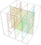
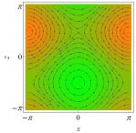
Figure 1: An epi-2D flow given by $\bm{V}_{+}$. (Left) The integrable vortex lines. (Right) Contours of $\mathscr{Q}_{+}$ and the flow vector on the surface $y=0$ indicated by the gray cross-section in the left figure (color code ranges from orange$=2$ to green$=-2$).

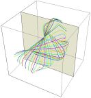
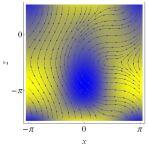
Figure 2: The combination $\bm{V}=\bm{V}_{+}+\bm{V}_{-}$ yields a 3D flow. (Left) The vortex lines become chaotic (non-integrable). (Right) Contours of $\mathscr{C}_{\mathrm{r}}$ together with the surface-aligned component of the flow vector on the surface $y=0$ indicated by the gray cross-section in the left figure (color code ranges from blue$=5$ to yellow$=-1$).

We give an illustrative example to visualize epi-2D flow and its transition to 3D. Let $(x,y,z)$ be Cartesian coordinates, and $\bm{V}=\alpha\bm{V}_{+}+\beta\bm{V}_{-}$ with

$$\bm{V}_{+}=\left(\begin{array}[]{c}b\sin y-c\cos z\\ 0\\ a\sin x\end{array}\right),~{}\bm{V}_{-}=\left(\begin{array}[]{c}0\\ c\sin z-a\cos x\\ -b\cos y\end{array}\right),$$

where $\alpha,\beta,a,b$ and $c$ are arbitrary real constants, and the vorticities satisfy $\bm{\omega}_{\pm}=\nabla\times\bm{V}_{\pm}=\bm{V}_{\mp}$. When $\alpha=\beta=1$, $\bm{V}$ is the famous ABC flow abc , satisfying $\nabla\times\bm{V}=\bm{V}$. We may cast $\bm{V}$ into the Clebsch form (33) with

$$\left\{\begin{array}[]{ll}\varphi=(\alpha a\sin x-\beta b\cos y)z,&{}\\ \check{p}=\alpha[b\sin y-c\cos z-(a\cos x)z],&q=x,\\ \check{{r}}=\beta[c\sin z-a\cos x-(b\sin y)z],&s=y.\end{array}\right.$$ (18)

When $\alpha=1$ and $\beta=0$, we obtain an epi-2D flow $\bm{V}_{+}$ with $\mathscr{Q}_{+}=c\sin z-a\cos x$. The co-presence of $\bm{V}_{+}$ and $\bm{V}_{-}$ creates a 3D flow; when $\alpha=\beta=1$, $\bm{V}$ has the residual helicity density $\mathscr{C}_{\mathrm{r}}={r}\mathscr{Q}_{+}+p\mathscr{Q}_{-}$. In Fig. 1, we show the structure of $\bm{V}_{+}$ and the distribution of $\mathscr{Q}_{+}$ on a surface $y=0$. Figure 2 depicts the 3D flow $\bm{V}=\bm{V}_{+}+\bm{V}_{-}$ and $\mathscr{C}_{\mathrm{r}}$ on a cross-section of $y=0$.

Table 1: Topological classification of flows. $\bm{V}$: 3D flow, $\bm{V}_{\mathrm{r}}=\bm{V}-\nabla\varphi$: solenoidal component, $\mathscr{Q}_{\pm}$: generalized enstrophy density, $Q_{\pm}=\int_{\Omega(t)}\mathscr{Q}_{\pm}\,\mathrm{d}^{3}x$: generalized enstrophy, $\mathscr{C}$: helicity density, $\mathscr{C}_{\mathrm{r}}$: residual helicity density, $C=\int_{M}\mathscr{C}_{\mathrm{r}}\,\mathrm{d}^{3}x$: helicity. Notice that the local integral $\int_{\Omega(t)}\mathscr{C}_{\mathrm{r}}\,\mathrm{d}^{3}x$ is not a constant of motion.

classification	representation	invariants
$\begin{array}[]{l}\textrm{vorticity-free}\\ (\nabla\times\bm{V}=0)\end{array}$	$\bm{V}=\nabla\varphi$	$\begin{array}[]{l}\mathscr{C}=0\\ \mathscr{Q}=0\end{array}$
$\begin{array}[]{l}\textrm{helicity-free}\\ (\bm{V}\cdot\nabla\times\bm{V}=0)\end{array}$	$\bm{V}=\check{p}\nabla q$	$\begin{array}[]{l}\mathscr{C}=0\\ {Q}_{\pm}\end{array}$
$\begin{array}[]{l}\textrm{epi-2D}\\ (\bm{V}_{\mathrm{r}}\cdot\nabla\times\bm{V}_{\mathrm{r}}=0)\end{array}$	$\bm{V}=\nabla\varphi+\check{p}\nabla q$	$\begin{array}[]{l}\mathscr{C}_{\mathrm{r}}=0\\ {Q}_{\pm}\end{array}$
general	$\bm{V}=\nabla\varphi+\check{p}\nabla q+\check{{r}}\nabla{s}$	$\begin{array}[]{l}C\\ {Q}_{\pm}\end{array}$

Table 2 summarizes our newly proposed classification of flows. The smallest set hosts vorticity-free, potential flow (or lamellar field lamellar ). The next of the hierarchy includes ‘weighted’ potential flows (or complex lamellar field) that have vorticity but still zero helicity density. A further generalization yields the epi-2D flows that have only exact helicity density (hence, $\mathscr{C}_{\mathrm{r}}=0$). The epi-2D class subsumes conventional 2D systems where we may take $s=z$ (the perpendicular coordinate); this is possible since $\bm{\omega}$ is aligned to the fixed vector $\bm{e}_{z}$ symmetries . As the generalization of the a priori base space of a 2D system, an epi-2D flow has intrinsic vortex surfaces (cf. Frobenius ). While the direction of $\bm{\omega}$ changes dynamically, the vortex lines remain integrable, keeping the similarity to 2D flows (cf. CF1993 ). Contrary to 2D flow, however, epi-2D flow allows for vortex stretching, which may make the epi-2D particle thinner (thus, the possibility of singularity generation is not precluded). A general 3D flow may be viewed as a mixed state of epi-2D particles, with each particle carrying a charge of ${Q}_{+}$ or ${Q}_{-}$ suppl2 . When particles with ${Q}_{+}$ and ${Q}_{-}$ occupy a same volume element, they produce a helicity to make the volume 3D (cf. 3D for experimental visualization of knotted vortices). Otherwise, the volume is epi-2D. The epi-2D property is topologically invariant; i.e., an epi-2D volume remains so under ideal fluid motion. If some non-ideal process, such as vortex reconnection, occurs 3D2 ; 3D3 ; 3D4 , however, two epi-2D particles can fuse to generate helicity.

The class of locally epi-2D flows is capable of describing strongly heterogeneous 3D vortex dynamics where the helicity density is localized in narrow subdomain (such local structures often manifest as coherent vortices, and are called worms) worm . We note that vortex stretching can happen in any of these subdomains.

In conclusion, the newly formulated epi-2D vector fields are useful for delineating between mixed states of order and disorder, which indeed appear as intermittency, coherent vortices, or various local structures in fluid systems. Previously, the framework of 2D geometry was the only one for describing simple (integrable) vortex structures and discussing their moderate (or ordered) dynamics. However, such structures/dynamics can manifest themselves without this a priori geometrical constraint; they are more flexible and ubiquitous in general 3D space, as we do observe in actual phenomena. The epi-2D class abstracts the topological characteristics of the usual 2D flows; it persists under deformations by ideal fluid motion (including stretching); being a local property, it is suitable for characterizing the mixture of epi-2D and true 3D dynamics; it bridges 2D and 3D by elucidating how 3D flow is created from the epi-2D prototype, or conversely, how epi-2D degenerates to 2D. Here we discussed fluid mechanics, but the paradigm of Table 2 for 3D vectors applies to a variety of fields, including magnetic fields magnetic , optical vortices optic , as well as chiral charge-density waves Ishioka2010 .

ZY was supported by JSPS KAKENHI contract 15K13532 and 17H01177, and PJM by USDOE DE-FG02-04ER-54742. PJM thanks George Miloshevich for useful suggestions.

Appendix A Boundary conditions

Here we formulate the ideal fluid system occupying a smoothly bounded compact domain $\Omega\subset\mathbb{R}^{3}$, and go into the problems pertaining to the boundary. The boundary condition we impose is

$$\bm{n}\cdot\bm{V}=0\quad\mathrm{on}~{}\partial\Omega$$ (19)

($\bm{n}$ the unit normal vector onto the boundary $\partial\Omega$). This is a physically acceptable assumption implying the ‘confinement’ of the fluid inside the boundary. While (19) poses a restriction on $\bm{V}$, it also influences $\rho$ (or the enthalpy $h(\rho)$); the compatibility of (19) and (2) demands

$$\bm{n}\cdot\nabla h(\rho)=-\bm{n}\cdot(\bm{V}\cdot\nabla)\bm{V}\quad\mathrm{on}~{}\partial\Omega.$$ (20)

Functional derivatives

When we evaluate $\partial_{\bm{\xi}}H$, we need to eliminate the boundary terms upon integration by parts. For the periodic domain $M=\mathbb{T}^{3}$, boundary terms vanish automatically. But here, we need the boundary condition (19).

Let us demonstrate the derivation of the same canonical system (12) for the Hamiltonian (11) defined on a bounded domain $\Omega$. The gradient $\partial_{\bm{\xi}}H(\bm{\xi})$ is defined by

$$H(\bm{\xi}+\epsilon\tilde{\bm{\xi}})-H(\bm{\xi})=\epsilon\langle\partial_{\bm{\xi}}H(\bm{\xi}),\tilde{\bm{\xi}}\rangle+O(\epsilon^{2})$$ (21)

for every $\tilde{\bm{\xi}}$ satisfying the boundary condition. The variations for which we need the boundary condition (19) are those of $\tilde{\varphi}$, $\tilde{q}$, and $\tilde{s}$. For example, we observe (omitting $O(\epsilon^{2})$ terms)

$$H(\varphi+\epsilon\tilde{\varphi})-H(\varphi)$$

$$~{}~{}=\epsilon\int_{\Omega}(\bm{V}\cdot\nabla\tilde{\varphi})\varrho\,\mathrm{d}^{3}x$$

$$~{}~{}=-\epsilon\int_{\Omega}\tilde{\varphi}\,\nabla\cdot(\bm{V}\varrho)\,\mathrm{d}^{3}x+\epsilon\int_{\partial\Omega}\tilde{\varphi}\varrho(\bm{n}\cdot\bm{V})\,\mathrm{d}^{2}x.$$

Using (19), we obtain $\partial_{\varphi}H=-\nabla\cdot(\bm{V}\varrho)$. By similar calculations, we can derive (12).

Characteristics of the hyperbolic system

The ideal fluid equations (1)-(2), or their Clebsch parameterized forms (12), constitute a nonlinear hyperbolic system. For an arbitrary vector $\bm{V}$, its streamlines are determined by

$$\frac{\mathrm{d}\bm{x}}{\mathrm{d}t}=\bm{V}(\bm{x}).$$ (22)

If $\bm{V}$ satisfies (19), the boundary $\partial\Omega$ parallels the streamlines. By (12), the Clebsch parameters $\check{p},q,\check{r}$ and $s$ are constant along the streamlines (i.e., they are Lie-dragged scalars). Once an initial condition is given, their boundary values are automatically determined by the evolution equation (12). The boundary values of the remaining two parameters, $\varrho$ and $\varphi$ must be determined by the boundary conditions (19) and (20), which read

$$\bm{n}\cdot\nabla\varphi = -\bm{n}\cdot(\check{p}\nabla q+\check{r}\nabla s)\quad\mathrm{on}~{}\partial\Omega,$$ (23)

$$\bm{n}\cdot\nabla h(\varrho) = -\bm{n}\cdot(\bm{V}\cdot\nabla)\bm{V}\quad~{}~{}~{}~{}\mathrm{on}~{}\partial\Omega.$$ (24)

These two equations account for the Neumann boundary conditions for $\varrho$ and $\varphi$. The characteristics for $\varrho$ and $\varphi$ are those of sound waves (propagating on the fluid moving with the velocity $\bm{V}$); hence $\partial\Omega$ is non-characteristic. Physically, the interaction of the sound waves with the boundary modifies the the enthalpy $h(\varrho)$ and the velocity $\bm{V}$ so that (23)-(24) are satisfied. The simultaneous equations (23) and (24), together with the characteristic equation (22) with unknown $\bm{V}$ constitute a rather involved system. In comparison with their naïve form (19)-(20), however, the two components that are controlled by the boundary conditions are specified by the Clebsch parameterization. The following incompressible model has a more transparent structure.

Incompressible model

In the incompressible model, the sound waves are removed, and thus only the streamlines of the flow $\bm{V}$ remain as the characteristics. By (19), the boundary $\partial\Omega$ parallels the characteristic curve, i.e., $\partial\Omega$ is characteristic. Here we show how the autonomous evolution of the Clebsch parameters maintain the compatibility with the boundary condition (23).

In the incompressible system, $\varrho$ is not dynamical (we assume $\varrho=1$). Accordingly, the conjugate variable $\varphi$ is separated from the phase space; we consider a reduced phase space:

$$\bm{\xi}_{ic}=(p,q,r,s)^{\textrm{T}}\in X_{ic}.$$ (25)

Notice that $\check{p}=p$ and $\check{r}=r$, because $\varrho=1$. The Hamiltonian is written as a function of the vorticity $\bm{\omega}=\nabla p\times\nabla q+\nabla r\times\nabla s$:

$$H(\bm{\xi}_{ic})=\int_{\Omega}\frac{1}{2}\left|\mathrm{curl}^{-1}(\nabla p\times\nabla q+\nabla r\times\nabla s)\right|^{2}\,\mathrm{d}^{3}x.$$ (26)

Here we define the de-curling operator $\mathrm{curl}^{-1}$ as

$$\mathrm{curl}^{-1}(\nabla p\times\nabla q+\nabla r\times\nabla s)=\nabla\phi+p\nabla q+r\nabla s$$ (27)

with $\phi$ determined (for each time) by solving an elliptic PDE

$$\left\{\begin{array}[]{ll}\Delta\phi=-\nabla\cdot(p\nabla q+r\nabla s)&\mathrm{in}~{}\Omega,\\ \bm{n}\cdot\nabla\phi=-\bm{n}\cdot(p\nabla q+r\nabla s)&\mathrm{on}~{}\partial\Omega.\end{array}\right.$$ (28)

Evidently, $\bm{V}=\mathrm{curl}^{-1}(\nabla p\times\nabla q+\nabla r\times\nabla s)$ satisfies the incompressibility $\nabla\cdot\bm{V}=0$ and the boundary condition (19).

Table 2: The correspondence between the notations of differential geometry and those of vector analysis. Here the base space is a 3D manifold $M$. We denote by $\{\mathrm{d}x^{1},\mathrm{d}x^{2},\mathrm{d}x^{3}\}$ the basis of the cotangent bundle $T^{*}M$, and identify $\mathrm{d}x^{j}$ with a basis vector $\bm{e}^{j}$ ($j=1,2,3$). We denote the tangent vector by $V=V^{1}\partial_{x^{1}}+V^{2}\partial_{x^{2}}+V^{3}\partial_{x^{3}}\in TM$.

differential forms	form notation	vector notation
0-form	$f$	$f$
1-form	$u=u_{1}\mathrm{d}x^{1}+u_{2}\mathrm{d}x^{2}+u_{3}\mathrm{d}x^{3}$	$\bm{u}=u_{1}\bm{e}^{1}+u_{2}\bm{e}^{2}+u_{3}\bm{e}^{3}$
2-form	$\omega=\omega_{1}\mathrm{d}x^{2}\wedge\mathrm{d}x^{3}+\omega_{2}\mathrm{d}x^{3}\wedge\mathrm{d}x^{1}+\omega_{3}\mathrm{d}x^{1}\wedge\mathrm{d}x^{2}$	$\bm{\omega}=\omega_{1}\bm{e}^{1}+\omega_{2}\bm{e}^{2}+\omega_{3}\bm{e}^{3}$
3-form	$\varrho=\rho\mathrm{d}x^{1}\wedge\mathrm{d}x^{2}\wedge\mathrm{d}x^{3}$	$\rho$
exterior derivatives
0-form $\rightarrow$ 1-form	$\mathrm{d}f=\frac{\partial f}{\partial x^{j}}~{}\mathrm{d}x^{j}$	$\nabla f$
1-form $\rightarrow$ 2-form	$\mathrm{d}u=\frac{\partial u_{j}}{\partial x^{k}}~{}\mathrm{d}x^{k}\wedge\mathrm{d}x^{j}$	$\nabla\times\bm{u}$
2-form $\rightarrow$ 3-form	$\mathrm{d}\omega=\frac{\partial\omega_{j}}{\partial x^{j}}~{}\mathrm{d}x^{1}\wedge\mathrm{d}x^{2}\wedge\mathrm{d}x^{3}$	$\nabla\cdot\bm{\omega}$
interior products
1-form $\rightarrow$ 0-form	$i_{V}u=V^{j}u_{j}$	$\bm{V}\cdot\bm{u}$
2-form $\rightarrow$ 1-form	$i_{V}\omega=-\epsilon_{ijk}V^{i}\omega_{j}~{}\mathrm{d}x^{k}$	$-\bm{V}\times\bm{\omega}$
3-form $\rightarrow$ 2-form	$i_{V}\varrho=\epsilon_{ijk}V^{i}\rho~{}\mathrm{d}x^{j}\wedge\mathrm{d}x^{k}$	$\bm{V}\rho$

The reduced system of canonical equations are

$$\left\{\begin{array}[]{l}\partial_{t}p+\bm{V}\cdot\nabla p=0,\quad\partial_{t}q+\bm{V}\cdot\nabla q=0,\\ \partial_{t}r+\bm{V}\cdot\nabla r=0,\quad\partial_{t}s+\bm{V}\cdot\nabla s=0,\end{array}\right.$$ (29)

for which the boundary $\partial\Omega$ is characteristic; hence we do not control $\bm{\xi}_{ic}$ at the boundary. Notice that the characteristics of the sound waves have been removed; instead, the elliptic equation (28) determines $\phi$ to satisfy the boundary condition (19).

Appendix B Differential-geometrical formulation

Here we put the formulation of fluid mechanics into the perspective of differential geometry. By doing so, we can elucidate the deeper structure underlying the Clebsch parameterization.

We start by refining the definition of the phase space $X$; see (6). The Clebsch parameters are

$$\bm{\xi}=(\varrho,\varphi,p,q,r,s)^{\mathrm{T}}~{}\in X,$$ (30)

where $\xi_{1}=\varrho$, $\xi_{3}=p$, $\xi_{5}={r}$ are $3$-forms and $\xi_{2}=\varphi$, $\xi_{4}=q,$ $\xi_{6}={s}$ are 0-forms (scalars) on the base space ${M}=\mathbb{T}^{3}$. Thus half of the components of $X$ are 0-forms and half 3-forms. We denote by $X^{*}$ the linear space dual of $X$; the odd number components of $\bm{\eta}\in X^{*}$ are 0-forms and the even number components are 3-forms. The pairing of $X^{*}$ and $X$, formally given by (7), is

$$\langle\bm{\eta},\bm{\xi}\rangle=\sum_{j}\int_{M}\eta_{j}\wedge\xi_{j},\quad\bm{\eta}\in X^{*},~{}\bm{\xi}\in X.$$ (31)

We will denote by $\alpha^{*}$ the Hodge dual of a differential form $\alpha$.

The relation between the physical quantity $\bm{u}\in\mathcal{V}$ and the Clebsch parameters $\bm{\xi}\in X$ are

$$\rho\Leftrightarrow\varrho^{*},$$ (32)

(i.e., $\varrho^{*}\mathrm{vol}^{3}=\varrho$ with the volume $3$-form $\mathrm{vol}^{3}$), and, introducing scalars $\check{p}={p^{*}}/{\varrho^{*}}$ and $\check{{r}}={{r}^{*}}/{\varrho^{*}}$,

$$\bm{V}\Leftrightarrow\wp=\mathrm{d}\varphi+\check{p}\mathrm{d}q+\check{{r}}\mathrm{d}{s}$$ (33)

The Hamiltonian of (11) reads

$$H(\bm{\xi})=\int_{M}\left[\frac{1}{2}{\left|\mathrm{d}\varphi+\frac{p^{*}}{\varrho^{*}}\mathrm{d}q+\frac{{r}^{*}}{\varrho^{*}}\mathrm{d}{s}\right|^{2}}+\varepsilon(\varrho^{*})\right]\varrho,$$ (34)

where $|v|^{2}=v\wedge*v/\mathrm{vol}^{n}$ for $p$-form $v$. The helicity now reads $C=\int\wp\wedge\mathrm{d}\wp$; notice that the helicity density $\wp\wedge\mathrm{d}\wp$ is a 3-form (which does not have a proper definition in a 2D space).

The canonical Hamiltonian system (12) has a profound geometrical meaning. Let $\mathcal{L}_{\bm{V}}$ be the conventional Lie derivative along the vector $\bm{V}\in T{M}$, i.e., by Cartan’s formula,

$$\mathcal{L}_{\bm{V}}=\mathrm{d}i_{\bm{V}}+i_{\bm{V}}\mathrm{d}.$$ (35)

See Table 2, for the translation of differential-geometry notation and vector-analysis notation. It is convenient to add the time axis to $M$ and define the Lie derivative for the 4-velocity $\tilde{\bm{V}}=(1,\bm{V})^{\mathrm{T}}$ (which is readily generalized to a relativistic 4-velocity when we formulate a relativistic model); we denote $\widetilde{\mathcal{L}}_{\tilde{\bm{V}}}=\partial_{t}+\mathcal{L}_{\bm{V}}$. Now the system (12) reads

$$\left\{\begin{array}[]{l}\widetilde{\mathcal{L}}_{\tilde{\bm{V}}}\varrho=0,\\ \widetilde{\mathcal{L}}_{\tilde{\bm{V}}}\varphi=h-\frac{1}{2}{V^{2}},\end{array}\right.\quad\left\{\begin{array}[]{l}\widetilde{\mathcal{L}}_{\tilde{\bm{V}}}p=0,\\ \widetilde{\mathcal{L}}_{\tilde{\bm{V}}}q=0,\end{array}\right.\quad\left\{\begin{array}[]{l}\widetilde{\mathcal{L}}_{\tilde{\bm{V}}}{r}=0,\\ \widetilde{\mathcal{L}}_{\tilde{\bm{V}}}{s}=0.\end{array}\right.$$ (36)

Notice that all Clebsch variables, excepting the scalar $\varphi$, are just ‘Lie-dragged’ by the flow velocity $\bm{V}$. The ‘nonlinearity’ of fluid mechanics comes from the right-hand-side term $h-V^{2}/2$ on the transport equation of $\varphi$.

Epi-2D flow is a reduction of the general 3D flow by setting ${r}=0$. The corresponding physical fields are $\rho\Leftrightarrow\varrho^{*}$ and

$$\bm{V}\Leftrightarrow\wp=\mathrm{d}\varphi+\check{p}\mathrm{d}q,\quad\left(\check{p}={p^{*}}/{\varrho^{*}}\right).$$ (37)

The reduced Hamiltonian reads

$$H(\bm{\xi})=\int_{M}\left[\frac{1}{2}{\left|\mathrm{d}\varphi+\frac{p^{*}}{\varrho^{*}}\mathrm{d}q\right|^{2}}+\varepsilon(\varrho^{*})\right]\varrho\,.$$ (38)

Epi-2D flow may have a finite vorticity $\bm{\omega}=\mathrm{d}\wp=\mathrm{d}\check{p}\wedge\mathrm{d}q$, but its helicity density $\wp\wedge\mathrm{d}\wp=\mathrm{d}\varphi\wedge\mathrm{d}\check{p}\wedge\mathrm{d}q=\mathrm{d}(\varphi\wedge\mathrm{d}\check{p}\wedge\mathrm{d}q)$ is an exact 3-form, implying zero helicity, $C=\int_{{M}}\wp\wedge\mathrm{d}\wp=0$.

With the phantom (scalar) $s$, the generalized enstrophy (16) reads

$${Q}:=\int_{\Omega(t)}f(\vartheta)\,\varrho,\quad\vartheta=\frac{(\omega\wedge\mathrm{d}{s})^{*}}{\varrho^{*}}.$$ (39)

The key to find such a constant of motion is to combine the Lie-dragged forms $\varrho,\,p,\,q,\,r$, and $s$ to constitute a 3-form.

Appendix C Morphology

Here we describe some examples for visualizing epi-2D flows, along with the fusion of epi-2D flows that generate 3D flows.

Separating out the component of potential flow, we consider epi-2D flows represented by

$$\bm{V}_{1}=p\nabla q,\quad\bm{V}_{2}=r\nabla s,$$ (40)

where we invoke conventional vector-analysis notation. The vorticities corresponding to (40) are

$$\bm{\omega}_{1}=\nabla p\times\nabla q,\quad\bm{\omega}_{2}=\nabla r\times\nabla s.$$

With a co-moving scalar $\tau$, we define the charge densities (generalized enstropies)

$$\mathscr{Q}_{+}=\nabla\tau\cdot\bm{\omega}_{1},\quad\mathscr{Q}_{-}=\nabla\tau\cdot\bm{\omega}_{2}.$$

Upon choosing the reference scalar $\tau$ to be $\tau=s$ for $\mathscr{Q}_{+}$ and $\tau=q$ for $\mathscr{Q}_{-}$, the residual helicity density reads

$$\mathscr{C}=r\mathscr{Q}_{+}+p\mathscr{Q}_{-}.$$

Concentrating on localized flows that look like particles, we assume $p$ and $r$ have Gaussian-like factors ($\exp(-t^{2})$) or mollifier factors ($\exp[-1/(1-|t|^{2})]$ for $|t|<1$, continued to $0$ for $|t|\geq 1$).

(a)      

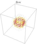
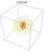
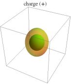
$\underline{~{}~{}~{}~{}~{}~{}~{}~{}~{}~{}~{}~{}~{}~{}~{}~{}~{}~{}~{}~{}~{}~{}~{}~{}~{}~{}~{}~{}~{}~{}~{}~{}~{}~{}~{}~{}~{}~{}~{}~{}~{}~{}~{}~{}~{}~{}~{}~{}~{}~{}~{}~{}~{}~{}~{}~{}~{}~{}~{}~{}~{}~{}~{}~{}~{}~{}~{}~{}~{}~{}~{}~{}~{}~{}~{}~{}~{}~{}~{}~{}~{}~{}~{}~{}~{}~{}~{}~{}~{}~{}~{}~{}}$

(b)      

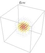
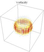
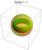
$\underline{~{}~{}~{}~{}~{}~{}~{}~{}~{}~{}~{}~{}~{}~{}~{}~{}~{}~{}~{}~{}~{}~{}~{}~{}~{}~{}~{}~{}~{}~{}~{}~{}~{}~{}~{}~{}~{}~{}~{}~{}~{}~{}~{}~{}~{}~{}~{}~{}~{}~{}~{}~{}~{}~{}~{}~{}~{}~{}~{}~{}~{}~{}~{}~{}~{}~{}~{}~{}~{}~{}~{}~{}~{}~{}~{}~{}~{}~{}~{}~{}~{}~{}~{}~{}~{}~{}~{}~{}~{}~{}~{}~{}}$

(c)      

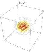
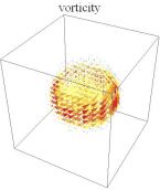
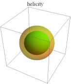
Figure 3: (a) An example of localized epi-2D flow with $\bm{V}_{1}=p\nabla q$, where $p=(x^{2}+y^{2})\phi(\sqrt{x^{2}+y^{2}+z^{2}})$ and $q=\arctan(x/y)$, which gives a primarily circulating flow. Here $\phi(\tau)=\exp[-1/(1-|\tau|^{2})]$ for $|\tau|<1$, while $\phi(\tau)=0$ for $|\tau|\geq 1$, using the Friedrichs mollifier. The contours show the levels $\mathscr{Q}_{+}=-0.1$ and $-0.5$. (b) An example of localized epi-2D flow with $\bm{V}_{2}=r\nabla s$, where $r=\phi(\sqrt{x^{2}+y^{2}+z^{2}})$ and $s=\tanh z$, which gives a primarily longitudinal flow. The contours show the levels $\mathscr{Q}_{-}=-0.1$ and $-1$. (c) An example of localized 3D flow that is generated by the fusion (superposition) of $\bm{V}_{1}$ and $\bm{V}_{2}$, generating a finite helicity density. The contours show the levels $\mathscr{C}=-0.01$ and $-0.1$.

(a)      

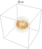
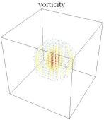
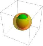
$\underline{~{}~{}~{}~{}~{}~{}~{}~{}~{}~{}~{}~{}~{}~{}~{}~{}~{}~{}~{}~{}~{}~{}~{}~{}~{}~{}~{}~{}~{}~{}~{}~{}~{}~{}~{}~{}~{}~{}~{}~{}~{}~{}~{}~{}~{}~{}~{}~{}~{}~{}~{}~{}~{}~{}~{}~{}~{}~{}~{}~{}~{}~{}~{}~{}~{}~{}~{}~{}~{}~{}~{}~{}~{}~{}~{}~{}~{}~{}~{}~{}~{}~{}~{}~{}~{}~{}~{}~{}~{}~{}~{}~{}}$

(b)      

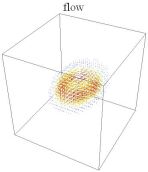
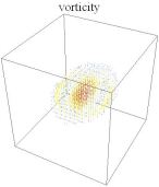
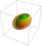
$\underline{~{}~{}~{}~{}~{}~{}~{}~{}~{}~{}~{}~{}~{}~{}~{}~{}~{}~{}~{}~{}~{}~{}~{}~{}~{}~{}~{}~{}~{}~{}~{}~{}~{}~{}~{}~{}~{}~{}~{}~{}~{}~{}~{}~{}~{}~{}~{}~{}~{}~{}~{}~{}~{}~{}~{}~{}~{}~{}~{}~{}~{}~{}~{}~{}~{}~{}~{}~{}~{}~{}~{}~{}~{}~{}~{}~{}~{}~{}~{}~{}~{}~{}~{}~{}~{}~{}~{}~{}~{}~{}~{}~{}}$

(c)      

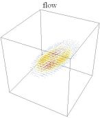
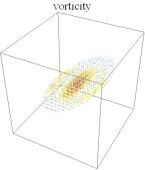
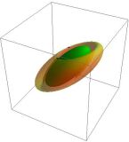
Figure 4: Deformation by a potential flow $\bm{V}_{0}=\nabla(yz)$ of an epi-2D particle $\bm{V}_{1}=p\nabla q$ with (a) the initial condition $p=(x^{2}+y^{2})\phi(\sqrt{x^{2}+y^{2}+z^{2}})$ and $q=\arctan(x/y)$. The contours $\mathscr{Q}_{+}=\pm 0.1$ are shown. (b) The deformed particle at $t=0.2$. Here we assume that $p$ and $q$ are passive scalars transported by $\bm{V}_{0}$. The deformation is written as $y\mapsto(\cosh t)y-(\sinh t)z$, and $z\mapsto-(\sinh t)y+(\cosh t)z$. (c) The deformed particle at $t=0.5$.

$~{}~{}~{}~{}~{}~{}\bm{V}~{}~{}~{}~{}~{}~{}~{}~{}~{}~{}~{}~{}~{}~{}~{}~{}~{}~{}~{}~{}~{}~{}\bm{\omega}~{}~{}~{}~{}~{}~{}~{}~{}~{}~{}~{}~{}~{}~{}~{}~{}~{}~{}~{}~{}\mathscr{Q}_{+}~{}~{}~{}~{}~{}~{}~{}~{}~{}~{}~{}~{}~{}~{}~{}~{}~{}~{}~{}\mathscr{Q}_{-}~{}~{}~{}~{}~{}~{}~{}~{}~{}~{}~{}~{}~{}~{}~{}~{}~{}~{}\mathscr{C}$

$\underline{~{}~{}~{}~{}~{}~{}~{}~{}~{}~{}~{}~{}~{}~{}~{}~{}~{}~{}~{}~{}~{}~{}~{}~{}~{}~{}~{}~{}~{}~{}~{}~{}~{}~{}~{}~{}~{}~{}~{}~{}~{}~{}~{}~{}~{}~{}~{}~{}~{}~{}~{}~{}~{}~{}~{}~{}~{}~{}~{}~{}~{}~{}~{}~{}~{}~{}~{}~{}~{}~{}~{}~{}~{}~{}~{}~{}~{}~{}~{}~{}~{}~{}~{}~{}~{}~{}~{}~{}~{}~{}~{}~{}~{}~{}~{}~{}~{}~{}~{}~{}~{}~{}~{}~{}~{}~{}~{}}$

(a)          

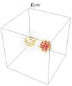
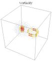
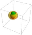
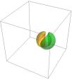
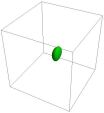
$\underline{~{}~{}~{}~{}~{}~{}~{}~{}~{}~{}~{}~{}~{}~{}~{}~{}~{}~{}~{}~{}~{}~{}~{}~{}~{}~{}~{}~{}~{}~{}~{}~{}~{}~{}~{}~{}~{}~{}~{}~{}~{}~{}~{}~{}~{}~{}~{}~{}~{}~{}~{}~{}~{}~{}~{}~{}~{}~{}~{}~{}~{}~{}~{}~{}~{}~{}~{}~{}~{}~{}~{}~{}~{}~{}~{}~{}~{}~{}~{}~{}~{}~{}~{}~{}~{}~{}~{}~{}~{}~{}~{}~{}~{}~{}~{}~{}~{}~{}~{}~{}~{}~{}~{}~{}~{}~{}~{}}$

(b)          

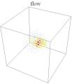
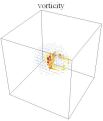
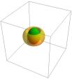
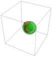
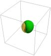
$\underline{~{}~{}~{}~{}~{}~{}~{}~{}~{}~{}~{}~{}~{}~{}~{}~{}~{}~{}~{}~{}~{}~{}~{}~{}~{}~{}~{}~{}~{}~{}~{}~{}~{}~{}~{}~{}~{}~{}~{}~{}~{}~{}~{}~{}~{}~{}~{}~{}~{}~{}~{}~{}~{}~{}~{}~{}~{}~{}~{}~{}~{}~{}~{}~{}~{}~{}~{}~{}~{}~{}~{}~{}~{}~{}~{}~{}~{}~{}~{}~{}~{}~{}~{}~{}~{}~{}~{}~{}~{}~{}~{}~{}~{}~{}~{}~{}~{}~{}~{}~{}~{}~{}~{}~{}~{}~{}~{}}$

(c)          

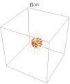
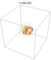
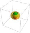
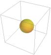
$\underline{~{}~{}~{}~{}~{}~{}~{}~{}~{}~{}~{}~{}~{}~{}~{}~{}~{}~{}~{}~{}~{}~{}~{}~{}~{}~{}~{}~{}~{}~{}~{}~{}~{}~{}~{}~{}~{}~{}~{}~{}~{}~{}~{}~{}~{}~{}~{}~{}~{}~{}~{}~{}~{}~{}~{}~{}~{}~{}~{}~{}~{}~{}~{}~{}~{}~{}~{}~{}~{}~{}~{}~{}~{}~{}~{}~{}~{}~{}~{}~{}~{}~{}~{}~{}~{}~{}~{}~{}~{}~{}~{}~{}~{}~{}~{}~{}~{}~{}~{}~{}~{}~{}~{}~{}~{}~{}~{}}$

(d)          

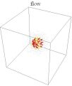
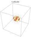
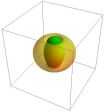
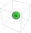
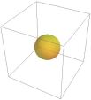
Figure 5: Fusion of circulating and longitudinal epi-2D particles with $p=\alpha(x_{1}^{2}+y^{2})\mathrm{e}^{-(x_{1}^{2}+y^{2}+z^{2})^{2}}$, $q=\arctan(x_{1}/y)$, $r=\mathrm{e}^{-(x_{2}^{2}+y^{2}+z^{2})^{4}}$, and $s=\tanh(z/2)$, where $x_{1}=x+\delta$, $x_{2}=x-\delta$. Here $\alpha=0.8$ was chosen to balance the magnitudes of both charges. The merging parameter $\delta$ is chosen in (a) $\delta=1.2$, (b) $\delta=0.5$, (c) $\delta=0.1$, (d) $\delta=0$. Contours $\mathscr{Q}_{\pm}=\pm 0.1$ and $\mathscr{C}_{\mathrm{r}}=10^{-3}$ (for $\delta=1.2$), $\pm 10^{-3}$ (for $\delta=0.5$), $-10^{-3}$ (for $\delta=0.1$ and $0$) are shown.

$~{}~{}~{}~{}~{}~{}\bm{V}~{}~{}~{}~{}~{}~{}~{}~{}~{}~{}~{}~{}~{}~{}~{}~{}~{}~{}~{}~{}~{}~{}\bm{\omega}~{}~{}~{}~{}~{}~{}~{}~{}~{}~{}~{}~{}~{}~{}~{}~{}~{}~{}~{}~{}\mathscr{Q}_{+}~{}~{}~{}~{}~{}~{}~{}~{}~{}~{}~{}~{}~{}~{}~{}~{}~{}~{}~{}\mathscr{Q}_{-}~{}~{}~{}~{}~{}~{}~{}~{}~{}~{}~{}~{}~{}~{}~{}~{}~{}~{}\mathscr{C}$

$\underline{~{}~{}~{}~{}~{}~{}~{}~{}~{}~{}~{}~{}~{}~{}~{}~{}~{}~{}~{}~{}~{}~{}~{}~{}~{}~{}~{}~{}~{}~{}~{}~{}~{}~{}~{}~{}~{}~{}~{}~{}~{}~{}~{}~{}~{}~{}~{}~{}~{}~{}~{}~{}~{}~{}~{}~{}~{}~{}~{}~{}~{}~{}~{}~{}~{}~{}~{}~{}~{}~{}~{}~{}~{}~{}~{}~{}~{}~{}~{}~{}~{}~{}~{}~{}~{}~{}~{}~{}~{}~{}~{}~{}~{}~{}~{}~{}~{}~{}~{}~{}~{}~{}~{}~{}~{}~{}~{}}$

(a)          

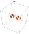
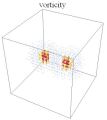
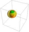
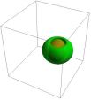
$\underline{~{}~{}~{}~{}~{}~{}~{}~{}~{}~{}~{}~{}~{}~{}~{}~{}~{}~{}~{}~{}~{}~{}~{}~{}~{}~{}~{}~{}~{}~{}~{}~{}~{}~{}~{}~{}~{}~{}~{}~{}~{}~{}~{}~{}~{}~{}~{}~{}~{}~{}~{}~{}~{}~{}~{}~{}~{}~{}~{}~{}~{}~{}~{}~{}~{}~{}~{}~{}~{}~{}~{}~{}~{}~{}~{}~{}~{}~{}~{}~{}~{}~{}~{}~{}~{}~{}~{}~{}~{}~{}~{}~{}~{}~{}~{}~{}~{}~{}~{}~{}~{}~{}~{}~{}~{}~{}~{}}$

(b)          

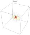
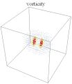
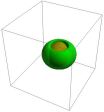
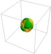
$\underline{~{}~{}~{}~{}~{}~{}~{}~{}~{}~{}~{}~{}~{}~{}~{}~{}~{}~{}~{}~{}~{}~{}~{}~{}~{}~{}~{}~{}~{}~{}~{}~{}~{}~{}~{}~{}~{}~{}~{}~{}~{}~{}~{}~{}~{}~{}~{}~{}~{}~{}~{}~{}~{}~{}~{}~{}~{}~{}~{}~{}~{}~{}~{}~{}~{}~{}~{}~{}~{}~{}~{}~{}~{}~{}~{}~{}~{}~{}~{}~{}~{}~{}~{}~{}~{}~{}~{}~{}~{}~{}~{}~{}~{}~{}~{}~{}~{}~{}~{}~{}~{}~{}~{}~{}~{}~{}~{}}$

(c)          

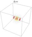
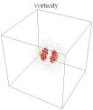
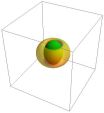
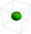
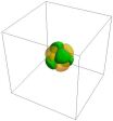
$\underline{~{}~{}~{}~{}~{}~{}~{}~{}~{}~{}~{}~{}~{}~{}~{}~{}~{}~{}~{}~{}~{}~{}~{}~{}~{}~{}~{}~{}~{}~{}~{}~{}~{}~{}~{}~{}~{}~{}~{}~{}~{}~{}~{}~{}~{}~{}~{}~{}~{}~{}~{}~{}~{}~{}~{}~{}~{}~{}~{}~{}~{}~{}~{}~{}~{}~{}~{}~{}~{}~{}~{}~{}~{}~{}~{}~{}~{}~{}~{}~{}~{}~{}~{}~{}~{}~{}~{}~{}~{}~{}~{}~{}~{}~{}~{}~{}~{}~{}~{}~{}~{}~{}~{}~{}~{}~{}~{}}$

(d)          

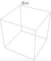
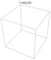
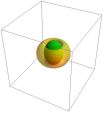
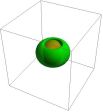
Figure 6: The fusion of a pair of epi-2D particles that circulate in the opposite directions with $p=(x_{1}^{2}+y^{2})\mathrm{e}^{-(x_{1}^{2}+y^{2}+z^{2})^{4}}$, $q=\arctan(x_{1}/y)$, $r=\alpha(x_{2}^{2}+y^{2})\mathrm{e}^{-(x_{2}^{2}+y^{2}+z^{2})^{4}}$, and $s=-\arctan(x_{2}/y)$, where $x_{1}=x+\delta$, $x_{2}=x-\delta$. The charges are evaluated as $\mathscr{Q}_{+}=\mathrm{d}p\wedge\mathrm{d}q\wedge\mathrm{d}\tau$ and $\mathscr{Q}_{-}=\mathrm{d}r\wedge\mathrm{d}s\wedge\mathrm{d}\tau$ with $\tau=\tanh z$. The merging parameter $\delta$ is chosen in (a) $\delta=1.2$, (b) $\delta=0.5$, (c) $\delta=0.1$, (d) $\delta=0$. Contours $\mathscr{Q}_{\pm}=\pm 0.1$ and $\mathscr{C}_{\mathrm{r}}=\pm 10^{-3}$ are shown.

$~{}~{}~{}~{}~{}~{}\bm{V}~{}~{}~{}~{}~{}~{}~{}~{}~{}~{}~{}~{}~{}~{}~{}~{}~{}~{}~{}~{}~{}~{}\bm{\omega}~{}~{}~{}~{}~{}~{}~{}~{}~{}~{}~{}~{}~{}~{}~{}~{}~{}~{}~{}~{}\mathscr{Q}_{+}~{}~{}~{}~{}~{}~{}~{}~{}~{}~{}~{}~{}~{}~{}~{}~{}~{}~{}~{}\mathscr{Q}_{-}~{}~{}~{}~{}~{}~{}~{}~{}~{}~{}~{}~{}~{}~{}~{}~{}~{}~{}\mathscr{C}$

$\underline{~{}~{}~{}~{}~{}~{}~{}~{}~{}~{}~{}~{}~{}~{}~{}~{}~{}~{}~{}~{}~{}~{}~{}~{}~{}~{}~{}~{}~{}~{}~{}~{}~{}~{}~{}~{}~{}~{}~{}~{}~{}~{}~{}~{}~{}~{}~{}~{}~{}~{}~{}~{}~{}~{}~{}~{}~{}~{}~{}~{}~{}~{}~{}~{}~{}~{}~{}~{}~{}~{}~{}~{}~{}~{}~{}~{}~{}~{}~{}~{}~{}~{}~{}~{}~{}~{}~{}~{}~{}~{}~{}~{}~{}~{}~{}~{}~{}~{}~{}~{}~{}~{}~{}~{}~{}~{}~{}}$

(a)          

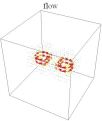
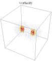
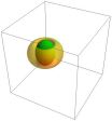
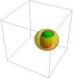
$\underline{~{}~{}~{}~{}~{}~{}~{}~{}~{}~{}~{}~{}~{}~{}~{}~{}~{}~{}~{}~{}~{}~{}~{}~{}~{}~{}~{}~{}~{}~{}~{}~{}~{}~{}~{}~{}~{}~{}~{}~{}~{}~{}~{}~{}~{}~{}~{}~{}~{}~{}~{}~{}~{}~{}~{}~{}~{}~{}~{}~{}~{}~{}~{}~{}~{}~{}~{}~{}~{}~{}~{}~{}~{}~{}~{}~{}~{}~{}~{}~{}~{}~{}~{}~{}~{}~{}~{}~{}~{}~{}~{}~{}~{}~{}~{}~{}~{}~{}~{}~{}~{}~{}~{}~{}~{}~{}~{}}$

(b)          

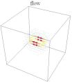
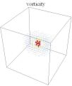
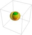
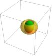
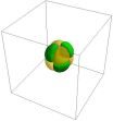
$\underline{~{}~{}~{}~{}~{}~{}~{}~{}~{}~{}~{}~{}~{}~{}~{}~{}~{}~{}~{}~{}~{}~{}~{}~{}~{}~{}~{}~{}~{}~{}~{}~{}~{}~{}~{}~{}~{}~{}~{}~{}~{}~{}~{}~{}~{}~{}~{}~{}~{}~{}~{}~{}~{}~{}~{}~{}~{}~{}~{}~{}~{}~{}~{}~{}~{}~{}~{}~{}~{}~{}~{}~{}~{}~{}~{}~{}~{}~{}~{}~{}~{}~{}~{}~{}~{}~{}~{}~{}~{}~{}~{}~{}~{}~{}~{}~{}~{}~{}~{}~{}~{}~{}~{}~{}~{}~{}~{}}$

(c)          

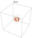
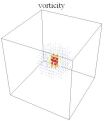
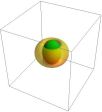
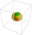
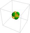
$\underline{~{}~{}~{}~{}~{}~{}~{}~{}~{}~{}~{}~{}~{}~{}~{}~{}~{}~{}~{}~{}~{}~{}~{}~{}~{}~{}~{}~{}~{}~{}~{}~{}~{}~{}~{}~{}~{}~{}~{}~{}~{}~{}~{}~{}~{}~{}~{}~{}~{}~{}~{}~{}~{}~{}~{}~{}~{}~{}~{}~{}~{}~{}~{}~{}~{}~{}~{}~{}~{}~{}~{}~{}~{}~{}~{}~{}~{}~{}~{}~{}~{}~{}~{}~{}~{}~{}~{}~{}~{}~{}~{}~{}~{}~{}~{}~{}~{}~{}~{}~{}~{}~{}~{}~{}~{}~{}~{}}$

(d)          

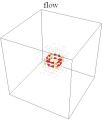
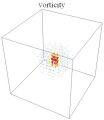
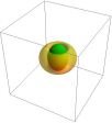
Figure 7: Fusion of a pair of epi-2D particles that circulate in the same directions with $p=(x_{1}^{2}+y^{2})\mathrm{e}^{-(x_{1}^{2}+y^{2}+z^{2})^{4}}$, $q=\arctan(x_{1}/y)$, $r=\alpha(x_{2}^{2}+y^{2})\mathrm{e}^{-(x_{2}^{2}+y^{2}+z^{2})^{4}}$, and $s=\arctan(x_{2}/y)$, where $x_{1}=x+\delta$, $x_{2}=x-\delta$. The charges are evaluated as $\mathscr{Q}_{+}=\mathrm{d}p\wedge\mathrm{d}q\wedge\mathrm{d}\tau$ and $\mathscr{Q}_{-}=\mathrm{d}r\wedge\mathrm{d}s\wedge\mathrm{d}\tau$ with $\tau=\tanh z$. The merging parameter $\delta$ is chosen in (a) $\delta=1.2$, (b) $\delta=0.5$, (c) $\delta=0.1$, (d) $\delta=0$. Contours of $\mathscr{Q}_{\pm}=\pm 0.1$ and $\mathscr{C}_{\mathrm{r}}=\pm 10^{-3}$ are shown. As $p=\alpha r$ ($\alpha=$ constant) at $\delta=0$, the fusion of $\mathscr{Q}_{+}$ and $\mathscr{Q}_{-}$ yields zero helicity.

References

(1)
A. Hasegawa,
Adv. Phys. 34, 1(1985).
(2)
The alignment of vorticity vectors is one of the characteristics of 2D-like flow,
causing the suppression of blowup singularity (P. Constantin and C. Fefferman,
Indiana Univ. Math. J. 42, 775 (1993)).
(3)
J.J. Moreau,
C. R. Acad. Sci. Paris 252, 2810 (1961).
(4)
The first use of the helicity in classical field theory was for
characterizing stellar magnetic fields (L. Woltjer, Proc. Natl. Acad. Sci. U.S.A. 44, 489 (1958)).
(5)
The helicity and the enstrophy can be unified as cross helicities (Y. Fukumoto,
Topologica 1 003 (2008)).
But here we focus on their difference and metamorphose.
(6)
See Appendix A for the problems pertinent to boundary conditions.
(7)
P.J. Morrison and J.M. Greene,
Phys. Rev. Lett. 45, 790 (1980).
(9)
N. Padhye and P. J. Morrison,
Phys. Lett. A,
219, 287 (1996);
Plasma Phys. Reports,
22, 869 (1996).
(10)
A. Clebsch,
Z. Reine Angew. Math. 54, 293 (1857).
(11)
P. J. Morrison,
AIP Conf. Proc. 88, 13
(1982).
(12)
J. Marsden and A Weinstein,
Physica D 7, 305 (1983).
(13)
Z. Yoshida,
J. Math. Phys. 50, 113101 (2009).
(14)
The Clebsch parameters mediate the correspondence between classical fields and quantum fields; cf.
R. Jackiw, V.P. Nair, S.-Y. Pi, and A.P. Polychronakos,
J. Phys. A: Math. Gen. 37, R327 (2004);
Z. Yoshida and S. M. Mahajan,
J. Phys. A: Math. Theor. 49, 055501 (2016).
(15)
The variation of the action due to the Hamiltonian vector generated by (or ) yields an
exact current density (3-form in the 4D space-time), whose spatial integral is the Noether current.
The 0th (temporal) component of the Noether current is the Noether charge which turns out to be (or ) itself;
K. Tanehashi and Z. Yoshida,
J. Phys. A: Math. Theor. 48, 495501 (2015).
(16)
A deeper mathematical structure is elucidated by formulating the system in terms of differential forms;
see Appendix B.
(17)
C.C. Lin,
in Proc. Int. Sch. Phys. “Enrico Fermi” XXI,
(Academic Press, New York, 1963) pp. 93.
(19)
By epi-2D we mean a class ‘over’ 2D.
It is different from the so-called ‘2.5D’ class of fields that are defined on a 2D base space but have 3 components,
or the class of fields that have some continuous symmetry by which the number of independent variables can be reduced to two;
see, for example,
B. Ettinger and E.S. Titi,
SIAM J. Math. Anal. 41, 269 (2009).
(20)
Z. Yoshida and P.J. Morrison,
Fluid Dyn. Res. 46, 031412 (2014).
(21)
T. Dombre, U. Frisch, J. M. Greene, M. Hénon, A. Mehr, and A. M. Soward,
J. Fluid Mech. 167, 353 (1986).
(22)
Historically, Kelvin called a vorticity-free flow (, or ) a lamellar field,
and a helicity-free flow (, or ) a complex lamellar field.
The epi-2D flow is the combination of a lamellar field and a complex lamellar field.
The Clebsch parameters and may be called Monge’s potentials;
see
C. Truesdell,
The kinematics of vorticity,
(Indiana Univ. Press, Bloomington, 1954), Chap. I.
(23)
An axisymmetric flow such that and is also 2D, in which
we may choose , and then, the enstrophy of
is constant.
A helically symmetric flow
such that and
( with a constant )
is epi-2D,
which can be written as
with and being functions of and .
It is not 2D, because is not integrable to define a perpendicular 2D manifold,
however, it is very close to 2D in that the vortex stretching vanishes;
cf. 2.5D .
(24)
By Frobenius’ theorem,
the following two conditions are equivalent for a 1-form on a 3D manifold:
(1) is helicity free ().
(2) is locally integrable, i.e.,
().
An epi-2D flow consists of a helicity-free flow and a potential flow,
which may be viewed as a Pfaffian form (C. Carathéodory, Calculus of Variations and Partial Differential Equations of the First Order, 3rd Ed.
(AMS Chelsea Publishing, Providence, 2002)).
See also Appendix B.
(25)
See Appendix C for graphical images of epi-2D particles and their fusion.
(26)
D. Kleckner and W.T.M. Irvine,
Nat. Phys. 9, 253 (2013).
(27)
S. Douady, Y. Couder, and M.E. Brachet,
Phys. Rev. Lett. 67, 983 (1991).
(28)
Y. Hattori and H.K. Moffatt,
Fluid Dyn. Res. 26, 333 (2005).
(29)
Y. Kimura and H.K. Moffatt,
J. Fluid Mech. 751, 329 (2014).
(30)
M. Farge, G. Pellegrino, and K. Schneider,
Phys. Rev. Lett. 87, 054501 (2001).
(31)
H.K. Moffatt, J. Plasma Phys. 81, 905810608 (2015).
(32)
K. Toyoda, F. Takahashi, S. Takizawa, Y. Tokizane, K. Miyamoto, R. Morita, T. Omatsu,
Phys. Rev. Lett. 110, 143603 (2013).
(33)
J. Ishioka, Y. H. Liu, K. Shimatake, T. Kurosawa, K. Ichimura, Y. Toda, M. Oda, and S. Tanda,
Phys. Rev. Lett. 105, 176401 (2010).