Exploratory studies for the position-space approach to hadronic light-by-light scattering in the muon $g-2$

Abstract

The well-known discrepancy in the muon $g-2$ between experiment and theory demands further theory investigations in view of the upcoming new experiments. One of the leading uncertainties lies in the hadronic light-by-light scattering contribution (HLbL), that we address with our position-space approach. We focus on exploratory studies of the pion-pole contribution in a simple model and the fermion loop without gluon exchanges in the continuum and in infinite volume. These studies provide us with useful information for our planned computation of HLbL in the muon $g-2$ using full QCD.

1 Introduction

The anomalous magnetic moment of the muon $a_{\mu}=\frac{g_{\mu}-2}{2}$ provides a high-precision test of the Standard Model. Current experiments and Standard-Model computations show a discrepancy of about three standard deviations; see Ref. Jegerlehner:2017lbd and references therein. This leads to the question whether this is a hint of new physics or just a statistical or systematic fluctuation from the exact value. To address this question, the uncertainty on this value has to be reduced. Experiments at Fermilab and at J-PARC plan to improve on the uncertainty by a factor of fourhertzog:2015jru . The theoretical prediction ought to be improved in equal measure. The theoretical uncertainty is dominated by the hadronic vacuum polarization contribution (HVP) and the hadronic light-by-light contribution (HLbL).

Lattice QCD can provide a first-principle estimate of $a_{\mu}^{\text{HLbL}}$ Blum:2014oka ; Blum:2015gfa ; Blum:2016lnc ; Blum:2017cer ; Asmussen:2015 ; Green:2015mva ; Asmussen:2016lse . Other methods rely on models, because the HLbL is not fully related to any cross section, leading to large uncertainties. Dispersion relations allow one to use experimental data to reduce the uncertainties for the dominant contributions ($\pi^{0}\,,\,\eta\,,\,\eta^{\prime}\,;\,\pi\pi$), see Colangelo et al. Colangelo:2014dfa ; Colangelo:2014pva ; Colangelo:2015ama ; Colangelo:2017qdm ; Colangelo:2017fiz and Pauk and Vanderhaeghen Pauk:2014rfa . Results from lattice QCD can be used as inputs to Gerardin:2016cqj or tests of Green:2015sra these dispersive approaches. More challenging is a full calculation of $a_{\mu}^{\text{HLbL}}$; in these proceedings, we report our progress towards such a calculation.

2 Expression for $a_{\mu}^{\text{HLbL}}$ in Euclidean position space

The HLbL can be split into a continuum, infinite volume QED kernel function $\bar{\cal L}$ and a (Lattice) QCD four-point correlation function $i\widehat{\Pi}$; see Fig. 1. The anomalous magnetic moment $a_{\mu}^{\text{HLbL}}$ can then be computed from our master formula:

$$a_{\mu}^{\text{HLbL}}= F_{2}(0)=\frac{me^{6}}{3}\underbrace{\int d^{4}y}_{=2\pi^{2}\int_{0}^{\infty}d|y||y|^{3}}\Big{[}\underbrace{\int d^{4}x}_{\mathclap{\raisebox{-3.5pt}{\scriptsize$\hskip 56.00012pt=4\pi\int_{0}^{\pi}d\beta\sin^{2}(\beta)\int_{0}^{\infty}d\lvert x\rvert\lvert x\rvert^{3}$}}}\underbrace{\bar{\cal L}_{[\rho,\sigma];\mu\nu\lambda}(x,y)}_{\rm QED}\;\underbrace{i\widehat{\Pi}_{\rho;\mu\nu\lambda\sigma}(x,y)}_{\rm QCD}\Big{]},$$ (1)

$$i\widehat{\Pi}_{\rho;\mu\nu\lambda\sigma}(x,y)= -\int d^{4}z\;z_{\rho}\,\Big{\langle}\,j_{\mu}(x)\,j_{\nu}(y)\,j_{\sigma}(z)\,j_{\lambda}(0)\Big{\rangle}.$$ (2)

For information on the derivation of the master formula, see our Lattice 2016 proceedings contribution Asmussen:2016lse . Note, that by treating the QED kernel function in infinite volume, we avoid introducing $\frac{1}{L^{2}}$ finite-volume effects due to the photons. In the derivation we made the Lorentz covariance manifest, which allows us to reduce the eight-dimensional integral to an integral in three dimensions, as annotated in formula (1). In a Lattice QCD computation of the fully connected diagrams, one would evaluate the four-dimensional $x$ integral with the help of sequential propagators and only reduce the $y$ integral to one dimension. The square brackets in formula (1) can be evaluated in one step for one value of $y$. This makes it affordable to sample the integrand for the remaining one-dimensional integral over $y$.

\begin{overpic}[width=156.10345pt]{muonhlbl.pdf} \put(39.0,24.0){\small$x$} \put(53.0,20.0){\small$y$} \put(59.0,26.0){\small$0$} \put(51.0,42.0){\small$z$} \end{overpic}

Figure 1: Hadronic light-by-light scattering in the $(g-2)_{\mu}$. The muon and the photon propagators are contained in the QED kernel function $\bar{\mathcal{L}}$. The blob denotes the QCD correlation function $i\hat{\Pi}$ to be evaluated on the lattice.

The kernel function $\bar{\mathcal{L}}$ is decomposed into tensors:

$$\bar{\cal L}_{[\rho,\sigma];\mu\nu\lambda}(x,y)=\sum_{A={\rm I,II,III}}{\cal G}^{A}_{\delta[\rho\sigma]\mu\alpha\nu\beta\lambda}T^{(A)}_{\alpha\beta\delta}(x,y),$$ (3)

with e. g.

$${\cal G}^{\rm I}_{\delta[\rho\sigma]\mu\alpha\nu\beta\lambda} \equiv {\frac{1}{8}}{\rm Tr}\Big{\{}\Big{(}\gamma_{\delta}[\gamma_{\rho},\gamma_{\sigma}]+2(\delta_{\delta\sigma}\gamma_{\rho}-\delta_{\delta\rho}\gamma_{\sigma})\Big{)}\gamma_{\mu}\gamma_{\alpha}\gamma_{\nu}\gamma_{\beta}\gamma_{\lambda}\Big{\}}.$$ (4)

The trace of the gamma matrices evaluates to sums of products of Kronecker deltas.

The tensors $T^{(A)}$ in turn are decomposed into a scalar $S$, vector $V$ and tensor $T$ contribution,

$$T^{({\rm I})}_{\alpha\beta\delta}(x,y) = \partial^{(x)}_{\alpha}(\partial^{(x)}_{\beta}+\partial^{(y)}_{\beta})V_{\delta}(x,y),$$ (5)

$$T^{({\rm II})}_{\alpha\beta\delta}(x,y) = m\partial^{(x)}_{\alpha}\Big{(}T_{\beta\delta}(x,y)+\frac{1}{4}\delta_{\beta\delta}S(x,y)\Big{)},$$ (6)

$$T^{({\rm III})}_{\alpha\beta\delta}(x,y) = m(\partial^{(x)}_{\beta}+\partial^{(y)}_{\beta})\Big{(}T_{\alpha\delta}(x,y)+\frac{1}{4}\delta_{\alpha\delta}S(x,y)\Big{)}.$$ (7)

The latter are parametrized by the six weight functions $\bar{\mathfrak{g}}^{(0,1,2)}$, $\bar{\mathfrak{l}}^{(1,2,3)}$:

$$S(x,y) =\bar{\mathfrak{g}}^{(0)}(|x|,\hat{x}\cdot\hat{y},|y|),\phantom{\frac{1}{1}}$$ (8)

$$V_{\delta}(x,y) =x_{\delta}\bar{\mathfrak{g}}^{(1)}(|x|,\hat{x}\cdot\hat{y},|y|)+y_{\delta}\bar{\mathfrak{g}}^{(2)}(|x|,\hat{x}\cdot\hat{y},|y|),$$ (9)

$$T_{\alpha\beta}(x,y) =(x_{\alpha}x_{\beta}-\frac{x^{2}}{4}\delta_{\alpha\beta})\;\bar{\mathfrak{l}}^{(1)}+(y_{\alpha}y_{\beta}-\frac{y^{2}}{4}\delta_{\alpha\beta})\;\bar{\mathfrak{l}}^{(2)}+(x_{\alpha}y_{\beta}+y_{\alpha}x_{\beta}-\frac{x\cdot y}{2}\delta_{\alpha\beta})\;\bar{\mathfrak{l}}^{(3)},$$ (10)

where $\hat{x}=\frac{x}{\lvert x\rvert}$ and $\hat{y}=\frac{y}{\lvert y\rvert}$. To evaluate the QED kernel $\bar{\cal L}_{[\rho,\sigma];\mu\nu\lambda}(x,y)$ we compute and store all six weight functions; the remaining operations to get the QED kernel are computationally inexpensive and it is convenient to perform them during the lattice computation. Due to the Lorentz covariance, the six weight functions $\bar{\mathfrak{g}}^{(0,1,2)}$ and $\bar{\mathfrak{l}}^{(1,2,3)}$ are functions of the three parameters $x^{2}$, $y^{2}$ and $x\cdot y$ only. Therefore, it is feasible to precompute and store them. Plots of all six weight functions are shown in Fig. 2.

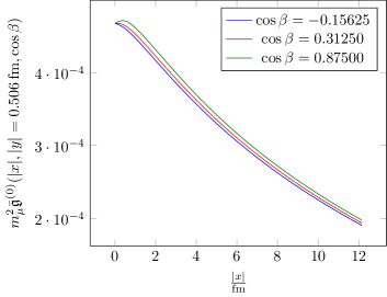
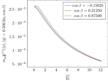
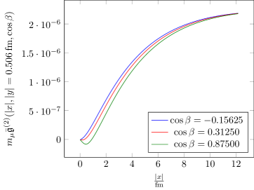
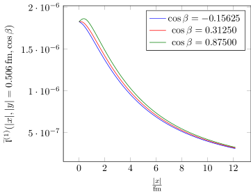
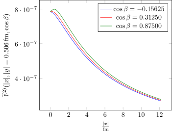
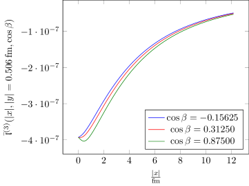
Figure 2: The $\lvert x\rvert$ dependence of all six weight functions for $\lvert y\rvert=$0.506\text{\,}\mathrm{f}\mathrm{m}$$ and three values of $\cos\beta$. Note that $\bar{\mathfrak{g}}^{(0)}$ contains an arbitrary additive constant, because of a regulated infrared divergence present before taking the derivatives in Eqs. (5–7).

3 Numerical tests

To verify that the method and its implementation are correct, we computed the $\pi^{0}$-pole contribution in the vector-meson-dominance model as well as the lepton-loop contribution to $a_{\mu}^{\text{LbL}}$ in QED. These results can be compared with the known values of these contributions.

3.1 The $\pi^{0}$-pole contribution

The first check is the $\pi^{0}$-pole contribution assuming a vector-meson-dominance transition form factor (parameters: $m_{V}$, $m_{\pi}$ and overall normalization),

$${\cal F}(-q_{1}^{2},-q_{2}^{2})=\frac{c_{\pi}}{(q_{1}^{2}+m_{V}^{2})(q_{2}^{2}+m_{V}^{2})},\qquad c_{\pi}=-\frac{N_{c}m_{V}^{4}}{12\pi^{2}F_{\pi}}.$$ (11)

We construct the correlation function for the $\pi^{0}$-pole contribution. The result reads

$$i\widehat{\Pi}_{\rho;\mu\nu\lambda\sigma}(x,y)=\frac{c_{\pi}^{2}}{m_{V}^{2}(m_{V}^{2}-m_{\pi}^{2})}\frac{\partial}{\partial x_{\alpha}}\frac{\partial}{\partial y_{\beta}}\Big{\{}\epsilon_{\mu\nu\alpha\beta}\epsilon_{\sigma\lambda\rho\gamma}\Big{(}\frac{\partial}{\partial x_{\gamma}}+\frac{\partial}{\partial y_{\gamma}}\Big{)}K_{\pi}(x,y)$$

$$+\epsilon_{\mu\lambda\alpha\beta}\epsilon_{\nu\sigma\gamma\rho}\frac{\partial}{\partial y_{\gamma}}K_{\pi}(y-x,y)+\epsilon_{\mu\sigma\alpha\rho}\epsilon_{\nu\lambda\beta\gamma}\frac{\partial}{\partial x_{\gamma}}K_{\pi}(x,x-y)\Big{\}},$$ (12)

where, with the massive propagator in position space $G_{m}(x)$,

$$K_{\pi}(x,y)\equiv\int d^{4}u\Big{(}G_{m_{\pi}}(u)-G_{m_{V}}(u)\Big{)}G_{m_{V}}(x-u)G_{m_{V}}(y-u)=K_{\pi}(y,x).$$ (13)

With the correlation function at hand, we can apply the techniques described in Sec. 2. The result is shown in Fig. 3. In view of the exponential decay $\sim e^{-\tilde{c}m_{\pi}|y|}$ of the correlation function, the observed contribution to $a_{\mu}^{\text{HLbL}}$ is remarkably long-range. This demands for large lattices at the order of $5-10\,$$\mathrm{f}\mathrm{m}$ for the physical pion mass.

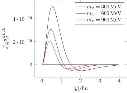
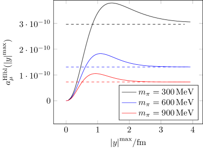
Figure 3: The $\pi^{0}$-pole contribution assuming a transition form factor given by the vector-meson-dominance model. For a cutoff choosen to be $4\text{\,}\mathrm{f}\mathrm{m}$ in the $\lvert x\rvert$ direction, the left plot shows the integrand of the $\lvert y\rvert$ integration of $a_{\mu}^{\text{HLbL}}$ and the right plot shows the value of $a_{\mu}^{\text{HLbL}}$ for an upper integration limit $\lvert y\rvert^{\text{max}}$. The dashed line represents the result from the momentum-space integration.

3.2 The lepton loop contribution in QED

The analytic result for the correlation function for a lepton loop with mass $m_{l}$ is:

$$i\widehat{\Pi}_{\rho;\mu\nu\lambda\sigma}(x,y) = \widehat{\Pi}^{(1)}_{\rho;\mu\nu\lambda\sigma}(x,y)$$ (14)

$$+\widehat{\Pi}^{(1)}_{\rho;\nu\lambda\mu\sigma}(y-x,-x)+x_{\rho}\,\Pi^{(r,1)}_{\nu\lambda\mu\sigma}(y-x,-x)$$

$$+\widehat{\Pi}^{(1)}_{\rho;\lambda\nu\mu\sigma}(-x,y-x)+x_{\rho}\,\Pi^{(r,1)}_{\lambda\nu\mu\sigma}(-x,y-x).$$

It consists of the two functions $\Pi^{(1)}$ and $\Pi^{(r,1)}$. These functions are sums of products of Bessel functions and traces of gamma matrices. The gamma matrices evaluate to sums of products of Kronecker deltas. The integral in $z$ has already been performed analytically and the evaluation boils down to computing the Bessel functions and evaluating the traces. The two functions read

$$\Pi^{(r,1)}_{\mu\nu\lambda\sigma}(x,y)=2\Big{(}\frac{m_{l}}{2\pi}\Big{)}^{8}\Big{[}$$

$$\frac{(-x_{\alpha})(x-y)_{\beta}\;K_{2}(m_{l}|x|)K_{2}(m_{l}|x-y|)}{|x|^{2}|x-y|^{2}}\cdot l_{\gamma\delta}(y)\cdot{\rm Tr}\{\gamma_{\alpha}\gamma_{\mu}\gamma_{\beta}\gamma_{\nu}\gamma_{\gamma}\gamma_{\sigma}\gamma_{\delta}\gamma_{\lambda}\}$$

$$+\frac{K_{1}(m_{l}|x|)K_{1}(m_{l}|x-y|)}{|x||x-y|}\cdot p(|y|)\cdot{\rm Tr}\{\gamma_{\mu}\gamma_{\nu}\gamma_{\sigma}\gamma_{\lambda}\}$$

$$+\frac{(-x_{\alpha})(x-y)_{\beta}\;K_{2}(m_{l}|x|)K_{2}(m_{l}|x-y|)}{|x|^{2}|x-y|^{2}}\cdot p(|y|)\cdot{\rm Tr}\{\gamma_{\alpha}\gamma_{\mu}\gamma_{\beta}\gamma_{\nu}\gamma_{\sigma}\gamma_{\lambda}\}$$

$$+\frac{(-x_{\alpha})\;K_{2}(m_{l}|x|)K_{1}(m_{l}|x-y|)}{|x|^{2}|x-y|}\cdot q_{\gamma}(y)\cdot{\rm Tr}\{\gamma_{\alpha}\gamma_{\mu}\gamma_{\nu}\gamma_{\gamma}\gamma_{\sigma}\gamma_{\lambda}\}$$

$$+\frac{(x-y)_{\beta}\;K_{1}(m_{l}|x|)K_{2}(m_{l}|x-y|)}{|x||x-y|^{2}}\cdot q_{\gamma}(y)\cdot{\rm Tr}\{\gamma_{\mu}\gamma_{\beta}\gamma_{\nu}\gamma_{\gamma}\gamma_{\sigma}\gamma_{\lambda}\}$$

$$+\frac{(-x_{\alpha})\;K_{2}(m_{l}|x|)K_{1}(m_{l}|x-y|)}{|x|^{2}|x-y|}\cdot q_{\delta}(y)\cdot{\rm Tr}\{\gamma_{\alpha}\gamma_{\mu}\gamma_{\nu}\gamma_{\sigma}\gamma_{\delta}\gamma_{\lambda}\}$$

$$+\frac{(x-y)_{\beta}\;K_{1}(m_{l}|x|)K_{2}(m_{l}|x-y|)}{|x||x-y|^{2}}\cdot q_{\delta}(y)\cdot{\rm Tr}\{\gamma_{\mu}\gamma_{\beta}\gamma_{\nu}\gamma_{\sigma}\gamma_{\delta}\gamma_{\lambda}\}$$

$$+\frac{K_{1}(m_{l}|x|)K_{1}(m_{l}|x-y|)}{|x||x-y|}\cdot l_{\gamma\delta}(y)\cdot{\rm Tr}\{\gamma_{\mu}\gamma_{\nu}\gamma_{\gamma}\gamma_{\sigma}\gamma_{\delta}\gamma_{\lambda}\}\Big{]}\,,$$ (15)

and

$$\widehat{\Pi}^{(1)}_{\rho;\mu\nu\lambda\sigma}(x,y)=2\Big{(}\frac{m_{l}}{2\pi}\Big{)}^{8}\Big{[}$$

$$\frac{(-x_{\alpha})(x-y)_{\beta}K_{2}(m_{l}|x|)K_{2}(m_{l}|x-y|)}{|x|^{2}|x-y|^{2}}\cdot{f}_{\rho\delta\gamma}(y)\cdot{\rm Tr}\{\gamma_{\alpha}\gamma_{\mu}\gamma_{\beta}\gamma_{\nu}\gamma_{\gamma}\gamma_{\sigma}\gamma_{\delta}\gamma_{\lambda}\}$$

$$+\frac{K_{1}(m_{l}|x|)K_{1}(m_{l}|x-y|)}{|x||x-y|}\cdot{f}_{\rho\delta\gamma}(y)\cdot{\rm Tr}\{\gamma_{\mu}\gamma_{\nu}\gamma_{\gamma}\gamma_{\sigma}\gamma_{\delta}\gamma_{\lambda}\}$$

$$+\frac{K_{1}(m_{l}|x|)K_{1}(m_{l}|x-y|)}{|x||x-y|}\cdot\,g_{\rho}(y)\cdot{\rm Tr}\{\gamma_{\mu}\gamma_{\nu}\gamma_{\sigma}\gamma_{\lambda}\}$$

$$+\frac{(-x_{\alpha})(x-y)_{\beta}\;K_{2}(m_{l}|x|)K_{2}(m_{l}|x-y|)}{|x|^{2}|x-y|^{2}}\cdot g_{\rho}(y)\cdot{\rm Tr}\{\gamma_{\alpha}\gamma_{\mu}\gamma_{\beta}\gamma_{\nu}\gamma_{\sigma}\gamma_{\lambda}\}$$

$$+\frac{(-x_{\alpha})\;K_{2}(m_{l}|x|)K_{1}(m_{l}|x-y|)}{|x|^{2}|x-y|}\cdot h_{\rho\gamma}(y)\cdot{\rm Tr}\{\gamma_{\alpha}\gamma_{\mu}\gamma_{\nu}\gamma_{\gamma}\gamma_{\sigma}\gamma_{\lambda}\}$$

$$+\frac{(x-y)_{\beta}\;K_{1}(m_{l}|x|)K_{2}(m_{l}|x-y|)}{|x||x-y|^{2}}\cdot h_{\rho\gamma}(y)\cdot{\rm Tr}\{\gamma_{\mu}\gamma_{\beta}\gamma_{\nu}\gamma_{\gamma}\gamma_{\sigma}\gamma_{\lambda}\}$$

$$+\frac{(-x_{\alpha})\;K_{2}(m_{l}|x|)K_{1}(m_{l}|x-y|)}{|x|^{2}|x-y|}\cdot\hat{f}_{\rho\delta}(y)\cdot{\rm Tr}\{\gamma_{\alpha}\gamma_{\mu}\gamma_{\nu}\gamma_{\sigma}\gamma_{\delta}\gamma_{\lambda}\}$$

$$+\frac{(x-y)_{\beta}\;K_{1}(m_{l}|x|)K_{2}(m_{l}|x-y|)}{|x||x-y|^{2}}\cdot\hat{f}_{\rho\delta}(y)\cdot{\rm Tr}\{\gamma_{\mu}\gamma_{\beta}\gamma_{\nu}\gamma_{\sigma}\gamma_{\delta}\gamma_{\lambda}\}\Big{]}\,,$$ (16)

where

$$l_{\gamma\delta}(y) =\frac{2\pi^{2}}{m_{l}^{2}}\Big{(}\hat{y}_{\gamma}\hat{y}_{\delta}\,K_{2}(m_{l}|y|)-\delta_{\gamma\delta}\,\frac{K_{1}(m_{l}|y|)}{m_{l}|y|}\Big{)},$$ (17)

$$h_{\rho\gamma}(y) =\frac{\pi^{2}}{m_{l}^{3}}\Big{(}\hat{y}_{\gamma}\hat{y}_{\rho}\,m_{l}|y|\,K_{1}(m_{l}|y|)-\delta_{\gamma\rho}K_{0}(m_{l}|y|)\Big{)},$$ (18)

$$\hat{f}_{\rho\delta}(y) =\frac{\pi^{2}}{m_{l}^{3}}\Big{\{}\hat{y}_{\rho}\hat{y}_{\delta}\;m_{l}|y|K_{1}(m_{l}|y|)+\delta_{\rho\delta}K_{0}(m_{l}|y|)\Big{\}},$$ (19)

$$g_{\rho}(y) =\frac{\pi^{2}}{m_{l}^{2}}\,y_{\rho}\,K_{0}(m_{l}|y|),$$ (20)

$$q_{\gamma}(y) =\frac{2\pi^{2}}{m_{l}^{2}}\,\hat{y}_{\gamma}\,K_{1}(m_{l}|y|),$$ (21)

$${f}_{\rho\delta\gamma}(y) =\frac{\pi^{2}}{m_{l}^{3}}\Big{\{}\hat{y}_{\gamma}\hat{y}_{\delta}\hat{y}_{\rho}\,m_{l}|y|K_{2}(m_{l}|y|)+(\delta_{\rho\delta}\hat{y}_{\gamma}-\delta_{\gamma\rho}\hat{y}_{\delta}-\delta_{\gamma\delta}\hat{y}_{\rho})\,K_{1}(m_{l}|y|)\Big{\}},$$ (22)

$$p(|y|) =\frac{2\pi^{2}}{m_{l}^{2}}\,K_{0}(m_{l}|y|).$$ (23)

The integrand $f(\lvert y\rvert)$ of the final $\lvert y\rvert$ integration is shown in Fig. 4. The behaviour for small $\lvert y\rvert$ is numerically compatible with $f(\lvert y\rvert)\propto m_{\mu}\lvert y\rvert\log^{2}(m_{\mu}\lvert y\rvert)$. This is quite steep and means that we probe the kernel precisely also for small distances. With this correlation function, the resulting value for $a_{\mu}^{\text{LbL}}$ for different loop masses can be reproduced at the percent level; see Table 1.

$m_{l}/m_{\mu}$	$a_{\mu}^{\text{LbL}}\times 10^{11}$ (exact)	$a_{\mu}^{\text{LbL}}\times 10^{11}$		Precision	Deviation
1	$464.97$	470.6	(2.3)(2.1)	$0.7$%	$1.2$%
2	$150.31$	150.4	(0.7)(1.7)	$1.2$%	$0.06$%

Table 1: Results for the lepton-loop contribution in QED. For the exact numbers cf. Laporta:1992pa ; Passera:PC . The first uncertainty stems from the three-dimensional integration, the second from the extrapolation to small $\lvert y\rvert$.

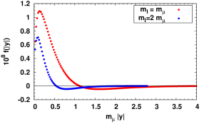
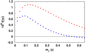
Figure 4: Integrand of the lepton loop contribution $a_{\mu}^{\text{LbL}}$ in QED. The full integration region is shown on the left, a detailed view of the small $|y|$ region on the right.

4 Conclusions

The covariant position-space method remains a promising approach to calculate the HLbL contribution to $(g-2)_{\mu}$. We did two tests of our QED kernel with the help of semi-analytic computations of the correlation function $i\hat{\Pi}$. The first test is the $\pi^{0}$-pole contribution in a vector-meson dominance model for the transition form factor, and the second is a lepton loop. We reproduce the known analytic result for the lepton loop at the percent level. One important observation is that the $\pi^{0}$-pole contribution is very long-range, but we hope to be able to correct for the finite-size effects on this contribution, by computing the transition form factor Gerardin:2016cqj on the same ensemble and using Eqs. (12, 13). We plan to make the QED kernel publicly available.

References

- (1) F. Jegerlehner, 1705.00263
- (2) D.W. Hertzog, EPJ Web Conf. 118, 01015 (2016), 1512.00928
- (3) T. Blum, S. Chowdhury, M. Hayakawa, T. Izubuchi, Phys. Rev. Lett. 114, 012001 (2015), 1407.2923
- (4) T. Blum, N. Christ, M. Hayakawa, T. Izubuchi, L. Jin, C. Lehner, Phys. Rev. D93, 014503 (2016), 1510.07100
- (5) T. Blum, N. Christ, M. Hayakawa, T. Izubuchi, L. Jin, C. Jung, C. Lehner, Phys. Rev. Lett. 118, 022005 (2017), 1610.04603
- (6) T. Blum, N. Christ, M. Hayakawa, T. Izubuchi, L. Jin, C. Jung, C. Lehner, Phys. Rev. D96, 034515 (2017), 1705.01067
- (7) N. Asmussen, J. Green, V. Gülpers, G. von Hippel, H.B. Meyer, A. Nyffeler, H. Wittig, Hadronic light-by-light contribution to the muon anomalous magnetic moment on the lattice (2015), http://www.dpg-verhandlungen.de/year/2015/conference/heidelberg/part/sydm/session/3/contribution/6
- (8) J. Green, N. Asmussen, O. Gryniuk, G. von Hippel, H.B. Meyer, A. Nyffeler, V. Pascalutsa, PoS LATTICE2015, 109 (2016), 1510.08384
- (9) N. Asmussen, J. Green, H.B. Meyer, A. Nyffeler, PoS LATTICE2016, 164 (2016), 1609.08454
- (10) G. Colangelo, M. Hoferichter, M. Procura, P. Stoffer, JHEP 09, 091 (2014), 1402.7081
- (11) G. Colangelo, M. Hoferichter, B. Kubis, M. Procura, P. Stoffer, Phys. Lett. B738, 6 (2014), 1408.2517
- (12) G. Colangelo, M. Hoferichter, M. Procura, P. Stoffer, JHEP 09, 074 (2015), 1506.01386
- (13) G. Colangelo, M. Hoferichter, M. Procura, P. Stoffer, Phys. Rev. Lett. 118, 232001 (2017), 1701.06554
- (14) G. Colangelo, M. Hoferichter, M. Procura, P. Stoffer, JHEP 04, 161 (2017), 1702.07347
- (15) V. Pauk, M. Vanderhaeghen, Phys. Rev. D90, 113012 (2014), 1409.0819
- (16) A. Gérardin, H.B. Meyer, A. Nyffeler, Phys. Rev. D94, 074507 (2016), 1607.08174
- (17) J. Green, O. Gryniuk, G. von Hippel, H.B. Meyer, V. Pascalutsa, Phys. Rev. Lett. 115, 222003 (2015), 1507.01577
- (18) S. Laporta, E. Remiddi, Phys. Lett. B301, 440 (1993)
- (19) M. Passera, private communication