Coherence generating power of unitary transformations
via probabilistic average

Abstract

We study the ability of a quantum channel to generate quantum coherence when it applies to incoherent states. Based on probabilistic averages, we define a measure of such coherence generating power (CGP) for a generic quantum channel, based on the average coherence generated by the quantum channel acting on a uniform ensemble of incoherent states. Explicit analytical formula of the CGP for any unitary channels are presented in terms of subentropy. An upper bound for CGP of unital quantum channels has been also derived. Detailed examples are investigated.

1 Introduction

Originating from the fundamental superposition principle of quantum mechanics, quantum coherence is a kind of important quantum resources. It plays key roles in the interference of light, the laser, superconductivity and quantum thermodynamics [1, 2, 3], as well as in some quantum information tasks [4, 5, 6, 7] and biological processes [8, 9, 10, 11]. However, the rigorous theories of quantum coherence have been proposed only recently [12]. While the rigorous characterization of the superposition in terms of resource theory appeared even late [13], although the idea of measuring the degree of superposition in quantum states had been introduced early in [14].

The coherence measures are provided to quantify the amount of quantum coherence for a given quantum system. After the work of Baumgratz et al. [12], various aspects of coherence have been studied in the literature. Recently, many different kinds of coherence measures such as coherence of formation, relative entropy of coherence, $l_{1}$ norm of coherence, distillable coherence, robustness of coherence, coherence averaged over all basis sets or the Haar distributed pure states, and max-relative entropy of coherence have been investigated [12, 15, 16, 17, 18, 19, 20]. The notion of speakable and unspeakable coherence is discussed in [21].

Based on these measures of coherence, the connections of coherence with path distinguishability and asymmetry have been studied [22, 23]. For bipartite and multipartite systems, the relationship between quantum coherence and other quantum correlations such as quantum entanglement and quantum discord has also been studied [24, 25, 26, 27, 28, 29]. It has been shown that there is a one to one mapping between the quantum entanglement and quantum coherence [30].

Apart from the above investigations, Mani and Karimipour [31] first introduced the concept of cohering power and de-cohering power of generic quantum channels. They defined the coherence generating power (CGP) of a quantum channel to quantify the power of a channel in generating quantum coherence by optimizing the output coherence. And several examples of qubit channels including unitary gates are presented. Different kinds of operations which can either preserve or generate coherence have been also studied [32, 33]. Probabilistic averages were firstly used to study the CGP by Zanardi et al. [34, 35]. They presented a way to quantify the CGP of a unitary gates, by introducing a measure based on the average coherence generated by the channel acting on a uniform ensemble of incoherent states. In deriving explicit analytical formulae of CGP for any dimensional systems, they used the Hilbert-Schmidt norm as a measure of coherence.

However, the Hilbert-Schmidt norm measure is not a bona fide measure of coherence. It does not have the desired monotonicity property in general, although it facilitates the calculation of CGP. In the present paper we use the relative entropy coherence measure, which is a well defined measure of coherence and satisfies all the required properties of a bona fide measure of coherence, together with informationally operational implications. We use the relative entropy of coherence to quantify the CGP of a generic quantum channel via probabilistic averages. We give an explicit analytical formula of CGP for any unitary channels. An upper bound for CGP of a unital quantum channel is also derived.

2 CGP of quantum channels

The measure of coherence under consideration in the present paper is the relative entropy of coherence [12]:

$$\boldsymbol{C}_{r}(\rho)=\boldsymbol{S}(\rho_{\mathrm{diag}})-\boldsymbol{S}(\rho),$$ (2.1)

where $\boldsymbol{S}(\rho)=-\operatorname{Tr}\left(\rho\ln\rho\right)$ is the von Neumann entropy of a quantum state $\rho$ and $\rho_{\mathrm{diag}}$ is the diagonal part of $\rho$ with respect to the standard basis. Through out the paper, we take $\left\{|i\rangle:i=1,\ldots,N\right\}$ the standard computational basis in an $N$-dimensional Hilbert space $\mathcal{H}_{N}$. Denote $\mathcal{I}$ the set of incoherent states with respect to the basis. An incoherent state $\Lambda$ in $\mathcal{I}$ has the form $\Lambda=\mathrm{diag}(\lambda_{1},\ldots,\lambda_{N})$, where $\lambda=(\lambda_{1},\ldots,\lambda_{N})$ constitutes an $N$-dimensional probability vector with $\sum_{i=1}^{N}\lambda_{i}=1$. Obviously $\boldsymbol{C}_{r}(\Lambda)=0$. The problem one may ask is that if $\Lambda$ undergoes a generic quantum channel $\Phi$, i.e., a trace-preserving completely positive and linear map, what the coherence of $\Phi(\Lambda)$ will be.

To characterize the coherence generating power of a generic quantum channel $\Phi$, one needs to average over all the incoherent states $\Lambda$. Nevertheless, the definition of CGP of a quantum channel is not unique. All current approaches provided involve optimizations problems that are extremely hard to deal with for generic channels. By adopting the probabilistic averages [34, 35], we define the coherence generating power $\mathbf{C}\mathbf{G}\mathbf{P}(\Phi)$ of $\Phi$ to be

$$\mathbf{C}\mathbf{G}\mathbf{P}(\Phi) := \int_{\mathcal{I}}\mathrm{d}\mu(\Lambda)\boldsymbol{C}_{r}(\Phi(\Lambda))$$ (2.2)

$$= \int_{\mathcal{I}}\mathrm{d}\mu(\Lambda)\left[\boldsymbol{S}(\Phi(\Lambda)_{\mathrm{diag}})-\boldsymbol{S}(\Phi(\Lambda))\right],$$

where $\mathrm{d}\mu(\lambda)=\Gamma(N)\delta\left(1-\sum^{N}_{j=1}\lambda_{j}\right)\prod^{N}_{j=1}\mathrm{d}\lambda_{j}$, i.e., $\mu$ is the probability measure on a uniform ensemble of incoherent states.

We first calculate the $\mathbf{C}\mathbf{G}\mathbf{P}(\Phi)$ for unitary channels $\Phi=\mathrm{Ad}_{U}$ such that $\Phi(\Lambda)=U\Lambda{U^{\dagger}}$, where $U$ denotes unitary transformations and ${\dagger}$ the transpose and conjugation. Before giving the main results, we introduce some basic notations. Let $p=[p_{1},\ldots,p_{N}]^{\scriptscriptstyle\mathsf{T}}$ and $q=[q_{1},\ldots,q_{N}]^{\scriptscriptstyle\mathsf{T}}$ be two probability vectors in $\mathbb{R}^{N}$, where ^T denotes the transpose. The Shannon entropy of $p$ and the relative entropy of $p$ and $q$ are defined by $\boldsymbol{H}(p)=-\sum^{N}_{i=1}p_{i}\ln p_{i}$ and $\boldsymbol{H}(p||q)=\sum^{N}_{i=1}p_{i}(\ln p_{i}-\ln q_{i})$, respectively, where $0\ln 0=0$.

An $N\times N$ matrix $B=[b_{ij}]$ is said to be stochastic if $b_{ij}\geqslant 0$, and $\sum^{N}_{i=1}b_{ij}=1$ for every $j=1,\ldots,N$. If $\sum^{N}_{j=1}b_{ij}=1$ holds also for every $i=1,\ldots,N$, then a stochastic $B$ is said to be bi-stochastic. Let $B$ be a bi-stochastic $N\times N$ matrix and $p$ an $N$-dimensional probability vector. The weighted entropy of $B$ with respect to $p$ is defined by $\boldsymbol{H}_{p}(B)=\sum^{N}_{j=1}p_{j}\boldsymbol{H}(\beta_{j})$, where $B=[\beta_{1},\ldots,\beta_{N}]$ is the column-block partition of $B$. In particular, when $p=[1/N,\ldots,1/N]^{\scriptscriptstyle\mathsf{T}}$, one denotes

$$\boldsymbol{H}(B)=\frac{1}{N}\sum^{N}_{j=1}\boldsymbol{H}(\beta_{j}).$$ (2.3)

It can be proved that $\boldsymbol{H}_{p}(B)\leqslant\boldsymbol{H}(Bp)\leqslant\boldsymbol{H}_{p}(B)+\boldsymbol{H}(p)$.

Let $\Phi$ be a quantum channel and $\Phi=\sum_{\mu}\mathrm{Ad}_{M_{\mu}}$ be its Kraus representation. Define the Kraus matrix $B(\Phi)$ of $\Phi$ by $B(\Phi)=\sum_{\mu}M_{\mu}\star\overline{M_{\mu}}$, where $\star$ denotes the Schur product of matrices, that is, the entrywise product of two matrices, and $\overline{M_{\mu}}$ is the complex conjugate of $M_{\mu}$. It is easy to show that $B(\Phi)$ is a stochastic matrix if $\Phi$ is a quantum channel on $\mathcal{H}$, and $B(\Phi)$ is a bi-stochastic matrix if $\Phi$ is a unital quantum channel ($\Phi$ being unital here means that $\Phi(\mathbb{1})=\mathbb{1}$). Moreover, $B(\Phi^{\dagger})=B(\Phi)^{\scriptscriptstyle\mathsf{T}}$ [36]. In this case, one also has $p=B(\Phi)\lambda$, where $p=[p_{1},\ldots,p_{N}]^{\scriptscriptstyle\mathsf{T}}$ with $p_{j}=\left\langle j\left|\Phi(\rho)\right|j\right\rangle$, $j=1,\ldots,N$, and $\lambda=[\lambda_{1},\ldots,\lambda_{N}]^{\scriptscriptstyle\mathsf{T}}$ with $\lambda_{i}$ giving by the spectral decomposition $\rho=\sum^{N}_{j=1}\lambda_{j}|j\rangle\langle j|$ of a quantum state $\rho$.

If $B=[b_{ij}]$ is a $N\times N$ bi-stochastic matrix and $\lambda=[\lambda_{1},\ldots,\lambda_{N}]^{\scriptscriptstyle\mathsf{T}}$ a probability vector, then $B\lambda$ is also a probability vector. Its Shannon entropy is given by $\boldsymbol{H}(B\lambda)$. It is well-known that the action of bi-stochastic $B$ on probability vectors increases the uncertainty, i.e. $\boldsymbol{H}(B\lambda)\geqslant\boldsymbol{H}(\lambda)$ — a fact for the first step in proving the famous $H$-theorem [37]. With respect to a random probability vector $\lambda$ subjecting to a uniform distribution over the probability simplex $\Delta_{N-1}=\left\{[x_{1},\ldots,x_{N}]\in\mathbb{R}^{N}_{+}:\sum^{N}_{j=1}x_{j}=1\right\}$, the corresponding probability measure $\mathrm{d}\mu(\lambda)$ is given by the one in (2.2). Moreover, the subentropy associated with $\lambda$ is defined by

$$\boldsymbol{Q}(\lambda)=-\sum^{N}_{i=1}\frac{\lambda^{N}_{i}\ln\lambda_{i}}{\prod_{j\neq i}(\lambda_{i}-\lambda_{j})},$$ (2.4)

which takes its maximal value $\boldsymbol{Q}(\mathbb{1}_{N}/N)=\ln N-H_{N}+1$ for the completely mixed states, where $H_{N}=\sum^{N}_{j=1}1/j$ is the $N$-th harmonic number [38, 39].

Similarly, we can define weighted subentropy of a stochastic matrix $B$ with respect to a probability vector $p$, $\boldsymbol{Q}_{p}(B)=\sum^{N}_{j=1}p_{j}\boldsymbol{Q}(\beta_{j})$, where $B=[\beta_{1},\ldots,\beta_{N}]$ is the column-block partition of $B$. In particular, when $p=[1/N,\ldots,1/N]^{\scriptscriptstyle\mathsf{T}}$, we denote

$$\boldsymbol{Q}(B)=\frac{1}{N}\sum^{N}_{j=1}\boldsymbol{Q}(\beta_{j}).$$ (2.5)

The explicit formula of CGP for the unitary channels can be given by the subentropy.

3 CGP of unitary and unital channels

Based on the definition of CGP of a quantum channel, we may derive an explicit analytical formula of the CGP for any unitary channels.

Theorem 3.1.

For any given $N\times N$ unitary matrix $U$, the $\mathbf{C}\mathbf{G}\mathbf{P}$ of the unitary channel $\mathrm{Ad}_{U}$ is given by

$$\mathbf{C}\mathbf{G}\mathbf{P}(U)=\boldsymbol{Q}(B(U)^{\scriptscriptstyle\mathsf{T}}),$$ (3.1)

where $B(U):=B(\mathrm{Ad}_{U})=U\star\overline{U}$.

Before proving the theorem, we first give the following Lemma.

Lemma 3.2.

Let $B$ be an $N\times N$ bi-stochastic matrix. Then $\int\boldsymbol{H}(B\lambda)\mathrm{d}\mu(\lambda)=H_{N}-1+\boldsymbol{Q}(B^{\scriptscriptstyle\mathsf{T}})$. Furthermore,

$$\int[\boldsymbol{H}(B\lambda)-\boldsymbol{H}(\lambda)]\mathrm{d}\mu(\lambda)=\boldsymbol{Q}(B^{\scriptscriptstyle\mathsf{T}}).$$ (3.2)

Proof.

We calculate the following integrals related to the left hand side of (3.2):

$$\mathcal{I}_{B}=\int\boldsymbol{H}(B\lambda)\mathrm{d}\mu(\lambda)\quad\text{and}\quad\mathcal{I}_{\mathbb{1}}=\int\boldsymbol{H}(\lambda)\mathrm{d}\mu(\lambda).$$

Concerning $\mathcal{I}_{B}$, we have

$$\begin{aligned} \mathcal{I}_{B}=\int\boldsymbol{H}(B\lambda)\mathrm{d}\mu(\lambda)=-\sum^{N}_{i=1}\int\left(\sum^{N}_{j=1}b_{ij}\lambda_{j}\right)\ln\left(\sum^{N}_{j=1}b_{ij}\lambda_{j}\right)\mathrm{d}\mu(\lambda).\end{aligned}$$

It suffices to calculate

$$\Gamma(N)\int\left(\sum^{N}_{j=1}p_{j}\lambda_{j}\right)\ln\left(\sum^{N}_{j=1}p_{j}\lambda_{j}\right)\delta\left(1-\sum^{N}_{j=1}\lambda_{j}\right)\prod^{N}_{k=1}\mathrm{d}\lambda_{k}=\mathcal{I}^{\prime}_{p}(1),$$

where

$$\mathcal{I}_{p}(\alpha)=\Gamma(N)\int\left(\sum^{N}_{j=1}p_{j}\lambda_{j}\right)^{\alpha}\delta\left(1-\sum^{N}_{j=1}\lambda_{j}\right)\prod^{N}_{k=1}\mathrm{d}\lambda_{k}$$ (3.3)

and $\mathcal{I}^{\prime}_{p}(1)=\left.\frac{d\mathcal{I}_{p}(\alpha)}{d\alpha}\right|_{\alpha=1}$. After some tedious calculation , we have (see Eq. (5.2) in Appendix A),

$$\mathcal{I}_{p}(\alpha)=\frac{\Gamma(N)\Gamma(\alpha+1)}{\Gamma(\alpha+N)}\sum^{N}_{j=1}\frac{p^{\alpha+N-1}_{j}}{\prod_{i\neq j}(p_{j}-p_{i})}$$

and (see Eq. (5.3) in Appendix A)

$$\mathcal{I}^{\prime}_{p}(1)=-\frac{1}{N}\left(H_{N}-1+\boldsymbol{Q}(p)\right).$$ (3.4)

By partitioning $B$ as a row-block matrix:

$$B=\left[\begin{array}[]{c}\boldsymbol{b}_{1}\\ \vdots\\ \boldsymbol{b}_{N}\end{array}\right],$$

where $\boldsymbol{b}_{i}=[b_{i1},\ldots,b_{iN}]$ for $i=1,\ldots,N$, we obtain

$$\mathcal{I}_{B}=-\sum^{N}_{i=1}\mathcal{I}^{\prime}_{\boldsymbol{b}^{\scriptscriptstyle\mathsf{T}}_{i}}(1)=H_{N}-1+\frac{1}{N}\sum^{N}_{i=1}\boldsymbol{Q}(\boldsymbol{b}^{\scriptscriptstyle\mathsf{T}}_{i}).$$ (3.5)

Taking $B=\mathbb{1}$, we have $\mathcal{I}_{\mathbb{1}}=H_{N}-1$, which gives rise to (3.2). ∎

Remark It can shown that $\boldsymbol{Q}(B^{\scriptscriptstyle\mathsf{T}})\leqslant\boldsymbol{H}(B)$, see Appendix B. Hence (3.2) also implies that $\int[\boldsymbol{H}(B\lambda)-\boldsymbol{H}(\lambda)]\mathrm{d}\mu(\lambda)\leqslant\boldsymbol{H}(B)$.

Proof of Theorem 3.1.

Let $\Lambda=\mathrm{diag}(\lambda_{1},\ldots,\lambda_{N})$ be an incoherent state in $\mathcal{I}$, and $\Phi=\mathrm{Ad}_{U}$ be a unitary channel. Denote $\lambda=(\lambda_{1},\ldots,\lambda_{N})$ the probability vector form of $\Lambda$. Then

$$\boldsymbol{S}((U\Lambda U^{\dagger})_{\mathrm{diag}})=\boldsymbol{H}(B(\Phi)\lambda)\quad\text{and}\quad\boldsymbol{S}(U\Lambda U^{\dagger})=\boldsymbol{H}(\lambda).$$

Thus $\boldsymbol{S}((U\Lambda U^{\dagger})_{\mathrm{diag}})-\boldsymbol{S}(U\Lambda U^{\dagger})=\boldsymbol{H}(B(\Phi)\lambda)-\mathrm{H}(\lambda)$. Therefore

$$\Gamma(N)\int[\mathrm{d}\Lambda](1-\operatorname{Tr}\left(\Lambda\right))\left(\boldsymbol{S}(\Phi(\Lambda)_{\mathrm{diag}})-\boldsymbol{S}(\Lambda)\right)=\int\mathrm{d}\mu(\lambda)\left(\boldsymbol{H}(B(\Phi)\lambda)-\boldsymbol{H}(\lambda)\right).$$

That is,

$$\mathbf{C}\mathbf{G}\mathbf{P}(\Phi) = \int\mathrm{d}\mu(\lambda)\left(\boldsymbol{H}(B(\Phi)\lambda)-\boldsymbol{H}(\lambda)\right)$$

$$= \frac{1}{N}\sum^{N}_{i=1}\boldsymbol{Q}(\boldsymbol{b}^{\scriptscriptstyle\mathsf{T}}_{i}(\Phi))=\boldsymbol{Q}(B(U)^{\scriptscriptstyle\mathsf{T}}).$$

We have done. ∎

From the Theorem we see that the possible values of CGP form the closed interval $[0,\ln N-H_{N}+1]$. An interesting question is which kind of unitary channels would give rise to the maximal value of CGP. Let us consider the set of $U$ such that

$$\left\{U:\mathbf{C}\mathbf{G}\mathbf{P}(U)=\ln N-H_{N}+1\right\}=\left\{U:B(U)=\frac{1}{N}P\right\},$$ (3.6)

where $P$ is the matrix with all entries being one. Obviously $U$ must be of the following form: $U=\frac{1}{\sqrt{N}}Z$, where $Z=[z_{ij}]$ with the complex entries $z_{ij}$ satisfying $\left\lvert\mspace{1.0mu}z_{ij}\mspace{1.0mu}\right\rvert=1$. For example, for $N=2$, we have

$$U=\frac{1}{\sqrt{2}}e^{\mathrm{i}\phi}\left[\begin{array}[]{cc}e^{\mathrm{i}\theta}&-e^{-\mathrm{i}\gamma}\\ e^{\mathrm{i}\gamma}&e^{-\mathrm{i}\theta}\end{array}\right].$$ (3.9)

If $\Phi$ is a unital quantum channel, one has

$$\boldsymbol{S}(\Phi(\rho))-\boldsymbol{S}(\rho)\geqslant\boldsymbol{S}(\rho||\Phi^{*}\circ\Phi(\rho)),$$ (3.10)

where $\boldsymbol{S}(\rho||\sigma):=-\operatorname{Tr}\left(\rho(\ln\rho-\ln\sigma)\right)$ is the relative entropy, and $\Phi^{*}$ is the dual of $\Phi$ in the sense that $\operatorname{Tr}\left(X\Phi^{*}(Y)\right)=\operatorname{Tr}\left(\Phi(X)Y\right)$ for any $N\times N$ matrices $X$ and $Y$ [40]. In this case we have

Corollary 3.3.

If $\Phi$ is a unital quantum channel, then

$$\mathbf{C}\mathbf{G}\mathbf{P}(\Phi)\leqslant\boldsymbol{Q}(B(\Phi)^{\scriptscriptstyle\mathsf{T}}),$$ (3.11)

where $B(\Phi)$ is the Kraus matrix of $\Phi$.

4 Examples

In the following, as applications of our Theorem 3.1, we calculate the CGP for some detailed unitary transformations.

Example 4.1.

Consider the Hadamard gate $H=\frac{1}{\sqrt{2}}\left[\begin{array}[]{cc}1&1\\ 1&-1\end{array}\right]$. The Kraus matrix is given by $B(H)=\frac{1}{2}\left[\begin{array}[]{cc}1&1\\ 1&1\end{array}\right]$. Therefore, from the Theorem we have $\mathbf{C}\mathbf{G}\mathbf{P}(H)=\ln 2-1/2$.

Example 4.2.

For $U_{\theta}=\left[\begin{array}[]{cc}\cos\theta&\sin\theta\\ -\sin\theta&\cos\theta\end{array}\right]$, the Kraus matrix is given by $B(U_{\theta})=\left[\begin{array}[]{cc}\cos^{2}\theta&\sin^{2}\theta\\ \sin^{2}\theta&\cos^{2}\theta\end{array}\right]$. Its CGP is given by

$$\mathrm{C}\mathrm{G}\mathrm{P}(U_{\theta})=\frac{\sin^{4}\theta\ln\sin^{2}\theta-\cos^{4}\theta\ln\cos^{2}\theta}{\cos^{2}\theta-\sin^{2}\theta}.$$ (4.1)

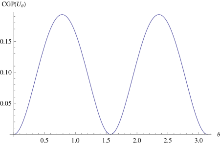
Figure 1: The coherence generating power of $U_{\theta}$ vs $\theta$

.

As a demonstration, we plot the $\mathrm{C}\mathrm{G}\mathrm{P}(U_{\theta})$ as the function of $\theta\in[0,\pi]$. From Fig. 1, we see that the coherence generating power of $U_{\theta}$ is a periodic function of $\theta$. In particular, the maximal CGP for $U_{\theta}$ is $\ln N-H_{N}+1=\ln 2-1/2=0.193$. We also see that the maximal CGP of $U_{\theta}$ is attained at $\theta=\pi/4$ and $3\pi/4$.

Example 4.3 (Square root of swap gate).

The $\sqrt{\text{swap}}$ gate is universal in the sense that any quantum multi-qubit gates can be constructed from $\sqrt{\text{swap}}$ and single qubit gates,

$$\sqrt{\text{swap}}=\left[\begin{array}[]{cccc}1&0&0&0\\ 0&\frac{1}{2}(1+\mathrm{i})&\frac{1}{2}(1-\mathrm{i})&0\\ 0&\frac{1}{2}(1-\mathrm{i})&\frac{1}{2}(1+\mathrm{i})&0\\ 0&0&0&1\end{array}\right].$$

By direct computation we have

$$\mathbf{C}\mathbf{G}\mathbf{P}(\sqrt{\text{swap}})=\frac{1}{2}\ln 2.$$

Example 4.4.

For a partial swap operator [41], one has $U_{t}\in\mathcal{U}(\mathbb{C}^{d}\otimes\mathbb{C}^{d})$: $U_{t}=\sqrt{t}\mathbb{I}_{d}\otimes\mathbb{I}_{d}+\mathrm{i}\sqrt{1-t}\,S$, where $S=\sum^{d}_{i,j=1}|ij\rangle\langle ji|$ and $t\in[0,1]$. In particular, for $d=2$, we have

$$U_{t}=\left[\begin{array}[]{cccc}\sqrt{t}+\sqrt{1-t}\mathrm{i}&0&0&0\\ 0&\sqrt{t}&\sqrt{1-t}\mathrm{i}&0\\ 0&\sqrt{1-t}\mathrm{i}&\sqrt{t}&0\\ 0&0&0&\sqrt{t}+\sqrt{1-t}\mathrm{i}\end{array}\right].$$

Then

$$B(U_{t})=U_{t}\star\overline{U}_{t}=\left[\begin{array}[]{cccc}1&0&0&0\\ 0&t&1-t&0\\ 0&1-t&t&0\\ 0&0&0&1\end{array}\right]$$

and

$$\mathbf{C}\mathbf{G}\mathbf{P}(U_{t})=\frac{t^{2}\ln t-(1-t)^{2}\ln(1-t)}{2(1-2t)},\quad t\in[0,1].$$

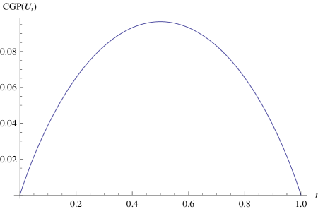
Figure 2: The coherence generating power of $U_{t}$

Again, we plot the $\mathbf{C}\mathbf{G}\mathbf{P}(U_{t})$ as the function of $t\in[0,1]$. From Fig. 2, we see that the maximal CGP of $U_{t}$, attained at $t=0.5$, is given by $\mathbf{C}\mathbf{G}\mathbf{P}(U_{1/2})=\frac{1}{4}(2\ln 2-1)=0.097$, which is less than the maximal CGP, $\ln 4-H_{4}+1=\ln 4-1/2-1/3-1/4=0.303$, of $4\times 4$ unitary matrices.

5 Conclusion

Based on probabilistic averages, we have defined a measure of the coherence generating power of a unitary operation: the average coherence generated by the unitary channel acting on a uniform ensemble of incoherent states. We have presented the explicit analytical formula of CGP for any unitary channel and any finite dimensions in terms of subentropy. An upper bound for CGP of a unital quantum channel has been also derived. Detailed examples have been studied.

We remark that Zanardi et al. [34, 35] studied the cohering and de-cohering power for unitary gates, based on the coherence measure of Hilbert-Schmidt norm, which is not really a well-defined measure of coherence. And their method is only suitable for unital quantum channels since the Hilbert-Schmidt norm is non-increasing under unital quantum channels. Hence the related computation is relatively easy as it involves only integrals in uniform Haar measure over pure states. In this work we used the bona fide coherence measure of relative entropy. Our approach applies to any quantum channels. The related computation concerns complex integral techniques with Dirac delta function and its Fourier integral representations. In addition, the formula in [34, 35] for CGP of unitary channels strongly depends on the dimension: the CGP approaches to zero when the dimension increases. However, our CGP of any unitary channels does not always approach to zero when the dimension goes to infinite. It is generally very difficult to compute the CGP for generic quantum channels. Our approach may highlight further researches on such characterization of quantum coherence.

Acknowledgements

This research was supported by Zhejiang Provincial Natural Science Foundation of China under Grant No. LY17A010027 and NSFC (Nos.11301124, 61771174), and also supported by the cross-disciplinary innovation team building project of Hangzhou Dianzi University. Other authors acknowledge supports from NSFC Grant Nos. 11275131, 11571313 (ZM); No.11571313(ZC); No. 11675113(SF). Huangjun Zhu is acknowledged for helpful discussions.

Appendix A: About the proof of the Theorem

We first introduce the following Lemma.

Lemma 5.1 (Jordan lemma).

Let $f(z)$ be analytic in the upper half-plane $\mathrm{Im}(z)\geqslant 0$, except for a finite number of isolated points. Let also $C_{R}$ be an arc of a semicircle $\left\lvert\mspace{1.0mu}z\mspace{1.0mu}\right\rvert=R$ in the upper half-plane. If for each $z$ on $C_{R}$, there is some constant $K_{R}$ such that $\left\lvert\mspace{1.0mu}f(z)\mspace{1.0mu}\right\rvert\leqslant K_{R}$ and $K_{R}\to 0$ as $R\to\infty$, then for $a>0$

$$\lim_{R\to\infty}\int_{C_{R}}e^{\mathrm{i}az}f(z)\mathrm{d}z=0.$$ (5.1)

Proof.

Set $z=Re^{\mathrm{i}\theta}$ and take into account that $\sin\theta\geqslant\frac{2}{\pi}\theta$ for $0\leqslant\theta\leqslant\frac{\pi}{2}$. We have that, if $R\to\infty$,

$$\left\lvert\mspace{1.0mu}\int_{C_{R}}e^{\mathrm{i}az}f(z)\mathrm{d}z\mspace{1.0mu}\right\rvert \leqslant K_{R}\cdot R\cdot\int^{\pi}_{0}e^{-aR\sin\theta}\mathrm{d}\theta$$

$$\leqslant K_{R}\frac{\pi}{a}\left(1-e^{-aR}\right)\to 0.$$

This completes the proof. ∎

If $a<0$ and $f(z)$ satisfies the conditions of Jordan lemma at $\mathrm{Im}(z)\leqslant 0$, the formula is still valid but at the integration over the arc $C_{R}$ in the lower half-plane. Similar statements take place at $a=\pm\mathrm{i}\alpha(\alpha>0)$ if the $C_{R}$-integration occurs in the right $(\Re(z)\geqslant 0)$ or left $(\Re(z)\leqslant 0)$ half-plane, respectively.

Now we prove the following two formulae used in the proof of the Theorem 3.1.

(i).

$$\mathcal{I}_{p}(\alpha)=\frac{\Gamma(N)\Gamma(1-\alpha-N)}{\Gamma(-\alpha)}\sum^{N}_{j=1}\frac{p^{\alpha+N-1}_{j}}{\prod_{i\neq j}(p_{i}-p_{j})},$$ (5.2)

(ii).

$$\mathcal{I}^{\prime}_{p}(1)=-\frac{1}{N}\left(H_{N}-1+\mathbf{Q}(p)\right),$$ (5.3)

where $\mathcal{I}_{p}(\alpha)$ is given by (3.3).

Proof.

(i). From the Fourier transform of the Dirac delta function $\delta$,

$$\delta\left(1-\sum^{N}_{j=1}\lambda_{j}\right)=\frac{1}{2\pi}\int^{\infty}_{-\infty}\exp\left(\mathrm{i}t\left(1-\sum^{N}_{j=1}\lambda_{j}\right)\right)\mathrm{d}t,$$ (5.4)

and the definition of Gamma function,

$$\left(\sum^{N}_{j=1}p_{j}\lambda_{j}\right)^{\alpha}=\frac{1}{\Gamma(-\alpha)}\int^{\infty}_{0}s^{-\alpha-1}\exp\left(-s\left(\sum^{N}_{j=1}p_{j}\lambda_{j}\right)\right)\mathrm{d}s,$$ (5.5)

we have

$$\mathcal{I}_{p}(\alpha) = \Gamma(N)\int^{\infty}_{0}\cdots\int^{\infty}_{0}\left(\sum^{N}_{j=1}p_{j}\lambda_{j}\right)^{\alpha}\delta\left(1-\sum^{N}_{j=1}\lambda_{j}\right)\prod^{N}_{k=1}\mathrm{d}\lambda_{k}$$ (5.6)

$$= \frac{\Gamma(N)}{2\pi\Gamma(-\alpha)}\int^{\infty}_{0}\frac{\mathrm{d}s}{s^{\alpha+1}}\int^{\infty}_{-\infty}\mathrm{d}t\cdot e^{\mathrm{i}t}\left[\int^{\infty}_{0}\cdots\int^{\infty}_{0}\prod^{N}_{k=1}\mathrm{d}\lambda_{k}\nabla_{1}\nabla_{2}\right],$$ (5.7)

where $\nabla_{1}=\exp\left(-s\left(\sum^{N}_{j=1}p_{j}\lambda_{j}\right)\right)$ and $\nabla_{2}=\exp\left(-\mathrm{i}t\sum^{N}_{j=1}\lambda_{j}\right)$. Substituting $f(x)=e^{-ax}H(x)$, where $H(x)=1_{(0,\infty)}$ is the Heaviside step function and $a>0$, into the following formula,

$$\widehat{f}(\omega)=\frac{1}{\sqrt{2\pi}}\int^{\infty}_{-\infty}f(x)e^{-\mathrm{i}\omega x}\mathrm{d}x,$$ (5.8)

we obtain that

$$\int^{\infty}_{0}e^{-ax}e^{-\mathrm{i}\omega x}\mathrm{d}x=\int^{\infty}_{-\infty}e^{-ax}H(x)e^{-\mathrm{i}\omega x}\mathrm{d}x=\frac{1}{\mathrm{i}\omega+a}.$$ (5.9)

Therefore

$$\int^{\infty}_{0}\cdots\int^{\infty}_{0}\prod^{N}_{k=1}\mathrm{d}\lambda_{k}\exp\left(-s\left(\sum^{N}_{j=1}p_{j}\lambda_{j}\right)\right)\exp\left(-\mathrm{i}t\sum^{N}_{j=1}\lambda_{j}\right)$$

$$=\prod^{N}_{j=1}\int^{\infty}_{0}\mathrm{d}\lambda_{j}e^{-sp_{j}\lambda_{j}}e^{-\mathrm{i}t\lambda_{j}}=\frac{1}{\prod^{N}_{j=1}(\mathrm{i}t+sp_{j})}.$$ (5.10)

It follows that

$$\mathcal{I}_{p}(\alpha)=\frac{\Gamma(N)}{2\pi\Gamma(-\alpha)}\int^{\infty}_{0}\frac{\mathrm{d}s}{s^{\alpha+1}}\left\{\int^{\infty}_{-\infty}\frac{e^{\mathrm{i}t}}{\prod^{N}_{j=1}(\mathrm{i}t+sp_{j})}\mathrm{d}t\right\}.$$ (5.11)

By using complex integral techniques in Lemma 5.1, we get

$$\int^{\infty}_{-\infty}\frac{e^{\mathrm{i}t}}{\prod^{N}_{j=1}(\mathrm{i}t+sp_{j})}\mathrm{d}t=\frac{2\pi}{s^{N-1}}\sum^{N}_{j=1}\frac{e^{-sp_{j}}}{\prod_{i\neq j}(p_{i}-p_{j})},$$ (5.12)

which gives rise to

$$\mathcal{I}_{p}(\alpha) = \frac{\Gamma(N)}{\Gamma(-\alpha)}\int^{\infty}_{0}\frac{\mathrm{d}s}{s^{\alpha+N}}\sum^{N}_{j=1}\frac{e^{-sp_{j}}}{\prod_{i\neq j}(p_{i}-p_{j})}$$ (5.13)

$$= \frac{\Gamma(N)}{\Gamma(-\alpha)}\sum^{N}_{j=1}\frac{1}{\prod_{i\neq j}(p_{i}-p_{j})}\int^{\infty}_{0}s^{-\alpha-N}e^{-sp_{j}}\mathrm{d}s$$ (5.14)

$$= \frac{\Gamma(N)\Gamma(1-\alpha-N)}{\Gamma(-\alpha)}\sum^{N}_{j=1}\frac{p^{\alpha+N-1}_{j}}{\prod_{i\neq j}(p_{i}-p_{j})}.$$ (5.15)

(ii). From the property of the Gamma function:

$$\Gamma(1-z)\Gamma(z)=\frac{\pi}{\sin(\pi z)},$$ (5.16)

we have

$$\Gamma(1-\alpha-N)=\frac{\pi}{\Gamma(\alpha+N)\sin(\alpha\pi+N\pi)}$$ (5.17)

and

$$\Gamma(-\alpha)=\frac{\pi}{\Gamma(\alpha+1)\sin(\alpha\pi+\pi)}.$$ (5.18)

Therefore $\mathcal{I}_{p}(\alpha)$ can be rewritten as

$$\mathcal{I}_{p}(\alpha) = \frac{\Gamma(N)\Gamma(\alpha+1)}{\Gamma(\alpha+N)}\frac{\sin(\alpha\pi+N\pi)}{\sin(\alpha\pi+\pi)}\sum^{N}_{j=1}\frac{p^{\alpha+N-1}_{j}}{\prod_{i\neq j}(p_{i}-p_{j})}$$ (5.19)

$$= (-1)^{N-1}\frac{\Gamma(N)\Gamma(\alpha+1)}{\Gamma(\alpha+N)}\sum^{N}_{j=1}\frac{p^{\alpha+N-1}_{j}}{\prod_{i\neq j}(p_{i}-p_{j})},$$ (5.20)

which gives rise to

$$\mathcal{I}_{p}(\alpha)=\frac{\Gamma(N)\Gamma(\alpha+1)}{\Gamma(\alpha+N)}\sum^{N}_{j=1}\frac{p^{\alpha+N-1}_{j}}{\prod_{i\neq j}(p_{j}-p_{i})}.$$ (5.21)

Taking the derivative of $\mathcal{I}_{p}(\alpha)$ with respect to $\alpha$, we get

$$\mathcal{I}^{\prime}_{p}(\alpha) = \displaystyle\Gamma(N)\frac{\mathrm{d}}{\mathrm{d}\alpha}\frac{\Gamma(\alpha+1)}{\Gamma(\alpha+N)}\sum^{N}_{j=1}\frac{p^{\alpha+N-1}_{j}}{\prod_{i\neq j}(p_{j}-p_{i})}$$ (5.22)

$$+\frac{\Gamma(N)\Gamma(\alpha+1)}{\Gamma(\alpha+N)}\sum^{N}_{j=1}\frac{p^{\alpha+N-1}_{j}\ln p_{j}}{\prod_{i\neq j}(p_{j}-p_{i})}.$$

This implies that, for $\alpha=1$,

$$\mathcal{I}^{\prime}_{p}(1)=\frac{1}{N}(\psi(2)-\psi(1+N))\sum^{N}_{j=1}\frac{p^{N}_{j}}{\prod_{i\neq j}(p_{j}-p_{i})}+\frac{1}{N}\sum^{N}_{j=1}\frac{p^{N}_{j}\ln p_{j}}{\prod_{i\neq j}(p_{j}-p_{i})},$$ (5.23)

where $\psi(2)=1-\gamma$, $\psi(1+N)=H_{N}-\gamma$, where $\gamma\simeq 0.57721$.

We compute the following summation in (5.23),

$$F(p_{1},\ldots,p_{N}):=\sum^{N}_{j=1}\frac{p^{N}_{j}}{\prod_{i\neq j}(p_{j}-p_{i})}.$$ (5.24)

Since it is a rational symmetric function, homogeneous of degree one, with all singularities removable, it must be a multiple of $\sum^{N}_{j=1}p_{j}$. That is, $F(tp_{1},\ldots,tp_{N})=tF(p_{1},\ldots,p_{N})$ for any real number $t$, and $F(p_{\sigma(1)},\ldots,p_{\sigma(N)})=F(p_{1},\ldots,p_{N})$ for all permutations $\sigma\in S_{N}$. This means that

$$F(p_{1},\ldots,p_{N})\propto\sum^{N}_{j=1}p_{j}.$$ (5.25)

Without loss of generality, assume that $F(p_{1},\ldots,p_{N})=C\cdot\sum^{N}_{j=1}p_{j}$ for some constant $C$. By setting $(p_{1},\ldots,p_{N})=(1,0,\ldots,0)$, we get $C=1$. That is,

$$\sum^{N}_{j=1}\frac{p^{N}_{j}}{\prod_{i\neq j}(p_{j}-p_{i})}=\sum^{N}_{j=1}p_{j}=1.$$ (5.26)

Therefore, from (2.4), (5.23) gives rise to

$$-N\cdot\mathcal{I}^{\prime}_{p}(1) = \displaystyle(\psi(1+N)-\psi(2))\sum^{N}_{j=1}\frac{p^{N}_{j}}{\prod_{i\neq j}(p_{j}-p_{i})}-\sum^{N}_{j=1}\frac{p^{N}_{j}\ln p_{j}}{\prod_{i\neq j}(p_{j}-p_{i})}$$ (5.27)

$$= H_{N}-1+\boldsymbol{Q}(p).$$ (5.28)

Hence $\mathcal{I}^{\prime}_{p}(1)=-\frac{1}{N}\left(H_{N}-1+\boldsymbol{Q}(p)\right)$. ∎

Appendix B: Proof of $\boldsymbol{Q}(B^{\scriptscriptstyle\mathsf{T}})\leqslant\boldsymbol{H}(B)$

To prove the relation $\boldsymbol{Q}(B^{\scriptscriptstyle\mathsf{T}})\leqslant\boldsymbol{H}(B)$, we prove that following relation first:

$$\Gamma(N)\int\boldsymbol{H}_{\lambda}(B)\delta\left(1-\sum^{N}_{i=1}\lambda_{i}\right)\prod^{N}_{j=1}\mathrm{d}\lambda_{j}=\frac{1}{N}\left(\sum^{N}_{i=1}\boldsymbol{H}(\beta_{i})\right).$$ (5.29)

Proof.

Since $\boldsymbol{H}(B\lambda)-\boldsymbol{H}(\lambda)\leqslant\boldsymbol{H}_{\lambda}(B)=\sum^{N}_{j=1}\lambda_{j}\boldsymbol{H}(\beta_{j})$, it follows that

$$\Gamma(N)\int\boldsymbol{H}_{\lambda}(B)\delta\left(1-\sum^{N}_{i=1}\lambda_{i}\right)\prod^{N}_{j=1}\mathrm{d}\lambda_{j}$$ (5.30)

$$=\Gamma(N)\int\left(\sum^{N}_{i=1}\lambda_{i}\boldsymbol{H}(\beta_{i})\right)\delta\left(1-\sum^{N}_{i=1}\lambda_{i}\right)\prod^{N}_{j=1}\mathrm{d}\lambda_{j}$$ (5.31)

$$=\Gamma(N)\sum^{N}_{i=1}\boldsymbol{H}(\beta_{i})\int\lambda_{i}\delta\left(1-\sum^{N}_{i=1}\lambda_{i}\right)\prod^{N}_{j=1}\mathrm{d}\lambda_{j}$$ (5.32)

$$=\left(\sum^{N}_{i=1}\boldsymbol{H}(\beta_{i})\right)\Gamma(N)\int\lambda_{1}\delta\left(1-\sum^{N}_{i=1}\lambda_{i}\right)\prod^{N}_{j=1}\mathrm{d}\lambda_{j}.$$ (5.33)

Denote

$$f(t)=\Gamma(N)\int\lambda_{1}\delta\left(t-\sum^{N}_{i=1}\lambda_{i}\right)\prod^{N}_{j=1}\mathrm{d}\lambda_{j}.$$ (5.34)

Performing Laplace transform ($t\to s$) of $f$, we obtain

$$\widetilde{f}(s)=\int^{\infty}_{0}f(t)e^{-st}\mathrm{d}t=\Gamma(N)\int\prod^{N}_{j=1}\mathrm{d}\lambda_{j}\left(\lambda_{1}\int^{\infty}_{0}\delta\left(t-\sum^{N}_{i=1}\lambda_{i}\right)e^{-st}\mathrm{d}t\right).$$ (5.35)

That is,

$$\widetilde{f}(s) = \Gamma(N)\int\prod^{N}_{j=1}\mathrm{d}\lambda_{j}\left(\lambda_{1}\int^{\infty}_{0}\delta\left(t-\sum^{N}_{i=1}\lambda_{i}\right)e^{-st}\mathrm{d}t\right)$$ (5.36)

$$= \Gamma(N)\int\prod^{N}_{j=1}\mathrm{d}\lambda_{j}\lambda_{1}e^{-s\sum^{N}_{i=1}\lambda_{i}}$$ (5.37)

$$= \Gamma(N)\int\lambda_{1}e^{-s\lambda_{1}}\mathrm{d}\lambda_{1}\times\int e^{-s\lambda_{2}}\mathrm{d}\lambda_{2}\times\cdots\times\int e^{-s\lambda_{N}}\mathrm{d}\lambda_{N}$$ (5.38)

$$= \Gamma(N)s^{-N-1}\int^{\infty}_{0}xe^{-x}\mathrm{d}x=\frac{\Gamma(N)}{s^{N+1}}.$$ (5.39)

Thus $f(t)=\frac{1}{N}t^{N}$. Therefore

$$\Gamma(N)\int\boldsymbol{H}_{\lambda}(B)\delta\left(1-\sum^{N}_{i=1}\lambda_{i}\right)\prod^{N}_{j=1}\mathrm{d}\lambda_{j}=\frac{1}{N}\left(\sum^{N}_{i=1}\boldsymbol{H}(\beta_{i})\right).$$ (5.40)

We have done. ∎

As a by-product of the formula (5.29), we have $\boldsymbol{Q}(B^{\scriptscriptstyle\mathsf{T}})\leqslant\boldsymbol{H}(B)$.

References

- [1] L. Mandel and E. Wolf, Optical Coherence and Quantum Optics (Cambridge University Press, Cambridge, England, 1995).
- [2] F. London and H. London, Proc. R. Soc. A 149, 71 (1935).
- [3] P. Ćwikliński, M. Studziński, M. Horodecki, and J. Oppenheim, Phys. Rev. Lett. 115, 210403 (2015).
- [4] E. Bagan, J. A. Bergou, S. S. Cottrell, and M. Hillery, Phys. Rev. Lett. 116, 160406 (2016).
- [5] P. K. Jha, M. Mrejen, J. Kim, C. Wu, Y. Wang, Y. V. Rostovtsev, and X. Zhang, Phys. Rev. Lett. 116, 165502 (2016).
- [6] P. Kammerlander and J. Anders, Sci. Rep. 6, 22174 (2016).
- [7] H. L. Shi, S. Y. Liu, X. H. Wang, W. L. Yang, Z. Y. Yang, H. Fan, Phys. Rev. A 95, 032307 (2017).
- [8] S. Lloyd, J.Phys.: Conf. Ser. 302, 012037 (2011).
- [9] C. M. Li, N. Lambert, Y. N. Chen, G. Y. Chen, and F. Nori, Sci. Rep. 2, 885 (2012).
- [10] S. Huelga and M. Plenio, Contemporary Physics 54, 181 (2013).
- [11] V. Singh Poonia, D. Saha, and S. Ganguly, arXiv:1408.1327, (2014).
- [12] T. Baumgratz, M. Cramer, and M. B. Plenio, Phys. Rev. Lett. 113, 140401 (2014).
- [13] T. Theurer, N. Killoran, D. Egloff, and M.B. Plenio, Phys. Rev. Lett. 119, 230401 (2017).
- [14] J. Aberg, arXiv:quant-ph/0612146
- [15] A. Winter and D. Yang, Phys. Rev. Lett. 116, 120404 (2016).
- [16] S. Cheng and M. J. W. Hall, Phys. Rev. A 92, 042101 (2015).
- [17] C. Napoli, T. R. Bromley, M. Cianciaruso, M. Piani, N. Johnston, and G. Adesso, Phys. Rev. Lett. 116, 150502 (2016).
- [18] U. Singh, L. Zhang, and A. K. Pati, Phys. Rev. A 93, 032125 (2016).
- [19] L. Zhang, U. Singh, A.K. Pati, Ann. Phys. 377, 125-146 (2017).
- [20] K. Bu, U. Singh, S-M. Fei, A. K. Pati, J. Wu, Phys. Rev. Lett. 119, 150405 (2017).
- [21] I. Marvian and R.W. Spekkens, Phys. Rev. A 94, 052324 (2016).
- [22] M. Piani, M. Cianciaruso, T. R. Bromley, C. Napoli, N. Johnston, and G. Adesso, Phys. Rev. A 93, 042107 (2016).
- [23] I. Marvian, R. W. Spekkens, and P. Zanardi, Phys. Rev. A 93, 052331 (2016).
- [24] A. Streltsov, U. Singh, H. S. Dhar, M. N. Bera, and G. Adesso, Phys. Rev. Lett. 115, 020403 (2015).
- [25] C. Radhakrishnan, M. Parthasarathy, S. Jambulingam, and T. Byrnes, Phys. Rev. Lett. 116, 150504 (2016).
- [26] J. Ma, B. Yadin, D. Girolami, V. Vedral, and M. Gu, Phys. Rev. Lett. 116, 160407 (2016).
- [27] G. Karpat, B. Cakmak, and F. F. Fanchini, Phys. Rev. B 90, 104431 (2014).
- [28] A. L. Malvezzi, G. Karpat, B. Cakmak, F. F. Fanchini, T. Debarba, and R. O. Vianna, Phys. Rev. B 93, 184428 (2016).
- [29] E. Chitambar, M. H. Hsieh, Phys. Rev. Lett. 117, 020402 (2016).
- [30] H. J. Zhu, Z. H. Ma, Z. Cao, S. M. Fei, V. Vedral, Phys. Rev. A 96, 032316 (2017).
- [31] A. Mani and V. Karimipour, Phys. Rev. A 92, 032331 (2015).
- [32] A. Misra, U. Singh, S. Bhattacharya, and A. K. Pati, Phys. Rev. A 93, 052335 (2016).
- [33] M. G. Díaz, D. Egloff, M.B. Plenio, Quant. Inf. Comput. 16, 1282-1294 (2016).
- [34] P. Zanardi, G. Styliaris, and L.C. Venuti, Phys. Rev. A 95, 052306(2017).
- [35] P. Zanardi, G. Styliaris, and L. C. Venuti, Phys. Rev. A 95, 052307 (2017).
- [36] L. Zhang and J. Wu, Phys. Lett. A 375, 4163-4165 (2011).
- [37] A. Lasota and M.C. Mackey, Chaos, Fractals, and Noise. Stochastic Aspects of Dynamics, Springer-Verlag, New York (1994).
- [38] D.N. Page, Phys. Rev. Lett. 71, 1291 (1993).
- [39] L. Zhang, J. Phys. A : Math. Theor. 50, 155303 (2017).
- [40] F. Buscemi, S. Das, M.M. Wilde, Phys. Rev. A 93, 062314 (2016).
- [41] K.M.R. Audenaert, N. Datta, M. Ozols, J. Math. Phys. 57, 052202 (2016).