Revisionist Simulations:
A New Approach to Proving Space Lower Bounds

Abstract

Determining the number of registers required for solving $x$-obstruction-free (or randomized wait-free) $k$-set agreement for $x\leq k$ is an open problem that highlights important gaps in our understanding of the space complexity of synchronization. In $x$-obstruction-free protocols, processes are required to return in executions where at most $x$ processes take steps. The best known upper bound on the number of registers needed to solve this problem among $n>k$ processes is $n-k+x$ registers. No general lower bound better than $2$ was known.

We prove that any $x$-obstruction-free protocol solving $k$-set agreement among $n>k$ processes must use $\lfloor\frac{n-x}{k+1-x}\rfloor+1$ or more registers. Our main tool is a simulation that serves as a reduction from the impossibility of deterministic wait-free $k$-set agreement. In particular, we show that, if a protocol uses fewer registers, then it is possible for $k+1$ processes to simulate the protocol and deterministically solve $k$-set agreement in a wait-free manner, which is impossible.

We generalize this simulation to prove space lower bounds for $x$-obstruction-free protocols solving colorless tasks. In particular, we prove a lower bound of $\lfloor\frac{n}{2}\rfloor+1$ for obstruction-free $\epsilon$-approximate agreement, for sufficiently small $\epsilon$. An important aspect of the simulation is the ability of simulating processes to revise the past of simulated processes. We introduce an augmented snapshot object, which facilitates this.

We also prove that any lower bound on the number of registers used by obstruction-free protocols applies to protocols that satisfy nondeterministic solo termination. Hence, our lower bounds for the obstruction-free case also holds for randomized wait-free protocols. In particular, we get a tight lower bound of exactly $n$ registers for solving obstruction-free and randomized wait-free consensus.

He who controls the past controls the future. He who controls the present controls the past.

George Orwell, 1984

1 Introduction

The $k$-set agreement problem, introduced by Chaudhuri [19], is a well-known synchronization task in which $n>k$ processes, each with an input value, are required to output at most different $k$ values, each of which is the input of some process. This is a generalization of the classical consensus problem, which is the case $k=1$.

Two celebrated results in distributed computing are the impossibility of solving consensus deterministically when at most one process may crash [25, 38] and, more generally, the impossibility of solving $k$-set agreement deterministically when at most $k$ processes may crash [14, 34, 41], using only registers. One way to bypass these impossibility results is to design protocols that are obstruction-free [33]. Obstruction-freedom is a termination condition that requires a process to terminate given sufficiently many consecutive steps, i.e., from any configuration, if only one process takes steps, then it will eventually terminate. $x$-obstruction-freedom [45] generalizes this condition: from any configuration, if only $x$ processes take steps, then they will all eventually terminate. It is known that $k$-set agreement can be solved using only registers in an $x$-obstruction-free way for $1\leq x\leq k$  [46]. Another way to overcome the impossibility of solving consensus is to use randomized wait-free protocols, where non-faulty processes are required to terminate with probability $1$ [13].

It is possible to solve consensus for $n$ processes using $n$ registers in a randomized wait-free way [1, 3, 40, 5] or in an obstruction-free way [30, 17, 47, 16]. A lower bound of $\Omega(\sqrt{n})$ was proved by Ellen, Herlihy, and Shavit in [23]. Recently, Gelashvili proved an $\Omega(n)$ lower bound for anonymous processes [28]. Anonymous processes [23, 7] have no identifiers and run the same code: all processes with the same input start in the same initial state and behave identically until they read different values. Then Zhu proved that any obstruction-free protocol solving consensus for $n$ processes requires at least $n-1$ registers [48]. All these lower bounds are actually for protocols that satisfy nondeterministic solo termination [23], which includes both obstruction-free and randomized wait-free protocols.

In contrast, there are big gaps between the best known upper and lower bounds on the number of registers needed for $k$-set agreement. The best obstruction-free protocols require $n-k+1$ registers [47, 16]. Bouzid, Raynal, and Sutra [16] also give an $x$-obstruction-free protocol that uses $n-k+x$ registers, improving on the $min(n+2x-k,n)$ space complexity of Delporte-Gallet, Fauconnier, Gafni, and Rajsbaum’s obstruction-free protocol [20]. All of these algorithms work for anonymous processes. Delporte-Gallet, Fauconnier, Kuznetsov, and Ruppert [21] proved that it is impossible to solve $k$-set agreement using $1$ register. For anonymous processes, they also proved a lower bound of $\sqrt{x(\frac{n}{k}-2)}$ for $x$-obstruction-free protocols, which still leaves a polynomial gap between the lower and upper bounds.

There are good reasons why proving lower bounds on the number of registers needed for $k$-set agreement may be difficult. At a high level, the impossibility results for $k$-set agreement consider some representation (for example, a simplicial complex) of all possible process states in all possible executions. Then, a combinatorial property (Sperner’s Lemma [44]) is used to prove that, roughly speaking, for any given number of steps, there exists an execution leading to a configuration in which $k+1$ outputs are still possible. Although there is ongoing work to develop a more general theory [27, 42, 26], we do not know enough about the topological representation of protocols that are $x$-obstruction-free or use fewer than $n$ multi-writer registers [32] to adapt topological arguments to prove space lower bounds for $k$-set agreement. There are similar problems adapting known proofs that do not explicitly use topology [4, 10].

Approximate agreement [22] is another important task for which no good space lower bound was known. In $\epsilon$-approximate agreement, each process starts with an input in $\{0,1\}$. The processes are required to output values in the interval $[0,1]$ that are all within $\epsilon$ of each other. Moreover, each output value must lie between the smallest input and the largest input. This problem can be deterministically solved in a wait-free manner, i.e. every non-faulty process eventually outputs a value. The only space lower bound for this problem, $\Omega(\log(\frac{1}{\epsilon}))$, was in a restricted setting with single-bit registers [43]. The best upper bounds are $\lceil\log_{2}(\frac{1}{\epsilon})\rceil$ [43] and $n$ [9].

Our contribution. In this paper, we prove a lower bound of $\lfloor\frac{n-x}{k+1-x}\rfloor+1$ on the number of registers necessary for solving $n$-process $x$-obstruction-free $k$-set agreement. As corollaries, we get a tight lower bound of $n$ registers for obstruction-free consensus and a tight lower bound of 2 for obstruction-free $(n-1)$-set consensus. We also prove a space lower bound of $\lfloor\frac{n}{2}\rfloor+1$ registers for obstruction-free $\epsilon$-approximate agreement, for sufficiently small $\epsilon$. More generally, we prove space lower bounds for colorless tasks.

In addition, in Section 5, we prove that any lower bound on the number registers needed for obstruction-free protocols to solve a task also applies to nondeterministic solo terminating protocols and, in particular, to randomized wait-free protocols solving that task. Hence, our space lower bounds for obstruction-free protocols also apply to such protocols. We also show that the same result may be obtained for a large class of objects.

Technical Overview. Using a novel simulation, we convert any obstruction-free protocol for $k$-set agreement that uses too few registers to a protocol that solves wait-free $k$-set agreement using only registers. Since solving wait-free $k$-set agreement is impossible using only registers, this reduction gives a lower bound on the number of registers needed to solve obstruction-free $k$-set agreement. This simulation technique, described in detail in Section 4, is the main technical contribution of the paper. It is the first technique that proves lower bounds on space complexity by applying results obtained by topological arguments. We also use this new technique to prove a lower bound on the number of registers needed for $\epsilon$-approximate agreement by a reduction from a step complexity lower bound for $\epsilon$-approximate agreement. Specifically, we convert any obstruction-free protocol for $\epsilon$-approximate agreement to a protocol that uses few registers to a protocol that solves $\epsilon$-approximate agreement for two processes such that both processes take few steps.

The executions of the simulated processes in our simulation are reminiscent of the executions constructed by adversaries in covering arguments [18, 6]. In those proofs, the adversary modifies an execution it has constructed by revising the past of some process, so that the old and new executions are indistinguishable to the other processes. It does so by inserting consecutive steps of the process starting from some carefully chosen configuration. In our simulation, a real process may revise the past of a simulated process, in a way that is indistinguishable to other simulated processes. This is possible because each simulated process is simulated by a single real process. In contrast, in the BG simulation [15], different steps of simulated processes can be performed by different real processes, so this would be much more difficult to do.

A crucial component of our simulation is the use of an augmented snapshot object, which we implement in a non-blocking manner from registers. Like a standard snapshot object, this object consists of a fixed number of components and supports a $\mathord{\tt Scan}$ operation, which returns the contents of all components. However, it generalizes the $\mathord{\tt update}$ operation to a $\mathord{\tt Block-Update}$ operation, which can update multiple components of the object. In addition, a $\mathord{\tt Block-Update}$ returns some information, which is used by our simulation. The specifications of $\mathord{\tt Block-Update}$ and our implementation of an augmented snapshot object appears in Section 3.

2 Preliminaries

An asynchronous shared memory system consists of a set of processes and instances of base objects, which processes use to communicate. An object has a set of possible values and a set of operations, each of which takes some fixed number of inputs and returns a response. The processes take steps at arbitrary speeds and may fail, at any time, by crashing. Every step consists of an operation on some base object by some process plus local computation by that process to determine its next state from the response returned by the operation.

Configurations and Executions. A configuration of a system consists of the state of each process and the value of each object. An initial configuration is determined by the input value of each process. Each object has the same value in all initial configurations. A configuration $C$ is indistinguishable from a configuration $C^{\prime}$ to a set of processes $\mathcal{P}$ in the system, if every process in $\mathcal{P}$ is in the same state in $C$ as it is in $C^{\prime}$ and each object in the system has the same value in $C$ as in $C^{\prime}$.

A step $e$ by a process $p$ is applicable at a configuration $C$ if $e$ can be the next step of process $p$ given its state in $C$. If $e$ is applicable at $C$, then we use $Ce$ to denote the configuration resulting from $p$ taking step $e$ at $C$. A sequence of steps $\alpha=e_{1},e_{2},\dots$ is applicable at a configuration $C$ if $e_{1}$ is applicable at $C$ and, for each $i\geq 1$, $e_{i+1}$ is applicable at $Ce_{1}\cdots e_{i}$. In this case, $\alpha$ is called an execution from $C$. An execution $\alpha\beta$ denotes the execution $\alpha$ followed by the execution $\beta$. A configuration $C$ is reachable if there exists a finite execution from an initial configuration that results in $C$.

For a finite execution $\alpha$ from a configuration $C$, we use $C\alpha$ to denote the configuration reached after applying $\alpha$ to $C$. If $\alpha$ is empty, then $C\alpha=C$. We say an execution $\alpha$ is $\mathcal{P}$-only, for a set of processes $\mathcal{P}$, if all steps in $\alpha$ are by processes in $\mathcal{P}$. A $\{p\}$-only execution, for some process $p$, is also called a solo execution by $p$. Note, if configurations $C$ and $C^{\prime}$ are indistinguishable to a set of processes $\mathcal{P}$, then any $\mathcal{P}$-only execution from $C$ is applicable at $C^{\prime}$.

Implementations and Linearizability. An implementation of an object specifies, for each process and each operation of the object, a deterministic procedure describing how the process carries out the operation. The execution interval of an invocation of an operation in an execution is the subsequence of the execution that begins with its first step and ends with its last step. If an operation does not complete, for example, if the process that invoked it crashed before receiving a response, then its execution interval is infinite. An implementation of an object is linearizable if, for every execution, there is a point in each operation’s execution interval, called the linearization point of the operation, such that the operation can be said to have taken place atomically at that point [35]. This is equivalent to saying that the operations can be ordered (and all incomplete operations can be given responses) so that any operation which ends before another one begins is ordered earlier and the responses of the operations are consistent with the sequential specifications of the object [35].

Progress Conditions. An implementation of an object is wait-free if every process is able to complete its current operation on the object after taking sufficiently many steps, regardless of what other processes are doing. An implementation is non-blocking if infinitely many operations are completed in every infinite execution.

A protocol is $x$-obstruction-free if, from any configuration $C$ and for any subset $P$ of at most $x$ processes, every process in $P$ that takes sufficiently many steps after $C$ outputs a value, as long as only processes in $P$ take steps after $C$. A protocol is obstruction-free if it is 1-obstruction-free and wait-free if it is $n$-obstruction-free.

Registers and Snapshot objects. A register is an object that supports two operations, $\mathord{\tt write}$ and $\mathord{\tt read}$. A $\mathord{\tt write(v)}$ operation writes value $v$ to the register, and a $\mathord{\tt read}$ operation returns the last value that was written to the register before the read. A multi-writer register allows all processes to write to it, while a single-writer register can only be written to by one fixed process. A process is said to be covering a register if its next step is a write to this register. A block write is a consecutive sequence of $\mathord{\tt write}$ operations to different registers performed by different processes.

An $m$-component multi-writer snapshot object [2] stores a sequence of $m$ values and supports two operations, $\mathord{\tt update}$ and $\mathord{\tt scan}$. An $\mathord{\tt update}(j,v)$ operation sets component $j$ of the object to $v$. A $\mathord{\tt scan}$ operation returns the current view, consisting of the values of all components. A single-writer snapshot object shared by a set of processes has one component for each process and each process may only $\mathord{\tt update}$ its own component. A process is said to be covering component $j$ of a snapshot object if its next step is an update to the component $j$. A block update is a consecutive sequence of $\mathord{\tt update}$ operations to different components of a snapshot object performed by different processes.

It is easy to implement $m$ registers from an $m$-component multi-writer snapshot object, by replacing each $\mathord{\tt write}$ to the $j$’th register by an $\mathord{\tt update}$ to the $j$’th component and replacing a $\mathord{\tt read}$ to the $j$’th register by a $\mathord{\tt scan}$ and then discarding all but the value of the $j$’th component. An $m$-component snapshot object can also be implemented from $m$ registers [2].

Tasks and Protocols. A task specifies a set of allowable combinations of inputs to the processes and, for each such combination, what combinations of outputs can be returned by the processes. A protocol for a task provides a procedure for each process to compute its output, so that the task’s specifications are satisfied.

A task is colorless if the input or output of any process may be the input or output, respectively, of another process. Moreover, the specification of the task does not depend on the number of processes in the system. More precisely, a colorless task is a triple $(\mathcal{I},\mathcal{O},\Delta)$, where $\mathcal{I}$ contains sets of possible inputs, $\mathcal{O}$ contains sets of possible outputs, and, for each input set $I\in\mathcal{I}$, $\Delta(I)$ specifies a subset of $\mathcal{O}$, corresponding to valid outputs for $I$. Moreover, $\mathcal{I}$, $\mathcal{O}$, and $\Delta(I)$, for each $I\in\mathcal{I}$, are closed under taking subsets; i.e. if a set is present, then so are its non-empty subsets. The following are all examples of colorless tasks:

• Consensus: Each process begins with an arbitrary value as its input and, if it does not crash, must output a value such that no two processes output different values and each output value is the input of some process.

• $k$-Set agreement: Each process begins with an arbitrary value as its input and, if it does not crash, must output a value such that at most $k$ values are output and each output value is the input of some process.

• $\epsilon$-Approximate Agreement: Each process begins with an arbitrary (real) value as its input and, if it does not crash, must output a value such that any two output values are at most $\epsilon$ apart. Moreover, the set of output values is in the interval $[min,max]$, where $min$ and $max$ are the smallest and largest input values, respectively.

The space complexity of a protocol is the maximum number of registers used in any execution of the protocol. Each $m$-component snapshot object it uses counts as $m$ registers. The space complexity of a task is the minimum space complexity of any protocol for the task.

2.1 Our Setting

We consider two asynchronous shared memory systems, the simulated system and the real system.

Simulated system. The simulated system consists of $n$ simulated processes, $p_{1},\ldots,p_{n}$, that communicate through an $m$-component multi-writer snapshot object. Thus, any task that can be solved in the simulated system has space complexity at most $m$.

Without loss of generality, we assume that each process $p_{i}$ alternately performs $\mathord{\tt scan}$ and $\mathord{\tt update}$ operations on the snapshot object: Between two consecutive $\mathord{\tt update}$ operations, $p_{i}$ can perform a $\mathord{\tt scan}$ and ignore its result. If $p_{i}$ is supposed to perform multiple consecutive $\mathord{\tt scan}$s, it can, instead, perform one $\mathord{\tt scan}$ and use its result as the result of the others. This is because it is possible for all these $\mathord{\tt scan}$s to occur consecutively in an execution, in which case, they would all get the same result.

Real system. The real system consists of $f$ real processes, $q_{1},\ldots,q_{f}$, that communicate through a single-writer snapshot object. For clarity of presentation, real processes use single-writer registers in addition to the single-writer snapshot object. The single-writer registers to which a particular process writes can be treated as additional separate fields of the component of the snapshot object belonging to that process. In Section 3, we define and implement an $m$-component augmented snapshot object shared by the real processes.

In our simulation, the processes in the simulated system are partitioned into $f$ sets, $P_{1},\ldots,P_{f}$, and real process $q_{i}$ is solely responsible for simulating the actions of all processes in $P_{i}$ in the simulated system. This is illustrated in Figure 1.

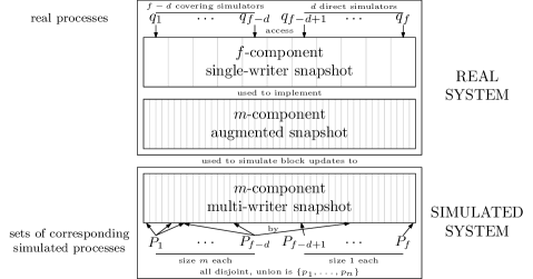
Figure 1: High-level overview of real and simulated systems.

3 Augmented Snapshot Object

In this section, we define an augmented snapshot object and show how it can be deterministically implemented in the real system. This object plays a central role in our simulation. It is used by real processes to simulate steps performed by simulated processes. In particular, a real process $q_{i}$ uses this object to simulate an $\mathord{\tt update}$ or a $\mathord{\tt scan}$ by any simulated process in $P_{i}$, or a block update by any subset of processes in $P_{i}$. Our simulation, which is explained in Section 4, is non-standard. Unfortunately, to satisfy its technical requirements, the augmented snapshot has to satisfy some non-standard properties.

An $m$-component augmented snapshot object is a generalization of an $m$-component multi-writer snapshot object. A $\mathord{\tt Scan}$ operation returns the current view, consisting of the values of all components. The components can be updated using a $\mathord{\tt Block-Update}$ operation. The key difference between a multi-writer snapshot and an augmented snapshot is that a $\mathord{\tt Block-Update}$ may update multiple components, although not necessarily atomically. In addition, a $\mathord{\tt Block-Update}$ may return a view from some earlier point in the execution. Otherwise, it returns a special yield symbol, .

A linearizable, non-blocking implementation of an augmented snapshot object in the real system is impossible. This is because a $\mathord{\tt Block-Update}$ operation that updates 2 components would then be the same as a $\mathord{\tt 2-assignment}$ operation. However, $\mathord{\tt 2-assignment}$, together with $\mathord{\tt read}$ or $\mathord{\tt Scan}$, can be used to deterministically solve wait-free consensus among 2 processes [31], which is impossible in the real system [2, 38].

Instead, a $\mathord{\tt Block-Update}$ operation can be considered to be a sequence of atomic $\mathord{\tt Update}$ operations, which each update one component of the augmented snapshot object. (Analogously, a collect operation [12, 9] is not atomic, but the individual reads that comprise it are atomic.)

3.1 Specification

An $m$-component augmented snapshot object, $\mathcal{M}[1..m]$, shared by $f$ processes, $q_{1},\dots,q_{f}$, consists of $m$ components and supports two operations, $\mathord{\tt Scan}$ and $\mathord{\tt Block-Update}$, which can be performed by all processes. A view of the augmented snapshot consists of the value of each of the $m$ components at some point in an execution. A $\mathord{\tt Scan}$ operation returns the current view. A $\mathord{\tt Block-Update}$ operation to a sequence of $r\geq 1$ different components $[j_{1},\dots,j_{r}]$ of $\mathcal{M}$ with a sequence of $r$ values $[v_{1},\dots,v_{r}]$ is comprised of a sequence of $\mathord{\tt Update}$ operations $U_{1},\dots,U_{r}$. Each $\mathord{\tt Update}$ $U_{g}$ atomically sets $\mathcal{M}[j_{g}]$ to $v_{g}$. These $\mathord{\tt Update}$ operations may occur in any order. A $\mathord{\tt Block-Update}$ operation also returns either or a view of $\mathcal{M}$.

A $\mathord{\tt Block-Update}$ that does not return is called atomic. We require that every execution has a linearization in which the $\mathord{\tt Update}$ operations comprising each atomic $\mathord{\tt Block-Update}$ are linearized consecutively.

Consider any atomic $\mathord{\tt Block-Update}$, $B$. Let $Z$ be the first $\mathord{\tt Update}$ in $B$. Let $Z^{\prime}$ be the last $\mathord{\tt Update}$ prior to $Z$ that is part of an atomic $\mathord{\tt Block-Update}$ or the beginning of the execution, if there is no such $\mathord{\tt Update}$. Then $B$ must return a view of $\mathcal{M}$ at some point $T$ between $Z^{\prime}$ and $Z$ such that no $\mathord{\tt Scan}$ occurs between $T$ and $Z$.

We prove that, in our implementation, a $\mathord{\tt Block-Update}$ only returns under certain circumstances, as described in Theorem 20. For example, a $\mathord{\tt Block-Update}$ by process $q_{1}$ will always be atomic and, if a $\mathord{\tt Block-Update}$ experiences no step contention [8], it will be atomic. The simulation in Section 4 relies on this property of our implementation.

3.2 Implementation

In this section, we describe how to implement an $m$-component augmented snapshot object, $\mathcal{M}$, shared by $f$ processes, $q_{1},\dots,q_{f}$, in the real system. Our implementation is non-blocking: every $\mathord{\tt Block-Update}$ operation is wait-free, while a $\mathord{\tt Scan}$ operation can only be blocked by an infinite sequence of concurrent $\mathord{\tt Block-Update}$ operations.

The implementation uses a shared single-writer snapshot object $\mathsf{H}[1..f]$. All $f$ components of $\mathsf{H}$ are initially $\bot$. The $i$’th component of $\mathsf{H}$ is used by $q_{i}$ to record a list of every $\mathord{\tt Update}$ it performs, each represented by a triple. A triple contains a component of $\mathcal{M}$, a value, and a timestamp. Each time $q_{i}$ performs a $\mathord{\tt Block-Update}$ to $r$ components of $\mathcal{M}$, it appends $r$ triples to $\mathsf{H}[i]$, all with the same timestamp. For clarity of presentation, we also use $n(n-1)$ unbounded arrays of single-writer registers, $\mathsf{L}_{i,j}$, for all $j\neq i$, each indexed by the non-negative integers. Each register is initially $\bot$. Only process $q_{i}$ can write to $\mathsf{L}_{i,j}[b]$ and only process $q_{j}$ reads from it. The register $\mathsf{L}_{i,j}[b]$ is used by $q_{i}$ to help $q_{j}$ determine what value to return from its $b$’th $\mathord{\tt Block-Update}$.

The set of arrays $\mathsf{L}_{i,j}$, for all $j\neq i$, may be viewed as an additional field, $\mathsf{L}$, of $q_{i}$’s component $\mathsf{H}[i]$. To write value $v$ to $\mathsf{L}_{i,j}[b]$, $q_{i}$ updates $\mathsf{H}[i]$, appending $(j,b,v)$ to the $\mathsf{L}$ field. If a process $q_{j}$, $j\neq i$, wishes to read the value of $\mathsf{L}_{i,j}[b]$, then it scans $\mathsf{H}$ and checks if a triple $(j,b,v)$ is present in the $\mathsf{L}$ field of $\mathsf{H}[i]$. If not, it considers the value of $\mathsf{L}_{i,j}[b]$ to be $\bot$. Otherwise, $q_{j}$ finds the last such triple $(j,b,v)$ and it considers the value of $\mathsf{L}_{i,j}[b]$ to be $v$.

Observe that, given this representation of $\mathsf{L}_{i,j}$, it is possible for $q_{i}$ to perform a sequence of writes to $\mathsf{L}_{i,j}$, for $j\neq i$, by performing a single update to $\mathsf{H}$. Similarly, it can read the arrays $\mathsf{L}_{j,i}$, for all $j\neq i$, by performing a single scan on $\mathsf{H}$.

Notation. We use upper case letters to denote instances of $\mathord{\tt scan}$ and $\mathord{\tt update}$ on $\mathsf{H}$, instances of $\mathord{\tt read}$ and $\mathord{\tt write}$ on single-writer registers, and instances of $\mathord{\tt Scan}$, $\mathord{\tt Block-Update}$ and $\mathord{\tt Update}$ on $\mathcal{M}$. The corresponding lower case letter denotes the result of a $\mathord{\tt scan}$, $\mathord{\tt read}$, or $\mathord{\tt Block-Update}$ operation. For example, $h$ denotes the result of a $\mathord{\tt scan}$ $H$. We use $h_{i}$ to denote the value of the $i$’th component of $h$ and $\#h_{i}$ to denote the number of $\mathord{\tt Block-Update}$ operations $q_{i}$ has performed on $\mathcal{M}$, which is exactly the number of different timestamps associated with the triples recorded in $h_{i}$. The only shared variables are $\mathsf{H}$ and $\mathsf{L}_{i,j}$, the rest are local variables.

Auxiliary Procedures. A timestamp is a label from a partially ordered set, which can be associated with an operation, such that, if one operation completes before another operation begins, the first operation has a smaller timestamp [37]. We use a variant of vector timestamps [24, 39, 11]: Each timestamp is an $f$-component vector of non-negative integers, with one component per process. Timestamps are ordered lexicographically. We use $t^{\prime}\succ t$ to denote that timestamp $t^{\prime}$ is lexicographically larger than timestamp $t$ and $t^{\prime}\succeq t$ to denote that $t^{\prime}$ is lexicographically at least is large as $t$.

Let $h$ be the result of a $\mathord{\tt scan}$. Process $q_{i}$ generates a new timestamp $t=(t_{1},\dots,t_{f})$ from $h$ using the locally computed function $\textsc{New-Timestamp}(h)$. It sets $t_{j}$ to $\#h_{j}$ for all $j\neq i$ and sets $t_{i}$ to $\#h_{i}+1$.

1:procedure New-Timestamp($h$)

2:     for $j\in\{1,\dots,f\}$ do

3:         $t_{j}\leftarrow\#h_{j}$      

4:     return $(t_{1},\dots,t_{i-1},t_{i}+1,t_{i+1},\dots,t_{f})$

Algorithm 1 Generating a new timestamp from the result $h$ of an $\mathsf{H}.\mathord{\tt scan}$ for process $q_{i}$.

For each $j\in\{1,\ldots,m\}$, let $v_{j}$ be the value with the lexicographically largest associated timestamp among all update triples $(j,v,t)$ in all components of $h$, or $\bot$ if no such triple exists. The view of $h$, denoted $\mathord{\tt view}(h)$, is the vector $(v_{1},\dots,v_{m})$. It is obtained using the locally computed function $\textsc{Get-View}(h)$.

1:procedure Get-View($h$)

2:     for $j\in\{1,\dots,m\}$ do

3:         if there is an update triple in $h$ with first component $j$ then

4:              $t\leftarrow\max\{t^{\prime}:(j,v^{\prime},t^{\prime})$ is a triple in $h\}$

5:              let $(j,v,t)$ be the unique triple in $h$ with component $j$ and timestamp $t$

6:              $v_{j}\leftarrow v$

7:         else

8:              $v_{i}\leftarrow\bot$               

9:     return $(v_{1},\ldots,v_{m})$

Algorithm 2 Generating a view of the object given the result $h$ of an $\mathsf{H}.\mathord{\tt scan}$ for process $q_{i}$.

Main Procedures. To perform a $\mathord{\tt Scan}()$ of $\mathcal{M}$, process $q_{i}$ repeatedly performs $\mathord{\tt scans}$ of $\mathsf{H}$ until two consecutive results are the same. Then $q_{i}$ returns the $\mathord{\tt view}$ of its last $\mathord{\tt scan}$. Notice that $\mathord{\tt Scan}$ is not necessarily wait-free. However, it can only be blocked by an infinite sequence of $\mathord{\tt Block-Update}$ operations that modify $\mathsf{H}$ between every two $\mathord{\tt scan}$ operations performed by the $\mathord{\tt Scan}$. To help other processes determine what to return from a $\mathord{\tt Block-Update}$, $q_{i}$ records the result, $h$, of each $\mathord{\tt scan}$ in register $\mathsf{L}_{i,j}[\#h_{j}]$, for all $j\neq i$.

1:procedure Scan

2:     $h^{\prime}\leftarrow\mathsf{H}.\mathord{\tt scan}()$

3:     repeat

4:         $h\leftarrow h^{\prime}$

5:         for $j\in\{1,\dots,f\}-\{i\}$ do

6:              $\mathsf{L}_{i,j}[\#h_{j}].\mathord{\tt write}(h)$          

7:         $h^{\prime}\leftarrow\mathsf{H}.\mathord{\tt scan}()$

8:     until $h=h^{\prime}$

9:     return $\textsc{Get-view}(h)$

Algorithm 3 Implementation of $\mathord{\tt Scan}$ for process $q_{i}$.

To perform a $\mathord{\tt Block-Update}([j_{1},\ldots,j_{c}],[v_{1},\ldots,v_{c}])$ of $\mathcal{M}$, $q_{i}$ first performs a scan $H$ of $\mathsf{H}$. Then it generates a timestamp, $t$, from the result, $h$, of $H$ and appends the triples $(j_{1},v_{1},t)$, $\ldots$, $(j_{c},v_{c},t)$ to $\mathsf{H}[i]$ via an $\mathord{\tt update}$. This associates the same timestamp, $t$, with the $\mathord{\tt Block-Update}$ and each of the $\mathord{\tt Update}$ operations comprising it. Next, process $q_{i}$ helps processes with lower identifiers by performing another $\mathord{\tt scan}$ $G$ of $\mathsf{H}$ and recording its result, $g$, in $L_{i,j}[\#g_{j}]$ for all $j<i$. Then $q_{i}$ performs a third $\mathord{\tt scan}$ to check whether any process with a higher identifier has performed an $\mathord{\tt update}$ after $H$. If so, $q_{i}$ returns . This is the only way in which a $\mathord{\tt Block-Update}$ can return . Consequently, all $\mathord{\tt Block-Update}$ operations performed by $q_{1}$ are atomic.

If $q_{i}$ does not return , it reads $\mathsf{L}_{j,i}[b]$ for all $j\neq i$, where $b$ is the number of $\mathord{\tt Block-Update}$ operations that $q_{i}$ had previously performed. It determines which among these and $h$ is the result of the latest $\mathord{\tt scan}$ and returns its view. The mechanism for determining the latest $\mathord{\tt scan}$ is described next.

1:procedure Block-Update($[j_{1},\dots,j_{r}],[v_{1},\dots,v_{r}]$)

2:     $h\leftarrow\mathsf{H}.\mathord{\tt scan}()$

3:     $t\leftarrow\textsc{New-timestamp}(h)$

4:     $\mathsf{H}.\mathord{\tt update}_{i}(h_{i}\oplus[(j_{1},v_{1},t),\ldots,(j_{r},v_{r},t)])$

5:     $g\leftarrow\mathsf{H}.\mathord{\tt scan}()$

6:     for $j\in\{1,\dots,i-1\}$ do

7:         $\mathsf{L}_{i,j}[\#g_{j}].\mathord{\tt write}(g)$      

8:     $h^{\prime}\leftarrow\mathsf{H}.\mathord{\tt scan}()$

9:     if $h^{\prime}$ contains new $\mathord{\tt Block-Update}$  then

10:         return      

11:     $\mathit{last}\leftarrow h$

12:     for $j\in\{1,\dots,f\}-\{i\}$ do

13:         $r[j]\leftarrow\mathsf{L}_{j,i}[\#h_{i}].\mathord{\tt read}()$

14:         if $r[j]\neq\bot$ and $\mathit{last}$ is a proper prefix of $r[j]$ then

15:              $\mathit{last}\leftarrow r[j]$               

16:     return $\textsc{Get-View}(\mathit{last})$

Algorithm 4 Implementation of $\mathord{\tt Block-Update}$ for process $q_{i}$.

If $h$ and $h^{\prime}$ are the results of two scans of $\mathsf{H}$ and, if $h_{j}$ is a prefix of $h_{j}^{\prime}$ for all $j\in\{1,\ldots,f\}$, then we say that $h$ is a prefix of $h^{\prime}$. In addition, if $h_{j}\neq h^{\prime}_{j}$ for some $j\in\{1,\ldots,f\}$, we say that $h$ is a proper prefix of $h^{\prime}$. Since each $\mathord{\tt update}$ to the single-writer snapshot $\mathsf{H}$ appends one or more update triples to a component, the following is true.

Observation 1.

Let $H$ and $H^{\prime}$ be scans of $\mathsf{H}$ with results $h$ and $h^{\prime}$, respectively. If $H$ occurred before $H^{\prime}$, then $h$ is a prefix of $h^{\prime}$. Conversely, if $h$ is a proper prefix of $h^{\prime}$, then $H$ occurred before $H^{\prime}$.

Thus, by Observation 1, for any set of $\mathord{\tt scans}$, the result of the earliest of these $\mathord{\tt scans}$ is a prefix of the result of every other $\mathord{\tt scan}$ in the set.

The next lemma shows that our implementation of $\mathord{\tt Block-Update}$ is wait-free while our implementation of $\mathord{\tt Scan}$ is non-blocking.

Lemma 2 (Step Complexity).

Each $\mathord{\tt Block-Update}$ operation consists of 6 steps. If $k$ is the number of different updates by other processes (which append update triples) that are concurrent with an $\mathord{\tt Scan}$ operation, then it completes after at most $2k+3$ steps.

Proof.

The writes in the loop on lines 6–7 in the pseudocode for an $\mathord{\tt Block-Update}$ may be simultaneously performed by a single update. Similarly, the reads in the loop on lines 12–15 may be simultaneously performed with a single scan. Thus, each $\mathord{\tt Block-Update}$ operation consists of 6 operations on the single-writer snapshot $\mathsf{H}$.

An $\mathord{\tt Scan}$ operation begins with a scan of $\mathsf{H}$. The writes in the loop on lines 5–6 may be simultaneously performed by a single update. Hence, each iteration of the loop performs two steps: an update and a scan. Each unsuccessful iteration of the loop is caused by a different update by another process that occurs between the scan in that iteration and the scan in the previous iteration. In addition, there is one successful iteration of the loop. Hence, the $\mathord{\tt Scan}$ performs at most $2k+3$ steps. ∎

3.3 Proof of Correctness

In this section, we prove that our implementation is correct. We begin by describing the linearization points of our operations.

Linearization Points. A complete $\mathord{\tt Scan}$ operation is linearized at its last $\mathord{\tt scan}$ of $\mathsf{H}$, performed on Line 7. Now consider a $\mathord{\tt Block-Update}$, with associated timestamp $t$, that updates components $j_{1},\ldots,j_{r}$. For $1\leq g\leq r$, the $\mathord{\tt Update}$ to component $j_{g}$ is linearized at the first point in the execution at which $\mathsf{H}$ contains a triple beginning with $j_{g}$ and ending with a timestamp $t^{\prime}\succeq t$. If multiple $\mathord{\tt Update}$ operations are linearized at the same point, then they are ordered by their associated timestamps (from earliest to latest) and then in increasing order of the components they update.

Each $\mathord{\tt Update}$ of a $\mathord{\tt Block-Update}$, $B$, performed without step contention is linearized at $B$’s $\mathord{\tt update}$ to $\mathsf{H}$ on Line 4. However, it is not possible to do this for all $\mathord{\tt Block-Update}$ operations; otherwise, we would be implementing a linearizable, non-blocking augmented snapshot, which, as discussed earlier, is impossible. In our linearization, if an $\mathord{\tt Update}$, $U$, that is part of $B$ updates a component which is also updated by an $\mathord{\tt Update}$, $U^{\prime}$, that is part of a concurrent $\mathord{\tt Block-Update}$ by a process with a lower identifier, then $U$ may be linearized before $U^{\prime}$.

We now prove a useful property of our helping mechanism.

Lemma 3.

Let $Y$ be a $\mathord{\tt write}$ by process $q_{j}$, where it writes $h$ to $\mathsf{L}_{j,i}[\#h_{i}]$. Let $B$ be a $\mathord{\tt Block-Update}$ in which process $q_{i}$ $\mathord{\tt read}$s $r[j]$ from $\mathsf{L}_{j,i}[\#h_{i}]$ on Line 13 after $Y$. Let $\ell$ be the value of $\mathit{last}$ when $B$ returns on Line 16. Then, $h$ is prefix of $\ell$.

Proof.

By Observation 1, Line 14 and Line 15, $r[j]$ is a prefix of $\ell$. Hence, it suffices to show that $h$ is a prefix of $r[j]$. Suppose $r[j]\neq h$. Then $r[j]$ was written by $q_{j}$ after $Y$ and it was the result of a $\mathord{\tt scan}$ by $q_{j}$ that occurs after the $\mathord{\tt scan}$ by $q_{j}$ that returns $h$. It follows by Observation 1 that $h$ is a prefix of $r[j]$. ∎

Since $q_{i}$ only appends new triples on Line 4, we also have the following.

Observation 4.

Let $X$ be the first $\mathord{\tt update}$ performed on Line 4 by process $q_{i}$ after some $\mathord{\tt scan}$ $H$ of $\mathsf{H}$ with result $h$. Let $G$ be any other $\mathord{\tt scan}$ of $\mathsf{H}$ before $X$ with result $g$. Then, $\#g_{i}\leq\#h_{i}$.

Our linearization rule for $\mathord{\tt Update}$s implies the following observations.

Observation 5.

Let $U$ be an $\mathord{\tt Update}$ to component $j$ with an associated timestamp $t$ that is part of a $\mathord{\tt Block-Update}$ and let $X$ be any $\mathord{\tt update}$ to $\mathsf{H}$ that appends an update triple with component $j$ and timestamp $t^{\prime}\succeq t$ to $\mathsf{H}$. Then $U$ is linearized no later than $X$.

Observation 6.

If a $\mathord{\tt scan}$ $H$ of $\mathsf{H}$ occurs after the linearization point of an $\mathord{\tt Update}$ $U$ to component $j$ with associated timestamp $t$, then the result of $H$ contains an update triple with component $j$ and timestamp at least as large as $t$.

We say that the result, $h$, of a $\mathord{\tt scan}$ of $\mathsf{H}$ contains a timestamp $t$, if $h$ (or, more precisely, some component $h_{i}$ of $h$) contains an update triple with timestamp $t$. The corollary of the next lemma says that a timestamp generated from $h$ is lexicographically larger than any timestamp contained in $h$.

Lemma 7.

For any timestamp $t$ contained in the result, $h$, of a $\mathord{\tt scan}$ $H$ of $\mathsf{H}$, $\#h_{j}\geq t_{j}$, for all $1\leq j\leq f$.

Proof.

Suppose $t$ is generated from the result $h^{\prime}$ of a scan $H^{\prime}$ by some process $q_{i}$. Then $t_{i}=\#h^{\prime}_{i}+1$ and $t_{j}=\#h^{\prime}_{j}$, for $j\neq i$. Since $q_{i}$ appends an update triple with timestamp $t$ to $\mathsf{H}[i]$ before $t$ is contained in the result of a $\mathord{\tt scan}$, $\#h_{i}\geq\#h^{\prime}_{i}+1=t_{i}$ and $H$ occurs after $H^{\prime}$. By Observation 1, $h^{\prime}$ is a prefix of $h$. Hence, $\#h_{j}\geq\#h^{\prime}_{j}=t_{j}$, for $j\neq i$. ∎

Corollary 8.

Let $h$ be the result of a $\mathord{\tt scan}$ and let $t=\textsc{New-Timestamp}(h)$ by any process. Then, for any timestamp $t^{\prime}$ contained in $h$, $t^{\prime}\prec t$.

Now we show that timestamps are unique.

Lemma 9.

Any two triples appended to $\mathsf{H}$ that involve the same component of $\mathcal{M}$ are associated with a different timestamp.

Proof.

We show that every $\mathord{\tt Block-Update}$ operation is associated with a different timestamp. Since no $\mathord{\tt Block-Update}$ operation appends more than one triple for any component of $\mathcal{M}$, the claim follows.

Suppose two processes $q_{i}\neq q_{j}$ generate timestamps $t$ and $t^{\prime}$ from $\mathord{\tt scans}$ $H$ and $H^{\prime}$ of $\mathsf{H}$ that return $h$ and $h^{\prime}$, respectively. Then $t_{i}=\#h_{i}+1$, $t_{j}=\#h_{j}$, $t^{\prime}_{j}=\#h^{\prime}_{j}+1$, and $t^{\prime}_{i}=\#h^{\prime}_{i}$. If $t=t^{\prime}$, then $\#h_{i}+1=\#h_{i}^{\prime}$ and $\#h_{j}^{\prime}+1=\#h_{j}$. It follows that $\#h_{i}<\#h^{\prime}_{i}$ and $\#h_{j}>\#h^{\prime}_{j}$. However, by Observation 1, this is impossible. Therefore, $t\neq t^{\prime}$.

Now, consider two timestamps generated by the same process $q_{i}$. Since $q_{i}$ appends one or more updates triples with timestamp $t$ to $\mathsf{H}[i]$ immediately after it generates $t$, the result of any subsequent scan by $q_{i}$ contains $t$. Thus, by Corollary 8, any timestamp $t^{\prime}$ generated by $q_{i}$ after $t$ is lexicograpically larger than $t$. ∎

Next, we show that, $\mathord{\tt Block-Update}$ operations that do not return can be considered to take effect atomically at their update on Line 4.

Lemma 10.

Let $B$ be a $\mathord{\tt Block-Update}$ operation performed by $q_{i}$ that does not return . Let $H$ and $G$ be the $\mathord{\tt scan}$ operations on Line 2 and Line 8 in $B$, respectively. Then, no $\mathord{\tt update}$ may be performed by $q_{j}$ with $j<i$ between $H$ and $G$.

Proof.

Let $h$ be the result of $H$ and $g$ be the result of $G$. Suppose that $q_{j}$ performs an $\mathord{\tt update}$ after $H$ and before $G$. Since every $\mathord{\tt update}$ appends triples with a new timestamp to $\mathsf{H}[j]$, $\#g_{j}>\#h_{j}$ will hold on Line 9 in $B$, and the $\mathord{\tt Block-Update}$ $B$ must return . ∎

Lemma 11.

Let $B$ be a $\mathord{\tt Block-Update}$ operation by $q_{i}$ that does not return and let $X$ be the $\mathord{\tt update}$ on Line 4 in $B$. Then, all $\mathord{\tt Update}$s in $B$ are linearized at $X$, consecutively, in order of the components they update.

Proof.

Let $H$ and $G$ be the $\mathord{\tt scan}$ operations on Line 2 and Line 8 in $B$, respectively, and let $h$ be the result of $H$. Consider the timestamp $t=\textsc{New-Timestamp}(h)$ associated with $B$. Suppose some $\mathord{\tt update}$ to $\mathsf{H}$ before $H$ appends a triple with a timestamp $s$. Then, $h$ contains this triple with timestamp $s$ and, by Corollary 8, $t\succ s$.

Consider any $\mathord{\tt update}$ $X^{\prime}$ that has appended an update triple with timestamp $s\succ t$. If $X^{\prime}$ occurs before $X$, then $X^{\prime}$ occurs between $H$ and $X$. Let $B^{\prime}$ be the $\mathord{\tt Block-Update}$ that contains $X^{\prime}$, let $H^{\prime}$ be the $\mathord{\tt scan}$ of $\mathsf{H}$ in $B^{\prime}$ on Line 2 from which $s$ is generated and let $h^{\prime}$ be the result of $H^{\prime}$. $B^{\prime}$ is concurrent with $B$ and thus, not performed by $q_{i}$. If $s_{i}\geq t_{i}$, then, since $s_{i}=\#h^{\prime}_{i}$, we have $\#h^{\prime}_{i}\geq t_{i}$, implying that $H^{\prime}$ occurs after $X$. But this is impossible, since $H^{\prime}$ occurs before $X^{\prime}$. Therefore $s_{i}<t_{i}$.

Since $s\succeq t$, there exists $j<i$ such that $s_{j}>t_{j}$. This is only possible if process $q_{j}$ performed an $\mathord{\tt update}$ after $H$ and before $H^{\prime}$, or if $B^{\prime}$ is performed by $q_{j}$. In the first case, since $H^{\prime}$ occurs before $X^{\prime}$, which occurs before $X$, which occurs before $G$, this contradicts Lemma 10. In the second case, $X^{\prime}$ is an $\mathord{\tt update}$ by $q_{j}$ between $H$ and $X$. Since $X$ occurs before $G$, this also contradicts Lemma 10.

Thus, all $\mathord{\tt update}$s with timestamp $s\succ t$ occur after $X$. All $\mathord{\tt Update}$s that are part of $B$ have the same timestamp $t$. Therefore, all $\mathord{\tt Update}$s by $B$ are linearized at $X$. By Lemma 9, timestamps are unique. $\mathord{\tt Update}$s linearized at the same point are ordered first by their timestamps and then by the components they update. Hence, all $\mathord{\tt Update}$s that are part of $B$ will be ordered consecutively, sorted in order of their components. ∎

Next, let us consider $\mathord{\tt Block-Update}$ operations that return .

Lemma 12.

Let $B$ be a $\mathord{\tt Block-Update}$ operation that returns , let $H$ be the $\mathord{\tt scan}$ of $\mathsf{H}$ on Line 2 in $B$ with result $h$ and let $X$ be the $\mathord{\tt update}$ on Line 4. Then all $\mathord{\tt Update}$s in $B$ are linearized after $H$ and no later than $X$.

Proof.

Let $U$ be an $\mathord{\tt Update}$ to component $j$ with associated timestamp $t$ that is part of $B$. $U$ is linearized at the first point that $\mathsf{H}$ contains an update triple with component $j$ and timestamp $t^{\prime}\succeq t$. Note that $t$ is generated from $h$ on Line 3 in $B$. By Corollary 8, all of the timestamps contained in $h$ are lexicographically smaller than $t$. Thus, $U$ is linearized after $H$. Since $X$ appends an update triple with component $j$ and timestamp $t$, $U$ is linearized no later than $X$ by Observation 5. ∎

Thus, every $\mathord{\tt Block-Update}$ is linearized within its execution interval.

Lemma 13.

Let $B$ be a $\mathord{\tt Block-Update}$ by $q_{i}$ whose execution interval does not contain any $\mathord{\tt update}$s by a process $q_{j}$ to $\mathsf{H}$ on Line 4 with $j<i$. Then, $B$ does not return .

Proof.

Suppose $B$ is returns . Let $h$ and $g$ be the results of the scans of $\mathsf{H}$ on Line 2 and Line 8, respectively, in $B$. Then, for some $j<i$, $\#g_{j}>\#h_{j}$. This implies that $q_{j}$ has performed an $\mathord{\tt update}$ on $\mathsf{H}$ between $H$ and $G$. ∎

Next, we show that our choice of linearization points for $\mathord{\tt Scan}$s and $\mathord{\tt Update}$s produces a valid linearization.

Lemma 14.

Let $H$ be a $\mathord{\tt scan}$ that returns $h$. Suppose $\mathord{\tt Get-view}(h)=(v_{1},\dots,v_{m})$. Then, for each $1\leq j\leq m$, $v_{j}$ is the value of the last $\mathord{\tt Update}$ to component $j$ of $\mathcal{M}$ linearized before $H$, or $\bot$ if no such $\mathord{\tt Update}$ exists.

Proof.

Suppose that $h$ contains an update triple involving component $j$. This triple was appended to $\mathsf{H}$ by some update $X$ that is part of a $\mathord{\tt Block-Update}$ $B$. By Lemma 11 and Lemma 12, all $\mathord{\tt Update}s$ in $B$ are linearized at or before $X$. Hence, if no $\mathord{\tt Update}$ to component $j$ is linearized before $H$, then $v_{j}=\bot$.

Now, consider the last $\mathord{\tt Update}$ $U$ to component $j$ linearized before $H$. Let $t$ be its associated timestamp. Let $t^{\prime}$ be the largest timestamp of any update triple with component $j$ in $h$. By Observation 6, $t^{\prime}\succeq t$. By Lemma 9, there is exactly one update triple in $h$ with component $j$ and timestamp $t^{\prime}$. By definition of $\mathord{\tt Get-view}(h)$, $v_{j}$ is the value of this update triple. Let $X^{\prime}$ be the $\mathord{\tt update}$ to $\mathsf{H}$ that appended $(j,v_{j},t^{\prime})$ during a $\mathord{\tt Block-Update}$ operation $B^{\prime}$ and let $U^{\prime}$ be the $\mathord{\tt Update}$ to component $j$ in $B^{\prime}$. Since $(j,v_{j},t^{\prime})$ is contained in $h$, $X^{\prime}$ occurs before $H$. By definition of $t^{\prime}$, $U^{\prime}$ is linearized at $X^{\prime}$.

Since $t^{\prime}\succeq t$, by Observation 5, $U$ is linearized at no later than $X^{\prime}$. By definition $U$ is the last $\mathord{\tt Update}$ to component $j$ linearized before $H$. Since $U^{\prime}$ is linearized at $X^{\prime}$, $U$ is linearized at $X^{\prime}$ and $t\succeq t$. Therefore, $t=t^{\prime}$, which by Lemma 9 implies that $U=U^{\prime}$. ∎

Corollary 15 ($\mathord{\tt Scan}$s).

Consider any $\mathord{\tt Scan}$ that returns $(v_{1},\dots,v_{m})$. Then, for each $1\leq j\leq m$, $v_{j}$ is the value of the last $\mathord{\tt Update}$ to component $j$ of $\mathcal{M}$ linearized before the $\mathord{\tt Scan}$ operation, or $\bot$ if no such $\mathord{\tt Update}$ exists.

We now consider the linearization of $\mathord{\tt Block-Update}$s. Suppose $B$ is a $\mathord{\tt Block-Update}$ that does not return . Throughout the rest of this section, we use $H$, $X$, $H^{\prime}$, $\ell$, and $L$ as follows. Let $H$ be the $\mathord{\tt scan}$ of $\mathsf{H}$ in $B$ on Line 2, let $X$ be the $\mathord{\tt update}$ in $B$ on Line 4, let $H^{\prime}$ be the $\mathord{\tt scan}$ in $B$ on Line 8, let $\ell$ be the value of $\mathit{last}$ when $B$ returns on Line 16, and let $L$ be the last $\mathord{\tt scan}$ of $\mathsf{H}$ that returns $\ell$.

Lemma 16.

Consider any $\mathord{\tt Block-Update}$ operation $B$ that does not return . Then $L$ occurs no earlier than $H$ and before $X$.

Proof.

Suppose $B$ is performed by process $q_{i}$. Let $h$ be the result of $H$ and let $r[j]$ be the value $\mathord{\tt read}$ from $\mathsf{L}_{j,i}[\#h_{i}]$ for $j\in\{1,\ldots,f\}-\{i\}$ on Line 13 during $B$. By Line 6 and Line 7, a process $q_{j}\neq q_{i}$ only $\mathord{\tt writes}$ to $\mathsf{L}_{j,i}[\#h_{i}]$ when it takes a $\mathord{\tt scan}$ $G$ of $\mathsf{H}$ with result $g$ such that $\#g_{i}=\#h_{i}$. $X$ appends triples with a new timestamp to $\mathsf{H}[i]$, so any $\mathord{\tt scan}$ $G^{\prime}$ of $\mathsf{H}$ performed after $X$ returns a result, $g^{\prime}$, such that $\#g^{\prime}_{i}>\#h_{i}$. Thus, if $r[j]\neq\bot$, then $r[j]$ is the result of a $\mathord{\tt scan}$ of $\mathsf{H}$ performed before $X$.

By Line 11, Line 14, and Line 15, $\ell\in\{h,r[1],\ldots,r[{i-1}],r[{i+1}],\ldots,r[f]\}$, $\#\ell_{i}=\#h_{i}$, and $h$ is a prefix of $\ell$. Hence, any $\mathord{\tt scan}$ that returns $\ell$, in particular $L$, occurs before $X$. If $h$ is a proper prefix of $\ell$, then Observation 1 implies that $L$ occurs no earlier than $H$. Otherwise, if $h=\ell$, $L$ occurs no earlier than $H$ as $L$ is the last $\mathord{\tt scan}$ that returns $\ell$. ∎

By Lemma 16, $L$ occurs no earlier than $H$ and before $X$, and thus the interval starting immediately after $L$ and ending with $X$ is contained within $B$’s execution interval. We call this interval the window of $B$.

Lemma 17.

Consider any $\mathord{\tt Block-Update}$ operation $B$ that does not return . Then, no $\mathord{\tt Scan}$ operation is linearized during the window of $B$.

Proof.

For a contradiction, suppose that a $\mathord{\tt Scan}$ operation $S$ is linearized in the window of $B$. Let $G$ be the last $\mathord{\tt scan}$ in $S$, performed on Line 7, and let $g$ be the result of $G$. By definition, $G$ is the linearization point of $S$, which, by assumption, occurs during the window of $B$. It follows that $S$ is not performed by $q_{i}$, which performs $X$ as its first step after $H$. Let $q_{j}\neq q_{i}$ be the process that performs $S$.

$G$ occurs after $L$, which occurs no earlier than $H$. Thus, by Observation 1 we have $\#g_{i}\geq\#h_{i}$. Since $G$ occurs before $X$, by Observation 4 we have $\#g_{i}\leq\#h_{i}$, so $\#g_{i}=\#h_{i}$.

By Line 6 and Line 8, $q_{j}$ wrote $g$ to $\mathsf{L}_{j,i}[\#h_{i}]$ prior to $G$. $G$ occurs before $X$ and $q_{i}$ $\mathord{\tt reads}$ $r_{j}$ from $\mathsf{L}_{j,i}[\#h_{i}]$ after $X$. Thus, by Lemma 3, $g$ is a prefix of $\ell$. Since $L$ occurs before $G$, $\ell$ is a prefix of $g$. Therefore, $g=\ell$. However, $G$ occurs after $L$, contradicting the definition of $L$. ∎

Lemma 18.

The windows of $\mathord{\tt Block-Update}$s that do not return are pairwise disjoint.

Proof.

Assume to the contrary that the windows of two $\mathord{\tt Block-Update}$ operations $B$ and $B^{\prime}$ that do not return do intersect. Let $H(B^{\prime})$, $X(B^{\prime})$, and $H^{\prime}(B^{\prime})$ be defined in a similar fashion for $B^{\prime}$ as $H$, $X$, $H^{\prime}$ for $B$. In particular, let $H(B^{\prime})$ be the $\mathord{\tt scan}$ of $\mathsf{H}$ in $B^{\prime}$ on Line 2, let $X(B^{\prime})$ be the $\mathord{\tt update}$ in $B^{\prime}$ on Line 4, and let $H^{\prime}(B^{\prime})$ be the $\mathord{\tt scan}$ in $B^{\prime}$ on Line 8.

Suppose $B$ is performed by process $q_{i}$, and $B^{\prime}$ is performed by $q_{j}\neq q_{i}$. Without loss of generality, suppose that $X(B^{\prime})$ occurs before $X$. Since the windows of $B$ and $B^{\prime}$ intersect, $X(B^{\prime})$ occurs after $L$. By Lemma 16, $L$ occurs no earlier than $H$. Lemma 10 applied to $B$ implies that $j>i$, as $X(B^{\prime})$ is an $\mathord{\tt update}$ by $q_{j}$ that occurs between $H$ and $H^{\prime}$. Since $H(B^{\prime})$ occurs before $X(B^{\prime})$, which occurs before $X$, Lemma 10 applied to $B^{\prime}$ implies that $H^{\prime}(B^{\prime})$ occurs before $X$.

Let $G$ be the $\mathord{\tt scan}$ on Line 5 in $B^{\prime}$ with result $g$. $G$ occurs before $H(B^{\prime})$, which occurs before $X$. By Observation 4, we get $\#g_{i}\leq\#h_{i}$. On the other hand, $G$ occurs after $X(B^{\prime})$, which occurs after $L$, and $L$ occurs no earlier than $H$. Thus, by Observation 1, $\#g_{i}\geq\#h_{i}$. Hence, $\#g_{i}=\#h_{i}$.

In $B^{\prime}$, process $q_{j}$ $\mathord{\tt write}$s $g$ to $\mathsf{L}_{j,i}[\#g_{i}]=\mathsf{L}_{j,i}[\#h_{i}]$ on Line 7 before $H^{\prime}(B^{\prime})$. $H^{\prime}(B^{\prime})$ occurs before $X$ and $q_{i}$ reads $r[j]=\mathsf{L}_{j,i}[\#h_{i}]$ on Line 13 after $X$. Thus, by Lemma 3, $g$ is a prefix of $\ell$. Since $L$ occurs before $X(B^{\prime})$, which occurs before $G$, $\ell$ is also a prefix of $g$. Therefore, $\ell=g$. However, $G$ occurs after $L$, contradicting the definition of $L$. ∎

Combining the last few lemmas, we prove that $\mathord{\tt Block-Update}$s return correct values.

Lemma 19 ($\mathord{\tt Block-Update}$s).

Consider any $\mathord{\tt Block-Update}$ operation $B$ by $q_{i}$ that does not return . Let $Z$ be the first linearization point of $B$’s $\mathord{\tt Update}$s and let $Z^{\prime}$ be the linearization point of the last $\mathord{\tt Update}$ prior to $Z$ from a $\mathord{\tt Block-Update}$ $B^{\prime}$ that does not return , or the beginning of the execution if all $\mathord{\tt Block-Update}$s prior to $Z$ return . $B$ returns the values of all components of $\mathcal{M}$ at $L$, which occurs between $Z^{\prime}$ and $Z$. Only $\mathord{\tt Update}$s from $\mathord{\tt Block-Update}$s that return by processes $q_{j}\neq q_{i}$ are linearized between $L$ and $Z$.

Proof.

On Line 16, $B$ returns $\mathord{\tt Get-view(\ell)}$, which by Lemma 14 contains the values of all components of $\mathcal{M}$ at $L$.

By Lemma 11, $Z=X$. By Lemma 16, $L$ occurs no earlier than $H$ and before $Z$. Recall that the window of $B$ starts immediately after $L$ and ends with $Z$. Since $q_{i}$ performs $Z$ as its first step after $H$ in $B$ and $B$ is linearized at $X$, no operation by $q_{i}$ can be linearized between $L$ and $Z$. By Lemma 17, no $\mathord{\tt Scan}$ operation is linearized between $L$ and $Z$.

If $Z^{\prime}$ is the linearization point of the last $\mathord{\tt Update}$ prior to $Z$ from a $\mathord{\tt Block-Update}$ $B^{\prime}$ that does not return , then, by Lemma 11, $Z^{\prime}$ is the $\mathord{\tt update}$ on Line 4 in $B^{\prime}$. Hence, by definition, $Z^{\prime}$ is the end of the window of $B^{\prime}$. By Lemma 18, windows of $B$ and $B^{\prime}$ are disjoint. Since $Z$ occurs after $Z^{\prime}$, it follows that $Z^{\prime}$ occurs before $L$. If $Z^{\prime}$ is the beginning of the execution, then $Z^{\prime}$ also occurs before $L$.

By definition of $Z^{\prime}$, no $\mathord{\tt Update}$ from a $\mathord{\tt Block-Update}$ $B^{\prime}$ that does not return is linearized after $Z^{\prime}$ and before $Z$, and hence, between $L$ and $Z$. ∎

Theorem 20.

There is a non-blocking implementation of a augmented $m$-component multi-writer snapshot object. A $\mathord{\tt Block-Update}$ by $q_{i}$ returns only if its execution interval contains an $\mathord{\tt update}$ by a process $q_{j}$ with $j<i$ (performed as a part of a $\mathord{\tt Block-Update}$ by $q_{j}$).

Proof.

From the code, $\mathord{\tt Block-Update}$ operations are wait-free. If a process takes steps but does not return from an invocation of $\mathord{\tt Scan}$, then the test on Line 8 must repeatedly fail. This is only possible if a new triple is appended to $\mathsf{H}$ by an $\mathord{\tt update}$ on Line 4. Since each $\mathord{\tt Block-Update}$ operation performs only one $\mathord{\tt update}$ to $\mathsf{H}$, other processes must be completing infinitely many invocations of $\mathord{\tt Block-Update}$.

Second part of the theorem follows from Lemma 13. ∎

4 The Simulation

In this section, we prove the main result of our paper:

Theorem 21 (Simulation).

Let $T$ be a colorless task, let $f\leq n$, and let $\Pi$ be a protocol solving $T$ among $n$ processes using an $m$-component multi-writer snapshot.

• If $\Pi$ is obstruction-free and $L$ is a lower bound on the step complexity of solving $T$ in a wait-free manner among $f$ processes using a single-writer snapshot, then $m\geq\min\left\{\lfloor\frac{n}{f}\rfloor+1,(\log_{2}\frac{L}{f})^{\frac{1}{2}}\right\}$.

• If $\Pi$ is $x$-obstruction-free, for some $1\leq x<f$, and $T$ cannot be solved in a wait-free manner among $f$ processes using a single-writer snapshot, then $m\geq\lfloor\frac{n-x}{f-x}\rfloor+1$.

The bound is derived by considering a protocol $\Pi$ for solving a colorless task $T$ among $n$ processes where $m$ is too small. We show how $f$ processes can simulate this protocol in a wait-manner. Furthermore, if $L$ is a lower bound on the step complexity of solving $T$ in a wait-free manner, then we show that the step complexity of the simulation is less than $L$.

In our simulations, there are $0\leq d<f$ direct simulators and $f-d$ covering simulators. We ensure covering simulators have smaller identifiers than direct simulators. Each simulator $q_{i}$ is responsible simulating a set of processes $P_{i}$. If $q_{i}$ is a direct simulator, then $|P_{i}|=1$. Otherwise, $|P_{i}|=m$. Crucially, each simulated process is simulated by at most one simulator, i.e. for all $i\neq j$, $P_{i}$ and $P_{j}$ are disjoint.

To prove the first case, we consider the simulation with $d=0$ direct simulators. Here, we show that, if $\Pi$ uses $m<\min\{\lfloor\frac{n}{f}\rfloor+1,(\log_{2}\frac{L}{f})^{\frac{1}{2}}\}$ components, then we can bound the step complexity of the simulation from above by $2^{fm^{2}}<L$. For the second case, we consider the simulation with $d=x$ direct simulators and $m<\lfloor\frac{n-x}{f-x}\rfloor+1$. In all cases, the bound on $m$ implies that $(f-x)m+x\leq n$, i.e. there are enough processes for the simulators to simulate.

As discussed in the preliminaries, without loss of generality, we assume that:

Assumption 1.

In the protocol $\Pi$, each process alternately performs $\mathord{\tt scan}$ and $\mathord{\tt update}$ operations on the snapshot object, $M$, until it performs a $\mathord{\tt scan}$ that allows it to output a value.

4.1 Simulation Algorithm

In this section, we describe the simulation algorithms of the direct and covering simulators. Both direct and covering simulators use a non-blocking implementation of a shared $m$-component augmented snapshot object, $M$, for simulating the steps (i.e., $\mathord{\tt update}$s and $\mathord{\tt scan}$s on $M$) of the processes they are simulating. We use $M.\mathord{\tt Block-Update}$ and $M.\mathord{\tt Scan}$ to denote operations on $M$ and refer to $M.\mathord{\tt Update}$s that are part of $M.\mathord{\tt Block-Update}$ operations. We use $M.\mathord{\tt update}$ and $M.\mathord{\tt scan}$ to denote operations on $M$. Finally, we will say that simulators apply operations on $M$ while the simulated processes perform operations on $M$. All other variables in the algorithms are local.

A direct simulator directly simulates its single process in a step-by-step manner. A covering simulator attempts to simulate its set of processes so that they all cover different components of $\mathit{M}$. The manner in which it does so resembles a covering argument: it tries to simulate its processes so that they perform block updates and cover successively more components. Analogously, this involves inserting hidden steps by some simulated processes, which are locally simulated, i.e. without performing any operations on $M$.

We will guarantee that, for each real execution of the simulators (i.e. an execution by the real processes in the real system), there exists a corresponding simulated execution of the protocol $\Pi$ (by the simulated processes in the simulated system). However, because of the locally simulated steps, the exact correspondence between these executions is too complex to be described here without proper formalism.

Direct simulator’s algorithm. A direct simulator $q_{i}$ directly simulates its single process $p_{i,1}\in P_{i}$ as follows. Initially, $q_{i}$ sets the input of $p_{i,1}$ to its input, $x_{i}$. To simulate an $M.\mathord{\tt scan}$ by $p_{i,1}$, $q_{i}$ applies an $M.\mathord{\tt Scan}$. To simulate an $M.\mathord{\tt update}(j,v)$ by $p_{i,1}$, $q_{i}$ applies a one component $M.\mathord{\tt Block-Update}([j],[v])$, ignoring the value returned. At any point, if $p_{i,1}$ outputs some value $y$ and terminates, then $q_{i}$ outputs $y$ and terminates. The pseudocode appears in Algorithm 5.

1:initialize $p_{i,1}$’s input to $x_{i}$

2:loop

3:     simulate $p_{i,1}$’s next step (which is an $M.\mathord{\tt scan}$) using $M.\mathord{\tt Scan}$ and update its state

4:     if $p_{i,1}$ is poised to perform $M.\mathord{\tt update}(j,v)$ then

5:            simulate $p_{i,1}$’s next step using $M.\mathord{\tt Block-Update}([j],[v])$ and update its state

6:     else  $\triangleright$ $p_{i,1}$ has output some value $y$

7:            output $y$ and terminate      

Algorithm 5 Pseudocode for a direct simulator $q_{i}$ on input $x_{i}$.

Covering simulator’s algorithm. A covering simulator $q_{i}$ applies an $M.\mathord{\tt Block-Update}$ operation, $B$, to attempt to simulate a block update by a subset of the processes in $P_{i}$. If $B$ returns a view $V\neq\leavevmode\hbox to9.71pt{\vbox to8.46pt{\text{[drawing]}}}$, then, by the specification of the augmented snapshot, $M$, $q_{i}$ knows that $B$ was atomic, i.e. the individual $M.\mathord{\tt Update}$s in $B$ can be linearized consecutively. Moreover, $q_{i}$ knows that $V$ is a view of $M$ at some earlier point $\bm{t}$ in the real execution such that there are no $M.\mathord{\tt Scan}$s or $M.\mathord{\tt Update}$s that are part of atomic $M.\mathord{\tt Block-Update}$s linearized between $\bm{t}$ and the linearization point of the first $M.\mathord{\tt Update}$ that is part of $B$.

Given this knowledge, at some later point $\bm{t}^{\prime}$ in the real execution, $q_{i}$ may choose to revise the past as follows. First, $q_{i}$ picks a process $p\in P_{i}$ such that it has not simulated any steps of $p$ between $\bm{t}$ and $\bm{t}^{\prime}$, i.e. the state of $p$ that it currently stores at $\bm{t}^{\prime}$ is also the state of $p$ that it stored at $\bm{t}$. Then it locally simulates a solo execution $\xi$ of $p$ using its current state of $p$, assuming that the contents of $M$ are the same as $V$. We will guarantee that, at the point $t$ corresponding to $\bm{t}$ in the simulated execution, the contents of $M$ are indeed $V$ and that the state of $p$ at $t$ is the same as at $\bm{t}$. Hence, this has the effect of inserting $\xi$ immediately after $t$ in the simulated execution. Finally, to ensure that the resulting simulated execution is valid, $q_{i}$ ensures that $\xi$ only contains $M.\mathord{\tt update}$s to components updated by $B$ and $M.\mathord{\tt scan}$s. Hence, the steps in $\xi$ are hidden by the block update corresponding to $B$ in the simulated execution and $p$ could have taken those steps immediately after $t$. In this case, we say that, at $\bm{t}^{\prime}$, $q_{i}$ revised the past of $p$ using $V$. On the other hand, if $B$ returns , then $q_{i}$ knows that the $\mathord{\tt Update}$ operations comprising $B$ have occurred, but not necessarily consecutively. So, $q_{i}$ cannot use $B$ to hide steps by any of its simulated processes.

To describe the algorithm of a covering simulator $q_{i}$, we fix a labelling $p_{i,1},\dots,p_{i,m}$ of the processes $P_{i}$ that $q_{i}$ simulates. Initially, $q_{i}$ sets the input of each process in $P_{i}$ to its input $x_{i}$. The goal of $q_{i}$ is to construct a block update by $P_{i}$ to all $m$ components of $M$, i.e. simulate the processes in $P_{i}$ so that, eventually, $P_{i}$ covers all components of $M$. To do so, $q_{i}$ recursively constructs and simulates block updates by $p_{i,1},\dots,p_{i,r}$ to $r$ components of $M$, for increasing $1\leq r<m$. At any point in $q_{i}$’s construction, if a process in $P_{i}$ outputs some value $y$ and terminates, then $q_{i}$ outputs $y$ and terminates, without further simulating the rest of the processes in $P_{i}$.

As a base case, to construct a block update to a single component, $q_{i}$ simulates the next step of $p_{i,1}$, which we will ensure is an $M.\mathord{\tt scan}$, using $M.\mathord{\tt Scan}$. If $p_{i,1}$ is poised to perform $M.\mathord{\tt update}(j_{1},v_{1})$ after this, then $q_{i}$ constructs the block update $M.\mathord{\tt update}(j_{1},v_{1})$. Otherwise, $p_{i,1}$ has output some value $y$, so $q_{i}$ outputs $y$ and terminates.

To construct a block update to $r>1$ components, $q$ constructs a sequence of block updates $\beta_{1}^{\prime},\beta_{2}^{\prime},\dots$, each to $r-1$ components, and simulates them using $M.\mathord{\tt Block-Update}$ operations. It continues until (one of its simulated processes terminates or) it constructs a block update $\beta_{t}^{\prime}$ to $r-1$ components that updates the same set of components as some block update $\beta_{s}^{\prime}$ for $s<t$, which was simulated by an atomic $M.\mathord{\tt Block-Update}$, i.e. it returns a view $V\neq\leavevmode\hbox to9.71pt{\vbox to8.46pt{\text{[drawing]}}}$. Let $j_{1},\dots,j_{r-1}$ be the components that $\beta_{t}^{\prime}$ updates and let $v_{1},\dots,v_{r-1}$ be the values to which it updates these components. After constructing $\beta_{t}^{\prime}$, $q_{i}$ revises the past of $p_{i,r}$ using $V$, i.e. it continues its simulation of $p_{i,r}$ by locally simulating a solo execution of $p_{i,r}$, assuming that the contents of $M$ are $V$ at the beginning of this execution. It does so until $p_{i,r}$ is about to perform an $M.\mathord{\tt update}$ to a component $j_{r}\notin\{j_{1},\dots,j_{r-1}\}$ with some value $v_{r}$ (or $p_{i,r}$ terminates). If $p_{i,1},\dots,p_{i,r}$ do not terminate, then $q_{i}$ has constructed the block update $\beta_{t}\cdot M.\mathord{\tt update}(j_{r},v_{r})$. The pseudocode appears in Algorithm 6.

1:function Construct($r$)

2:     if $r=1$ then   $\triangleright$ base case

3:         simulate $p_{i,1}$’s next step (which is an $M.\mathord{\tt scan}$) using $M.\mathord{\tt Scan}$ and update its state

4:         if $p_{i,1}$ is poised to perform $M.\mathord{\tt update}(j,v)$ then

5:                  return $([j],[v])$

6:         else  $\triangleright$ $p_{i,1}$ has output some value $y$

7:                  output $y$ and terminate          

8:     else  $\triangleright$ $r>1$

9:         $A\leftarrow\emptyset$ $\triangleright$ $A$ contains pairs $(J,V)$, where $J$ is a set of $r-1$ components and $V$ is a view

10:         loop

11:              $([j_{1},\dots,j_{r-1}],[v_{1},\dots,v_{r-1}])\leftarrow\textsc{Construct}(r-1)$

12:              if there exists $(J^{\prime},V^{\prime})\in A$ such that $J^{\prime}=\{j_{1},\dots,j_{r-1}\}$ then

13:                  locally simulate $p_{i,r}$ assuming contents of $M$ are $V^{\prime}$ (updating its state)

14:                    until $p_{i,r}$ is poised to perform $M.\mathord{\tt update}$ to a component not in $\{j_{1},\dots,j_{r-1}\}$

15:                        or $p_{i,r}$ has output a value

16:                  if $p_{i,r}$ poised to perform $M.\mathord{\tt update}(j_{r},v_{r})$ then

17:                          return $([j_{1},\dots,j_{r-1},j_{r}],[v_{1},\dots,v_{r-1},v_{r}])$

18:                  else  $\triangleright$ $p_{i,r}$ has output some value $y$

19:                          output $y$ and terminate                   

20:              else

21:                  simulate $p_{i,1},\dots,p_{i,r-1}$’s next steps using

22:                        $M.\mathord{\tt Block-Update}([j_{1},\dots,j_{r-1}],[v_{1},\dots,v_{r-1}])$ and update their states

23:                  if this $\mathord{\tt Block-Update}$ returns a view $V\neq\leavevmode\hbox to9.71pt{\vbox to8.46pt{\text{[drawing]}}}{}$ then   $\triangleright$ i.e., it is atomic

24:                       $A\leftarrow A\cup\{(\{j_{1},\dots,j_{r-1}\},V)\}$                                               

Algorithm 6 Pseudocode for covering simulator $q_{i}$ to construct a block updates to $r$ components, where $1\leq r\leq m$. Assumes that $p_{i,1}$ is poised to perform $M.\mathord{\tt scan}$. Returns a block update by $p_{i,1},\dots,p_{i,r}$, represented as a pair $([j_{1},\dots,j_{r}],[v_{1},\dots,v_{r}])$, where $p_{i,g}$ is poised to perform $M.\mathord{\tt update}(j_{g},v_{g})$, for $1\leq g\leq r$.

If $q_{i}$ constructs a block update $\beta$ to $m$ components, then $q_{i}$ locally simulates $\beta$ followed by the terminating solo execution, $\xi$, of $p_{i,1}$. Then process $q_{i}$ terminates and outputs the value that $p_{i,1}$ outputs in $\xi$. Notice that $\beta\xi$ is applicable at any point after $\beta$ has been constructed, since the block update completely overwrites $M$. In fact, these steps will occur at the end of the final simulated execution. The pseudocode appears in Algorithm 7.

1:initialize $p_{i,1},\dots,p_{i,m}$’s inputs to $x_{i}$

2:$\beta\leftarrow\textsc{Construct}(m)$

3:store the states of $p_{i,1},\dots,p_{i,m}$

4:locally simulate $p_{i,1}$’s terminating solo execution, $\xi$, after $\beta$

5:restore the states of $p_{i,1},\dots,p_{i,m}$

6:output $p_{i,1}$’s output in $\xi$ and terminate

Algorithm 7 Pseudocode for a covering simulator $q_{i}$ on input $x_{i}$.

4.2 Properties of Covering Simulators

In this section, we prove properties of the covering simulator’s algorithm. To do so, we first consider the procedure, Construct, which is used by the covering simulators to construct block updates.

Proposition 22.

Let $1\leq r\leq m$ and let Q be a call to $\textsc{Construct}(r)$ by a covering simulator $q_{i}$. If $p_{i,1}$ is poised to perform $M.\mathord{\tt scan}$ when it is in the state stored by $q_{i}$ immediately before Q, then the following properties hold:

1. During Q, $q_{i}$ alternately applies $M.\mathord{\tt Scan}$s and $M.\mathord{\tt Block-Update}$s to at most $r-1$ components, starting with at least one $M.\mathord{\tt Scan}$. Each $M.\mathord{\tt Scan}$ simulates an $M.\mathord{\tt scan}$ by $p_{i,1}$ and each $M.\mathord{\tt Block-Update}$ to $s\leq r-1$ components simulates $M.\mathord{\tt update}$s by $p_{i,1},\dots,p_{i,s}$. In particular, $q_{i}$ does not apply any $M.\mathord{\tt Block-Update}$s in $\textsc{Construct}(1)$.

2. If $q_{i}$ outputs some value $y$ (and, hence, terminates) during Q, then the last operation $q_{i}$ applied was $M.\mathord{\tt Scan}$ and one of $q_{i}$’s simulated process $p_{i,g}\in P_{i}$, for some $1\leq g\leq r$, has output $y$.

3. If $q_{i}$ returns $[(j_{1},\dots,j_{r}),(v_{1},\dots,v_{r})]$ from Q, then the last operation $q_{i}$ applied was $M.\mathord{\tt Scan}$. Moreover, in Q, $q_{i}$ revises the past of $p_{i,r}$ immediately after this $M.\mathord{\tt Scan}$ so that it is poised to perform $M.\mathord{\tt update}(j_{r},v_{r})$. For $r<g\leq m$, the state of $p_{i,g}$ does not change as a result of the call.

4. Suppose $r>1$ and $q_{i}$ does not terminate in any call to $\textsc{Construct}(r-1)$ during Q. Let $\delta$ be the last $M.\mathord{\tt Scan}$ in Q. Then, during Q, $q_{i}$ applied a sequence of atomic $M.\mathord{\tt Block-Update}$s $B^{\prime}_{r-1},\dots,B_{1}^{\prime}$ such that, for each $1\leq g\leq r-1$, $B_{g}^{\prime}$ updated $g$ components, $q_{i}$ revised the past of $p_{i,g+1}$ using the view returned by $B_{g}^{\prime}$ immediately after $\delta$, and, from $B_{g}^{\prime}$ until $q_{i}$ outputs some value or returns from Q, $q_{i}$ does not apply any $M.\mathord{\tt Block-Update}$s to $g+1$ or more components.

Proof.

By induction on $r$. The base case is when $r=1$. Observe that, in $\textsc{Construct}(1)$, $q_{i}$ applies a single $M.\mathord{\tt Scan}$. After simulating $p_{i,1}$’s next step using this $M.\mathord{\tt Scan}$, if $p_{i,1}$ is poised to perform $M.\mathord{\tt update}(j_{1},v_{1})$, then $q_{i}$ returns $([j_{1}],[v_{1}])$ from the call. Otherwise, by Assumption 1, the $M.\mathord{\tt scan}$ allows $p_{i,1}$ to output some value $y$, so $q_{i}$ outputs $y$ and terminates. It follows that the first three parts of the claim holds. The fourth part of the claim is vacuously true. Now let $r>1$ and suppose the claim holds for $r-1$.

Since $p_{i,1}$ is poised to perform $M.\mathord{\tt scan}$ when $q_{i}$ calls $\textsc{Construct}(r)$. Hence, by the code, when $q_{i}$ recursively calls $\textsc{Construct}(r-1)$ for the first time in $\textsc{Construct}(r)$, $p_{i,1}$ is still poised to perform $M.\mathord{\tt scan}$. It follows that we may apply the induction hypothesis to conclude that, during the first call to $\textsc{Construct}(r-1)$, $q_{i}$ alternately applies $M.\mathord{\tt Scan}$ and $M.\mathord{\tt Block-Update}$, starting with at least one $M.\mathord{\tt Scan}$ and ending with an $M.\mathord{\tt Scan}$. Moreover, if $q_{i}$ returns from the first call to $\textsc{Construct}(r-1)$, then $p_{i,1},\dots,p_{i,r-1}$ are poised to perform $M.\mathord{\tt update}$s. By the code, each subsequent call to $\textsc{Construct}(r-1)$ is immediately preceded by an $M.\mathord{\tt Block-Update}$, which $q_{i}$ applied to simulate the $M.\mathord{\tt update}$s that $p_{i,1},\dots,p_{i,r-1}$ were poised to perform as a result of the previous call to $\textsc{Construct}(r-1)$. By Assumption 1, this implies that, immediately before each subsequent call to $\textsc{Construct}(r-1)$, $p_{i,1}$ is poised to perform $M.\mathord{\tt scan}$ and the induction hypothesis is applicable to the call. It follows that, during $\textsc{Construct}(r)$, $q_{i}$ alternately applies $M.\mathord{\tt Scan}$ and $M.\mathord{\tt Block-Update}$, starting with at least one $M.\mathord{\tt Scan}$. Hence, the first part of the claim holds.

If $q_{i}$ outputs some value $y$ in $\textsc{Construct}(r)$, then either it output $y$ in its last call to $\textsc{Construct}(r-1)$ or $p_{i,r}$ output $y$ in $q_{i}$’s local simulation of $p_{i,r}$ following this call. In either case, the last operation $q_{i}$ applied was in its last call to $\textsc{Construct}(r-1)$. Thus, by the induction hypothesis, the last operation $q_{i}$ applied was an $M.\mathord{\tt Scan}$. Furthermore, if $q_{i}$ outputs $y$ in $\textsc{Construct}(r-1)$, then some process $p_{i,g}$, for $1\leq g\leq r-1$, has output $y$. Hence, the second part of the claim holds.

Now suppose $q_{i}$ returns $([j_{1},\dots,j_{r}],[v_{1},\dots,v_{r}])$ from $\textsc{Construct}(r)$. This implies that $q_{i}$ did not terminate in any call to $\textsc{Construct}(r-1)$ during the call to $\textsc{Construct}(r)$. Since $A$ is initialized to empty immediately prior to the loop, by the code, it follows that $q_{i}$ calls $\textsc{Construct}(r-1)$ more than once. From the code, it follows that the last call to $\textsc{Construct}(r-1)$ during $\textsc{Construct}(r)$ returned $([j_{1},\dots,j_{r-1}],[v_{1},\dots,v_{r-1}])$ and $\mathcal{A}$ contained some pair $(\{j_{1},\dots,j_{r-1}\},V^{\prime})$. By the code, this pair was added to $A$ when $q_{i}$ applied an atomic $M.\mathord{\tt Block-Update}$ $B^{\prime}_{r-1}$ to $\{j_{1},\dots,j_{r-1}\}$. It applied this $M.\mathord{\tt Block-Update}$ to simulate a block update returned by an earlier call to $\textsc{Construct}(r-1)$ made during $\textsc{Construct}(r)$. Following this call to $\textsc{Construct}(r-1)$, $q_{i}$ revises the past by locally simulating steps of $p_{i,r}$ assuming that the contents of $M$ are the same as $V^{\prime}$. It does so until $p_{i,r}$ is poised to perform $M.\mathord{\tt update}(j_{r},v_{r})$, for some $j_{r}\notin\{j_{1},\dots,j_{r-1}\}$. Then $q_{i}$ returns $[(j_{1},\dots,j_{r}),(v_{1},\dots,v_{r})]$. Thus, the last operation $q_{i}$ applied was in its last call to $\textsc{Construct}(r-1)$, which, by the induction hypothesis, was an $M.\mathord{\tt Scan}$. Moreover, for $1\leq g\leq r-1$, $p_{i,g}$ is poised to perform $M.\mathord{\tt update}(j_{g},v_{g})$. Hence, the third part of the claim holds.

Finally, suppose that $q_{i}$ does not terminate in any to call to $\textsc{Construct}(r-1)$ during the call to $\textsc{Construct}(r)$. Then, by the previous paragraph, we have shown the existence of $B^{\prime}_{r-1}$. If $r=2$, then $B^{\prime}_{r-1}=B^{\prime}_{1}$ and the fourth part of the claim holds. So suppose $r>2$. By the induction hypothesis, in its last call to $\textsc{Construct}(r-1)$ during $\textsc{Construct}(r)$, $q_{i}$ applied atomic $M.\mathord{\tt Block-Update}$s $B^{\prime}_{r-2},\dots,B^{\prime}_{1}$, in that order, such that, for each $1\leq g\leq r-2$, $B^{\prime}_{g}$ updates $g$ components, $q_{i}$ locally simulated steps $p_{i,g+1}$ assuming the contents of $M$ are the same as the view returned by $B^{\prime}_{g}$, and, from $B^{\prime}_{g}$ until the end of the procedure, $q_{i}$ does not apply any $M.\mathord{\tt Block-Update}$s to $g+1$ components. Since $B^{\prime}_{r-1}$ was applied before the last call to $\textsc{Construct}(r-1)$ began, it follows that $q_{i}$ applied $B^{\prime}_{r-1}$ before $B^{\prime}_{r-2}$.

In either case, by construction, $q_{i}$ only applies $M.\mathord{\tt Block-Update}$s to at most $r-1$ components in $\textsc{Construct}(r)$. Hence, it does not apply any $M.\mathord{\tt Block-Update}$s to $r$ components after $B^{\prime}_{r-1}$ until $q_{i}$ terminates or returns from $\textsc{Construct}(r)$. Hence, the fourth part of the claim holds. ∎

We now prove the main properties of the covering simulator’s algorithm.

Lemma 23.

If $q_{i}$ is a covering simulator, then the following holds.

1. $q_{i}$ alternately applies $M.\mathord{\tt Scan}$ and $M.\mathord{\tt Block-Update}$, until it applies an $M.\mathord{\tt Scan}$ that causes it to terminate.

2. Each $M.\mathord{\tt Scan}$ applied by $q_{i}$ simulates an $M.\mathord{\tt scan}$ by $p_{i,1}$ and each $M.\mathord{\tt Block-Update}$ applied by $q_{i}$ to $r$ components simulates $M.\mathord{\tt update}$s by $p_{i,1},\dots,p_{i,r}$. Moreover, if an $M.\mathord{\tt Block-Update}$ simulates an $M.\mathord{\tt update}$ by $p_{i,r}$ then it updates at least $r$ components.

3. If $q_{i}$ revises the past of process $p_{i,r}$, for some $r\geq 2$, immediately after applying an operation $\delta$, then the following holds.

   1. $\delta$ is the last $M.\mathord{\tt Scan}$ in a call, Q, to $\textsc{Construct}(r)$ such that $q_{i}$ returns from every call to $\textsc{Construct}(r-1)$ in Q.

   2. $q_{i}$ also revises the past of $p_{i,2},\dots,p_{i,r-1}$ immediately after $\delta$.

   3. If $q_{i}$ does not terminate immediately after $\delta$, the next operation that $q_{i}$ applies is an $M.\mathord{\tt Block-Update}$ to at least $r$ components.

Proof.

By Algorithm 7, $q_{i}$ begins with a call Q to $\textsc{Construct}(m)$. By Proposition 22.1, in Q, $q_{i}$ alternately performs $M.\mathord{\tt Scan}$ and $M.\mathord{\tt Block-Update}$. If $q_{i}$ terminates in Q, then, by Proposition 22.2, the last operation that it applies is $M.\mathord{\tt Scan}$. Otherwise, after $q_{i}$ returns from Q, it only performs local computation. Hence, the last operation it applied was in Q, which, by Proposition 22.3, is an $M.\mathord{\tt Scan}$.

By Proposition 22.1, each $M.\mathord{\tt Scan}$ simulates an $M.\mathord{\tt Scan}$ by $p_{i,1}$ and each $M.\mathord{\tt Block-Update}$ to $r\leq m-1$ components simulates $M.\mathord{\tt update}$s by $p_{i,1},\dots,p_{i,r}$. Since each $M.\mathord{\tt Block-Update}$ $B$ simulates a block update $\beta$ returned by a call to $\textsc{Construct}(s)$ and $\textsc{Construct}(s)$ returns a block update by $p_{i,1},\dots,p_{i,s}$ (by Proposition 22.3), if $B$ simulates an $M.\mathord{\tt update}$ by $p_{i,r}$, then $\beta$ contains an $M.\mathord{\tt update}$ by $p_{i,r}$ and, hence, $s\geq r$.

If $q_{i}$ revises the past of process $p_{i,r}$, then it must have done so in a (recursive) call $\textsc{Q}^{\prime}$ to $\textsc{Construct}(r)$. Moreover, it did not terminate in any call to $\textsc{Construct}(r-1)$ in $\textsc{Q}^{\prime}$. Thus, by 22.4, $\delta$ is an $M.\mathord{\tt Scan}$ and $q_{i}$ also revised the pasts of $p_{i,2},\dots,p_{i,r-1}$ immediately after $\delta$. If $q_{i}$ does not terminate immediately after $\delta$, then it applies an $M.\mathord{\tt Block-Update}$, which simulates the $M.\mathord{\tt update}$ by $p_{i,r}$ and, hence, is to at least $r$ components. ∎

The next proposition is useful in the step complexity analysis. In particular, an immediate consequence of the proposition is that the number of operations applied by a simulator $q_{i}$ is $2b+1$, where $b$ is the number of $M.\mathord{\tt Block-Update}$s applied by $q_{i}$.

Proposition 24.

Each simulator alternately applies $M.\mathord{\tt Scan}$ and $M.\mathord{\tt Block-Update}$, until it applies an $M.\mathord{\tt Scan}$ that causes it to terminate.

Proof.

Since a direct simulator directly simulates its process, using $M.\mathord{\tt Block-Update}$ to simulate $M.\mathord{\tt update}$ and $M.\mathord{\tt Scan}$ to simulate $M.\mathord{\tt scan}$, by Assumption 1, each direct simulator alternately applies $M.\mathord{\tt Scan}$ and $M.\mathord{\tt Block-Update}$, until it applies an $M.\mathord{\tt Scan}$ that causes it to terminate. The claim for covering simulators follows by Lemma 23.1. ∎

4.3 The Intermediate Execution of a Real Execution

Recall that $M$ is implemented from a single-writer atomic snapshot object. Hence, each step in a real execution is an operation on the underlying single-writer snapshot object. However, we proved that $M.\mathord{\tt Scan}$s and the $M.\mathord{\tt Update}$s that are part of $M.\mathord{\tt Block-Update}$ operations are linearizable. Hence, for each real execution, we may consider its sequence of linearized $M.\mathord{\tt Scan}$ and $M.\mathord{\tt Update}$ operations. By the simulation algorithm, each $M.\mathord{\tt Scan}$ or $M.\mathord{\tt Update}$ in this sequence simulates an $M.\mathord{\tt scan}$ or $M.\mathord{\tt update}$ by some process. In this section, we define the intermediate execution of a real execution, which facilitates the proof of correctness of the simulation.

To describe this execution, for each real process $q_{i}$, we specify how the states of the simulated processes in $P_{i}$ stored by $q_{i}$ and the contents of $M$ changes after each operation applied by $q_{i}$. In the linearized execution, $q_{i}$ applies $M.\mathord{\tt Update}$s (instead of $M.\mathord{\tt Block-Update}$s) and $M.\mathord{\tt Scan}$s and, crucially, $q_{i}$ updates the states of its simulated processes immediately after applying an operation (which may involve revising the pasts of some of its processes). Notice that, in a real execution, a simulator does not know when the $M.\mathord{\tt Update}$s, which are part of some $M.\mathord{\tt Block-Update}$ it has applied, are linearized. Hence, it only updates the states of its simulated processes after the $M.\mathord{\tt Block-Update}$ completes.

More formally, for any real execution, we define an intermediate execution, $\sigma$, as follows. Let $\delta_{1},\delta_{2},\dots$ be the sequence of linearized $M.\mathord{\tt Scan}$ and $M.\mathord{\tt Update}$ operations in the real execution, as described in Section 3. Then $\sigma$ is the sequence $C_{0},\delta_{1},C_{1},\delta_{2},C_{2},\dots$, where each configuration $C_{k}$ describes the contents of $M$ and the state of each simulated process. In particular, in the initial configuration $C_{0}$, the state of each simulated process $p_{i,g}\in P_{i}$ is the initial state of the process, with the same input as $q_{i}$. For each $k\geq 1$, the configuration $C_{k}$ is defined as follows.

• Suppose $\delta_{k}$ is an $M.\mathord{\tt Scan}$ by $q_{i}$. Then the contents of $M$ are the same at $C_{k-1}$ and $C_{k}$. The state of each process $p_{i,g}\in P_{i}$ at $C_{k}$ is the state of $p_{i,g}$ stored by $q_{i}$ in the real execution after $\delta_{k}$ completes. The states of the other simulated processes are the same at $C_{k}$ and $C_{k-1}$.

• Suppose $\delta_{k}$ is an $M.\mathord{\tt Update}(j,v)$ by $q_{i}$ that simulates an $M.\mathord{\tt update}(j,v)$ by process $p_{i,g}\in P_{i}$. Then the contents of $M$ at $C_{k}$ are the same as at $C_{k-1}$, except component $j$ has value $v$. The state of $p_{i,g}$ at $C_{k}$ is the state of $p_{i,g}$ stored by $q_{i}$ in the real execution after the $M.\mathord{\tt Block-Update}$ containing $\delta_{k}$ completes. The states of the other simulated processes are the same at $C_{k}$ and $C_{k-1}$.

Observe that the intermediate execution is neither an execution of the real system nor an execution of the simulated system. This is because the operations in the execution are applied by the simulators, while the configurations in the execution contain the states of the simulated processes. The next proposition shows that the intermediate execution behaves like an execution of the simulated system. In the next section, we show how to construct an actual execution of the system system from the intermediate execution by inserting the locally simulated steps.

Proposition 25.

For each $1\leq i\leq f$, if $\delta$ is an operation in $\sigma$ by $q_{i}$ that simulates a step $\delta$ by a process $p_{i,g}\in P_{i}$, then $\delta$ is the next step of $p_{i,g}$ at the configuration in $\sigma$ immediately before $\delta$.

Proof.

First consider $p_{i,1}$. If $q_{i}$ is a direct simulator, then, by Algorithm 5, each operation applied by $q_{i}$ simulates the next step of $p_{i,1}$ and, after the operation completes, $q_{i}$ updates the state of $p_{i,1}$. Observe that the same holds if $q_{i}$ is a covering simulator: by Proposition 24, $q_{i}$ alternately applies $M.\mathord{\tt Scan}$ and $M.\mathord{\tt Block-Update}$ and, by Proposition 22, each of these operations simulates a step of $p_{i,1}$. Since no steps of $p_{i,1}$ are locally simulated by $q_{i}$, each such operation by $q_{i}$, in fact, simulates the next step of $p_{i,1}$. Moreover, after each such operation completes, $q_{i}$ updates the state of $p_{i,1}$. By definition of $\sigma$, if no operation that simulates a step of $p_{i,1}$ has been applied, then $p_{i,1}$ is in its initial state. Otherwise, immediately after each operation applied by $q_{i}$ that simulates a step of $p_{i,1}$, the state of $p_{i,1}$ in $\sigma$ is the same as the state stored by $q_{i}$ in the real execution after the operation completes. This state remains unchanged until the next operation by $q_{i}$ that simulates a step of $p_{i,1}$. It follows that $\delta$ is the next step of $p_{i,1}$ at the configuration in $\sigma$ immediately before $\delta$.

Now consider $p_{i,g}$, for $g>1$. By Proposition 22, each $M.\mathord{\tt Scan}$ applied by $q_{i}$ simulates a $M.\mathord{\tt scan}$ by $p_{i,1}$. Since $\delta$ simulates a step by $p_{i,g}$, for $g>1$, $\delta$ is not an $M.\mathord{\tt Scan}$. It follows that $\delta$ is an $M.\mathord{\tt Update}$ that is part of some $M.\mathord{\tt Block-Update}$ $B$ to $r\geq g$ components, which simulates a block update returned from a call to $\textsc{Construct}(r)$. By the third part of Proposition 22, the last operation $q_{i}$ applied in this call to $\textsc{Construct}(r)$ is an $M.\mathord{\tt Scan}$, $\delta^{\prime}$. Moreover, $q_{i}$ updates the states of $p_{i,1},\dots,p_{i,r}$ immediately after $\delta^{\prime}$ completes in the real execution so that they are poised to perform the $M.\mathord{\tt update}$s simulated by $B$. Then, immediately after $\delta^{\prime}$ in $\sigma$, $p_{i,g}$ is poised to perform $\delta$. By Algorithm 6, $\delta^{\prime}$ is the last operation $q_{i}$ applied before $B$. Since no other process simulates steps by $p_{i,g}$, it follows that the state of $p_{i,g}$ at all configurations between $\delta^{\prime}$ and $\delta$ is the same. Therefore, $\delta$ is the next step of $p_{i,g}$ immediately before $\delta$. ∎

By the properties of the augmented snapshot object $M$ as described in Section 3, the intermediate execution $\sigma$ has a special structure. In particular, the $M.\mathord{\tt Update}$s that are part of an atomic $M.\mathord{\tt Block-Update}$ $B$ appear consecutively in $\sigma$. Furthermore, $B$ returns the contents of $M$ at a prefix $\alpha$ of $\sigma$ such that, between $\alpha$ and the first $M.\mathord{\tt Update}$ that is part of $B$ in $\sigma$, there are no $M.\mathord{\tt Scan}$s and no $M.\mathord{\tt Update}$s that are part of other atomic $M.\mathord{\tt Block-Update}$s. Let $B_{1},\dots,B_{\ell}$ be the sequence of the completed atomic $M.\mathord{\tt Block-Update}$ operations in $\sigma$, i.e. the $M.\mathord{\tt Update}$s that are part of these $M.\mathord{\tt Block-Update}$s all appear in $\sigma$. Then we may write the sequence of operations in $\sigma$ as $\alpha_{1}\gamma_{1}\beta_{1}\cdots\alpha_{\ell}\gamma_{\ell}\beta_{\ell}\alpha_{\ell+1}$, where, for $1\leq t\leq\ell$, $B_{t}$ returns the contents of $M$ at the configuration in $\sigma$ immediately after the last step in $\alpha_{1}\gamma_{1}\beta_{1}\cdots\alpha_{t-1}\gamma_{t-1}\beta_{t-1}\alpha_{t}$, $\gamma_{t}$ contains only $M.\mathord{\tt Update}$s that are part of non-atomic $M.\mathord{\tt Block-Update}$s, $\beta_{t}$ is the sequence of $M.\mathord{\tt Update}$s that comprise $B_{t}$ in $\sigma$ and $\alpha_{\ell+1}$ consists of all the operations in $\sigma$ following $B_{\ell}$. We call this the block decomposition of $\sigma$.

4.4 Correctness of the Simulation

In this section, we state and prove the main invariants of our simulation and use them to prove that our simulation solves the colorless task, $T$. Roughly, our invariants say that, for each intermediate execution (of a real execution), there is a corresponding (simulated) execution of the protocol $\Pi$ such that the state of each process $p_{i,g}\in P_{i}$ at the end of the simulated execution is the same as the state of $p_{i,g}$ at the end of the intermediate execution. By definition of the intermediate execution, this is the state of $p_{i,g}$ stored by $q_{i}$ at the end of the real execution, provided $q_{i}$ has no pending operation. The actual invariants are more complicated because we need to know the exact structure of the simulated execution in order to describe where the hidden steps of simulated processes are inserted.

Lemma 26.

Let $\sigma$ be the intermediate execution of a real execution from an initial configuration $C_{0}$ of the real system, let $B_{1},\dots,B_{\ell}$ be the sequence of completed atomic $M.\mathord{\tt Block-Update}$s in $\sigma$, and let $\alpha_{1}\gamma_{1}\beta_{1}\cdots\alpha_{\ell}\gamma_{\ell}\beta_{\ell}\alpha_{\ell+1}$ be the block decomposition of $\sigma$. Define $C_{0}$ to be the configuration of $\Pi$ in which, for $1\leq i\leq f$ and $1\leq g\leq|P_{i}|$, the input of each process $p_{i,g}\in P_{i}$ is the input of $q_{i}$. Then there is a possible execution $\sigma$ of the protocol, $\Pi$, from an initial configuration $C_{0}$ of the simulated system, whose steps may be written as $\alpha_{1}\zeta_{1}\gamma_{1}\beta_{1}\cdots\alpha_{\ell}\zeta_{\ell}\gamma_{\ell}\beta_{\ell}\alpha_{\ell+1}$, such that:

1. 1. For $1\leq t\leq\ell$, $\alpha_{t}$, $\gamma_{t}$, and $\beta_{t}$ are obtained by replacing each operation in $\alpha_{t}$, $\gamma_{t}$, and $\beta_{t}$, respectively, with the step that it simulates.

   2. $\alpha_{\ell+1}$ is obtained by replacing each operation in $\alpha_{\ell+1}$ with the step that it simulates.

2. For $1\leq i\leq f$, the state of each process $p\in P_{i}$ at the end of $\mathit{\sigma}$ is the same as the state of $p$ at the end of $\sigma$.

3. For $1\leq t\leq\ell+1$, if $\alpha_{t}^{\prime}$ and $\alpha^{\prime}_{t}$ are prefixes of $\alpha_{t}$ and $\alpha_{t}$, respectively, of the same length, then the contents of $\mathit{M}$ at configuration $\mathit{C}_{0}\mathit{\alpha}_{1}\zeta_{1}\gamma_{1}\beta_{1}\cdots\alpha_{t-1}\zeta_{t-1}\gamma_{t-1}\beta_{t-1}\alpha_{t}^{\prime}$ are the same as the contents of $M$ at configuration $C_{0}\alpha_{1}\gamma_{1}\beta_{1}\cdots\alpha_{t-1}\gamma_{t-1}\beta_{t-1}\alpha_{t}^{\prime}$.

4. For $1\leq t\leq\ell$, if $\zeta_{t}$ is not empty, then the following properties hold:

   1. $B_{t}$ was applied by a covering simulator $q_{i}$.

   2. After $B_{t}$, there is an $M.\mathord{\tt Scan}$ $\delta^{\prime}$ in $\sigma$ applied by $q_{i}$.

   3. If $s$ is the number of components $B_{t}$ updates, then $\zeta_{t}$ is a solo execution by $p_{i,s+1}$. Moreover, immediately after $\delta^{\prime}$, $q_{i}$ locally simulated $\zeta_{t}$ to revise the past of $p_{i,s+1}$ (using the view returned by $B_{t}$).

Proof.

By induction on the length of $\sigma$. The base case is when $\sigma=C_{0}$. In this case, we define $\sigma=C_{0}$. Then $\sigma$ is a possible execution of $\Pi$ and property 2 holds by definition of $C_{0}$. Property 3 holds since the contents $M$ and $\mathit{M}$ are initially the same. Properties 1 and 4 are vacuously true. Therefore, $\sigma$ satisfies the invariant for $\sigma$.

Now suppose $\sigma$ satisfies the invariant for $\sigma$ and consider $\hat{\sigma}$, which contains an additional operation, $\delta$, by some simulator, $q_{i}$. Let $\delta$ be the step of $p_{i,g}\in P_{i}$ that is simulated by $\delta$ and let $\alpha_{1}\gamma_{1}\beta_{1}\cdots\alpha_{\ell}\gamma_{\ell}\beta_{\ell}\alpha_{\ell+1}$ be the block decomposition of $\sigma$. By the induction hypothesis, the steps of $\sigma$ may be written as $\alpha_{1}\zeta_{1}\gamma_{1}\beta_{1}\cdots\alpha_{1}\zeta_{\ell}\gamma_{\ell}\beta_{\ell}\alpha_{\ell+1}$ so that the invariant holds. We will define an execution $\hat{\sigma}$ that satisfies the invariant for $\hat{\sigma}$. We consider two cases.

Case 1: Immediately after $\delta$, $q_{i}$ does not revise the past of any process. By property 2 of the induction hypothesis, the state of $p_{i,g}$ at the end of $\sigma$ is the same as the state of $p_{i,g}$ at the end of $\sigma$. By Proposition 25, $p_{i,g}$ is poised to perform $\delta$ immediately before $\delta$ in $\hat{\sigma}$, hence, at the end of $\sigma$. It follows that $\delta$ is the next step of $p_{i,g}$ at the end of $\sigma$. By property 3 of the induction hypothesis, the contents of $M$ at the end of $\sigma$ are the same as the contents of $\mathit{M}$ at the end of $\mathit{\sigma}$. If $\delta$ is a $M.\mathord{\tt Scan}$, then this implies that $\delta$ and $\delta$ return the same output. Otherwise, $\delta$ and $\delta$ update the same component with the same value. Define $\hat{\sigma}$ to be the execution that is the same as $\sigma$, except it contains the additional step, $\delta$. Then the state of $p_{i,g}$ at the end of $\hat{\sigma}$ is the same as the state of $p_{i,g}$ at the end of $\hat{\mathit{\sigma}}$. The states of all other processes are unchanged. Hence, $\hat{\mathit{\sigma}}$ is a possible execution of $\Pi$ and property 2 holds for $\hat{\sigma}$.

To show that properties 1, 3, and 4 hold, we consider the block decomposition of $\hat{\sigma}$. If $\delta$ is a $M.\mathord{\tt Scan}$ or an $M.\mathord{\tt Update}$ that is part of either a non-atomic $M.\mathord{\tt Block-Update}$ or an $M.\mathord{\tt Block-Update}$ that is incomplete in $\hat{\sigma}$, then the block decomposition of $\hat{\sigma}$ is the same as that of $\sigma$, except with $\delta$ appended to the end of $\alpha_{\ell+1}$. Observe that we may write the steps of $\hat{\sigma}$ as $\alpha_{1}\zeta_{1}\gamma_{1}\beta_{1}\cdots\alpha_{\ell}\zeta_{\ell}\gamma_{\ell}\beta_{\ell}\hat{\alpha}_{\ell+1}$, where $\hat{\alpha}_{\ell+1}=\alpha_{\ell+1}\delta$. Hence, property 1b holds. Properties 1a, 3, and 4 are unaffected because they only refer to the parts of $\sigma$ and $\mathit{\sigma}$ up to and including $\beta_{\ell}$ and $\mathit{\beta}_{\ell}$, which are unchanged.

Now suppose that $\delta$ is the last $M.\mathord{\tt Update}$ that is part a complete atomic $M.\mathord{\tt Block-Update}$ $B$ in $\hat{\sigma}$. Then $B=B_{\ell+1}$ is the $(\ell+1)$’th such $M.\mathord{\tt Block-Update}$ in $\hat{\sigma}$ and the block decomposition of $\hat{\sigma}$ is

$$\alpha_{1}\gamma_{1}\beta_{\ell}\cdots\alpha_{\ell}\gamma_{\ell}\beta_{\ell}\alpha^{\prime}_{\ell+1}\gamma_{\ell+1}\beta_{\ell+1}\alpha_{\ell+2}\,,$$

where $\alpha^{\prime}_{\ell+1}$ is some prefix of $\alpha_{\ell+1}$, $B_{\ell+1}$ returns the contents of $M$ at $C_{0}\alpha_{1}\cdots\alpha_{\ell}\gamma_{\ell}\beta_{\ell}\alpha_{\ell+1}^{\prime}$, $\gamma_{\ell+1}$ only contains $M.\mathord{\tt Update}$s that are part of non-atomic $M.\mathord{\tt Block-Update}$s, $\beta_{\ell+1}$ is the sequence of $M.\mathord{\tt Update}$s that are part of $B_{\ell+1}$ in $\hat{\sigma}$, and $\alpha_{\ell+2}$ is empty.

The steps of $\hat{\sigma}$ may be written as $\alpha_{1}\zeta_{1}\gamma_{1}\beta_{1}\cdots\alpha_{\ell}\zeta_{\ell}\gamma_{\ell}\beta_{\ell}\alpha^{\prime}_{\ell+1}\zeta_{\ell+1}\gamma_{\ell+1}\beta_{\ell+1}\alpha_{\ell+2}$, where $\alpha^{\prime}_{\ell+1}$, $\gamma_{\ell+1}$, and $\beta_{\ell+1}$ are obtained by replacing each operation in $\hat{\alpha}_{\ell+1}$, $\gamma_{\ell+1}$, and $\beta_{\ell+1}$ with the step that it simulates and both $\zeta_{\ell+1}$ and $\alpha_{\ell+2}$ are empty. Then property 1 holds by definition. Property 4 remains unchanged for $1\leq t\leq\ell$ and holds for $t=\ell+1$ since $\zeta_{\ell+1}$ is empty. Finally, since property 3 holds for $\sigma$ and every prefix of $\alpha^{\prime}_{\ell+1}$ is a prefix of $\alpha_{\ell+1}$, property 3 holds for $\hat{\sigma}$.

Therefore, $\hat{\sigma}$ satisfies the invariant for $\hat{\sigma}$ in this case.

Case 2: Immediately after $\delta$, $q_{i}$ revises the past of some processes. Since only a covering simulator may revise the past of its simulated processes, $q_{i}$ is a covering simulator. Consider the largest $r\geq 2$ such that $q_{i}$ revises the past of $p_{i,r}$ immediately after $\delta$. (Recall that $q_{i}$ never revises the past of $p_{i,1}$.) Then the states of processes $p_{i,r+1},\dots,p_{i,m}$ are unchanged after $\delta$. By Lemma 23.3a, $\delta$ is the last $M.\mathord{\tt Scan}$ applied by $q_{i}$ in a call, Q, to $\textsc{Construct}(r)$ such that $q_{i}$ returns from every call to $\textsc{Construct}(r-1)$ in Q. Hence, by Lemma 23.2, $\delta$ simulates an $M.\mathord{\tt scan}$, $\delta$, by $p_{i,1}$. Moreover, by Lemma 23.3b, $q_{i}$ also revises the pasts of $p_{i,2},\dots,p_{i,r-1}$ immediately after $\delta$.

Since $q_{i}$ returns from every call to $\textsc{Construct}(r-1)$ in Q, by Proposition 22.4, in Q, $q_{i}$ applied a sequence of atomic $M.\mathord{\tt Block-Update}$s $B^{\prime}_{{r-1}},\dots,B^{\prime}_{1}$ such that, for each $1\leq s\leq r-1$:

1. $B^{\prime}_{s}$ updates $s$ components,

2. $q_{i}$ revised the past of $p_{i,s+1}$ using the view returned by $B^{\prime}_{s}$ (i.e. $q_{i}$ locally simulated a solo execution, $\xi_{s}$, of $p_{i,s+1}$, assuming the contents of $M$ are the same as the view returned by $B^{\prime}_{s}$, and $\xi_{s}$ contains only $M.\mathord{\tt update}$s to components updated by $B^{\prime}_{s}$ and $M.\mathord{\tt scan}$s), and

3. from $B^{\prime}_{s}$ until $q_{i}$ terminates or returns from Q (i.e. until immediately after $\delta$, since it is the last operation in Q), $q_{i}$ does not apply any $M.\mathord{\tt Block-Update}$s to $s+1$ or more components.

$B^{\prime}_{r-1},\dots,B_{1}^{\prime}$ are complete atomic $M.\mathord{\tt Block-Update}$s in $\sigma$. Consider their indices $b_{r-1},\dots,b_{1}$ in the sequence of all complete atomic $M.\mathord{\tt Block-Update}$s, $B_{1},\dots,B_{\ell}$, in $\sigma$, i.e. $B^{\prime}_{s}=B_{b_{s}}$. Observe that, since $q_{i}$ applied $B^{\prime}_{s}$ before it applied $B^{\prime}_{s-1}$, $b_{s}<b_{s-1}$.

Let $\tilde{\sigma}_{0}=\sigma$. For $1\leq g\leq r-1$, define $\tilde{\sigma}_{g}$ to be the revision of $\sigma$ where, for $r-g\leq h\leq r-1$, $\xi_{h}$ replaces $\zeta_{b_{h}}$ in $\sigma$. Intuitively, $\tilde{\sigma}_{g}$ contains the hidden steps of $p_{i,r},\dots,p_{i,r-g+1}$ that were locally simulated by $q_{i}$ immediately after $\delta$. We prove, by induction on $0\leq g\leq r-1$, that $\hat{\sigma}_{g}=\tilde{\sigma}_{g}\delta$ is a valid execution of $\Pi$ that satisfies all properties of the invariant for $\hat{\sigma}$, except for property 2. Instead, it satisfies the following modified version of property 2:

1. The state of every process $p\in\{p_{i,2},\dots,p_{i,r-g}\}$ at the end of $\hat{\sigma}_{g}$ is the same as the state of $p$ at the end of $\sigma$ (i.e., its state has not yet been revised). The state of every other process $p$ at the end of $\hat{\sigma}_{g}$ is the same as the state of $p$ at the end of $\hat{\sigma}$.

Recall that, if $q_{i}$ terminates after $\delta$ because it constructs a block update $\beta$ to $m$ components, then $q_{i}$ saves the states of $p_{i,1},\dots,p_{i,m}$ and, after it locally simulates $\beta$ and the solo execution of $p_{i,1}$, it restores their saved states. Thus, we do not need to treat this case any differently.

The base case is $g=0$. Note that $\delta$ is an $M.\mathord{\tt Scan}$, so the block decomposition of $\hat{\sigma}$ is the same as that of $\sigma$, except with $\delta$ appended to the end of $\alpha_{\ell+1}$. Observe that we may write the steps of $\hat{\sigma}_{0}$ as $\alpha_{1}\zeta_{1}\gamma_{1}\beta_{1}\cdots\alpha_{\ell}\zeta_{\ell}\gamma_{\ell}\beta_{\ell}\hat{\alpha}_{\ell+1}$, where $\hat{\alpha}_{\ell+1}=\alpha_{\ell+1}\delta$. Hence, property 1b holds. Properties 1a, 3, and 4 are unaffected because they only refer to the parts of $\sigma$ and $\mathit{\sigma}$ up to and including $\beta_{\ell}$ and $\mathit{\beta}_{\ell}$, which are unchanged.

Since $\sigma$ satisfies the invariant for $\sigma$, by property 2, the state of every process $p$ at the end of $\sigma$ is the same as the state of $p$ at the end of $\sigma$. $\delta$ only changes the state of $p_{i,1}$. Thus, the state of every other process is the same at the end of $\sigma$ and $\hat{\sigma}_{0}=\sigma\delta$. The state of $p_{i,1}$ is updated by $\delta$. By property 3 of the induction hypothesis for $\sigma$, the contents of $M$ at the end of $\sigma$ are the same as the contents of $M$ at the end of $\sigma$. Hence, $\delta$ and $\delta$ return the same view. It follows that the state of $p_{i,1}$ at the end of $\hat{\sigma}_{0}$ is the same as the state of $p_{i,1}$ at the end of $\hat{\sigma}$. Since $\hat{\sigma}_{0}$ does not contain the revisions of $p_{i,2},\dots,p_{i,r}$ caused by $\delta$, their states are the same at the end of $\hat{\sigma}_{0}$ and $\sigma$. The states of every other process does not change as a result of $\delta$, so its state at the end of $\sigma$ and $\hat{\sigma}$ are the same. Hence, its state at the end of $\hat{\sigma}_{0}$ is the same as its state at the end of $\hat{\sigma}$. Thus, property $2^{\prime}$ holds for $\hat{\sigma}_{0}$.

Let $0<g\leq r-1$ and suppose the claim holds for $g-1$. Let $\hat{\sigma}_{g-1}^{\prime}$ be the prefix of $\hat{\sigma}_{g-1}$ up to and including $\alpha_{b_{r-g}}$. Since $\hat{\sigma}_{g-1}$ is a valid execution of $\Pi$, $\hat{\sigma}^{\prime}_{g-1}$ is a valid execution of $\Pi$. The remainder of $\hat{\sigma}_{g-1}$ is

$$\zeta_{b_{r-g}}\gamma_{b_{r-g}}\beta_{b_{r-g}}\alpha_{b_{r-g}+1}\zeta_{b_{r-g}+1}\gamma_{b_{r-g}+1}\beta_{b_{r-g}+1}\cdots\alpha_{\ell}\zeta_{\ell}\gamma_{\ell}\beta_{\ell}\alpha_{\ell+1}\delta\,.$$

We first show that it does not contain any steps by $p_{i,r-g+1}$. We separately consider different parts of this suffix.

Suppose, for a contradiction, that, for some $b_{r-g}\leq t\leq\ell$, $\zeta_{t}$ contains a step by $p_{i,r-g+1}$. Then, by property 4 of the induction hypothesis for $\sigma$, $\zeta_{t}$ is a solo execution by $p_{i,s+1}$, where $s$ is the number of components that $B_{t}$ updates. Moreover, after $B_{t}$, there is an $M.\mathord{\tt Scan}$ $\delta^{\prime}$ in $\sigma$ applied by $q_{i}$ such that, immediately after $\delta^{\prime}$, $q_{i}$ locally simulates $\zeta_{t}$ to revise the past of $p_{i,s+1}$ using the view returned by $B_{t}$. Since $\zeta_{t}$ contains a step by $p_{i,r-g+1}$, $s=r-g$. Observe that, since $\delta$ does not occur in $\sigma$, $\delta^{\prime}\neq\delta$. Since $q_{i}$ applies $\delta$ after $\delta^{\prime}$, it does not terminate immediately after $\delta^{\prime}$. Thus, by Lemma 23.3c, after $\delta^{\prime}$, $q_{i}$ next applies an $M.\mathord{\tt Block-Update}$ $B^{\prime}$ to at least $s+1$ components. Since $B^{\prime}$ occurs after $B_{b_{s}}=B^{\prime}_{s}$ and before $\delta$, this contradicts (iii). Thus, for $b_{r-g}\leq t\leq\ell$, $\zeta_{t}$ does not contain any steps by $p_{i,r-g+1}$.

Suppose, for a contradiction, that, for some $b_{r-g}+1\leq t\leq\ell$, $\alpha_{t}\gamma_{t}\beta_{t}$ contains a step by $p_{i,r-g+1}$. Then, by property 1 of the induction hypothesis for $\sigma$, $\alpha_{t}\gamma_{t}\beta_{t}$ contains an operation $\delta^{\prime}$ that simulates a step by $p_{i,r-g+1}$. By Lemma 23.2, each $M.\mathord{\tt Scan}$ applied by $q_{i}$ simulates an $M.\mathord{\tt scan}$ by $p_{i,1}$. Hence, $\delta^{\prime}$ is an $M.\mathord{\tt Update}$ that is part of an $M.\mathord{\tt Block-Update}$ to at least $r-g+1$ components. Since $\alpha_{t}\gamma_{t}\beta_{t}$ occurs after $B_{b_{r-g}}=B_{r-g}^{\prime}$, this contradicts (iii). Thus, for $b_{r-g}+1\leq t\leq\ell$, $\alpha_{t}\gamma_{t}\beta_{t}$ does not contain any steps by $p_{i,r-g+1}$. The same argument shows that $\alpha_{\ell+1}$ does not contain any steps by $p_{i,r-g+1}$.

By definition, $\gamma_{b_{r-g}}$ only contains $M.\mathord{\tt Update}$s that are part of $M.\mathord{\tt Block-Update}$s applied by other simulators. It follows, by property 1 of the induction hypothesis for $\sigma$, that $\gamma_{b_{r-g}}$ does not contain any steps by $p_{i,r-g+1}$. $\beta_{b_{r-g}}$ is an $M.\mathord{\tt Block-Update}$ to $r-g$ components. Thus, by Lemma 23.2 and property 1, $\beta_{b_{r-g}}$ does not contain any steps by $p_{i,r-g+1}$. Finally, recall that $\delta$ is a step by $p_{i,1}$. Therefore, the remainder of $\hat{\sigma}_{g-1}$ after $\hat{\sigma}_{g-1}^{\prime}$ does not contain any steps by $p_{i,r-g+1}$.

We now show that $\xi_{r-g}$ is applicable at $C_{0}\hat{\sigma}_{g-1}^{\prime}$. Since $p_{i,r-g+1}$ does not take steps in the suffix of $\hat{\sigma}_{g-1}$ following $\hat{\sigma}_{g-1}^{\prime}$, the state of $p_{i,r-g+1}$ at $C_{0}\hat{\sigma}^{\prime}_{g-1}$ is the same as the state of $p_{i,r-g+1}$ at $C_{0}\hat{\sigma}_{g-1}$. By property $2^{\prime}$ of the induction hypothesis for $\hat{\sigma}_{g-1}$, the state of $p_{i,r-g+1}$ at the end of $\hat{\sigma}_{g-1}$ is the same as the state of $p_{i,r-g+1}$ at the end of $\sigma$. By definition of how $q_{i}$ revises the past of $p_{i,r-g+1}$, the state of $p_{i,r-g+1}$ at the beginning of $\xi_{r-g}$ is the state of $p_{i,r-g+1}$ at the end of $\sigma$. By property 3 of the induction hypothesis for $\hat{\sigma}_{g-1}$, the contents of $M$ at $C_{0}\hat{\sigma}_{g-1}^{\prime}$ is the same as the contents of $M$ at $C_{0}\alpha_{1}\gamma_{1}\beta_{1}\cdots\alpha_{b_{r-g}-1}\gamma_{b_{r-g}-1}\beta_{b_{r-g}-1}\alpha_{b_{r-g}}$, which is precisely the view of $M$ returned by $B_{b_{r-g}}$. By (ii), it follows that $\xi_{g}$ is a valid solo execution of $p_{i,r-g+1}$ from $C_{0}\hat{\sigma}_{g-1}^{\prime}$.

Finally, note that, since $\gamma_{b_{r-g}}\beta_{b_{r-g}}$ only contains $M.\mathord{\tt update}$s, it is applicable after $\xi_{r-g}$. Moreover, since $\xi_{r-g}$ only contains $M.\mathord{\tt updates}$ to components updated by $\beta_{b_{r-g}}$ (by (ii)), the contents of $M$ are the same at $C_{0}\hat{\sigma}_{g-1}^{\prime}\zeta_{b_{r-g}}\gamma_{b_{r-g}}\beta_{b_{r-g}}$ and $C_{0}\hat{\sigma}_{g-1}^{\prime}\xi_{r-g}\gamma_{b_{r-g}}\beta_{b_{r-g}}$. It follows that the remainder of $\hat{\sigma}_{g-1}$ after $\gamma_{b_{r-g}}\beta_{b_{r-g}}$ is applicable and the states of the other processes and the contents of $M$ do not change. It follows that properties 1 and 3 hold for $\hat{\sigma}_{g}$, since they hold for $\hat{\sigma}_{g-1}$. The state of $p_{i,r-g+1}$ is the same at the end of $\hat{\sigma}_{g}$ and $\hat{\sigma}$ since we have inserted the steps of $p_{i,r-g+1}$ locally simulated by $q_{i}$ immediately after $\delta$. The states of the other processes are unchanged. Thus, property $2^{\prime}$ holds for $\hat{\sigma}_{g}$. Finally, property 4 holds for $t=b_{r-g}$ since $\delta$ appears at the end of $\hat{\sigma}$ and $B_{b_{r-g}}$ updates $r-g$ components (i). The other $\zeta_{t}$’s are unchanged. Therefore, property 4 holds for $\hat{\sigma}_{g}$.

Observe that property $2^{\prime}$ for $\hat{\sigma}_{r-1}$ is the same as property 2, so $\hat{\sigma}=\hat{\sigma}_{r-1}$ satisfies all properties of the invariant for $\hat{\sigma}$. Therefore, by induction, the claim holds for the entire execution. ∎

Lemma 27.

The simulation solves the colorless task, $T$.

Proof.

Consider any real execution of the simulation from an initial configuration $C_{0}$. Let $\sigma$ be its intermediate execution. By Lemma 26, there is a possible execution $\sigma$ of the protocol, $\Pi$, from an initial configuration $C_{0}$ of the simulated system that satisfies the invariants for $\sigma$.

Consider a covering simulator $q_{i}$ that returns from its call to $\textsc{Construct}(m)$. Recall that, after this call, $q_{i}$ locally simulates the block update $\beta$ returned by the call, followed by the terminating solo execution $\xi$ of $p_{i,1}$, and outputs the value that $p_{i,1}$ outputs in $\xi$.

Let $\bar{\sigma}=\sigma\beta\xi$. We claim that $\bar{\sigma}$ is also a possible execution of $\Pi$ from $C_{0}$. By Lemma 26.2, the state of each simulated process $p_{i,g}$ at $C_{0}\sigma$ is the same as the state of $p_{i,g}$ stored by $q_{i}$ at $C_{0}\sigma$. Since $q_{i}$ restores the states of $p_{i,1},\dots,p_{i,m}$ after locally simulating $\beta\xi$, $p_{i,1},\dots,p_{i,m}$ are poised to perform $\beta$ at $C_{0}\sigma$. Thus, $\beta$ is applicable at $C_{0}\sigma$. Then, since $\beta$ overwrites the contents of all components of $M$, $\xi$ is applicable at $C_{0}\sigma\beta$. It follows that $\bar{\sigma}$ is a possible execution of $\Pi$ from $C_{0}$.

Since the covering simulators simulate disjoint sets of processes, it is possible to append such executions from all the covering simulators onto the end of $\sigma$ and the resulting execution, $\bar{\bar{\sigma}}$ is still a possible execution of $\Pi$.

Let $I=\{x_{1},\dots,x_{f}\}$ be the set of inputs of the simulators in $C_{0}$ and let $O$ be the set of outputs in $\bar{\bar{\sigma}}$. Then $O$ is a valid output set for $I$, as specified by the task $T$. This is because, by construction, in $C_{0}$, each simulated process is assigned the input of its simulator, i.e. the set of inputs of the simulated processes in $C_{0}$ is $I$ as well. Since $\Pi$ is assumed to be a correct protocol solving task $T$ and $\bar{\bar{\sigma}}$ is a possible execution of $\Pi$, $O$ is valid for $I$. Observe that, for each $1\leq i\leq f$, exactly one process in $P_{i}$ has output a value in $\bar{\bar{\sigma}}$ and this is the value output by $q_{i}$. Thus, the set of outputs of the simulators is exactly $O$. It follows that the simulation is correct. ∎

4.5 Wait-freedom of the simulation

We now prove that the simulation is wait-free. We first prove lemmas that allow us to bound the number of operations that a covering simulator needs to apply.

Proposition 28.

For $1<r\leq m$, in any call to $\textsc{Construct}(r)$ by a covering simulator $q_{i}$, the size of the set $A$ on line 9 of Algorithm 6 is at most ${m\choose r-1}$.

Proof.

Recall that $A$ contains pairs $(J,V)$, where each $J$ is a set of $r-1$ components and $V$ is a view of $M$ returned by an atomic $M.\mathord{\tt Block-Update}$ that $q_{i}$ applied during the call to $\textsc{Construct}(r)$. Since $A$ is initially empty and a pair $(J,V)$ is added to $A$ only if the test on line 12 is false, i.e. only if $J$ is not equal to the first element of any pair in $A$, the first elements in $A$ are all distinct. Since each such element is a set of $r-1$ components and there ${m\choose r-1}$ different sets of components of size $r-1$, $|A|\leq{m\choose r-1}$. ∎

Let

$$a(r) =\begin{cases}0&\mbox{if }r=1\\ \left({m\choose r-1}+1\right)a(r-1)+{m\choose r-1}&\mbox{if }1<r\leq m.\\ \end{cases}$$

It can be verified that $a(r)\leq({m\choose m/2}+1)^{r-1}-1\leq 2^{m(r-1)}$.

Lemma 29.

For $1\leq r\leq m$, if every $M.\mathord{\tt Block-Update}$ applied by $q_{i}$ during a call to $\textsc{Construct}(r)$ is atomic, then the maximum number of $M.\mathord{\tt Block-Update}$s applied by $q_{i}$ in a call to $\textsc{Construct}(r)$ is at most $a(r)$.

Proof.

By induction on $r$. The base case is $r=1$. It holds since $q_{i}$ applies $a(1)=0$ $M.\mathord{\tt Block-Update}$s in $\textsc{Construct}(1)$. Now let $r>1$ and suppose the claim holds for $r-1$. By Proposition 28, in a call to $\textsc{Construct}(r)$ by $q_{i}$, the size of the set $\mathcal{A}$ on line 9 of Algorithm 6 is at most ${m\choose r-1}$. By the test on line 20, a pair is added to $\mathcal{A}$ exactly when $q_{i}$ applies an atomic $M.\mathord{\tt Block-Update}$ on line 19. By assumption, each $M.\mathord{\tt Block-Update}$ applied by $q_{i}$ during this call is atomic. Hence, every $M.\mathord{\tt Block-Update}$ applied by $q_{i}$ during its recursive calls to $\textsc{Construct}(r-1)$ are atomic. In each such call, $q_{i}$ applies at most $a(r-1)$ $M.\mathord{\tt Block-Update}$s, by the induction hypothesis. Excluding these $M.\mathord{\tt Block-Update}$s $q_{i}$ applies at most ${m\choose r-1}$ $M.\mathord{\tt Block-Update}$s in its call to $\textsc{Construct}(r)$. Each of these $M.\mathord{\tt Block-Update}$s is immediately preceded by a recursive call by $q_{i}$ to $\textsc{Construct}(r-1)$. Furthermore, after applying the last $M.\mathord{\tt Block-Update}$, $q_{i}$ calls $\textsc{Construct}(r-1)$ once more. It follows that $q_{i}$ applies at most $({m\choose r-1}+1)a(r-1)+{m\choose r-1}=a(r)$ atomic $M.\mathord{\tt Block-Update}$s in $\textsc{Construct}(r)$. ∎

Let

$$b(i)=\begin{cases}a(m)&\mbox{if }i=1\\ (a(m-1)+1)\sum_{j=1}^{i}b(j)+a(m)&\mbox{if }1<i\leq f.\end{cases}$$

It can be verified that $b(i)=a(m)(a(m-1)+1)^{i-1}\leq a(m)^{i}\leq 2^{im(m-1)}$ for $1\leq i\leq f$.

Lemma 30.

For $1\leq i\leq f-x$, the maximum number of $M.\mathord{\tt Block-Update}$s that covering simulator $q_{i}$ applies in any real execution is at most $b(i)$.

Proof.

By induction on $i$. The base case is $i=1$. Since $q_{1}$ has the smallest identifier, all of its $M.\mathord{\tt Block-Update}$s are atomic. Hence, by Lemma 29, $q_{1}$ applies at most $a(m)=b(1)$ $M.\mathord{\tt Block-Update}$s. Now let $i>1$ and suppose that the claim holds for $i-1$. In this case, we also need to count the $M.\mathord{\tt Block-Update}$s applied by $q_{i}$ that are not atomic. By property X of an augmented snapshot object [make a reference], if an $M.\mathord{\tt Block-Update}$ $B$ applied by $q_{i}$ is not atomic, then some covering simulator $q_{j}$ with $j<i$ applied an $M.\mathord{\tt Block-Update}$ in the execution interval of $B$.

By the induction hypothesis, $q_{1},\dots,q_{i-1}$ collectively apply at most $\sum_{j=1}^{i-1}b(j)$ $M.\mathord{\tt Block-Update}$s in total during the execution. In the worst case, each $M.\mathord{\tt Block-Update}$ applied by these simulators causes a different $M.\mathord{\tt Block-Update}$ applied by $q_{i}$ to be non-atomic. The non-atomic $M.\mathord{\tt Block-Update}$s applied by $q_{i}$ and the $M.\mathord{\tt Block-Update}$s that $q_{i}$ applied to construct them are all useless for constructing an atomic $M.\mathord{\tt Block-Update}$ to $m$ components. Since $a(r)>a(r-1)$ for all $1<r\leq m$, $q_{i}$ applies the maximum number of $M.\mathord{\tt Block-Update}$s when only $M.\mathord{\tt Block-Update}$s applied by $q_{i}$ to $m-1$ components are non-atomic and, hence, all $M.\mathord{\tt Block-Update}$s applied by $q_{i}$ in its calls to $\textsc{Construct}(m-1)$ are atomic.

By Proposition 28, $q_{i}$ applies at most $m$ atomic $M.\mathord{\tt Block-Update}$s to $m-1$ components. Since all $M.\mathord{\tt Block-Update}$s applied by $q_{i}$ in its calls to $\textsc{Construct}(m-1)$ are atomic, by Lemma 29, it applies at most $a(m-1)$ $M.\mathord{\tt Block-Update}$s in each such call. Each atomic $M.\mathord{\tt Block-Update}$ is immediately preceded by a call to $\textsc{Construct}(m-1)$. Furthermore, after applying the last $M.\mathord{\tt Block-Update}$, $q_{i}$ calls $\textsc{Construct}(m-1)$ once more.

Therefore, in total, $q_{i}$ applies at most $(a(m-1)+1)\sum_{j=1}^{i-1}b(j)+(m+1)a(m-1)+m=b(i)$ $M.\mathord{\tt Block-Update}$s. ∎

Lemma 31.

Each covering simulator $q_{i}$ applies at most $2b(i)+1$ operations. Moreover, if there are only covering simulators, i.e. $x=0$, then every covering simulator outputs a value after taking at most $(2f+7)b(f)+3\leq 2^{fm^{2}}$ steps.

Proof.

By Proposition 24, each simulator alternately applies $M.\mathord{\tt Scan}$ and $M.\mathord{\tt Block-Update}$ until it applies an $M.\mathord{\tt Scan}$ that causes it to terminate. By Lemma 30, each covering simulator $q_{i}$ applies at most $b(i)$ $M.\mathord{\tt Block-Update}$s and, hence, at most $b(i)+1$ $M.\mathord{\tt Scan}$s. It follows that $q_{i}$ applies at most $2b(i)+1$ operations in total.

By Lemma 2, each $M.\mathord{\tt Block-Update}$ operation consists of 6 steps and each $M.\mathord{\tt Scan}$ operation $S$ consists of at most $2k_{S}+3$ steps, where $k_{S}$ is the number of different updates by other simulators that are concurrent with it. Notice that $\sum[k_{S}:S\textrm{ is a }M.\mathord{\tt Scan}\textrm{ by }q_{i}]$ is bounded above by the number of $M.\mathord{\tt Block-Update}$ operations applied by the other simulators.

If there are only covering simulators, then $\sum[k_{S}:S\textrm{ is an }M.\mathord{\tt Scan}\textrm{ by }q_{i}]\leq\sum_{j\neq i}b(j)\leq(f-1)b(f)$. In each of its at most $b(f)$ $M.\mathord{\tt Block-Update}$ operations, $q_{i}$ takes $6$ steps. Moreover, $q_{i}$ takes at most $\sum[2k_{S}+3:S\textrm{ is an }M.\mathord{\tt Scan}\textrm{ by }q_{i}]\leq 2(f-1)b(f)+3(b(i)+1)$ steps in its $M.\mathord{\tt Scan}$ operations. Therefore, $q_{i}$ takes at most $6b(f)+2(f-1)b(f)+3(b(i)+1)\leq(2f+7)b(f)+3$ steps in total. Since $(2f+7)b(f)+3\leq(2f+7)2^{fm(m-1)}+3\leq 2^{fm^{2}}$ whenever $f\geq 2$ and $m\geq 2$, the desired bound follows. ∎

Lemma 32.

The simulation is wait-free.

Proof.

Lemma 31 takes care of the case when there are $x=0$ direct simulators, so consider $x>0$. Recall that, in this case, we assume that $\Pi$ is $x$-obstruction-free. Suppose, for a contradiction, that there is a real execution where some process $q_{i}$ applies infinitely many operations on $M$. Let $\sigma$ be its intermediate execution. By Lemma 31, covering simulators apply only finitely many operations in $\sigma$, so $q_{i}$ is a direct simulator. Since $\sigma$ is infinite, there is an infinite suffix $\sigma^{\prime\prime}$ of $\sigma$ in which only direct simulators apply operations. Let $\sigma^{\prime}$ be the prefix of $\sigma$ prior to $\sigma^{\prime\prime}$ let $\sigma^{\prime}$ be a simulated execution of $\Pi$ that satisfies Lemma 26 for $\sigma^{\prime}$. Let $\sigma^{\prime\prime}$ be the execution obtained by replacing each operation in $\sigma^{\prime\prime}$ with the operation that it simulates.

By Lemma 26.2 for $\sigma^{\prime}$, the state of each process $p_{i,g}$ at the end of $\sigma^{\prime}$ is the same as the state of $p_{i,g}$ at the end of $\sigma^{\prime}$. Moreover, by Lemma 26.3 for $\sigma^{\prime}$, the contents of $M$ and $M$ are the same at the end of $\sigma^{\prime}$ and $\sigma^{\prime}$, respectively. Thus, $\sigma^{\prime\prime}$ is applicable at the end of $\sigma^{\prime}$. Only the $x$ direct simulators take steps in $\sigma^{\prime\prime}$. Since $\sigma^{\prime\prime}$ is an infinite execution, this contradicts the fact that $\Pi$ is $x$-obstruction-free. Thus, every simulator $q_{i}$ applies only finitely many operations on $M$.

Our implementation of $M$ is non-blocking. So, if processes perform infinitely many accesses to the underlying single-writer snapshot object in the implementation, then infinitely many operations on $M$ will complete. Since every process applies only finitely many operations on $M$, there is no infinite execution, which means that the simulation is wait-free. ∎

4.6 Applications of the Simulation Theorem

The following bounds are immediate corollaries of the simulation theorem.

Corollary 33.

For $1\leq x\leq k$, any $x$-obstruction-free protocol for solving $k$-set agreement among $n\geq k+1$ processes uses at least $\lfloor\tfrac{n-x}{k+1-x}\rfloor+1$ registers. In particular, any obstruction-free protocol for solving consensus among $n\geq 2$ processes uses at least $n$ registers.

Proof.

It is known that it is impossible to solve $k$-set agreement among $k+1$ processes in a wait-free manner [14, 34, 41, 4, 10]. Thus, the desired bound follows by applying the second part of Theorem 21 with $f=k+1$. ∎

Corollary 34.

For $0<\epsilon<1$, any obstruction-free protocol for solving $\epsilon$-approximate agreement among $n\geq 2$ processes uses at least $\min\{\lfloor\tfrac{n}{2}\rfloor+1,\sqrt{\log_{2}\log_{3}(\tfrac{1}{\epsilon})-2}\}$ registers.

Proof.

It is known that any protocol for solving $\epsilon$-approximate agreement among 2 processes takes at least $L=\frac{1}{2}\log_{3}(\frac{1}{\epsilon})$ steps [36]. Thus, desired bound follows by applying the first part of Theorem 21 with $f=2$. ∎

5 Nondeterministic Solo Terminating to Obstruction-free

A protocol is nondeterministic solo terminating if, for every process $p$ and every configuration $C$, there exists a solo execution by $p$ from $C$ in which $p$ outputs a value (and terminates). This property was introduced by Ellen, Herlihy, and Shavit to prove space lower bounds for randomized wait-free and obstruction-free consensus protocols. In this section, we prove that, for a large class of objects, the space complexity of obstruction-free protocols and nondeterministic solo terminating protocols using only these objects is the same.

5.1 Protocols

A nondeterministic protocol specifies a nondeterministic state machine $M_{p}$ for each process $p$. Each state machine $M_{p}$ is a 5-tuple $(S_{p},\nu_{p},\delta_{p},I_{p},F_{p})$, where

• $S_{p}$ is a totally ordered set of states,

• $I_{p}\subseteq S_{p}$ is a set of initial states, one for each possible input to $p$,

• $F_{p}\subseteq S_{p}$ is a set of final states, one for each possible output of $p$,

• $\nu_{p}$ specifies the next step that $p$ will perform in each non-final state $s\in S_{p}-F_{p}$, and

• $\delta_{p}$ is a transition function mapping each non-final state $s\in S_{p}-F_{p}$ and possible response from step $\nu_{p}(s)$ to a nonempty subset of $S_{p}$.

A state machine is deterministic if $\delta_{p}$ maps each non-final state and possible response to a single state, rather than a subset of states. A protocol is deterministic if the state machine of every process is deterministic.

In every configuration, each process $p$ is in some state $s\in S_{p}$. Initially, each process is in one of its initial states and each component $j$ of the snapshot contains an initial value, $v_{j}$. When allocated a step by the scheduler, $p$ does nothing if it is in a final state. If $p$ is in state $s\in S_{p}-F_{p}$, it performs step $\nu_{p}(s)$. If $a$ is the response it receives from this step, $p$ chooses its next state $s^{\prime}$ from $\delta_{p}(s,a)$. If $s^{\prime}$ is in $F_{p}$, we consider $p$ to have output the value corresponding to $s^{\prime}$.

5.2 $m$-component objects

An $m$-component object supports a $\mathord{\tt scan}$ operation, which returns the values of all $m$ components, and a set of operations on individual components. For example, in addition to $\mathord{\tt scan}$, an $m$-component snapshot object supports $\mathord{\tt write}$ to each component. An $m$-component max register supports $\mathord{\tt scan}$ and $\mathord{\tt writemax}$ to each component.

Theorem 35.

If there is a nondeterministic solo terminating protocol for a task that only uses one $m$-component object, then there is an obstruction-free protocol for the task that only uses the same object.

Proof.

Let $\Pi$ be a nondeterministic solo terminating protocol for a task $T$ that uses a single $m$-component object $M$. Let $M_{p}=(S_{p},\nu_{p},\delta_{p},I_{p},F_{p})$ be the state machine specified by $\Pi$ of each process $p$.

Without loss of generality, we may assume that, in $\Pi$, each process alternately performs $\mathord{\tt scan}$ and operations on components of $M$, starting with a $\mathord{\tt scan}$, until it performs a $\mathord{\tt scan}$ that causes it to output a value and terminate. Moreover, we may assume that each process $p$ stores a vector $E_{p}$, as a part of its state, which is updated as follows. Initially, $E_{p}=(v_{1},\dots,v_{m})$, where each $v_{j}$ is the initial value of component $j$ of $M$. Whenever $p$ performs a $\mathord{\tt scan}$ on $M$, it updates $E_{p}$ to the result of the $\mathord{\tt scan}$. After performing an operation on component $j$ of $M$, $p$ updates $E_{p}$ by simulating the operation on component $j$ of $E_{p}$. At all times, $E_{p}$ contains what $p$ expects to see when it next performs a $\mathord{\tt scan}$, provided no other process has taken any steps since its last $\mathord{\tt scan}$ of $M$. For each state $s\in S_{p}$, let $E_{p}(s)$ denote the contents of $E_{p}$ stored by $p$ in state $s$.

A $p$-solo path from a state $s$ of length $t$ is an alternating sequence of states in $S_{p}$ and responses, $s_{0},a_{0},s_{1},\dots,a_{t-1},s_{t}$, such that $s_{0}=s$, $s_{t}\in F_{p}$, and, for each $0\leq i<t$,

• $s_{i+1}\in\delta_{p}(s_{i},a_{i})$,

• if $\nu_{p}(s_{i})$ is an operation on component $j$, then $a_{i}$ is the response when $p$ simulates this operation on component $j$ of $E_{p}(s_{i})$, and

• if $\nu_{p}(s_{i})$ is a $\mathord{\tt scan}$, then $a_{i}=E_{p}(s_{i})$.

A $p$-solo path from $s$ represents a solo terminating execution by $p$ from a configuration $C$ where $p$ is in state $s$ and the contents of $M$ are $E_{p}(s)$. By nondeterministic solo termination, if $C$ is reachable, then there is a terminating solo execution by $p$ from $C$. Hence, a $p$-solo path from $s$ exists. In particular, if $C$ is a reachable configuration immediately following a $\mathord{\tt scan}$ by $p$ and $p$ is in state $s$ in $C$, then the contents of $M$ in $C$ are $E_{p}(s)$. Hence, there is a $p$-solo path from $s$. However, if $C$ is not reachable, then there is not necessarily a solo execution by $p$ from $C$ that reaches a final state.

For each process $p$, we define a deterministic state machine $M_{p}^{\prime}=(S_{p},\nu_{p},\delta^{\prime}_{p},I_{p},F_{p})$ from $M_{p}=(S_{p},\nu_{p},\delta_{p},I_{p},F_{p})$. The result is a deterministic protocol, $\Pi^{\prime}$, which uses the same $m$-component object. For each state $s\in S_{p}-F_{p}$ and response $a$, we define $\delta_{p}^{\prime}(s,a)$ as follows. If there is a $p$-solo path from $s$ such that the response of step $\nu_{p}(s)$ is $a$, then consider the first state $s^{\prime}$ such that there is a shortest $p$-solo path that begins with $s,a,s^{\prime}$ and define $\delta^{\prime}_{p}(s,a)=s^{\prime}$. Otherwise, consider the first state $s^{\prime}\in\delta_{p}(s,a)$ and define $\delta^{\prime}_{p}(s,a)=s^{\prime}$.

For each process $p$, each state $s\in S_{p}-F_{p}$, and each response $a$ to $\nu_{p}(s)$, $\delta^{\prime}_{p}(s,a)\in\delta_{p}(s,a)$. Thus $\delta^{\prime}_{p}(s,a)$ is a state that $p$ could be in after performing $\nu_{p}(s)$ in $\Pi$. Hence every execution of $\Pi^{\prime}$ is an execution of $\Pi$. It follows that if $\Pi$ is a protocol for the task $T$, $\Pi^{\prime}$ is also a protocol for $T$.

Assume, for a contradiction, that there is an infinite solo execution $\alpha$ by some process $p$ from a reachable configuration $C$ of $\Pi^{\prime}$. In this execution, $p$ never enters a final state and, so, does not output a value. Let $\alpha^{\prime}$ be the shortest prefix of $\alpha$ that contains a $\mathord{\tt scan}$ by $p$ and write $\alpha=\alpha^{\prime}\alpha^{\prime\prime}$. Let $C_{0}=C\alpha^{\prime}$, $e_{0}$, $C_{1}$, $e_{1},\dots$ be the alternating sequence of configurations and steps of $\alpha^{\prime\prime}$. For $i\geq 0$, let $s_{i}\in S_{p}-F_{p}$ be the state of $p$ in $C_{i}$ and let $a_{i}$ be the response of $e_{i}$.

Since $\alpha^{\prime}$ ends with a $\mathord{\tt scan}$ by $p$, the contents of $M$ are equal to $E_{p}(s_{0})$ at $C_{0}$. Moreover, since $\alpha^{\prime\prime}$ is a solo execution by $p$, the contents of $M$ are equal to $E_{p}(s_{i})$ at $C_{i}$, for each $i\geq 0$. Hence, there is a $p$-solo path from $s_{i}$, for all $i\geq 0$.

If $e_{i}$ is a $\mathord{\tt scan}$, then its response, $a_{i}$, is exactly $E_{p}(s_{i})$. Similarly, if $e_{i}$ is an operation on a component, its response, $a_{i}$, is equal to the response $p$ obtains when it simulates this operation on $E_{p}(s_{i})$. Thus, in any $p$-solo path from $s_{i}$, the response returned by $\nu_{p}(s_{i})=e_{i}$ is equal to $a_{i}$.

For $i\geq 0$, let $\ell_{i}$ be the length of a shortest $p$-solo path from $s_{i}$. By definition of $\delta^{\prime}_{p}(s_{i},a_{i})$, $s_{i+1}$ is the first state such that there is a shortest $p$-solo path $\sigma_{i}$ from $s_{i}$ that begins with $s_{i},a_{i},s_{i+1}$. Since the suffix of $\sigma_{i}$ starting from $s_{i+1}$ is also a $p$-solo path from $s_{i+1}$, it follows that $\ell_{i+1}=\ell_{i}-1$.

This implies that, when $i=\ell_{0}$, $\ell_{i}=0$ and, hence, $s_{i}\in F_{p}$. This contradicts the fact that $s_{i}\in S_{p}-F_{p}$. Hence, $\Pi^{\prime}$ is obstruction-free. ∎

5.3 General Objects

Consider a nondeterministic solo terminating protocol $\Pi$ that uses $m$ objects, each of which supports a $\mathord{\tt read}$ operation. We say that $\Pi$ is ABA-free if, for any execution $C_{0},e_{0},C_{1},e_{1},\dots$ of $\Pi$, there is no $i<j<k$ such that the value of component $c$ at configurations $C_{i}$ and $C_{k}$ are the same, but the value of component $c$ at configuration $C_{j}$ is different.

Observe that if $\Pi$ uses only fetch-and-increment objects or max-registers, then $\Pi$ is ABA-free. If $\Pi$ uses only registers, then $\Pi$ can be made ABA-free by having each process append its identifier and a strictly increasing sequence number to each of its write operations. These extra values are ignored by reads. Similarly if $\Pi$ uses only swap objects or compare-and-swap objects, it can be made ABA-free.

Corollary 36.

Suppose there is a non-deterministic solo terminating protocol $\Pi$ that only uses $m$ objects, $r_{1},\dots,r_{m}$, each of which supports read. If $\Pi$ is ABA-free, then there is an obstruction-free protocol that uses the same $m$ objects.

Proof.

Let $O_{j}$ denote the set of operations supported by $r_{j}$. It is possible to simulate $\Pi$ using an $m$-component object such that component $j$ of the object supports the same operations, $O_{j}$. Hence, there is a nondeterministic solo terminating protocol $\Pi^{\prime}$ that uses an $m$-component object. By Theorem 35, there is an obstruction-free protocol $\Pi^{\prime\prime}$ that uses the same $m$-component object. Since $\Pi$ is ABA-free, both $\Pi^{\prime}$ and $\Pi^{\prime\prime}$ are ABA-free. Observe that we can simulate $\Pi^{\prime\prime}$ using $r_{1},\dots,r_{m}$. In particular, we may simulate a scan with obstruction-free double collects. Since $\Pi^{\prime\prime}$ is ABA-free, this is linearizable. We can simulate an operation in $O_{j}$ on component $j$ with the same operation on $r_{j}$. The result is an obstruction-free protocol $\Pi^{\prime\prime\prime}$ that uses $r_{1},\dots,r_{m}$. ∎

6 Conclusions and Future Work

We conjecture that the space complexity of $x$-obstruction-free $k$-set agreement is $n-k+x$, matching the upper bound of [16]. Our paper makes significant progress by proving the first non-constant lower bound for non-anonymous processes. This lower bound is asymptotically tight when $k$ and $x$ are constant and tight when $x=1$ and either $k=1$ (obstruction-free consensus) and $k=n-1$ (obstruction-free $(n-1)$-set agreement). Equally importantly, our simulation technique uses a new approach. It is conceivable that this approach can be extended to obtain a tight lower bound when $k>1$ and $1\leq x\leq k$.

We proved that a space lower bound for obstruction-free protocols implies a space lower bound for protocols that satisfy nondeterministic solo termination (including randomized wait-free protocols) by converting any nondeterministic solo terminating protocol to an obstruction-free protocol that uses the same number of registers. This allows researchers to focus on deriving space lower bounds for obstruction-free protocols.

It is known how to convert any deterministic obstruction-free protocol for $n$ processes that has solo step complexity $b$ into a randomized wait-free protocol against an oblivious adversary, which has expected step complexity polynomial in $n$ and $b$ [29]. However, our construction provides no bound on the solo step complexity of the resulting obstruction-free protocol. It would be interesting to improve the construction to bound the solo step complexity of the resulting protocols.

References

- [1] Karl Abrahamson. On achieving consensus using a shared memory. In Proceedings of the 7th ACM Symposium on Principles of Distributed Computing, PODC ’88, pages 291–302, 1988.
- [2] Yehuda Afek, Hagit Attiya, Danny Dolev, Eli Gafni, Michael Merritt, and Nir Shavit. Atomic snapshots of shared memory. Journal of the ACM, 40(4):873–890, 1993.
- [3] James Aspnes and Maurice Herlihy. Fast randomized consensus using shared memory. Journal of Algorithms, 11(3):441–461, 1990.
- [4] Hagit Attiya and Armando Castañeda. A non-topological proof for the impossibility of k-set agreement. Theoretical Computer Science, 512:41 – 48, 2013.
- [5] Hagit Attiya and Keren Censor. Tight bounds for asynchronous randomized consensus. Journal of the ACM, 55(5):20, 2008.
- [6] Hagit Attiya and Faith Ellen. Impossibility results for distributed computing. Synthesis Lectures on Distributed Computing Theory, 5(1):1–162, 2014.
- [7] Hagit Attiya, Alla Gorbach, and Shlomo Moran. Computing in totally anonymous asynchronous shared memory systems. Information and Computation, 173(2):162–183, 2002.
- [8] Hagit Attiya, Rachid Guerraoui, and Petr Kouznetsov. Computing with reads and writes in the absence of step contention. In Proceedings of the 30th International Symposium on Distributed Computing, DISC ’05, pages 122–136, 2005.
- [9] Hagit Attiya, Nancy Lynch, and Nir Shavit. Are wait-free algorithms fast? Journal of the ACM, 41(4):725–763, 1994.
- [10] Hagit Attiya and Ami Paz. Counting-based impossibility proofs for set agreement and renaming. Journal of Parallel and Distributed Computing, 87(C):1–12, 2016.
- [11] Hagit Attiya and Jennifer Welch. Distributed Computing: Fundamentals, Simulations, and Advanced Topics. John Wiley & Sons, USA, 2004.
- [12] Paul Beame. Limits on the power of concurrent-write parallel machines. In Proceedings of the 18th ACM Symposium on Theory of Computing, STOC ’86, pages 169–176, 1986.
- [13] Michael Ben-Or. Another advantage of free choice (extended abstract): Completely asynchronous agreement protocols. In Proceedings of the 2nd ACM Symposium on Principles of Distributed Computing, PODC ’83, pages 27–30, 1983.
- [14] Elizabeth Borowsky and Eli Gafni. Generalized flp impossibility result for t-resilient asynchronous computations. In Proceedings of the 25th Annual ACM Symposium on Theory of Computing, STOC ’93, pages 91–100, 1993.
- [15] Elizabeth Borowsky, Eli Gafni, Nancy Lynch, and Sergio Rajsbaum. The bg distributed simulation algorithm. Distributed Computing, 14(3):127–146, 2001.
- [16] Zohir Bouzid, Michel Raynal, and Pierre Sutra. Anonymous obstruction-free -set agreement with atomic read/write registers. Distributed Computing, 31(2):1–19, 2015.
- [17] Jack R. Bowman. Obstruction-free snapshot, obstruction-free consensus, and fetch-and-add modulo k. Technical Report TR2011-681, Dartmouth College, 2011.
- [18] James E Burns and Nancy A Lynch. Bounds on shared memory for mutual exclusion. Information and Computation, 107(2):171–184, 1993.
- [19] Soma Chaudhuri. More choices allow more faults: Set consensus problems in totally asynchronous systems. Information and Computation, 105(1):132–158, 1993.
- [20] Carole Delporte-Gallet, Hugues Fauconnier, Eli Gafni, and Sergio Rajsbaum. Black art: Obstruction-free k-set agreement with mwmr registersprocesses. In Proceedings of the 1st International Conference on Networked Systems, NETYS ’13, pages 28–41, 2013.
- [21] Carole Delporte-Gallet, Hugues Fauconnier, Petr Kuznetsov, and Eric Ruppert. On the space complexity of set agreement. In Proceedings of the 34th ACM Symposium on Principles of Distributed Computing, PODC ’15, pages 271–280, 2015.
- [22] Danny Dolev, Nancy Lynch, Shlomit Pinter, Eugene Stark, and William Weihl. Reaching approximate agreement in the presence of faults. Journal of the ACM, 33(3):499–516, 1986.
- [23] Faith Fich, Maurice Herlihy, and Nir Shavit. On the space complexity of randomized synchronization. Journal of the ACM, 45(5):843–862, 1998.
- [24] Colin Fidge. Logical time in distributed computing systems. Computer, 24(8):28–33, 1991.
- [25] Michael J. Fischer, Nancy A. Lynch, and Michael S. Paterson. Impossibility of distributed consensus with one faulty process. Journal of the ACM, 32(2):374–382, 1985.
- [26] Eli Gafni, Yuan He, Petr Kuznetsov, and Thibault Rieutord. Read-write memory and k-set consensus as an affine task. In Proceedings of the 20th International Conference on Principles of Distributed Systems, OPODIS ’16, pages 6:1–6:17, 2016.
- [27] Eli Gafni, Petr Kuznetsov, and Ciprian Manolescu. A generalized asynchronous computability theorem. In Proceedings of the 33rd ACM Symposium on Principles of Distributed Computing, PODC ’14, pages 222–231, 2014.
- [28] Rati Gelashvili. On the optimal space complexity of consensus for anonymous processes. In Proceedings of the 29th International Symposium on Distributed Computing, DISC ’15, pages 452–466, 2015.
- [29] George Giakkoupis, Maryam Helmi, Lisa Higham, and Philipp Woelfel. An space bound for obstruction-free leader election. In Proceedings of the 27th International Symposium on Distributed Computing, DISC ’13, pages 46–60, 2013.
- [30] Rachid Guerraoui and Eric Ruppert. What can be implemented anonymously? In Proceedings of the 19th International Conference on Distributed Computing, DISC ’05, pages 244–259, 2005.
- [31] Maurice Herlihy. Wait-free synchronization. ACM Transactions on Programming Languages and Systems, 13(1):124–149, 1991.
- [32] Maurice Herlihy, Dmitry Kozlov, and Sergio Rajsbaum. Distributed Computing Through Combinatorial Topology. Morgan Kaufmann Publishers Inc., 2013.
- [33] Maurice Herlihy, Victor Luchangco, and Mark Moir. Obstruction-free synchronization: Double-ended queues as an example. In Proceedings of the 23rd International Conference on Distributed Computing Systems, ICDCS ’03, pages 522–, 2003.
- [34] Maurice Herlihy and Nir Shavit. The topological structure of asynchronous computability. Journal of the ACM, 46(6):858–923, 1999.
- [35] Maurice Herlihy and Jeannette Wing. Linearizability: A correctness condition for concurrent objects. ACM Transactions on Programming Languages and Systems, 12(3):463–492, 1990.
- [36] Gunnar Hoest and Nir Shavit. Toward a topological characterization of asynchronous complexity. SIAM Journal on Computing, 36(2):457–497, 2006.
- [37] Leslie Lamport. Time, clocks, and the ordering of events in a distributed system. Communications of the ACM, 21(7):558–565, 1978.
- [38] M. Loui and H. Abu-Amara. Memory requirements for agreement among unreliable asynchronous processes. In Advances in Computing Research, volume 4, pages 163–183. JAI Press, Inc., 1987.
- [39] Friedemann Mattern. Virtual time and global states of distributed systems. Parallel and Distributed Algorithms, 1(23):215–226, 1989.
- [40] Michael Saks, Nir Shavit, and Heather Woll. Optimal time randomized consensus - making resilient algorithms fast in practice. In Proceedings of the Second Annual ACM-SIAM Symposium on Discrete Algorithms, SODA ’91, pages 351–362, 1991.
- [41] Michael Saks and Fotios Zaharoglou. Wait-free k-set agreement is impossible: The topology of public knowledge. SIAM Journal on Computing, 29(5):1449–1483, 2000.
- [42] Vikram Saraph, Maurice Herlihy, and Eli Gafni. Asynchronous computability theorems for t-resilient systems. In Proceedings of the 30th International Symposium on Distributed Computing, DISC ’16, pages 428–441, 2016.
- [43] Eric Schenk. Computability and complexity results for agreement problems in shared-memory distributed systems. PhD thesis, University of Toronto, 1996.
- [44] Lefschetz Solomon. Introduction to Topology. Princeton University Press, New Jersey, United States, 1949.
- [45] Gadi Taubenfeld. Contention-sensitive data structures and algorithms. Theoretical Computer Science, 677:41–55, 2017.
- [46] Jiong Yang, Gil Neiger, and Eli Gafni. Structured derivations of consensus algorithms for failure detectors. In Proceedings of the 17th ACM Symposium on Principles of Distributed Computing, PODC ’98, pages 297–306, 1998.
- [47] Leqi Zhu. Brief announcement: Tight space bounds for memoryless anonymous consensus. In Proceedings of the 29th International Symposium on Distributed Computing, DISC ’15, page 665, 2015.
- [48] Leqi Zhu. A tight space bound for consensus. In Proceedings of the 48th ACM Symposium on Theory of Computing, STOC ’16, pages 345–350, 2016.