Quantifying the interplay between gravity and magnetic field in molecular clouds –a possible multi-scale energy equipartition in NGC6334

Abstract

The interplay between gravity, turbulence and the magnetic field determines the evolution of the molecular ISM and the formation of the stars. In spite of growing interests, there remains a lack of understanding of the importance of magnetic field over multiple scales. We derive the magnetic energy spectrum – a measure that constraints the multi-scale distribution of the magnetic energy, and compare it with the gravitational energy spectrum derived in Li & Burkert (2016). In our formalism, the gravitational energy spectrum is purely determined by the surface density PDF, and the magnetic energy spectrum is determined by both the surface density PDF and the magnetic-field-density relation. If regions have density PDFs close to $P(\Sigma)\sim\Sigma^{-2}$ and a universal magnetic field-density relation $B\sim\rho^{1/2}$, we expect a multi-scale near equipartition between gravity and the magnetic fields. This equipartition is found to be true in NGC6334 where estimates of magnetic fields over multiple scales (from 0.1 pc to a few parsec) are available. However, the current observations are still limited in sample size. In the future, it is necessary to obtain multi-scale measurements of magnetic fields from different clouds with different surface density PDFs and apply our formalism to further study the gravity-magnetic field interplay.

1 Introduction

Star formation process is believed to be determined by a combination of turbulence, gravity and the magnetic field. A growing number of observations seem to indicate that the magnetic field can be dynamically important (e.g. Li et al., 2014, and references therein). In previous studies, the importance of the magnetic field has been studied by direct estimates of the the field strength (Crutcher, 1999; Li et al., 2015), or by studying the correlation between field orientations and properties of the gas condensations (Alves et al., 2008; Pillai et al., 2015; Li et al., 2011; Heyer & Brunt, 2012; Zhang et al., 2014; Panopoulou et al., 2016a; Planck Collaboration et al., 2016; Soler et al., 2017; Hull et al., 2017) , as well as by studying the properties of the fragments (Beuther et al., 2015; Fontani et al., 2016). However, since star formation is a multi-scale process, it is necessary to constrain the importance of the magnetic field over multiple scales. Previously, it has been proposed by Myers & Goodman (1988) that the magnetic energy density is comparable to the energy density of the gravitational field over multiple scales. Thanks to many recent observational constraints as well as theoretical developments, one can now expect to understand the interplay between gravity and magnetic field to a better accuracy.

In previous papers (Li & Burkert, 2016, 2017), we proposed to study the importance of gravity using a measure called the gravitational energy spectrum, which quantifies the multi-scale distribution of the gravitational energy of a molecular cloud. The gravitational energy spectrum is mainly determined by the surface density structure of a cloud measured in terms of the surface density PDF. We found that the measured gravitational energy spectrum and the expected kinetic energy spectrum from turbulence cascade exhibit a multi-scale near-equipartition (Veltchev et al., 2016; Li & Burkert, 2016, 2017). However, the importance of the magnetic fields remains unconstrained. In this paper, we develop a new measure called the magnetic energy spectrum, where we constrain the distribution of magnetic field energy density over multiple scales by combining the surface density PDF and the magnetic field-density relation. The formalism allows us to study the interplay between gravity and the magnetic field in molecular clouds over multiple scales. We apply the method to the existing measurements and discuss observational perspectives.

2 The formalism

The general idea is to represent the magnetic energy content of a molecular cloud in the $k$ space where $k\sim 1/l$ is the spatial frequency. This allows us to study the importance of magnetic field over multiple scales in different regions, and compare multi-scale magnetic field energy density with the gravitational energy density. To achieve this, we approximate a region being spherically symmetric. Following Li & Burkert (2016), we construct the effective radial density profile based on the surface density PDF, and derive the gravitational energy spectrum, which represents the multi-scale distribution of gravitational energy in a region. How we achieve this will be briefly explain in Sec. 2.1. In Sec. 2.2, by incorporating the magnetic field-density relation into our model, we derive the magnetic energy spectrum, and in the next section we compare gravitational and magnetic energy spectrum. A list of definitions can be found in Table 1.

Symbol	Name	Definition
$\Sigma$	surface density	…
$\rho$	density	…
$B$	magnetic field	…
r	effective radius, scale	…
k	wavenumber	$k\approx 1/r$
$N$	number of regions	…
$P(\Sigma)$	surface density PDF	…
$E_{\rm p}(k)$	gravitational energy spectrum	Eq. 4
$E_{\rm p,corr}(k)$	gravitational energy spectrum, corrected with the number of regions	Eq. 8
$E_{\rm B}(k)$	magnetic energy spectrum	Eq. 7
$\rho(r)$	effective radial profile	…
$\gamma_{\Sigma}$	slope of the surface density PDF	$P(\Sigma)\sim\Sigma^{-\gamma_{\Sigma}}$
$\gamma_{\rho}$	slope of the effective radial profile	$\rho(r)\sim r^{-\gamma_{\rho}}$
$\gamma_{\rm B}$	slope of the magnetic field-density relation	$B\sim\rho^{\gamma_{\rm B}}$
$\Phi$	magnetic flux	…
$\eta$	mass-to-flux ratio	$\eta=M/\Phi$
$\epsilon_{\rm p}$	slope of the gravitational energy spectrum	$E_{\rm p}(k)\sim k^{-\epsilon_{\rm p}}$
$\epsilon_{\rm B}$	slope of the magnetic energy spectrum	$E_{\rm B}(k)\sim k^{-\epsilon_{\rm B}}$

Table 1: List of definitions of mathematical symbols.

2.1 Gravitational energy spectrum

We present a shortened version of the derivation of the gravitational energy spectrum presented in Li & Burkert (2016, 2017). For a region where the surface density PDF takes the form (where $\Sigma$ stands for the surface density)

$$P(\Sigma)\sim\Sigma^{-\gamma_{\Sigma}}\;,$$ (1)

one can approximate it as spherically symmetric and derive the effective radial profile of that region (Kritsuk et al., 2007; Federrath et al., 2010; Girichidis et al., 2014; Li & Burkert, 2016)

$$\rho(r)\sim r^{-\gamma_{\rho}}\sim r^{-(1+\frac{2}{\gamma_{\Sigma}})}\;,$$ (2)

where $\rho$ is the density and $r$ is the radius. One can compute the gravitational energy contained within an effective radius $r$ (Li & Burkert, 2016),

$$E_{\rm p}\sim G\;\frac{m^{2}}{r}\sim G\rho^{2}r^{5}\sim r^{3-\frac{4}{\gamma_{\Sigma}}}\;.$$ (3)

Substituting in $k\sim 1/r$ where $k$ is the wavenumber, we derive the gravitational energy spectrum

$$E_{\rm p}(k)\sim\frac{\partial{E_{\rm p}}}{\partial r}\;\frac{\partial{r}}{\partial k}\sim k^{\frac{4}{\gamma_{\Sigma}}-4},$$ (4)

which is a representation of the gravitational energy of a region as a function of the wavenumber $k$. Molecular clouds typically have surface density PDFs similar to $P(\Sigma)\sim\Sigma^{-2}$ (e.g. Lombardi et al., 2015), from which we derive a fiducial gravitational energy spectrum $E_{\rm p}\sim k^{-2}$.

2.2 Magnetic energy spectrum

Based on observations (e.g. Crutcher, 1999), we assume that beyond a critical density, that the magnetic field strength in a region can be described as a function of gas density, e.g. $B\sim\rho^{\gamma_{\rm B}}$, where $B$ is the magnetic field and $\rho$ is the gas density. The fiducial value of $\gamma_{\rm B}$ is around 0.5. Combined with the results presented in Sec. 2.1, we derive the field strength as a function of the effective radius:

$$B\sim\rho^{\gamma_{\rm B}}\sim r^{-(1+\frac{2}{\gamma_{\Sigma}})\gamma_{\rm B}}\;,$$ (5)

where we have used Eq. 2. We can express the magnetic energy enclosed within a region of radius $r$ as a function of the radius:

$$E_{\rm B}\sim B^{2}\,r^{3}\sim\rho^{2\gamma_{B}}r^{3}\sim r^{3-2\gamma_{\rho}\gamma_{\rm B}}\;.$$ (6)

This allows us to derive the magnetic energy density as a function of wavenumber $k$ (where $k\sim 1/r$)

$$E_{\rm B}(k)\sim\frac{\partial{E_{\rm B}}}{\partial r}\;\frac{\partial{r}}{\partial k}\sim k^{2\gamma_{\rm B}\gamma_{\rho}-4}\sim k^{2\gamma_{\rm B}(1+\frac{2}{\gamma_{\Sigma}})-4}\;.$$ (7)

$E_{\rm B}(k)$ is a representation of the distribution of magnetic energy over multiple scales, and we call it the magnetic energy spectrum. Using fiducial values, $\gamma_{\Sigma}\approx 2$ (Kainulainen et al., 2009; Lombardi et al., 2015), $\gamma_{\rm B}\approx 0.5$ (Crutcher, 1999), thus $E_{\rm B}\sim k^{-2}$.

2.3 Accuracy of the close-to-spherical assumption

Star-forming regions exhibit complicated geometries, and the close-to-spherical geometry we adapt to derive the effective radial profile and the subsequent measures might lead to some inaccuracies. However these uncertainties are of the order of unity and are not significant. For example, the first effect that one must consider is the effect of aspect ratio. It turns out that the amount of gravitational energy contained in a region is not sensitive to the assumed aspect ratio. This has been proven by Bertoldi & McKee (1992). On the other hand, how the amount of the magnetic energy depends on the aspect ratio is related to the way the size of a region is defined. Consider a region where the three axes are ($r_{\rm a},r_{\rm b},r_{\rm c}$), the magnetic energy should be $B^{2}r_{\rm a}r_{\rm b}r_{\rm c}$ and the estimated magnetic energy should be $B^{2}r_{\rm mean}^{3}$. Whether Eq. 6 provides a good estimate to the magnetic energy depends on the difference between $r_{\rm mean}^{3}$ and $r_{\rm a}r_{\rm b}r_{\rm c}$. This is related to how $r_{\rm mean}$ is defined: when the projected axes are $r_{\rm min}$ and $r_{\rm max}$, our formula is more accurate when one defines $r_{\rm mean}\approx\sqrt{r_{\rm min}r_{\rm max}}$. This should be taken into account in future reconstructions of the magnetic-field density relation.

The remaining uncertainty arises from the existence of subregions. This issue has been already discussed in our previous papers: Li & Burkert (2016) considered a thought experiment where one artificially splits an object of mass $m$ into several subregions and keeps the density unchanged. Then they estimate the change of the gravitational energy as the result of this artificial fragmentation process. Through this they can access the effect of substructures on the estimated energy. When the region has been split into $N$ identical subregions of the same density, the total gravitational energy should scale as $N^{-2/3}$ where $N$ is the number of regions on a given scale . In general, splitting a big region into smaller regions decreases the total gravitational energy. Observationally, one can measure the number of subregions as a function of the scale $N=N(k)$ where $k\approx 1/l$ is the wavenumber, $l$ is the scale, and the gravitational energy spectrum of the system is (Li & Burkert, 2016)

$$E_{\rm p,corr}(k)=k^{\frac{4}{\gamma_{\Sigma}}-4}N(k)^{-2/3}\;,$$ (8)

where $E_{\rm p,corr}$ stands for the corrected gravitational energy spectrum where the number of subregions as a function of the wavenumber $k$ is taken into account as a correction term. In our previous papers (Li & Burkert, 2016, 2017), we found that assuming $N=1$ already gives results that are reasonably accurate (where slope differs by roughly 5%). When the number of subregions is well-defined, one can always apply this correction to improve the accuracy of the analysis.

Under the assumption that the magnetic field strength is a monotonic function of the gas density, one can prove that the magnetic energy does not scale with the number of subregions and thus needs no additional correction. To demonstrate this, we consider a similar thought experiment where one region has been split into $N$ subregions of the same density. We also assume the density-magnetic field relation (Eq. 5). Before the artificial fragmentation, the magnetic energy is $E_{B}\approx B^{2}r^{3}$. After the artificial fragmentation, the subregions have masses $m^{\prime}$ and radii $r^{\prime}$. We have $r^{\prime}=rN^{-1/3}$, $m^{\prime}=m/N$. Using the magnetic field-density relation, the total magnetic energy $E_{\rm B}^{\prime}=NB^{\prime 2}r^{\prime 3}=B^{2}r^{3}$ is unchanged. Thus the formula for the magnetic energy spectrum is accurate even if the region has fragmented. Since in our formalism, the magnetic energy spectrum is derived in a way that is similar to the derivation of the gravitational energy spectrum presented in Li & Burkert (2016, 2017), in general, we expect the uncertainty of the magnetic energy spectrum slope to be similar to the uncertainty of the gravitational energy spectrum. For observations that cover two orders of magnitudes in scale, we expect an uncertainly 5 % in the estimated slope of the magnetic energy spectrum due to our reconstruction.

Recently, the Herschel satellite revealed the ubiquitous existence of filamentary structures in molecular clouds (e.g. André et al., 2014, and references therein). However, we do not expect this to have a significant impact on our results. In essence, the filaments are simply crests of the underlying density distributions, and in many cases (depending on how one defines them) they represent small-scale structures that superimposed on a large-scale density gradient, and our energy terms are largely contributed from the large-scale density gradient. Therefore, we can neglect these filamentary structures for our purpose. We note that this simplification seems to be justified also by the fact that our analytical formula for the gravitational energy energy spectrum can already provide a good description to the gravitational energy spectrum constructed directly from the observations (Li & Burkert, 2017).

2.4 Equipartition condition

A special case to consider is the exact equipartition between gravitational and magnetic energy, where

$$E_{\rm B}\sim E_{\rm p}\;.$$ (9)

Using Eqs. 2 and 6 and neglect the dependence of $N$ on $r$ , we have

$$\gamma_{\rm B}=\frac{2}{\gamma_{\Sigma}+2}\;.$$ (10)

This is the approximate condition for the multi-scale equipartition between magnetic and gravitational energy, where the slope of the magnetic field-density relation is connected to the power-law slope of the surface density PDF.

2.5 Connection to the mass-to-flux ratio

A often-used diagnostics of magnetic field strength is the mass-to-flux ratio. In our model, assuming that the field lines are approximately straight, we estimate the mass-to-flux ratio as a function radius $r$. Combining Eq. 2 and Eq. 5,

$$\eta=\frac{M}{\Phi}\sim\frac{\rho r^{3}}{Br^{2}}\sim r^{1-\gamma_{\rho}+\gamma_{\rho}\gamma_{\rm B}}=r^{2(\gamma_{\rm B}-1)/\gamma_{\Sigma}+\gamma_{\rm B}}\;,$$ (11)

where $\Phi$ is the magnetic flux and $\eta$ is the mass-to-flux ratio. A special case to consider is when the magnetic energy and gravitational energy reach exact equipartition. Substituting in Eq. 10, one finds that the mass-to-flux ratio is independent on the radius ($\eta\sim r^{0}$). Thus, when the field lines are not tangled, the equipartition condition discussed in Sec 2.4 implies a constant mass-to-flux ratio that does not evolve with the scale.

3 Magnetic support in observations

We apply our formalism to observations and study the effectiveness of magnetic support. This is achieve by studying the relation between the gravitational energy spectrum and the magnetic energy spectrum.

In the state-of-the-art observations, even though the slopes of the surface density PDFs are relatively well-constrained, observational constraints on the slopes of the magnetic field-density relations are still limited. In Crutcher (1999), the authors obtained 27 direct Zeeman measurements from different regions. The original analysis of Crutcher (1999) yield a magnetic field-density relation of $B\sim\rho^{0.47\approx 1/2}$. Later, the authors (Crutcher et al., 2010) refined the analysis using a fully Bayesian approach, and found $B\sim\rho^{0.65\pm 0.05}$ for $n_{\rm H_{2}}>300\;\rm cm^{-3}$. Although the more recent results of Crutcher et al. (2010) is generally considered as being more reliable compared the older results of Crutcher (1999), both neglects the dependence of the magnetic field density relation on the density PDF, which, according to our analysis, is crucial. As a result, it is difficult to judge whether $B\sim\rho^{0.65\pm 0.05}$ is superior compared to $B\sim\rho^{0.47\approx 1/2}$ or not. Recently, Tritsis et al. (2015) revisited the observational biases and argued that $B\sim\rho^{1/2}$ is still the preferred relation. However, the analysis also shares the drawback that they did not consider the interplay of the magnetic field density relation with the density PDFs. Realising these uncertainties, in Sec. 3.1, we discuss the effectiveness of magnetic supports under different magnetic field-density relations.

According to our formalism, to constrain the effectiveness of magnetic support over multiple scales, one necessarily needs to obtain multi-scale measurements of magnetic field strengths in individual regions and combine the magnetic field-density relation with the density PDF measurements. However, such observations have been limited. To our knowledge, measurements on NGC6334 preformed by Li et al. (2015) is the only case where the magnetic field over multiple scales are estimated. The authors found that $B\sim\rho^{0.4\pm 0.04}$. However, one should note that these are not direct measurements of field strengths: the magnetic field strength is estimated by combining preexisting measurement of field strength on 10 pc scale with dust polarisation measurements that constraints the field orientations. The authors used the force balance arguments recursively to derive the field strength on smaller scales. For the estimates to be valid, the system must be close to virial equilibrium. Therefore, the results are model-dependent. In Sec. 3.2, we provide a detailed study of the effectiveness magnetic support in NGC6334. A list of the derived slopes can be found in Table. 2.

3.1 General importance of magnetic support under $B\sim\rho^{1/2}$ and $B\sim\rho^{0.65}$

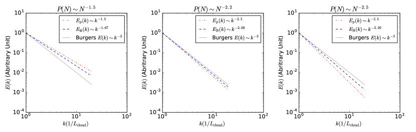
Figure 1: Comparison of the gravitational energy spectra and magnetic energy spectra for different cloud types. The red lines stand for the gravitational energy spectra and the blue lines stand for the magnetic energy spectra. The black lines stand for the kinetic energy spectra of the Burgers turbulence. The gravitational energy spectra are computed using Eq.4, where different surface density PDFs are assumed. The magnetic energy spectra are computed using Eq. 7, where, additionally, we assume a magnetic field-density relation $B\sim\rho^{1/2}$. The left panel shows a g-type cloud where the surface density PDF is $P(\Sigma)\sim\Sigma^{-1.5}$. The middle panel shows a cloud with $P(\Sigma)\sim\Sigma^{-2.2}$ where the turbulent, gravitational and magnetic energies are close to each other over multiple scales. The right panel shows a t-type cloud with a steep surface density PDF ($P(\Sigma)\sim\Sigma^{-3}$). Here we are only comparing the slopes, and the normalisation of the $y$-axis are not fixed.

$\gamma_{\Sigma}$	$\gamma_{B}$	$\epsilon_{\rm p}$	$\epsilon_{\rm B}$
Fiducial case, $B\sim\rho^{1/2}$
1.5	0.5	1.33	1.66
2	0.5	2	2
2.5	0.5	2.4	2.2
NGC6334
2.26	0.4	2.23	2.5
NGC6334 -corrected, Using Eq. 8
2.26	0.4	$2.39\pm 0.12$	$2.5\pm 0.08$

Table 2: A list of the slopes derived from observations. $\gamma_{\Sigma}$ is the slope of the surface density PDF, $\gamma_{B}$ is the slope of the magnetic field-density relation, $\epsilon_{\rm p}$ is the slope of the gravitational energy spectrum and $\epsilon_{\rm B}$ is the slope of the magnetic energy spectrum. The definitions of these quantities can be found in Table 1.

Assuming that beyond a critical density (typically $n_{\rm H_{2}}>300\;\rm cm^{-3}$, Crutcher et al. (2010)), the magnetic field-density relation $B\sim\rho^{1/2}$ holds universally for all molecular clouds, we discuss the effectiveness of magnetic support in these clouds. A typical molecular cloud should have a surface density PDF of $P(\Sigma)\sim\Sigma^{-2}$ (e.g. Lombardi et al., 2015), and this corresponds to a gravitational energy spectrum of $E_{\rm p}(k)\sim k^{-2}$ (Eq. 4). Assuming $B\sim\rho^{1/2}$, we can use Eq. 7 to derive the magnetic energy spectrum. In this fiducial case, the magnetic energy spectrum is $E_{\rm B}\sim k^{-2}$. Since both scales as $k^{-2}$, if the gravitational energy and the magnetic energy of a cloud are comparable on the cloud scale, we expect them to stay comparable as we move to smaller scales. This is the case where the gravitational energy and the magnetic energy reach a multi-scale energy equipartition. If turbulence in the molecular clouds is Burgers-like, we expect the turbulence energy to scale as $E_{\rm turb}\sim k^{-2}$, thus there should be a multi-scale energy equipartition between turbulence, gravity, and the magnetic field.

In Li & Burkert (2016), molecular clouds are classified into two categories. The regions whose surface density PDFs are shallower than $\Sigma^{-2}$ are called g-type clouds. In these regions, the gravitational energy spectra are shallow, and gravity dominates the cloud evolution on smaller scales. The regions whose surface density PDFs are steeper than $\Sigma^{-2}$ are called t-type clouds where turbulence can provide effective support against gravitational collapse. The new scaling relations from this paper allow us study the effect of magnetic field in these different cases. In Fig. 1, we plot the gravitational energy spectrum and magnetic spectrum for different cloud types. Assuming that the magnetic field-density relation $B\sim\rho^{1/2}$ holds universally, both the gravitational energy spectrum and the magnetic energy spectrum evolves with the cloud surface density PDF. Therefore, to understand the interplay between gravity and the magnetic field to a better accuracy, it is necessary to take the variations of the cloud surface density PDF into consideration.

One should also note that the more recently Bayesian analysis of Crutcher et al. (2010) suggest that at densities above $300\;\rm cm^{-3}$, $B\sim\rho^{0.65}$ is the preferred magnetic field-density relation. What differences does it make when one changes the slope of the magnetic field-density relation? Consider a typical molecular cloud whose surface density PDF is characterised by $P(\Sigma)\sim\Sigma^{-2}$, the gravitational energy spectrum is $E_{\rm p}(k)\sim k^{-2}$ (Eq. 4). Assuming $B\sim\rho^{0.65}$, the magnetic energy spectrum is $E_{\rm B}(k)\sim k^{-1.4}$ (Eq. 7). In most cases, the magnetic energy spectrum is much shallower than the gravitational energy spectrum, which indicates that magnetic fields would play a more important role as one moves to smaller scales. Since the clouds are already fragmented, we assume that on smaller ($\sim 0.1\;\rm pc$) scales, the densities of gravitational and magnetic energy are comparable, on larger scales, we expect the gravitational energy to exceed the magnetic energy by much. Therefore, a magnetic field-density relation $B\sim\rho^{0.65}$ would probably imply that magnetic field is dynamically unimportant on the large scale. This is similar to the conclusion by Crutcher et al. (2010). However, since the results of Crutcher et al. (2010) are obtained by collecting data from clouds with different structures, it is difficult to evaluate systematic effects. The current available measurements are consistent with magnetic fields staying in a multi-scale equipartition with the gravitational energy, but more future observations should be carried out in a systematic fashion to further constrain this.

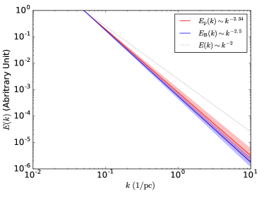
Figure 2: The gravitational and magnetic energy spectrum of the NGC6334 region. The red solid line stands for the gravitational energy spectrum of the region, the uncertainty of which is represented by the red shaded region. The blue solid line shows the magnetic energy spectrum of the region, and the uncertainty is represented by the blue shaded region. The kinetic energy spectrum of the Burgers turbulence ($E_{\rm k}\sim k^{-2}$) is plotted for reference. Here we are only comparing the slopes, and the normalisations of the $y$-axes are not fixed. See Sec. 3.2 for details.

3.2 Possible multi-scale energy equipartition in NGC6334

The NGC6334 star-forming region is perhaps the only region where magnetic field strength has been estimated over multiple scales (Li et al., 2015), and this allows us to study the multi-scale interplay between turbulence and gravity to a better detail. They found that $B\sim\rho^{0.4\pm 0.04}$. The relation holds from a few tens of a parsec down to $\sim 0.1\;\rm pc$. However, one should note that these are not direct measurements: the magnetic field strength is estimated using force balance, and can be biased. In spite of all these caveats, the measurements have produced the scaling relation we need to study the multi-scale interplay between turbulence and gravity.

Since we are aiming at an accurate comparison of the slopes of the gravitational and magnetic energy spectrum, it is beneficial to take the geometrical properties of the regions, e.g. how it fragments into account. The region is fragmented, and from their Fig. 3, we estimate $N\sim r^{-0.24}\sim k^{0.24}$ where $N$ is the number of regions . The surface density PDF of the region has been measured by Russeil et al. (2013) and Schneider et al. (2015) where $P(\Sigma)\sim\Sigma^{-2.26}$. The gravitational energy spectrum of the region can be computed with Eq. 4, which is $E_{\rm p}(k)\sim k^{-2.23}$. When the number of subregions of the cloud is taken into the analysis, using Eq. 8, $E_{\rm p,corr}(k)\sim k^{-2.39}$. For NGC6334, the measured magnetic field-density relation is $B\sim\rho^{0.4}$ (Li et al., 2015). Using Eq. 7, it gives a magnetic energy spectrum of $E_{\rm B}\sim k^{-2.5}$. The gravitational and magnetic energy spectrum are plotted in Fig. 2, and the scaling exponents are listed in Table 2. The slope of the magnetic energy spectrum resembles the that of gravitational energy spectrum, suggesting a multi-scale near equipartition between gravity and the magnetic field in NGC6334.

Although in NGC6334, the slopes still differ by $0.1$, this difference is not significant had one taken into account the uncertainties: the uncertainty of our formula for the slope of the gravitational energy spectrum is found to be around $5\%$ for the Orion complex (Li & Burkert, 2017). Since in this paper, we take the dependence of the number of regions on the scale into account explicitly, we expect a better accuracy. Taking the $5\%$ as an upper limit, the gravitational energy spectrum of the NGC6334 region should be $E_{\rm p}\sim k^{-2.39\pm 0.12}$. The slope of the magnetic field-density relation measured from Li et al. (2015) has an uncertainty of $0.04$. Assuming that this is the major contribution to the uncertainty of the magnetic energy spectrum, we have $E_{\rm B}\sim k^{-2.5\pm 0.08}$. After considering the uncertainties, the results are consistent with an exact multi-scale equipartition. between the gravitational and magnetic energy.

4 Conclusions

We present an analytical formalism to evaluate the distribution of magnetic energy over multiple scales in molecular clouds using the observed surface density PDF and the magnetic field-density relation.

In the fiducial case where a molecular cloud has a surface density PDF of $P(\Sigma)\sim\Sigma^{-2}$ and a magnetic field-density relation of $B\sim\rho^{1/2}$, the gravitational and magnetic energy reach a multi-scale near equipartition. For NGC6334 where estimates of magnetic field over multiple scales (10 pc to 0.1 pc) are available, our detailed analysis suggest that the energy equipartition between gravity and the magnetic field holds to a very good accuracy (where the slopes differ by $\sim 0.1$). Thus, if magnetic field is dynamically important on the cloud scale, we expect it to be important on much smaller scales, and would be able to influence the gravitational collapse over these scales.

Our analysis also reveal our lack of quantitative understanding of the role of magnetic fields in clouds: The slope of the magnetic field-density relation remains uncertain. Besides, according to our formalism, to properly evaluate the gravitational and magnetic energy densities as a function of the scale, one needs to measure both the surface density PDF and the magnetic field-density relation within different clouds. This should be achievable in the future.

It is seems likely that many more clouds would have energy equipartition similar to the NGC6334. However, if future observations indicate a steep slope in the magnetic field-density relation – a slope that is steeper than what is predicted by Eq. 10, it implies that there is an excess of magnetic energy density on smaller scales compared to the cloud scale, and presumably magnetic field is not important on the large scale, but becomes important as it gets amplified by some dynamo processes (e.g. Lazarian, 1993) during the collapse. On the other hand, if observations indicate a shallower slope, it would imply that the gas contained in small-scale structures has lost a significant fraction of the magnetic flux during the collapse, and in this case the magnetic field is probably regulating the collapse. The importance of the magnetic field might also be different in different clouds. Future observations should be able to to distinguish these possibilities.

Notes after the proof:
(1) Although the concept of magnetic energy spectrum is developed based on our earlier papers, a similar construction has been proposed by Han et al. (2004) (reviewed by Han (2017)), where, using pulsar rotation and dispersion measures, they found $E_{B}(k)\sim k^{-5/3}$. Their results are obtained using a different method, yet the values are consistent with ours.
(2) The equipartition of the spectral energy densities of the turbulence and gravity has been found in the simulation of Kritsuk et al. (2017).

References

- Alves et al. (2008) Alves F. O., Franco G. A. P., Girart J. M., 2008, A&A, 486, L13
- André et al. (2014) André P., Di Francesco J., Ward-Thompson D., Inutsuka S.-I., Pudritz R. E., Pineda J. E., 2014, Protostars and Planets VI, pp 27–51
- Bertoldi & McKee (1992) Bertoldi F., McKee C. F., 1992, ApJ, 395, 140
- Beuther et al. (2015) Beuther H., Ragan S. E., Johnston K., Henning T., Hacar A., Kainulainen J. T., 2015, A&A, 584, A67
- Crutcher (1999) Crutcher R. M., 1999, ApJ, 520, 706
- Crutcher et al. (2010) Crutcher R. M., Wandelt B., Heiles C., Falgarone E., Troland T. H., 2010, ApJ, 725, 466
- Federrath et al. (2010) Federrath C., Roman-Duval J., Klessen R. S., Schmidt W., Mac Low M.-M., 2010, A&A, 512, A81
- Fontani et al. (2016) Fontani F., et al., 2016, A&A, 593, L14
- Girichidis et al. (2014) Girichidis P., Konstandin L., Whitworth A. P., Klessen R. S., 2014, ApJ, 781, 91
- Han (2017) Han J. L., 2017, ARA&A, 55, 111
- Han et al. (2004) Han J. L., Ferriere K., Manchester R. N., 2004, ApJ, 610, 820
- Heyer & Brunt (2012) Heyer M. H., Brunt C. M., 2012, MNRAS, 420, 1562
- Hull et al. (2017) Hull C. L. H., et al., 2017, ApJ, 842, L9
- Kainulainen et al. (2009) Kainulainen J., Beuther H., Henning T., Plume R., 2009, A&A, 508, L35
- Kritsuk et al. (2007) Kritsuk A. G., Norman M. L., Padoan P., Wagner R., 2007, ApJ, 665, 416
- Kritsuk et al. (2017) Kritsuk A. G., Ustyugov S. D., Norman M. L., 2017, New Journal of Physics, 19, 065003
- Lazarian (1993) Lazarian A., 1993, in Krause F., Radler K. H., Rudiger G., eds, IAU Symposium Vol. 157, The Cosmic Dynamo. p. 429
- Li & Burkert (2016) Li G.-X., Burkert A., 2016, MNRAS, 461, 3027
- Li & Burkert (2017) Li G.-X., Burkert A., 2017, MNRAS, 464, 4096
- Li et al. (2011) Li H.-B., Blundell R., Hedden A., Kawamura J., Paine S., Tong E., 2011, MNRAS, 411, 2067
- Li et al. (2014) Li H.-B., Goodman A., Sridharan T. K., Houde M., Li Z.-Y., Novak G., Tang K. S., 2014, Protostars and Planets VI, pp 101–123
- Li et al. (2015) Li H.-B., et al., 2015, Nature, 520, 518
- Lombardi et al. (2015) Lombardi M., Alves J., Lada C. J., 2015, A&A, 576, L1
- Myers & Goodman (1988) Myers P. C., Goodman A. A., 1988, ApJ, 326, L27
- Panopoulou et al. (2016a) Panopoulou G. V., Psaradaki I., Tassis K., 2016a, MNRAS, 462, 1517
- Panopoulou et al. (2016b) Panopoulou G., et al., 2016b, MNRAS, 462, 2011
- Pillai et al. (2015) Pillai T., Kauffmann J., Tan J. C., Goldsmith P. F., Carey S. J., Menten K. M., 2015, ApJ, 799, 74
- Planck Collaboration et al. (2016) Planck Collaboration et al., 2016, A&A, 586, A136
- Russeil et al. (2013) Russeil D., et al., 2013, A&A, 554, A42
- Schneider et al. (2015) Schneider N., et al., 2015, MNRAS, 453, 41
- Soler et al. (2017) Soler J. D., et al., 2017, preprint, (arXiv:1702.03853)
- Tritsis et al. (2015) Tritsis A., Panopoulou G. V., Mouschovias T. C., Tassis K., Pavlidou V., 2015, MNRAS, 451, 4384
- Veltchev et al. (2016) Veltchev T. V., Donkov S., Klessen R. S., 2016, MNRAS, 459, 2432
- Zhang et al. (2014) Zhang Q., et al., 2014, ApJ, 792, 116