Accurate ray-tracing of realistic neutron star atmospheres
for constraining their parameters

Abstract

Thermal dominated X-ray spectra of neutron stars in quiescent transient X-ray binaries and neutron stars that undergo thermonuclear bursts are sensitive to mass and radius. The mass-radius relation of neutron stars depends on the equation of state that governs their interior. Constraining this relation accurately is thus of fundamental importance to understand the nature of dense matter. In this context we introduce a pipeline to calculate realistic model spectra of rotating neutron stars with hydrogen and helium atmospheres. An arbitrarily fast rotating neutron star with a given equation of state generates the spacetime in which the atmosphere emits radiation. We use the Lorene/nrotstar code to compute the spacetime numerically and the Atm24 code to solve the radiative transfer equations self-consistently. Emerging specific intensity spectra are then ray-traced through the neutron star’s spacetime from the atmosphere to a distant observer with the Gyoto code. Here, we present and test our fully relativistic numerical pipeline. To discuss and illustrate the importance of realistic atmosphere models we compare our model spectra to simpler models like the commonly used isotropic color-corrected blackbody emission. We highlight the importance of considering realistic model-atmosphere spectra together with relativistic ray tracing to obtain accurate predictions. We also insist on the crucial impact of the star’s rotation on the observables. Finally, we close a controversy that has been appearing in the literature in the recent years regarding the validity of the Atm24 code.

1 Introduction

Neutron stars create extreme environments that harbor forms of ultra-dense matter that cannot be reproduced on Earth. The very complex properties of the stellar matter are encapsulated in the equation of state (EoS) that allows to close the system of equations describing the star’s equilibrium. This EoS is the link between the nuclear physics in the interior of the neutron star and astrophysical observables. In particular, a specific EoS will only allow certain pairs of values of neutron star mass $M$ and radius $R$ (see e.g. Haensel et al., 2007). Constraining the pair $(M,R)$ for a particular neutron star thus gives access to the nature of the EoS (for a recent review see Özel & Freire, 2016). We note that the star’s rotation has an impact on the $M$-$R$ relation and that the relation that is generally represented in typical figures is obtained for non-rotating stars.

Neutron star masses and radii may be constrained by various methods, such as

• the modeling of pulse profiles for sources that show an oscillating light curve most probably due to a rotating hot spot on the neutron star’s surface;

• the analysis of kHz quasi-periodic oscillations seen in the neutron star’s power density spectrum;

• the spectroscopic study of neutron stars in low-mass X-ray binaries (LMXB) that show so-called type-I X-ray bursts, i.e. a sudden burning of the fuel accreted from the secondary star;

• the modeling of thermal spectra from cooling isolated neutron stars or thermal dominated spectra of neutron stars in quiescent LMXB (qLMXB).

For reviews of these methods and of their limitations see e.g. Miller (2013); Miller & Lamb (2016); Özel & Freire (2016); Haensel et al. (2016). In this article we focus on the spectral methods, and more specifically on type-I bursters. This choice is in particular motivated by the fact that LMXB tend to have magnetic fields of the order of $10^{8-9}$ G, which is weak for a neutron star. It is thus fair to assume that the magnetic field does not influence the radiative properties of the atmosphere (Miller, 2013), which greatly simplifies the problem. We note that the numerical methods we present here are as well adapted for qLMXB, and could be easily developed in future works to model pulse profiles (in a scarcely magnetized environment).

Type-I bursters, in particular when they show photospheric radius expansion (PRE, see e.g. Fujimoto & Taam, 1986; van Paradijs & Lewin, 1987), have been used to constrain masses and radii of neutron stars ever since the method was proposed by van Paradijs (1979). The interpretation of observational data in the framework of this method may suffer from a series of limitations that can be divided into two main issues:

• the correct modeling of the emitted spectra;

• the way the effects of strong gravity are taken into account.

We will now review the recent progress in these two directions.

Regarding the modeling of the emitted spectra, it is first possible that not all the emission comes from the surface of the star (but for instance from residual accretion), and that not the whole surface of the star is emitting radiation (Miller & Lamb, 2016). We will assume in the remaining of the article that the full surface of the star, and it only, emits radiation. The main source of difficulty is then to model the emission arising from the star’s atmosphere.

The best constraints obtained from spectral methods use data recorded by the Rossi X-ray Timing Explorer (RXTE), using color-corrected blackbody emission at the surface of the star (Özel et al., 2009, 2016). Having a huge effective area, RXTE was able to collect a sufficient number of counts within milliseconds, allowing to make proper spectral analysis. Nevertheless, using a color-correction factor is always a simplified treatment which boils down to only shifting the blackbody radiation to mimic the emission from a true atmosphere. In the recent years, realistic atmosphere models have been developed to study neutron stars in type-I bursters and estimate their masses and radii.

There exist two classes of neutron star atmosphere models in the literature. The first class are model atmospheres which are approximate for the reason that they oversimplify the process of electron scattering (Heinke et al., 2006; Webb & Barret, 2007; Guillot et al., 2011). This class of neutron star model atmospheres is available in the widely used xspec (Arnaud, 1996) software fitting package. The second class of available model atmospheres does include accurate Compton scattering process, which is critically important to model atmospheres of hot neutron stars (with effective temperature of a few times $10^{7}$ K, characteristic of X-ray bursters) and their spectra (Madej, 1989, 1991a, 1991b; Madej et al., 2004; Majczyna et al., 2005; Suleimanov et al., 2011, 2012, 2016). Those models were successfully used for the mass and radius determination of non-rotating NS (Majczyna & Madej, 2005; Kuśmierek et al., 2011; Suleimanov et al., 2016, and references therein). We would like to point out here that only model atmospheres with Compton scattering fully taken into account can be used for mass and radius determination. Recently we proved that the Compton redistribution functions that we use in the radiative transfer equations are computed with excellent precision (Madej et al., 2017).

Regarding the impact of strong gravity, studies have been devoted to its effect on the radiative transfer in the atmosphere itself, as well as on the subsequent propagation of photons towards the distant observer. Most spectroscopic studies that aim at constraining neutron stars’ properties from thermal X-ray spectra of type-I bursters approximate the effects of general relativity by a single scalar factor, the surface gravitational redshift $z$. Such a scalar correction is sufficient to represent relativistic effects provided the thickness of the neutron star’s atmosphere is small compared to the radius of the star. Only recently, Medin et al. (2016) presented models of geometrically thick neutron-star atmospheres with accurate Compton scattering, taking into account the relativistic bending in the radiative transfer process itself, within the neutron star’s atmosphere.

The effects of strong gravity on the subsequent propagation of photons from the atmosphere to the distant observer has been the subject of a series of studies in the past decade. Cadeau et al. (2005, 2007) compared ray-tracing of photons in an approximate analytical spacetime with no shape modification of the star to ray-tracing of photons in an exact numerical neutron star spacetime (Stergioulas & Friedman, 1995) with the deformation of the surface taken into account. These studies lead to the conclusion that the oblate shape of the rotating star is the most important factor that should be considered. A recent series of papers by Bauböck et al. (2012, 2013, 2015) studied the importance of the rotation of the star as well as the quadrupole moment of the metric considering an analytical approximation to the exact neutron star metric, namely the Hartle & Thorne (1968) metric. The validity of this analytical approximation has been studied by Berti et al. (2005); Bauböck et al. (2013) and showed a satisfactory agreement for most astrophysical contexts.

An interesting very recent series of papers by Nättilä & Pihajoki (2017); Nättilä et al. (2017) is investigating in the same direction as our paper. It describes a new open-source ray-tracing code for neutron-star observables computation in approximate spacetimes, and presents the first direct fit to bursting neutron star data of model atmospheres (as contrasted to all previous fits performed with modified blackbodies). It is obviously of crucial importance that more than one numerical pipeline like ours should be published so that cross-checks of the rather involved outputs can be made.

Recent confirmation of the origin of short gamma-ray bursts as mergers of binary neutron-star systems (Abbott et al., 2017a, b, c) creates a new method of establishing neutron stars’ parameters. From the observations of tidal deformation imprinted on the waveform’s phase during the last orbits of the inspiral, one can distill the information on the size of the star and the stiffness of the EoS. The analysis performed in Abbott et al. (2017a) suggests that the component stars taking part in the merger had radii most likely smaller than 14 km at the measured mass range around $1.4\ M_{\odot}$.

The aim of this article is to present a numerical pipeline that implements the most accurate simulated neutron star spectrum to date, taking into account at the same time a precise atmospheric model, and considering all general-relativistic effects of the star’s geometry on the photon propagation. We compute an accurate numerical metric that in particular takes into account the exact deformation of the star due to its rotation. We solve the hydrostatic and radiative transfer problem in the neutron star’s atmosphere incorporating the exact value of the local (varying) surface gravity at the star’s surface. This local spectrum is then transported to a distant observer by means of a ray-tracing code that adheres to the exact numerical metric of the neutron star. An obvious interest of such a numerical pipeline is to provide a practical testbed for approximate methods, that are faster and more adapted for fitting data. However, our model can also be used to produce tables of model spectra that could be implemented in xspec and used for fitting data. Indeed, we will see below that the computing time necessary to produce a spectrum is reasonable for this prospect ($\approx 5$ min on a $2.9$ GHz Intel Core i7 processor of a personal laptop to produce one spectrum). Moreover, such a pipeline also offers the possibility to investigate in full details the impact of the EoS on the resulting spectrum, as well as to accurately predict the observables associated to ”extreme” systems that have not yet been observed to date: very fast-rotating and very massive neutron stars. We highlight that our pipeline is for the time being only partially open-source, but we aim at making it fully open-source in the close future.

The numerical method is presented in Section 2, and the results of the simulations in Section 3. Section 4 summarizes our work and gives future directions. Appendix A demonstrates the validity of the Atm24 code, that has been questioned in recent articles.

2 Description of the methods

Images and spectra of neutron stars are computed following the sketch of Figure 1.

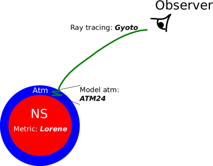
Figure 1: Sketch of the methods used to compute images and spectra of neutron stars. The neutron star is depicted in red, its structure and spacetime metric is computed with the Lorene/nrotstar code. Its atmosphere is represented in blue (not to scale, the atmosphere is extremely thin as compared to the star’s radius, typically $10$s of cm compared to $10$ km). The radiative transfer equation is solved there together with hydrostatic equilibrium with the Atm24 code. Finally, the emitted photons are ray-traced to a distant observer using the Gyoto code which incorporates the neutron star’s metric computed by Lorene/nrotstar.

This Section describes the various pieces that appear in that sketch.

2.1 Spacetime metric

To describe the spacetime generated by the neutron star we adopt the quasi-isotropic coordinates $(t,r,\theta,\varphi)$. For simplicity we assume stationarity and axisymmetry, with Killing vectors $\boldsymbol{\partial}_{t}$ and $\boldsymbol{\partial}_{\varphi}$ corresponding to time and rotational symmetries. Under the assumption of pure rotational fluid motion about the symmetry axis, the general metric element reads

$$\mathrm{d}s^{2}=g_{\mu\nu}\,\mathrm{d}x^{\mu}\mathrm{d}x^{\nu} = -N^{2}\mathrm{d}t^{2}+A^{2}\left(\mathrm{d}r^{2}+r^{2}\mathrm{d}\theta^{2}\right)$$ (1)

$$+B^{2}r^{2}\sin^{2}\theta\left(\mathrm{d}\varphi-\omega\mathrm{d}t\right)^{2},$$

where $N$, $A$, $B$ and $\omega$ are four functions of $(r,\theta)$, $N$ being called the lapse function. The fluid 4-velocity $\mathbf{u}$ is a linear combination of the two Killing vectors (pure rotational motion hypothesis): $\mathbf{u}=u^{t}\left(\boldsymbol{\partial}_{t}+\Omega\,\boldsymbol{\partial}_{\varphi}\right)$, where the contravariant time component of the 4-velocity $u^{t}$ is expressible as $u^{t}=\Gamma/N$, with $\Gamma$ the Lorentz factor of the fluid with respect to the zero angular momentum observers (ZAMO). In the following we will assume rigid rotation, i.e. a constant value of the star’s angular velocity $\Omega=u^{\phi}/u^{t}=\mathrm{d}\phi/\mathrm{d}t$.

The metric of a neutron star rigidly rotating with angular frequency $\Omega$ is fully fixed once the dense matter equation of state inside the star is selected and the central density $\rho_{c}$ (or pressure $P_{c}$) is chosen. This is a natural choice for computational purposes which allows to integrate the general relativistic equations of structure for a uniformly rotating body. Two out of the three following global quantities, which are well defined in general relativity for a rotating star, also uniquely determine a rotating configuration and the properties of the metric at the star’s surface:

• the gravitational (ADM, Arnowitt et al. 1961) mass $M$,

• the baryon mass $M_{b}$,

• the total angular momentum $J$.

For the relations between these global parameters, properly defining sequences of stellar configurations, see e.g. Zdunik et al. (2006). Another important quantity is the circumferential stellar radius $R$, defined such that the circumference of the star in the equatorial plane, as given by the metric tensor, is $2\pi\,R$. Then $R$ is related to the equatorial quasi-isotropic coordinate radius $r_{\mathrm{eq}}$ by the metric function $B(r,\theta)$, according to $R=B(r_{\mathrm{eq}},\pi/2)\,r_{\mathrm{eq}}$.

In order to obtain the accurate solutions for rotating neutron stars configurations at arbitrarily high spin (i.e., beyond the slow-rotation approximation), we employ the nrotstar code (Gourgoulhon, 2010) built using the free and open-source Lorene library (Gourgoulhon et al., 2016, http://www.lorene.obspm.fr), which provides spectral-methods solvers to the Einstein equations. The nrotstar code allows for fast computation of the stellar surface, described by the coordinate radius $r_{\mathrm{surf}}(\theta)$ as a function of $\theta$, the 4-velocity of the fluid at the surface, as well as the fluid 4-acceleration at the surface. In all the star, the fluid 4-acceleration $\mathbf{a}$ has covariant components given by

$$a_{\mu}=u^{\nu}\nabla_{\nu}u_{\mu}=-\partial_{\mu}\left(\mathrm{ln}\,u^{t}\right).$$ (2)

The second expression results from the assumptions of circularity and rigid rotation, i.e. from the fact that the fluid 4-velocity is $\mathbf{u}=u^{t}\mathbf{k}$, where $\mathbf{k}=\boldsymbol{\partial}_{t}+\Omega\boldsymbol{\partial}_{\varphi}$ is a Killing vector, since $\Omega$ is constant. The surface gravity $g_{\rm s}$ is the norm of $\mathbf{a}$ at the stellar surface:

$$g_{\rm s}=\sqrt{a_{\mu}a^{\mu}}=A\sqrt{\left(a^{r}\right)^{2}+r^{2}\left(a^{\theta}\right)^{2}},$$ (3)

where the second equality results from the metric (1) and the fact that Eq. (2) along with the hypothesis of stationarity and axisymmetry imply $a_{t}=a_{\varphi}=0$.

The first integral of the relativistic Euler equation governing the fluid motion is $h/u^{t}=\mathrm{const}$ (see e.g. Gourgoulhon, 2010), where $h$ is the fluid’s relativistic specific enthalpy. At the surface of the star, the fluid’s internal energy and pressure tend to zero, so that $h=1$. It follows from the first integral that the stellar surface is an isosurface of $u^{t}$. From Eq. (2), we conclude that the fluid 4-acceleration gives the normal to the stellar surface (which is a timelike hypersurface in spacetime). For some photon escaping the star with a tangent null 4-vector $\mathbf{p}$, the emission angle $\epsilon$ between the direction of photon emission in the frame corotating with the star and the local normal reads

$$\cos\epsilon=-\frac{\mathbf{n}\cdot\mathbf{p}}{\mathbf{u}\cdot\mathbf{p}}$$ (4)

where $\mathbf{n}=\mathbf{a}/g_{\rm s}$ is the unit spacetime normal to the stellar surface, $\mathbf{u}$ is the surface value of the fluid’s 4-velocity and a dot denotes the scalar product taken with the metric (1). As we will see below, all these quantities are necessary for the ray-tracing and the atmosphere radiative transfer calculations.

2.2 Directional atmospheres

We compute local spectra emitted in the star’s hydrogen/helium atmosphere via the radiative transfer code Atm24 (Madej et al. 2018, in preparation). Previous versions of the code were described in Madej et al. (2004); Majczyna et al. (2005). We note that the neutron star’s atmosphere has a very small height ($\approx 1$ m as compared to the star’s radius of $\approx 10$ km) so that the radiative transfer computation is essentially local. This allows us to neglect relativistic effects in this Section and use a Newtonian treatment.

The equation of radiative transfer in a plane-parallel atmosphere can be written in the following form:

$$\mu {\partial I_{\nu}(z,\mu)\over{\rho\partial z}}=\kappa^{\prime}_{\nu}(1-e^{-h\nu/kT})(B_{\nu}-I_{\nu})$$

$$+ \left(1+{c^{2}\over{2h\nu^{3}}}I_{\nu}\right)\oint\limits_{\omega^{\prime}}{d\omega^{\prime}\over 4\pi}\int\limits_{0}^{\infty}{\nu\over{\nu^{\prime}}}\sigma(\nu^{\prime}\rightarrow\nu,\vec{n}{{}^{\prime}}\cdot\vec{n})I_{\nu^{\prime}}(z,\vec{n}^{\prime})d\nu^{\prime}$$

$$- \,I_{\nu}(z,\mu)\oint\limits_{\omega^{\prime}}{d\omega^{\prime}\over{4\pi}}\int\limits_{0}^{\infty}\sigma(\nu\rightarrow\nu^{\prime},\vec{n}\cdot\vec{n}{{}^{\prime}})(1+{c^{2}\over{2h{\nu^{\prime}}^{3}}}I_{\nu^{\prime}})\,d\nu^{\prime}\,.$$

assuming that sources of true absorption ($\kappa_{\nu}$) and thermal emission ($j_{\nu}=\kappa_{\nu}B_{\nu}$) are in local thermodynamic equilibrium (LTE). Here, $z$ is the geometrical depth, and $\mu=\cos\epsilon$. Eq. (2.2) does not include relativistic corrections on the neutron star surface, which will be treated in the next Section. The above equation of transfer was a starting point in earlier investigations (Sampson, 1959; Madej, 1989, 1991a, 1991b).

Variable $\sigma_{\nu}$ denotes the coefficient of Compton scattering at a given frequency $\nu$ integrated over all incoming frequencies $\nu^{\prime}$. The variable $\sigma(\nu\rightarrow\nu^{\prime},\vec{n}\cdot\vec{n}{{}^{\prime}}$) denotes the differential Compton scattering cross section, and $\kappa_{\nu}^{\prime}$ is the absorption coefficient uncorrected for stimulated emission. All the opacity coefficients are given for 1 gram of matter (units of cm² g^-1). The relation between the differential Compton scattering cross section and the integrated Compton scattering coefficient is given by the following equation:

$$\sigma_{\nu}=\oint\limits_{\omega^{\prime}}{d\omega^{\prime}\over{4\pi}}\int\limits_{0}^{\infty}\sigma(\nu\rightarrow\nu^{\prime},\vec{n}\cdot\vec{n}{{}^{\prime}})d\nu^{\prime}.$$ (6)

Compton scattering differential cross section must fulfil the relation:

$$\sigma(\nu\rightarrow\nu{{}^{\prime}},\vec{n}\cdot\vec{n}{{}^{\prime}})\,\nu^{2}e^{-h\nu/kT}=\,\sigma(\nu{{}^{\prime}}\rightarrow\nu,\vec{n}{{}^{\prime}}\cdot\vec{n})\,{\nu^{\prime}}^{2}e^{-h\nu^{\prime}/kT}\>,$$ (7)

which results from the detailed balance of this process in global thermodynamic equilibrium (Pomraning, 1973).

Moreover, we define new variables:

$$\kappa_{\nu}=\kappa_{\nu}{{}^{\prime}}\,(1-e^{-h\nu/kT})$$ (8)

and

$$\sigma(\nu\rightarrow\nu^{\prime},\vec{n}\cdot\vec{n}^{\prime})\,=\sigma_{\nu}\,\phi(\nu,\nu^{\prime},\vec{n}\cdot\vec{n}^{\prime})\>,$$ (9)

where the Compton scattering redistribution function $\phi$ is normalized to unity:

$$\oint\limits_{\omega^{\prime}}{{d{\omega^{\prime}}}\over 4\pi}\int\limits_{0}^{\infty}\phi(\nu,\nu^{\prime},\vec{n}\cdot\vec{n}^{\prime})\,d{\nu^{\prime}}=1\,.$$ (10)

Angle-dependent Compton scattering redistribution function $\phi$ was approximated by its zeroth angular moment,

$$\Phi(\nu,\nu^{\prime})=\oint\limits_{\omega^{\prime}}\phi(\nu,\nu^{\prime},\vec{n}\cdot\vec{n}{{}^{\prime}})\,{d{\omega^{\prime}}\over 4\pi}\,.$$ (11)

Then, we write the equation of transfer (2.2) on the monochromatic optical depth scale $d\tau_{\nu}=-(\kappa_{\nu}+\sigma_{\nu})\rho dz$:

$$\mu\,{\partial I_{\nu}\over{\partial\tau_{\nu}}} = I_{\nu}-\epsilon_{\nu}\,B_{\nu}\>-(1-\epsilon_{\nu})J_{\nu}$$

$$+ (1-\epsilon_{\nu})J_{\nu}\,\int\limits_{0}^{\infty}\Phi(\nu,\nu^{\prime})\,(1+{c^{2}\over{2h{\nu^{\prime}}^{3}}}J_{\nu^{\prime}})\,d\nu^{\prime}\>$$

$$- (1-\epsilon_{\nu})\,(1+{c^{2}\over{2h\nu^{3}}}J_{\nu})\,\int\limits_{0}^{\infty}\Phi(\nu,\nu^{\prime})J_{\nu^{\prime}}$$

$$\times \,{\left({\nu\over{\nu^{\prime}}}\right)}^{3}\exp\left[-{{h(\nu-{\nu^{\prime}})}\over{kT}}\right]\,d\nu^{\prime}.$$

Dimensionless monochromatic absorption is defined as $\epsilon_{\nu}=\kappa_{\nu}/(\kappa_{\nu}+\sigma_{\nu})$. We point out here that the equation of transfer, Eq. (2.2), is not linear and is quadratic with respect to the unknown $J_{\nu}$.

Here we stress that the equation of transfer assumes that Compton scattering is an isotropic process. The angle-integrated normalized redistribution function $\Phi(\nu,\nu^{\prime})$ was derived from the exact redistribution function $R_{1}$ as presented in Madej et al. (2017).

The above equation of transfer is accompanied by two boundary conditions, the first being:

$${d\over{d\tau_{\nu}}}\,(f_{\nu}J_{\nu})\,=H_{\nu}(0)$$ (13)

at the top of the model atmosphere ($\tau_{\nu}=0$). At the bottom we require $J_{\nu}=B_{\nu}$, according to the usual thermalization condition. The variable $f_{\nu}$ denotes the well-known Eddington factor.

In this paper we solve the above equation precisely iterating Eddington factors $f_{\nu}$ at all frequencies and optical depth points. In such a way, we exactly reproduce the angular behavior of the radiation field, and determine the angular stratification of the specific intensity $I_{\nu}(\tau,\mu)$.

Our equations and the Compton redistribution functions (Nagirner & Poutanen, 1993; Suleimanov et al., 2012) work correctly for both large and small energy exchange between X-ray photons and free electrons at the time of scattering. The resulting model atmosphere and theoretical spectra represent the most accurate quantum mechanical solution of the Compton scattering problem, as shown in our recent paper Madej et al. (2017). The above equations produce accurate solutions also when the initial photon energy before or after scattering exceeds the electron rest mass ($m_{e}c^{2}=511$ keV).

In our numerical procedure, the equation above is solved with the structure of the gas kept in radiative, hydrostatic, and ionization equilibrium simultaneously. Condition of radiative equilibrium implies on each depth level $\tau_{\nu}$ that

$$\int\limits_{0}^{\infty}H_{\nu}(\tau_{\nu})\,d\nu={\sigma_{R}T_{\rm eff}^{4}\over{4\pi}}\,,$$ (14)

where $\sigma_{R}=5.66961\times 10^{-5}$ (in cgs units). The second condition of hydrostatic equilibrium can be expressed in the usual form

$${dP_{g}\over{d\tau}} = {g_{\rm s}\over{(\kappa+\sigma)_{std}}}-{dP_{r}\over{d\tau}}$$

$$= {g_{\rm s}\over{(\kappa+\sigma)_{std}}}-{4\pi\over c}\,\int\limits_{0}^{\infty}{\kappa_{\nu}+\sigma_{\nu}\over{(\kappa_{\nu}+\sigma_{\nu})_{std}}}\,H_{\nu}\,d\nu\,$$

where $g_{\rm s}$ is the surface gravity, which is computed self-consistently along the neutron star’s surface with Lorene/nrotstar. The standard opacities and standard optical depth $\tau$ correspond to the same variables at the arbitrarily fixed frequency. The hydrostatic equation is coupled to the radiative transfer by the mass density $\rho$ that appears in the optical depth $\tau_{\nu}$. We use the equation of state of an ideal gas and compute ionization and excitation populations, therefore absorption coefficient $\kappa_{\nu}$, using Saha and Boltzmann equations (assuming local thermodynamic equilibrium).

The inputs of Atm24 thus are:

• the composition of the atmosphere, which is assumed here to be composed of hydrogen and helium, in solar abundance,

• the surface effective temperature, assumed here to be $T_{\mathrm{eff}}=10^{7}$ K,

• the surface gravity $g_{\rm s}$, self-consistently computed by Lorene/nrotstar along the surface.

The output is the local spectrum of emitted specific intensity $I_{\nu}(\nu,\mu)$, as a function of emitted frequency and cosine of emission angle. This output can also slightly depend on the polar angle $\theta$ connected to the star’s shape, given that the surface gravity becomes a function of $\theta$ for rotating stars, which we fully take into account in this paper computing the accurate distribution of $I_{\nu}(\nu,\mu,\theta)$.

We note that the validity of the Atm24 code has been recently put in question by Suleimanov et al. (2012), as well as more recently by Medin et al. (2016), on the basis that one model spectrum obtained by these authors differs from that computed by Atm24. We show in Appendix A that the Atm24 spectrum used for comparison simply was not properly converged, as was suggested in the discussion of Suleimanov et al. (2012). Appendix A shows that fully converged Atm24 spectra essentially do agree with Suleimanov et al. (2012).

2.3 Ray tracing

The open-source ray tracing code Gyoto (see Vincent et al., 2011, 2012, and http://gyoto.obspm.fr) is used to compute null geodesics backwards in time, from a distant observer towards the neutron star. Photons are traced in the neutron star’s metric as computed by the Lorene/nrotstar code. Once the neutron star’s surface is reached, the emission angle $\epsilon$ between the photon’s direction of emission and the local normal is evaluated following Eq. (4). Given the observed photon frequency $\nu_{\mathrm{obs}}$, the emitted frequency $\nu_{\mathrm{em}}$ is found knowing the redshift which is defined by the local value of the 4-velocity at the neutron star’s surface and which is computed by Lorene/nrotstar. Finally, the local surface gravity is also known from the Lorene output. Consequently, the local value of the emitted specific intensity $I_{\nu}^{\mathrm{em}}(\nu_{\mathrm{em}},\mu,g_{\rm s}(\theta_{\mathrm{em}}))$ at a polar angle $\theta_{\mathrm{em}}$, can be interpolated from the output table computed by the Atm24 code. The observed specific intensity is then $I_{\nu}^{\mathrm{obs}}=\nu_{\mathrm{obs}}^{3}/\nu_{\mathrm{em}}^{3}\,I_{\nu}^{\mathrm{em}}$. The map of observed specific intensity (i.e. the image) in the frame of a distant observer is thus at hand. Performing such computations for a set of observed photon frequencies and summing these images over the observer’s screen pixels (i.e. over the directions of photon reception) allows to obtain an observed spectrum $F_{\nu}^{\mathrm{obs}}$.

3 Stellar and atmospheric models, ray-traced images and spectra

3.1 Stellar models

We consider two models of neutron stars described by the SLy4 dense-matter equation of state (Chabanat et al., 1998; Douchin & Haensel, 2001), supplemented with the description of the neutron star’s crust of Haensel & Pichon (1994): a non-rotating configuration and a configuration rotating rigidly at 716 Hz (matching the frequency of currently fastest-spinning pulsar PSR J1748-2446ad, Hessels et al. 2006). For both configurations we select a gravitational mass of $M=1.4\ M_{\odot}$. In general, the surface gravity of a non-rotating neutron star is

$$g_{{\rm s},0\,{\rm Hz}}=\frac{GM}{R^{2}}\frac{1}{\sqrt{1-2GM/Rc^{2}}}.$$ (16)

For a mass of $M=1.4\ M_{\odot}$ and considering the SLy4 EoS, $g_{{\rm s},0\,{\rm Hz}}=1.68\times 10^{14}\,\mathrm{cm}\,\mathrm{s}^{-2}$ (see Bejger & Haensel 2004 for a summary for other EoS models). In contrast, a rotating neutron star has a surface gravity varying along the $\theta$ direction, as described in Sect. 2.1. In Fig. 2 we compare the surface gravities for both our models. The resulting values of surface gravities and circumferential radii are of order $g_{\rm s}=1.5\times 10^{14}\,\mathrm{cm}\,\mathrm{s}^{-2}$ and $R=12$ km. In comparison, the neutron star model often considered as a reference, with $M=1.4\ M_{\odot}$ and R = 10 km, yields $g_{\rm s}=2.43\times 10^{14}\,\mathrm{cm}\,\mathrm{s}^{-2}$ (Bejger & Haensel, 2004).

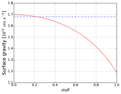
Figure 2: Comparison of surface gravities between a non-rotating neutron star (blue dash-dotted line at a constant value of $1.68\times 10^{14}\,\mathrm{cm}\,\mathrm{s}^{-2}$) and for a neutron star rigidly rotating at 716 Hz (red line, with values between $1.7\times 10^{14}\,\mathrm{cm}\,\mathrm{s}^{-2}$ for the pole at $\sin\theta=0$ and $1.19\times 10^{14}\,\mathrm{cm}\,\mathrm{s}^{-2}$ for the equator at $\sin\theta=1$). In both cases the gravitational mass equals $1.4\ M_{\odot}$.

We also compare the surface figures of stars. Figure 3 shows them in coordinate values for both selected configurations and compare them with the slow-rotation approximation to the shape of the surface:

$$r\left(\theta\right)=r_{\mathrm{eq}}-\left(r_{\mathrm{eq}}-r_{p}\right)\cos^{2}\theta,$$ (17)

where $r_{\mathrm{eq}}$ and $r_{p}$ are the equatorial and polar quasi-isotropic radii. This equation is used for instance in the Hartle-Thorne metric used by Bauböck et al. (2012). Assuming that the polar and equatorial radii are known, the error introduced by using the slow-rotation approximation at the rotational frequency of 716 Hz and mass $1.4\ M_{\odot}$ for the SLy4 EoS is maximally about 100 m in radius (for comparison, the maximal difference at 900 Hz is about 0.5 km).

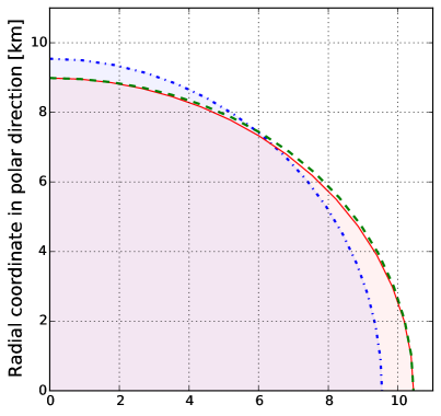
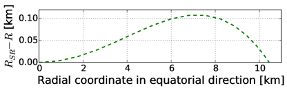
Figure 3: Surface figures for selected configurations in coordinate values. The blue dash-dotted line denotes the non-rotating star (circumferential radius $R_{0\,\mathrm{Hz}}=11.72$ km). The red line denotes the surface of the star rotating at 716 Hz (equatorial circumferential radius $R_{716\,\mathrm{Hz}}=12.65$ km, $r_{p}/r_{\mathrm{eq}}=0.86$). The green dashed line is the slow-rotation approximation of Eq. (17). The lower panel presents the difference between the shape of the rotating star obtained with Lorene/nrotstar, and the slow-rotation approximation of Eq. (17).

The spacetime generated by a rotating star in full general relativity is different from the slow-rotation approximation. Figure 4 shows the comparison of the metric function lapse $N$ with its approximation $1-M/r$, and the frame-dragging metric term (shift vector component $\omega=-\beta^{\phi}$) with $2J/r^{3}$, where $J$ is the total angular momentum of the configuration rotating at 716 Hz (see also Gourgoulhon 2010).

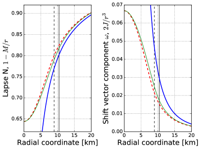
Figure 4: Left panel: Lapse function $N$ in polar (red dashed line) and equatorial (solid green line) direction compared with its slow-rotation approximation $1-M/r$ (solid blue). Right panel: Frame-dragging metric term (shift vector component $\omega=-\beta^{\phi}$) in polar (red dashed line) and equatorial (solid green line) direction compared with the slow-rotation approximation $2J/r^{3}$ (solid blue), $J$ denoting the total angular momentum of the star. Vertical lines denote the surface of the star: dashed for polar direction, solid for equatorial direction.

3.2 Local spectra

The local spectra are computed by Atm24 for an atmosphere made of hydrogen and helium in solar abundance and an effective temperature of $T_{\mathrm{eff}}=10^{7}$ K. All models used in this paper were computed with a large number of iterations, and they achieved satisfactory convergence after 500-600 iterations depending on the value of surface gravity (see Appendix A for explanation). They are shown in Fig. 5. The full range of surface gravities spanned by the non-rotating and rotating configurations has for bounds $1.19\times 10^{14}$ and $1.70\times 10^{14}$, in cgs units. This variation of $\approx 40\%$ of the surface gravity leads to a tiny variation of a fraction of a percent in the resulting local spectrum, which is thus scarcely sensitive to the local surface gravity. Consequently, Fig. 5 shows the Atm24 spectrum at one unique value of surface gravity, equal to $g_{\rm s}=1.7\times 10^{14}\,\mathrm{cm}\,\mathrm{s}^{-2}$. Fig. 5 also shows a color-corrected blackbody spectrum as defined by

$$I_{\nu}^{\mathrm{BB\,corr}}=\frac{1}{f_{\mathrm{cor}}^{4}}B_{\nu}(T=f_{\mathrm{cor}}T_{\mathrm{eff}})$$ (18)

where $B_{\nu}$ is the Planck function and $f_{\mathrm{cor}}=1.4$ is the color-correction factor.

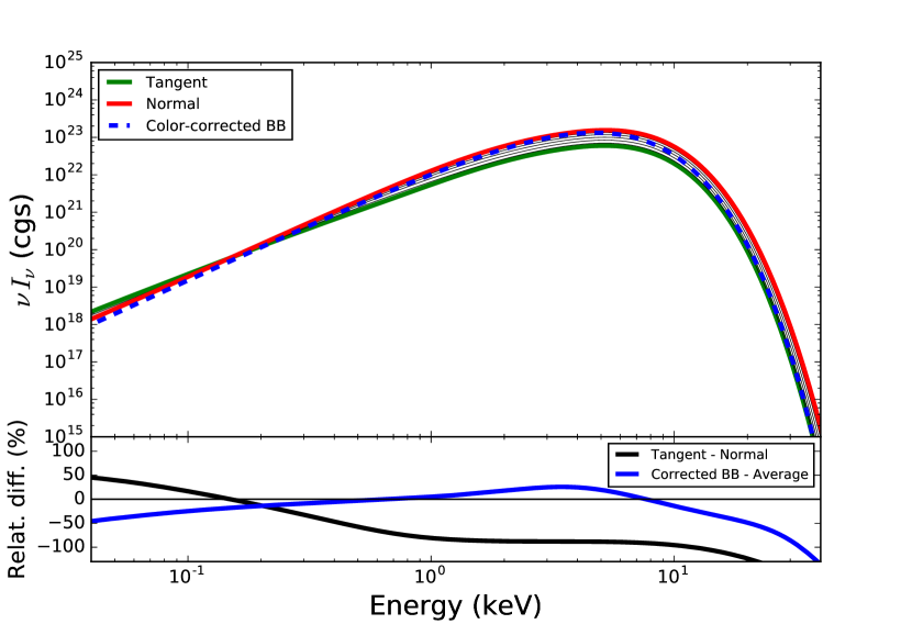
Figure 5: Local spectra emitted at the star’s surface. Top panel: the thick dashed blue curve shows a color-corrected blackbody at $T_{\mathrm{eff}}=10^{7}$ K which is also the effective temperature of the neutron star’s surface used in Atm24. The color-correction factor is $f_{\mathrm{cor}}=1.4$. All other curves are obtained by Atm24 after solving the radiative transfer equation in the neutron star’s atmosphere. The surface gravity equals $1.7\times 10^{14}\,\mathrm{cm}\,\mathrm{s}^{-2}$ (but the effect of this parameter is very small). Each solid thin black curve corresponds to a different emission angle $\epsilon$, with the thick red curve corresponding to emission along the local normal and the thick green curve to emission tangent to the star’s surface. Bottom panel: the percentage difference (defined as $(X_{a}-X_{b})/(X_{a}+X_{b})\times 200$) between these two extreme angles in black (tangent minus normal), and the percentage difference between the corrected blackbody and the Atm24 spectrum averaged over emission angle in blue.

Fig. 5 also represents in its lower panel comparisons between various spectra. It first compares the corrected blackbody spectrum to the Atm24 spectrum averaged over the cosine of the emission angle $\mu=\cos\epsilon$. The angle-averaged specific intensity, at frequency $\nu$ and latitude $\theta$, is equal to twice the usual mean intensity:

$$I_{\nu}^{\mathrm{angle-averaged}}(\nu,\theta)=2J_{\nu}(0)=\int_{\mu}I_{\nu}(\nu,\mu,\theta)\,\mathrm{d}\mu.$$ (19)

The averaged Atm24 spectrum is overall close to the corrected blackbody, but a closer look reveals significant intensity differences at the level of $\approx 50\%$ for both the low and high energy spectral wings. Thus, considering a realistic spectrum at the neutron star’s surface not only changes the directionality of the emitted radiation, but also the shape of the spectrum. The lower panel of Fig. 5 also compares the tangentially- and normally-emitted local spectra. This shows a difference with direction of order $10$s of percent, up to a factor $2$ in a large fraction of the band. The Atm24 spectrum is thus very strongly directional.

Effects of limb darkening, which are typical for stars seen in the optical band, are caused by lowering of local gas temperature towards the interstellar space. The effect can be mathematically derived from the formal solution of the radiative transfer equation (Mihalas, 1978). Most stars, including neutron stars, exhibit an inversion of temperature which starts to rise towards the exterior. The best example is the Sun or other late type stars which develop chromospheres with temperature inversion. As for neutron stars, the inversion of temperature in the outermost layers of the atmosphere is caused by the Compton scattering of radiation emitted from deeper photospheres. For some photon energy ranges, inversion of temperature manifests itself as limb brightening, clearly seen in our intensity spectrum for some ranges of photon frequency.

3.3 Images

This Section investigates the appearance of the star once imaged by our ray tracing code. We call here an image a map of observed specific intensity $I_{\nu}^{\mathrm{obs}}$. In all the simulations presented below, the whole surface of the neutron star is assumed to emit a homogeneous radiation $I_{\nu}^{\mathrm{em}}$. Three ingredients are important to understand the following images. These are the impact of

• the local value of the emission angle $\epsilon$;

• the relativistic beaming effect, that enhances the radiation of a source moving towards the observer;

• the local value of surface gravity $g_{\rm s}$.

The sketch of Fig. 6 shows how these various quantities impact the image for an exactly edge-on view. Edge-on views are ray-traced from an inclination of $i=90^{\circ}$, where $i$ is the angle between the axis perpendicular to the equatorial plane and the line of sight. These three quantities will respectively lead to a radial, horizontal and vertical gradient in the image. All images in this section are computed at an observed energy of $4.1$ keV, close to the maximum of the neutron star’s spectrum.

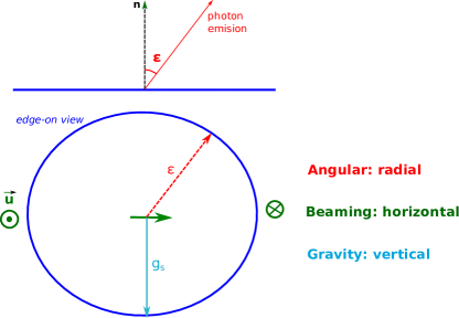
Figure 6: Sketch showing the main ingredients that explain the appearance of the star’s ray-traced image. The blue line represents the neutron star’s surface. The upper panel is a local view defining the emission angle $\epsilon$ between the local normal and the direction of photon emission. The lower panel shows an edge-on view of a rapidly rotating neutron star. Note that the surface is not a circle due to the high rotation. The value of $\epsilon$ varies radially for an exactly edge-on view. Its direction of increase is along the long dashed red arrow. The 4-vector of the neutron star’s surface velocity is labeled $\mathbf{u}$. Its spatial part $\vec{u}$ points towards the observer on the left side, lies in the plane of the paper at the center, and points away from the observer on the right side. The corresponding beaming effect will enhance the radiation on the left side and weaken the radiation on the right side. The beaming effect thus shows a horizontal gradient. The surface gravity $g_{\rm s}$ is minimum at the center of the picture (the starting point of the cyan arrow), as this point is the projection of some point in the equator of the star where the radius is maximum. On the other hand, $g_{\rm s}$ is maximum at the end point of the cyan arrow, which corresponds to a pole of the star, where the radius is minimum. Thus, $g_{\rm s}$ increases from the center of the image towards the border of the star, along the cyan vertical arrow. Surface gravity has constant values on horizontals in this picture, and thus shows a vertical gradient.

Fig. 7 shows the face-on and edge-on views of the non-rotating neutron star, together with the face-on view of the fast-rotating ($716$ Hz) star. We note that we call face-on view an image obtained with an inclination $i=1^{\circ}$. Our ray-tracing code uses spherical coordinates so that the $i=0^{\circ}$ axis is singular. We also note that the computation time of one such image (or spectrum) with resolution $30\times 30$ pixels on a standard laptop takes $\approx 5$ min, allowing to compute rather easily a large number of such images/spectra.

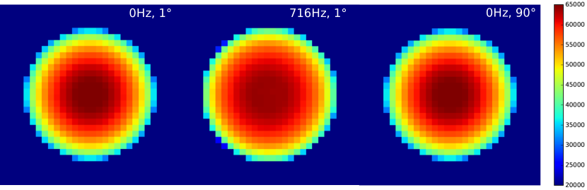
Figure 7: Images of the neutron star at observed energy $4.1$ keV with $(\Omega=0,i=1^{\circ})$ for the left panel, $(\Omega=716~{}\mathrm{Hz},i=1^{\circ})$ for the central panel, and $(\Omega=0,i=90^{\circ})$ for the right panel. The star is emitting the directional spectrum as computed by the Atm24 code in all cases. The mainly radial gradient of intensity is due to the radial variation of the emission angle $\epsilon$. The color bar is common to the three panels and shows the numerical value of the observed $I_{\nu}$ in cgs units.

Obviously, the face-on and edge-on views of the non-rotating star (left and right panels) are extremely similar. When comparing pixel by pixel, some non-negligible differences appear that can be as high as $\approx 1\%$ for a handful of pixels. This is due to the limited precision with which the Gyoto code is able to find the neutron star’s surface, in particular for tangential approach (remember that geodesics are integrated backwards in time, so the photon approaches the neutron star). The code precision parameters can be adjusted to allow obtaining an arbitrarily precise result, but at the expense of computing time. Given that the total flux, summed over all pixels, is the real quantity of interest, we are not interested in getting extremely precise values for each individual pixel. We have checked that the flux difference between the edge-on and face-on views of the non-rotating star is of $0.05\%$, which is far better than needed to fit observations. The mainly radial gradient of the intensity in these images is due to the radial variation of the emission angle $\epsilon$, as explained in Fig. 6. We have checked that the image obtained when the local spectrum is averaged over emission angle shows an exactly constant value to within code precision. The central panel of Fig. 7 is the face-on view of the fast-rotating star. It is very similar to the non-rotating neutron star image, which is natural as the main effect that differs when the star is rotating is the relativistic beaming effect, which is absent for a face-on view. The pixel values are still slightly different as compared to the non-rotating case because the metric felt by the ray-traced photons is different even for a face-on view, and the surface gravity is not exactly the same in both cases.

Fig. 8 shows edge-on images of the fast-rotating neutron star. We have considered three different emission processes at the star’s surface: either a simple color-corrected blackbody at $T=10^{7}$ K, with a color-correction factor of $f_{\mathrm{cor}}=1.4$, or the local spectrum as computed by the Atm24 code, averaged or not over the emission angle $\epsilon$.

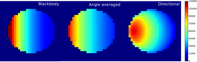
Figure 8: Edge-on images of the fast-rotating ($716~{}$Hz) star. On the left panel, the star emits a simple color-corrected blackbody at $T=10^{7}$ K. On the central panel, the star emits the spectrum computed by the Atm24 code, averaged over the emission angle $\epsilon$. The right panel shows the most realistic image with the directional spectrum as computed by Atm24 taken into account. The two first panels show a clear dominating horizontal gradient that is due to relativistic beaming. The right panel superimposes to this effect the radial gradient of the emission angle $\epsilon$, leading to a more complex appearance. The color bar is common to the three panels and shows the numerical value of the observed $I_{\nu}$ in cgs units. Note that the star’s surface is not circular due to the high rotation.

The left and central panels are very similar. They show a mainly horizontal gradient that is due to the relativistic beaming effect (the approaching side being on the left). The blackbody case shows no vertical gradient, to within the code precision. The averaged Atm24 spectrum case shows a very small vertical gradient (not visible on Fig. 8, the horizontal gradient largely dominates), that is due to the slight variation of the local spectrum with surface gravity. The right panel shows the combination of two effects: the horizontal gradient due to relativistic beaming, and the radial gradient due to the variation of the emission angle $\epsilon$. The superimposition of these two effects leads to a more complex image.

3.4 Ray-traced spectra

This Section investigates the end product of our numerical pipeline, i.e. the ray-traced neutron star spectra. All the spectra in this Section are computed with the same $30\times 30$ pixels resolution as the images presented in the previous Section. We checked by comparing to a $100\times 100$ resolution for one particular case that this resolution leads to an error smaller than $0.7\%$ over the full energy range.

3.4.1 Impact of the emission process

Let us first focus on the impact of the local radiation process at the neutron star’s surface on the end-product, ray-traced observed spectrum. Fig. 9 shows the ray-traced spectra of the non-rotating or fast-rotating neutron star for three different kinds of emissions at the star’s surface: either a color-corrected blackbody at the effective temperature of $T=10^{7}$ K, or the Atm24 spectrum averaged over emission angle, or the directional Atm24 spectrum.

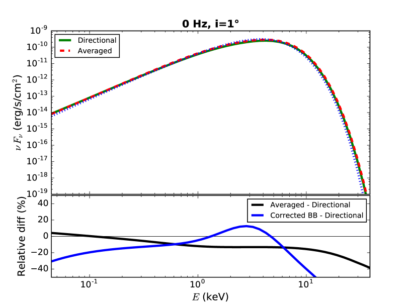
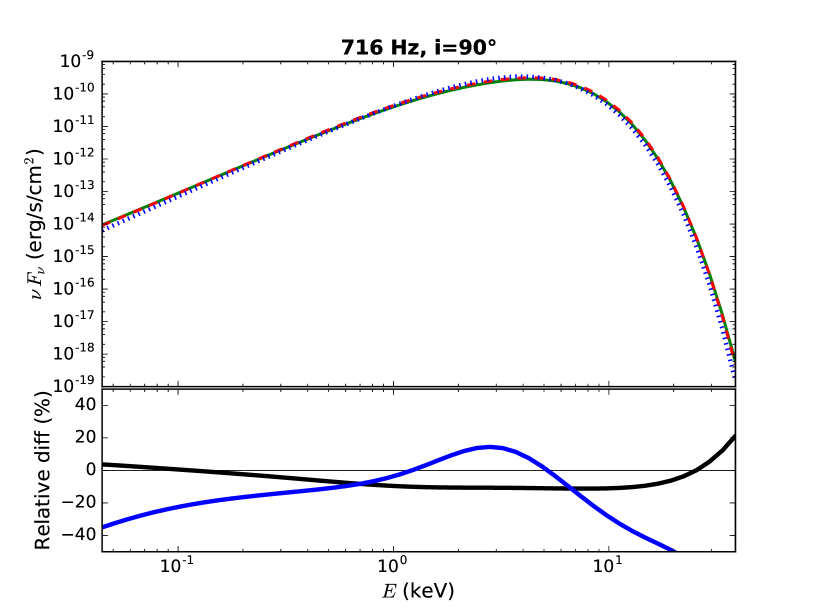
Figure 9: Effect of the emission process on the observed spectra: Top panel: ray-traced spectra (and relative differences) of a neutron star with zero rotation seen face on. Lower panel: same for a neutron star with $716$ Hz rotation seen edge on. Three different radiation processes are considered at the star’s surface: color-corrected blackbody at $T=10^{7}$ K (dotted blue), Atm24 spectrum averaged over emission angle (solid green), or Atm24 directional spectrum (dashed red). The lower sub-panel of each plot shows the relative difference in percentage between the averaged and directional Atm24 spectra (solid black), and between the corrected blackbody and the directional Atm24 spectrum (solid blue).

This Figure shows that the difference between the ray-traced spectra of a neutron star emitting a color-corrected blackbody or a realistic spectrum as computed by Atm24 is of the same order as what was obtained in the local context of Fig. 5. Thus, taking a realistic emitted spectrum into account changes the observed spectrum by typically $\approx 20\%$ over most of the energy band. This difference is related to the fact that the locally emitted spectrum is strongly directional. This directional dependence cannot be simplified, particularly when the star rotates fast and the photons undergo highly non-trivial lensing effects that impact their emission angle $\epsilon$, and thus the specific intensity they carry. We note that, as illustrated in Fig. 5, even the angle-averaged local spectrum is still very different from a corrected blackbody, so that even if one replaces the directional emitted spectrum by its angle average (which would be wrong, because of the non-trivial lensing effects highlighted before), the resulting ray-traced spectrum would still be incorrect. This problem is analogous to the computation of the spectra reflected by black holes’ accretion disks. Ray-tracing techniques must be used to compute the reflected spectrum in order to take properly into account the strong directional dependence of the local spectrum (García et al., 2014; Vincent et al., 2016).

Figure 9 also allows to compare the end-product ray-traced spectrum when averaging the Atm24 local spectrum over emission angle as compared to the directional case. This is particularly interesting as a test of our pipeline, because the result can be predicted to some extent. Let us first focus on the $(\Omega=0,i=1^{\circ})$ case (that is very similar to the $(\Omega=716~{}\mathrm{Hz},i=1^{\circ})$ case, which is thus not shown here). The relative difference between the ray-traced averaged and directional spectra is very similar to the relative difference between the local tangent and normal spectra of Fig. 5 (solid black, lower panel):

$$\underbrace{\mathrm{Averaged-Directional}}_{\mathrm{in\;ray-traced\;spectrum}}\approx\underbrace{\mathrm{Tangent-Normal}}_{\mathrm{in\;local\;spectrum}}.$$ (20)

The absolute value of the relative difference is smaller in the ray-traced case, but the trend is exactly the same, as if the directional ray-traced spectrum would privilege normal emission. It is indeed so, as illustrated on Fig. 10: the projection effect suffered by the star when it is imaged on a flat screen at the observer’s position

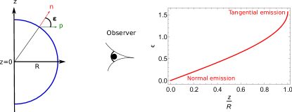
Figure 10: On the left, the star’s surface is shown in blue. The $z$ axis is the axis of rotation, $\mathbf{n}$ is the local normal at some point of the surface, $\mathbf{p}$ is the direction of emission towards the observer, $\epsilon$ is the emission angle, and $R$ the neutron star radius. The plot on the right shows the evolution of $\epsilon=\mathrm{arcsin}(z/R)$ with $z/R$. The emission is normal when $\epsilon=0$ and tangential when $\epsilon=\pi/2$. Because of the projection effect when imaging the neutron star on a screen at the observer’s location, more weight will be given to normal emission than to tangential emission. Indeed, a majority of values of $z/R$ give rise to values of $\epsilon$ that are closer to $0$ than to $\pi/2$, as is clear from the right panel.

leads to giving more weight to normal emission than to tangential emission. On the contrary, when considering an averaged spectrum, all values of $\epsilon$ are considered with the same weight. The trend of the top panel of Fig. 9 thus makes sense. Let us now focus on the lower panel of this Figure, i.e. the $(\Omega=716~{}\mathrm{Hz},i=90^{\circ})$ case. The relative difference between the averaged and directional ray-traced spectra is similar to the top panel on the low-energy side, but then gets inverted at high energies. This is linked to the relativistic beaming effect, which is the main effect shaping the edge-on spectra as illustrated in Fig. 8. However, the effect of beaming strongly depends on the spectrum’s slope. Let us illustrate this by focusing on the approaching side of the star (the left part of the image in Fig. 8). As the emitter travels towards the observer, the Doppler effect translates in the observed photon energy being higher than the emitted one. Thus, the Doppler effect pushes the emitted intensity towards smaller values when the spectrum increases with energy, and towards higher values when the spectrum decreases with energy (see Fig. 11).

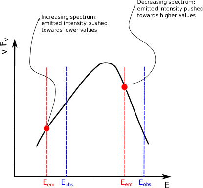
Figure 11: Illustration of the combination of Doppler and beaming effect depending on the spectral trend, on the approaching side of a neutron star observed edge-on. See text for details.

On the approaching side, the beaming effect has always the same effect, whatever the spectrum shape, it enhances the radiation. Consequently, Doppler effect tends to compensate the beaming effect on the increasing side of the spectrum (i.e. low-energy side), and to boost the beaming effect on the decreasing side of the spectrum (i.e. high-energy side). This allows to understand the trend of the relative difference between the averaged and directional spectra of the lower panel of Fig. 9. On the low-energy side, Doppler effect counterbalances the beaming effect so that things look very much like the face-on case which is not affected by beaming. On the contrary, on the high-energy side, Doppler effect increases the effect of beaming, strongly concentrating the radiation in the left-most part of the image. This part of the image is associated to mostly tangential emission as it lies far away from the center of the neutron star on the observer’s screen. Thus, the directional ray-traced spectrum selects tangential emission, the opposite as to what was the case in the face-on scenario discussed above. This explains the opposite trend of the relative difference plot in the lower panel of Fig. 9, as compared to the top one. Thus, all trends depicted on Fig. 9 can be explained. This is a strong argument in favor of the correctness of our pipeline.

3.4.2 Impact of the angular velocity

Figure 12 illustrates the effect of the star’s rotation on the observed ray-traced spectrum, when the neutron star emits either a color-corrected blackbody or the directional Atm24 spectrum.

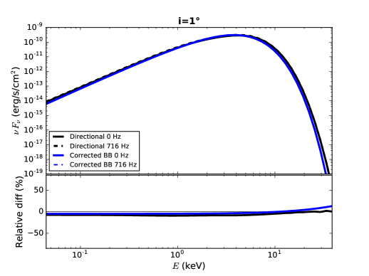
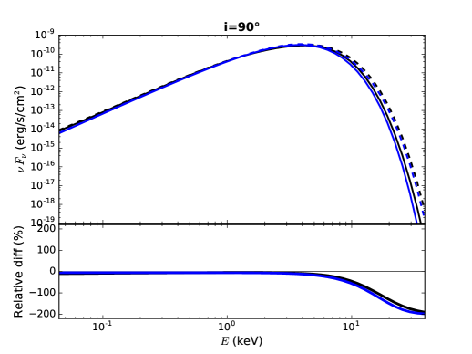
Figure 12: Effect of rotation on the observed spectrum: ray-traced spectra of a neutron star seen face on (left) or edge on (right). The star’s surface emits color-corrected blackbody (blue) or the directional Atm24 spectrum (black) and rotates at $0$ Hz (solid) or $716$ Hz (dashed). The lower panels show the relative difference between the two blackbody and directional spectra in blue and black respectively. Note the change of the vertical axis scale between the two lower panels.

It shows that the rotation has a small impact when the star is seen face on, which is not surprising after what has been discussed on Fig. 7. The difference is here purely due to the change of the spacetime metric with the star’s rotation. On the contrary, the effect of rotation is huge at high energy when the star is seen edge on, with a difference reaching factors of a few. However, this effect is still small, even for the edge-on case, on the low-energy side. This trend is explained in the same way as above, by the coupled influence of the Doppler and beaming effects. Fig. 12 also shows that the effect of rotation is very similar for the two different emission processes, blackbody and directional Atm24 spectrum.

The bolometric flux relative difference between the $0$ Hz and $716$ Hz cases, for edge-on view, is of $13.7\%$ for the blackbody case, and $11.2\%$ for the Atm24 case. These numbers are difficult to directly compare to the results of Bauböck et al. (2015) given that the neutron star’s parameters are not the same. However, we note that the bolometric relative difference reported by these authors between a $15$ km neutron star rotating at $\approx 700$ Hz and its non-rotating counterpart, seen edge-on, is of $\approx 15\%$ according to their Fig. 4, lower panel.

4 Conclusions

We have presented a new numerical pipeline that intends to compute very accurate X-ray bursting spectra of neutron stars, for arbitrary masses and rotation. It is the only tool in the literature, so far, that allows to compute neutron-star spectra considering realistic model atmospheres together with all general-relativistic effects on the star’s shape and photon propagation. Our pipeline is the concatenation of the Lorene/nrotstar code together with the Atm24 and Gyoto codes. At the present time, only Lorene/nrotstar and Gyoto are fully open-source, but we consider making Atm24 open-source in the close future, so that the pipeline can be freely used by the community.

This article first demonstrates the validity of our pipeline by investigating in detail its outputs and comparing them when possible to the literature. It also highlights the importance of considering both a precise directional model atmosphere and ray tracing in order to obtain accurate predictions.

Our future work will be dedicated to broadening the astrophysical impacts of this new pipeline, making it a testbed to investigate the validity of the various simplifying assumptions, either on the emitted spectrum or on the treatment of strong gravity, that other codes consider. The output of the pipeline will be implemented in xspec by creating fits tables of bursting neutron star spectra that might then be easily used for fitting data. Finally, we identify potentially interesting research directions that can be only undertaken with such a fully relativistic pipeline, namely detailed investigation of the impact of the dense matter EoS on the observables. We will also consider ”extreme” neutron stars, both very massive and fast-rotating, in order to predict the observable specific features of these very special sources.

Appendix A Validity of Atm24 code

Numerical solution of the model atmosphere problem is very time consuming. We assume, that each model fulfills the conditions of radiative and hydrostatic equilibrium, which determines the evolution of temperature and gas pressure in the atmosphere. These two conditions are numerically achieved by means of iterations, with gas pressure iterations being nested in temperature iterations.

Atm24 uses very efficient and fast algorithms to ensure hydrostatic equilibrium. However, temperature iteration steps are very slow and must be repeated hundreds of times in the most complicated models. In a typical computation, each step requires solving 1025 (i.e. the number of frequencies) integro-differential equations of transfer with Compton redistribution function at all optical depth levels (typically 96 levels).

The Atm24 code is constantly upgraded to increase its accuracy. The most difficult case is the pure hydrogen atmosphere, when matter is completely ionized and Compton scattering is the dominant process of opacity. Furthermore, the convergence problem appears when the surface gravity is close to the Eddington limit, above which the atmosphere becomes unstable.

Recently Suleimanov et al. (2012) pointed out that our code Atm24 is not correct on the basis of a single result, which was exchanged with those authors by us in private communication. This result was obtained for a pure hydrogen atmosphere, with parameters close to the Eddington limit $T_{\rm eff}=1.80\times 10^{7}$ K and $\log g=14.0$ (cgs units). Even if flux and temperature corrections were iterated with the accuracy of 0.1% the final spectral shape was not converged yet (after 62 temperature iterations, which we normally have used for testing purposes). In Fig. 13 we show also subsequent iterations, 264 and 1954, of the same model atmosphere computed with the same version of Atm24 code as quoted by Suleimanov et al. (2012). The above figure shows significant evolution of the model spectrum reaching the convergence limit of about 2000 iterations. For models with higher surface gravity (i.e. far from Eddington limit) usually less than 600 iterations are sufficient to achieve satisfactory convergence. The remaining difference with respect to Suleimanov et al. (2012) is displayed at the bottom panel of Fig. 13.

Therefore, the fully iterated sample Atm24 model is also in agreement with Boutloukos et al. (2010) and Miller et al. (2011), who concluded that the brightest RXTE spectra of X-ray bursters 4U 1820-30 and GX 17+2 are best fitted by Bose-Einstein spectra possibly with nonzero chemical potential.

We note, that the spectral shape computed with Atm24 code and discussed by Suleimanov et al. (2012) and by Medin et al. (2016) was neither published nor endorsed for publication by our group in any of our earlier papers. The differences between models computed by different groups may be caused by the use of different algorithms or computational schemes since the problem is very complex and requires huge CPU time. A more detailed comparison of Atm24 models and those of Suleimanov et al. (2012) will be presented in a forthcoming paper, Madej et al. (2018, in prep.).

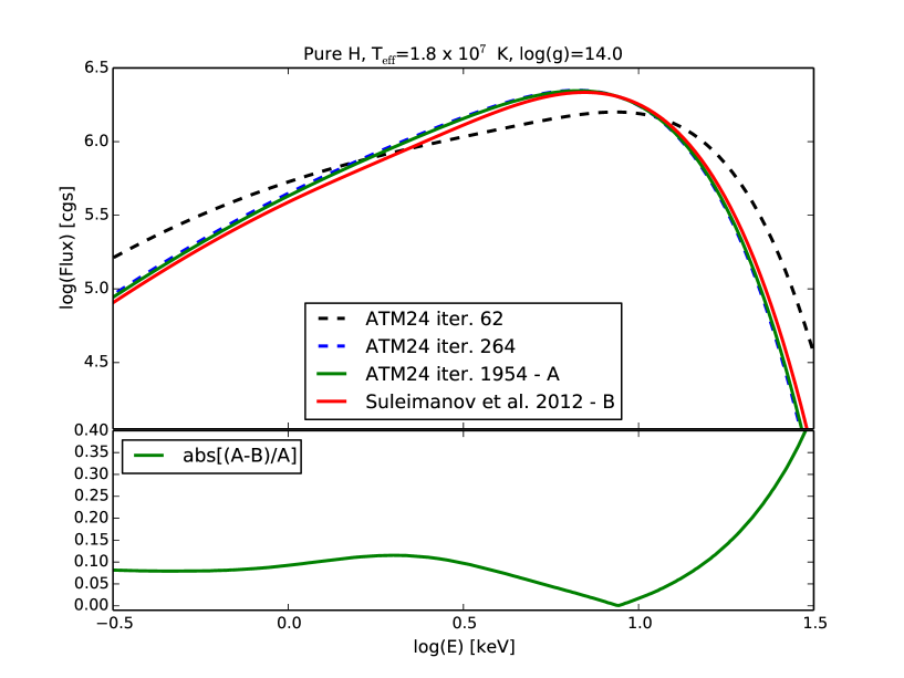
Figure 13: The convergence of Atm24 code for pure hydrogen atmosphere. The dashed black line shows the spectrum after 62 iterations, which is not fully converged, and was used in the comparison of Fig. C.1 of Suleimanov et al. (2012). Increasing the number of iterations to 264 and 1954 respectively gives the dashed blue and solid green lines. These spectra show perfect convergence of spectral shape and are compared to the spectrum computed by Suleimanov et al. (2012) numerical code (solid red line). The comparison shows a very good agreement at the few percent level around the spectrum maximum.

References

- Abbott et al. (2017a) Abbott, B. P., Abbott, R., Abbott, T. D., Acernese, F., et al. 2017a, Phys. Rev. Lett., 119, 161101. https://link.aps.org/doi/10.1103/PhysRevLett.119.161101
- Abbott et al. (2017b) —. 2017b, The Astrophysical Journal Letters, 848, L12. http://stacks.iop.org/2041-8205/848/i=2/a=L12
- Abbott et al. (2017c) —. 2017c, The Astrophysical Journal Letters, 848, L13. http://stacks.iop.org/2041-8205/848/i=2/a=L13
- Arnaud (1996) Arnaud, K. A. 1996, in Astronomical Society of the Pacific Conference Series, Vol. 101, Astronomical Data Analysis Software and Systems V, ed. G. H. Jacoby & J. Barnes, 17
- Arnowitt et al. (1961) Arnowitt, R., Deser, S., & Misner, C. W. 1961, Phys. Rev., 122, 997. https://link.aps.org/doi/10.1103/PhysRev.122.997
- Bauböck et al. (2013) Bauböck, M., Berti, E., Psaltis, D., & Özel, F. 2013, ApJ, 777, 68
- Bauböck et al. (2015) Bauböck, M., Özel, F., Psaltis, D., & Morsink, S. M. 2015, ApJ, 799, 22
- Bauböck et al. (2012) Bauböck, M., Psaltis, D., Özel, F., & Johannsen, T. 2012, ApJ, 753, 175
- Bejger & Haensel (2004) Bejger, M., & Haensel, P. 2004, A&A, 420, 987
- Berti et al. (2005) Berti, E., White, F., Maniopoulou, A., & Bruni, M. 2005, MNRAS, 358, 923
- Boutloukos et al. (2010) Boutloukos, S., Miller, M. C., & Lamb, F. K. 2010, ApJ, 720, L15
- Cadeau et al. (2005) Cadeau, C., Leahy, D. A., & Morsink, S. M. 2005, ApJ, 618, 451
- Cadeau et al. (2007) Cadeau, C., Morsink, S. M., Leahy, D., & Campbell, S. S. 2007, ApJ, 654, 458
- Chabanat et al. (1998) Chabanat, E., Bonche, P., Haensel, P., Meyer, J., & Schaeffer, R. 1998, Nuclear Physics A, 635, 231
- Douchin & Haensel (2001) Douchin, F., & Haensel, P. 2001, A&A, 380, 151
- Fujimoto & Taam (1986) Fujimoto, M. Y., & Taam, R. E. 1986, ApJ, 305, 246
- García et al. (2014) García, J., Dauser, T., Lohfink, A., et al. 2014, ApJ, 782, 76
- Gourgoulhon (2010) Gourgoulhon, E. 2010, ArXiv e-prints, arXiv:1003.5015
- Gourgoulhon et al. (2016) Gourgoulhon, E., Grandclément, P., Marck, J.-A., Novak, J., & Taniguchi, K. 2016, LORENE: Spectral methods differential equations solver, Astrophysics Source Code Library, , , ascl:1608.018
- Guillot et al. (2011) Guillot, S., Rutledge, R. E., & Brown, E. F. 2011, ApJ, 732, 88
- Haensel et al. (2016) Haensel, P., Bejger, M., Fortin, M., & Zdunik, L. 2016, European Physical Journal A, 52, 59
- Haensel & Pichon (1994) Haensel, P., & Pichon, B. 1994, A&A, 283, 313
- Haensel et al. (2007) Haensel, P., Potekhin, A. Y., & Yakovlev, D. G. 2007, Astrophysics and Space Science Library, Vol. 326, Neutron Stars 1 : Equation of State and Structure
- Hartle & Thorne (1968) Hartle, J. B., & Thorne, K. S. 1968, ApJ, 153, 807
- Heinke et al. (2006) Heinke, C. O., Rybicki, G. B., Narayan, R., & Grindlay, J. E. 2006, ApJ, 644, 1090
- Hessels et al. (2006) Hessels, J. W. T., Ransom, S. M., Stairs, I. H., et al. 2006, Science, 311, 1901
- Kuśmierek et al. (2011) Kuśmierek, K., Madej, J., & Kuulkers, E. 2011, MNRAS, 415, 3344
- Madej (1989) Madej, J. 1989, ApJ, 339, 386
- Madej (1991a) —. 1991a, Acta Astron., 41, 73
- Madej (1991b) —. 1991b, ApJ, 376, 161
- Madej et al. (2004) Madej, J., Joss, P. C., & Różańska, A. 2004, ApJ, 602, 904
- Madej et al. (2017) Madej, J., Różańska, A., Majczyna, A., & Należyty, M. 2017, MNRAS, 469, 2032
- Majczyna & Madej (2005) Majczyna, A., & Madej, J. 2005, Acta Astron., 55, 349
- Majczyna et al. (2005) Majczyna, A., Madej, J., Joss, P. C., & Różańska, A. 2005, A&A, 430, 643
- Medin et al. (2016) Medin, Z., von Steinkirch, M., Calder, A. C., et al. 2016, ApJ, 832, 102
- Mihalas (1978) Mihalas, D. 1978, Stellar atmospheres /2nd edition/
- Miller (2013) Miller, M. C. 2013, ArXiv e-prints, arXiv:1312.0029
- Miller et al. (2011) Miller, M. C., Boutloukos, S., Lo, K. H., & Lamb, F. K. 2011, in Fast X-ray Timing and Spectroscopy at Extreme Count Rates (HTRS 2011), 24
- Miller & Lamb (2016) Miller, M. C., & Lamb, F. K. 2016, European Physical Journal A, 52, 63
- Nagirner & Poutanen (1993) Nagirner, D. I., & Poutanen, Y. J. 1993, Astronomy Letters, 19, 262
- Nättilä et al. (2017) Nättilä, J., Miller, M. C., Steiner, A. W., et al. 2017, ArXiv e-prints, arXiv:1709.09120
- Nättilä & Pihajoki (2017) Nättilä, J., & Pihajoki, P. 2017, ArXiv e-prints, arXiv:1709.07292
- Özel & Freire (2016) Özel, F., & Freire, P. 2016, ARA&A, 54, 401
- Özel et al. (2009) Özel, F., Güver, T., & Psaltis, D. 2009, ApJ, 693, 1775
- Özel et al. (2016) Özel, F., Psaltis, D., Güver, T., et al. 2016, ApJ, 820, 28
- Pomraning (1973) Pomraning, G. C. 1973, The equations of radiation hydrodynamics
- Sampson (1959) Sampson, D. H. 1959, ApJ, 129, 734
- Stergioulas & Friedman (1995) Stergioulas, N., & Friedman, J. L. 1995, ApJ, 444, 306
- Suleimanov et al. (2011) Suleimanov, V., Poutanen, J., & Werner, K. 2011, A&A, 527, A139
- Suleimanov et al. (2012) —. 2012, A&A, 545, A120
- Suleimanov et al. (2016) Suleimanov, V. F., Poutanen, J., Klochkov, D., & Werner, K. 2016, European Physical Journal A, 52, 20
- van Paradijs (1979) van Paradijs, J. 1979, ApJ, 234, 609
- van Paradijs & Lewin (1987) van Paradijs, J., & Lewin, W. H. G. 1987, A&A, 172, L20
- Vincent et al. (2012) Vincent, F. H., Gourgoulhon, E., & Novak, J. 2012, Classical and Quantum Gravity, 29, 245005
- Vincent et al. (2011) Vincent, F. H., Paumard, T., Gourgoulhon, E., & Perrin, G. 2011, Classical and Quantum Gravity, 28, 225011
- Vincent et al. (2016) Vincent, F. H., Różańska, A., Zdziarski, A. A., & Madej, J. 2016, A&A, 590, A132
- Webb & Barret (2007) Webb, N. A., & Barret, D. 2007, ApJ, 671, 727
- Zdunik et al. (2006) Zdunik, J. L., Bejger, M., Haensel, P., & Gourgoulhon, E. 2006, A&A, 450, 747