Information and Coarse-Graining in Eternal Black Holes

Dongsu Bak

Physics Department, University of Seoul, Seoul 02504 KOREA

(dsbak@uos.ac.kr)

ABSTRACT

Recently it was shown in the context of the AdS/CFT correspondence that the classical gravity description inevitably involves coarse-graining of some degrees. In this note we clarify the nature of this coarse-graining both in gravity and field theory sides. We show that the information carried by the bulk classical gravity fluctuation is transferred to the coarse-grained nonclassical degrees through tiny interactions, which makes the recovery of information almost impossible. Of course, the total system is evolving unitarily fully preserving its information as dictated by the basic construct of the AdS/CFT correspondence.

1 Introduction

Based on the AdS/CFT correspondence [1, 2, 3], one may study bulk gravity dynamics in a rather precisely defined setup. Numerous aspects of the correspondence have been checked for many examples in the zero temperature limit and well understood by now. In this non thermal regime, there are no conceptual issues such as non-unitarity of description. On the other hand, a precise understanding of the gravity description of thermal field theories is still lacking, which is relevant to the problem of the black hole information paradox [4].

In Ref. [5], rather general perturbations of BTZ black hole [6] are constructed which are dual to state deformations of the thermofield double theory [7]. This construction may be viewed as a realization of micro thermofield deformations of the BTZ geometry and may serve as an ideal setup to clarify the issues of black hole dynamics in AdS spacetime. The perturbation makes one-point function of operator nonvanishing initially. This one-point function decays exponentially in general, which is contradicting with the unitarity of the CFT defined on $R\times S^{d-1}$. Furthermore the future horizon area of this classical geometry grows in time in general. Interpretation of the corresponding geometric entropy is the key issue which we would like to address in this note. We would like to clarify the nature of gravity description by investigating the degrees relevant to the growing of gravitational entropy.

In short, the gravity description of thermal field theories naturally involves a coarse-graining of certain degrees. We identify the coarse-grained degrees as nonclassical degrees such as Hawking radiation quanta, which cannot be seen in the classical gravity description. The interaction between the classical gravity degrees with these coarse-grained nonclassical degrees is tiny but nonvanishing and hence they work as a dark sector from the view point of the classical gravity description. In this note, we shall describe the development of entanglement between the two and transfer of information from the classical gravity to the coarse-grained degrees. We shall also discuss how one can regain the unitarity from the view points of both the gravity and the boundary field theory.

In section 2, we review the general perturbations of BTZ background studied in Ref. [5] and the corresponding AdS/CFT correspondence [8]. The basic puzzles of entropy and unitarity of the gravity description are described in detail. We clarify the degrees responsible for coarse-graining of bulk gravity description. In section 3, we present a field theory model to explain the entropy growth of the perturbation as forming entanglement between the classical gravity and the coarse-grained degrees. We also discuss how one can regain unitarity in this model. In section 4, we explain what happens from the bulk view point. This represents the quantum version of ER = EPR [9, 10, 11] where ER bridges are formed between the classical and nonclassical degrees. The latter degrees cannot be seen from the view point of the classical gravity description.

2 Eternal black holes and perturbation of states

The eternal black hole in AdS spacetime is dual to the thermofield double of a CFT, which is maximally entangled but non interacting [8]. The Hamiltonian of the total system is given by

$$H_{tfd}=H_{L}+H_{R}=H\otimes 1+1\otimes H$$ (2.1)

where there are absolutely no interactions between the left and the right CFT’s. We denote the CFT Hamiltonian by $H$. The initial unperturbed thermal vacuum state is given by a particularly prepared entangled state

$$|\Psi(0)\rangle=\frac{1}{\sqrt{Z}}\sum_{n,n^{\prime}}\,\langle n|U|n^{\prime}\rangle\,|n^{\prime}\rangle\otimes|n\rangle=\frac{1}{\sqrt{Z}}\sum_{n}\,e^{-\frac{\beta}{2}E_{n}}\,|n\rangle\otimes|n\rangle$$ (2.2)

with a Euclidean evolution operator $U=U_{0}=e^{-\frac{\beta}{2}H}$ and $Z$ denoting the normalization constant. The entanglement here is maximal for a given temperature $T=1/\beta$. In Figure 1, we illustrate the Penrose diagram of the corresponding BTZ black hole in three dimensions where two boundary spacetimes connected though an ER bridge representing the left-right entanglement. Here two copies of a 2d CFT live on the left and the right boundary spacetimes respectively.

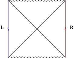
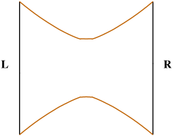
Figure 1: On the left, the Penrose diagram of the BTZ black hole is depicted. Two copies of a CFT live in the left and the right boundaries denoted by $L$ and $R$ respectively. On the right, we draw the ER bridge connecting the two boundaries. The left-right entanglement equals to the ER bridge of BTZ black hole connecting the left and the right boundaries.

This BTZ initial state can be deformed by introducing a mid-point insertion of operators as

$$U=e^{-\frac{\beta}{4}H}e^{-\sum_{k}c_{k}O_{k}}e^{-\frac{\beta}{4}H}$$ (2.3)

where $O_{k}$ denote general operators of the underlying CFT [5]. Then we evolve the system in time in a standard manner as

$$|\Psi(t)\rangle=e^{-iH_{tfd}\,t}\,|\Psi(0)\rangle$$ (2.4)

The one-point function

$$\langle O_{R}\rangle=\langle\Psi(t)|1\otimes O|\Psi(t)\rangle$$ (2.5)

was computed in [5] to the leading order in its coefficient $c_{k}$ using the conformal perturbation theory and the two-point function [14, 8]

$$\frac{1}{Z}{\rm tr}O(t,\varphi)O(t^{\prime},\varphi^{\prime})e^{-\beta H}=\sum^{\infty}_{m=-\infty}\frac{{\cal N}_{\Delta}}{\left[\cosh\frac{2\pi}{\beta}(t-t^{\prime})-\cosh\frac{2\pi\ell}{\beta}(\varphi-\varphi^{\prime}+2\pi m)-i\epsilon\right]^{\Delta}}$$ (2.6)

where $\Delta$ is the dimension of the scalar primary operator $O$ and ${\cal N}_{\Delta}$ [15] is an appropriate normalization. Here for the sake of an illustration, we consider 2d CFT on $R\times S^{1}$ where we use coordinates $(t,\varphi)$ with $\varphi\sim\varphi+2\pi$. (Of course, our presentation can be generalized to other dimensions in a straightforward manner.) Then the field theory result agrees with the holographic computation of one-point function precisely [5]. One finds that the resulting expression decays exponentially in time, which contradicts with the quantum Poincare recurrence theorem [16]. Indeed the above expression of the two-point function is not exact but involves a large $N\,(\sim 1/\sqrt{G\ell^{1-d}})$ approximation. To understand this classical gravity approximation, we need to clarify the nature of the above large $N$ limit in the dual field theories.

Next we discuss the issue of entropy involved with the above deformations. Let us first introduce the reduced density matrix

$$\rho_{R}(t)={\rm tr}_{L}\,|\Psi(t)\rangle\langle\Psi(t)|$$ (2.7)

and then the corresponding von Neumann entropy

$$S_{R}=-{\rm tr}_{R\,}\rho_{R}(t)\log\rho_{R}(t)$$ (2.8)

gives us an entanglement measure of the left-right system. The perturbation in the above makes this left-right entanglement non-maximal initially. One finds this L-R entanglement is time independent since one may undo the similarity transformation of the time evolution of the reduced density matrix inside the trace. Since there are no interactions between the left right system, any net information of one side cannot be transferred to the other side. This is consistent with the causal structure of the eternal black hole spacetime where the left and the right boundaries are causally disconnected from each other.

In Ref.  [5], it was also shown that, for any perturbation of initial state in (2.2), there exists a corresponding one-to-one deformation of the eternal black hole spacetime. See Figure 2 for a Penrose diagram of perturbed BTZ black hole. These geometries show two general features. Any initial perturbations decay exponentially in time with the time scale of so called relaxation time scale $\beta$. In the gravity side, the perturbation outside horizon generically falls into the horizon and the corresponding horizon perturbations decay away exponentially in the time scale of the relaxation time scale. This is generic in thermal AdS spacetime. With black holes, the decay is explained by the physics of quasi-normal modes which makes any perturbations of the black horizon decay away exponentially. This is consistent with the field theory result using the large $N$ approximation in (2.6).

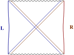
Figure 2: Penrose diagram of perturbed BTZ black hole is depicted here. The Hamiltonian of the system is not perturbed but only initial state is perturbed in a non maximally entangled manner. The diagram is elongated horizontally in such a way that the two sides are causally disconnected.

The second is regarding entropy whose precise nature is our primary concern in this note. In geometric side, the leading order gravitational entropy is given by the horizon area divided by $4G$. For instance we take the view point of the bulk observer outside of the future horizon from the right. The future horizon is nondecreasing monotonically in time reaching its asymptotic value after scrambling of the initial perturbation where the change of area $\Delta A$ is given by

$$\Delta A=A(\infty)-A(0)$$ (2.9)

which is finite and the function of the coefficients $c_{k}$. In the corresponding gravitational entropy is given by

$$S_{grav}(t)=\frac{A(t)}{4G}+S_{\delta}(t)$$ (2.10)

where $S_{\delta}$ denotes the contribution of order $G^{0}$ such as bulk entanglement entropy [17] which may be ignored in our discussion. In the late time, the area approaches its final value $A(\infty)$ exponentially in time again with the relaxation time scale. This leading term is the classical gravity contribution. It is rather clear that this entropy cannot be identified with the L-R entanglement entropy introduced in the above. The L-R entanglement entropy is time independent whereas the above is time dependent.

Understanding these two aspects will be our primary concern of this note. As was already noted in [12], these two at least indicate that the classical gravity description cannot be fully fine-grained. If it were fully fine-grained, the exponential decay of perturbation is not possible since it is contradicting with the quantum Poincare recurrence theorem [16]. It is also contradicting with the time independence of the L-R entanglement entropy which is dictated by the unitarity of the underlying system. Therefore it is rather clear that the classical gravity description cannot be fully fine-grained. This certainly implies that the classical gravity description is involving an inevitable coarse-graining. In this note, we would like to clarify the nature of gravity description in this respect. Of course the gravity description involves a large $N$ (or large central charge) approximation but the main question is which and how degrees are coarse-grained in the gravity description. We shall not be fully general here and our main focus is on the perturbations around thermofield double state. The unperturbed case corresponds to the BTZ spacetime, which involves a maximal entanglement between the left and right system leading to an equilibrium finite-temperature thermal system from the view point of one-sided observer. The perturbations then make the system non-maximally entangled.

We divide each-sided system by $B$ and $C$ where $B$ is for the degrees responsible for the bulk classical gravity and $C$ the system of the remaining degrees that are coarse-grained by the classical gravity description. Let us choose the right-side CFT whose Hamiltonian is given by $H$ in the above. The part $C$ is the complement of $B$ with $R=B+C$ and forms an environment of $B$ in some sense. There has to be nonvanishing interactions between $B$ and $C$. If there were no interactions, then the entropy would be time independent after integrating out those degrees of $C$. The interaction has to be as weak as $O(1/N)$. Otherwise it should be visible from the view point of the classical gravity.

The part $C$ here is describing the quantum gravity degrees such as Hawking radiation of quanta whose existence is invisible from the view point of the classical gravity. These include any of nonclassical degrees which are produced by $O(1/N)$ interactions. Namely for instance one cannot see any classical signal of such quanta from the BTZ background though their mass may be included into the definition of the energy of the dual field theory. Then $B$ is representing the part described by the classical gravity fluctuations. In this context, we shall refer the degrees of $C$ as nonclassical cloud (NCC) degrees, which are coarse-grained from the view point of classical gravity description. These degrees will be in thermal equilibrium with the black hole states forming a quantum cloud around the black hole since there is no net radiation for the case of BTZ black hole or the large AdS Schwarzschild black hole of other dimensions in general. Below we shall present such a model of coarse-graining degrees and explain the above two characteristics of the eternal black hole dynamics.

3 Field theory model

In this section, we model the above phenomena observed in the gravity side. As we described already, $B$ is representing the part described by the bulk fluctuation of the classical gravity that is one-to-one correspondence with the boundary deformation of the thermofield initial state with mid-point insertion of CFT operators. These operators are basically dual to those bulk fields, which are basic elements of the gravity description. We shall represent the corresponding field-theory fluctuation above the thermofield vacuum by

$$|\psi_{B}\rangle=\sum_{i}\alpha_{i}|i\rangle$$ (3.1)

where $|i\rangle$ is the eigenstate of $H_{B}$ with eigenvalue $\epsilon_{i}$ with $i=1,2,\cdots$. The coarse-grained degrees in $C$ are responsible for the Poincare recurrence to happen in the full system $R=B+C$. These degrees are excited in the black hole phase nonclassically forming the Hawking radiation cloud as we described previously. In the zero temperature limit, basically one may ignore these degrees since their occupation numbers are practically zero. Hence the effect of $C$ disappears in the zero temperature limit. It is not directly to do with higher derivative corrections since those higher derivative corrections are classical, which are well controlled in the AdS/CFT correspondence. Thus these higher derivative corrections will be included into the part $B$ of the classical gravity.

Our assumption is rather mild here. First of all, the interaction between $B$ and $C$ has to be extremely weak. Hence the degrees in $E=L+C$ should work as a dark sector from the view point of the gravity system $B$ where the left side $L$ is completely dark. In the zero temperature limit of non thermal field theories, the occupation number of NCC degrees vanishes and their effect can be ignored completely. This is why the gravity description in the zero temperature limit is unitary and fully fine-grained. On the other hand, at finite temperature, the number of excited NCC degrees in $C$ can be estimated as of order $N^{0}$ due to their semi-classical nature, which turns out to be still large enough. Thus many such NCC degrees are excited which we label by $I=1,2,\cdots,N_{s}$. The number of relevant states for the full environment of $E=L+C$ is of order $M^{N_{s}}\sim e^{\alpha N^{2}}$ where we assume there are $M$ states for each NCC degree.

Then, for the $I$-th NCC degree, the relevant state is given by

$$|\psi\rangle_{I}=\sum^{M}_{m=1}c^{I}_{m}\,|m\rangle_{I}$$ (3.2)

where we use the basis defined by $H_{I}|m\rangle_{I}=\frac{1}{M}e_{m}|m\rangle_{I}$ where $M$ is as large as $M\sim e^{\alpha N^{2}/N_{s}}$. The full relevant Hilbert space will be described by the tensor product

$$|\psi_{E}\rangle=\prod^{N_{s}}_{I=1}|\psi\rangle_{I}$$ (3.3)

We take the initial state of $E$ as

$$|\psi\rangle_{I}(0)=\frac{1}{\sqrt{M}}\sum^{M}_{m=1}e^{i\varphi^{I}_{m}}\,|m\rangle_{I}$$ (3.4)

with random phases $\varphi^{I}_{m}$ where all eigenstates are equally probable. The interaction Hamiltonian is given by

$$H_{int}=\frac{g_{0}}{N^{\prime}}H_{B}\otimes\sum_{I}H_{I}$$ (3.5)

where we assume that $N^{\prime}$ goes to infinity as $N_{s}$ tends to infinity. We shall assume that $H_{B}$ responsible of interactions is non-degenerate. Thus we begin with an initial state

$$\sum_{i}\alpha_{i}\,|i\rangle\otimes|\psi_{E}\rangle(0)$$ (3.6)

The entanglement entropy between $B$ and $E$ is zero since the reduced density matrix tracing over $E$ is still pure. Then the time evolution of the system is given by

$$\sum_{i}\alpha_{i}\,|i\rangle\otimes|\psi^{i}_{E}\rangle(t)$$ (3.7)

where one has

$$|\psi^{i}_{E}\rangle(t)=\prod^{N}_{I=1}|\psi^{i}\rangle_{I}(t)$$ (3.8)

with

$$|\psi^{i}\rangle_{I}(t)=\frac{1}{\sqrt{M}}\sum^{M}_{m=1}e^{i\varphi^{I}_{m}-i\frac{g_{0}\epsilon_{i}e_{m}}{N^{\prime}M}t}\,|m\rangle_{I}$$ (3.9)

Then the overlap can be evaluated as

$$\langle\psi^{i}|\psi^{j}\rangle_{I}=\frac{1}{M}\sum^{M}_{m=1}e^{ig_{0}\frac{\epsilon_{i}-\epsilon_{j}}{N^{\prime}}\frac{e_{m}}{M}t}$$ (3.10)

Since $M$ is large enough, we can turn this to an integral

$$\langle\psi^{i}|\psi^{j}\rangle_{I}=\int^{\infty}_{-\infty}dx\,D(x)\,e^{ig_{0}\frac{\epsilon_{i}-\epsilon_{j}}{N^{\prime}}xt}$$ (3.11)

where we introduce the normalized density of state $D(x)$ by

$$D(x)=\frac{1}{M}\sum^{M}_{m=1}\delta\Big{(}x-\frac{e_{m}}{M}\Big{)}$$ (3.12)

which satisfies the normalization

$$\int^{\infty}_{-\infty}dx\,D(x)=1$$ (3.13)

For instance choosing $D(x)=D_{0}(x)=\frac{1}{2\pi}\Theta(\pi-x)\Theta(x+\pi)$ leads to

$$\langle\psi^{i}|\psi^{j}\rangle_{I}=\frac{\sin\pi\frac{\epsilon_{i}-\epsilon_{j}}{N^{\prime}}g_{0}t}{\pi\frac{\epsilon_{i}-\epsilon_{j}}{N^{\prime}}g_{0}t}$$ (3.14)

This leads to the overlap

$$\langle\psi_{E}^{i}|\psi_{E}^{j}\rangle=e^{-\frac{\pi^{2}}{6}(\epsilon_{i}-\epsilon_{j})^{2}g_{0}^{2}t^{2}}$$ (3.15)

where we assume $N_{s}={N^{\prime}}^{2}$ and take the large $N_{s}$ limit. This decay rate is too fast since in the gravity side we have just exponential decay rate in the late time. Hence this example is not consistent with our bulk gravity dynamics described in section 2.

In this example, let us take $M$ and $N^{\prime}$ to be finite and further assume $M$ is even integer. By taking $e_{m}=m-M/2$ and $\epsilon_{i}=i$, one finds $D(x)=D_{0}(x)$ in the large $M$ limit. With this choice of $e_{m}$ and $\epsilon_{i}$, the state in (3.9) will return to its initial state as

$$|\psi^{i}\rangle_{I}(0)=|\psi^{i}\rangle_{I}(t_{rec})$$ (3.16)

where $t^{E}_{rec}=\pi N^{\prime}M/g_{0}$ with $t^{E}_{rec}$ denoting the Poincare recurrence time of the system. If one allows a slight random variation of multiplicity $M$ over $I$ with its mean value $\langle M\rangle=e^{\alpha N^{2}/N_{s}}$ and assumes $N^{\prime}=N_{s}$, the recurrence time scale becomes $t^{E}_{rec}\sim e^{N_{s}\log N_{s}}e^{\alpha N^{2}}\sim e^{S_{E}}$.

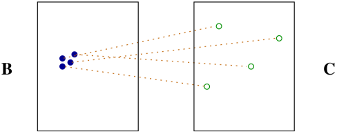
Figure 3: $B$ and $C$ represent respectively the classical gravity degrees and the remaining nonclassical degrees in $R$. EPR pairs between $B$ and $C$ are formed by entanglement, which are represented by the dotted lines. The interaction is small and the location of degrees in $C$ are random and $C$ is embedded in $E$.

To consider a more realistic case, we choose

$$D(x)=\frac{1}{\pi}\frac{a_{0}}{x^{2}+a_{0}^{2}}$$ (3.17)

together with $N^{\prime}=N_{s}$. Then one has

$$\langle\psi^{i}|\psi^{j}\rangle_{I}=e^{-|\frac{\epsilon_{i}-\epsilon_{j}}{N^{\prime}}a_{0}g_{0}t|}$$ (3.18)

This leads to the overlap

$$\langle\psi_{B}^{i}|\psi_{B}^{j}\rangle=e^{-|(\epsilon_{i}-\epsilon_{j})a_{0}g_{0}t|}$$ (3.19)

This is describing a typical decoherence [18] and consistent with the late time behavior of the perturbations in [5]. We take $a_{0}$ to be an order of typical thermal energy scale as $a_{0}=b_{0}T$. For example consider the case

$$|\psi_{B}\rangle=\frac{1}{\sqrt{2}}\big{(}|0\rangle+|1\rangle\big{)}$$ (3.20)

Then the reduced density matrix is obtained as

$$\rho_{B}=\frac{1}{2}\Big{[}|0\rangle\langle 0|+|1\rangle\langle 1|+\chi(t)(|0\rangle\langle 1|+|1\rangle\langle 0|)\Big{]}$$ (3.21)

where $\chi(t)=e^{-k_{0}\frac{t}{\beta}}$ with $k_{0}=|(\epsilon_{1}-\epsilon_{0})b_{0}g_{0}|$ for $t>0$. The corresponding entanglement entropy is given by

$$\ \Delta S_{B}(t)=\log 2-\frac{1}{2}(1+\chi(t))\log(1+\chi(t))-\frac{1}{2}(1-\chi(t))\log(1-\chi(t))$$ (3.22)

with $\Delta S_{B}(t)=S_{B}(t)-S_{B}(0)$. (See below for the definition of $S_{B}$ in the full thermofield double system.) One finds initially there is no entanglement as $\Delta S_{B}(0)=0$. Then the information is leaking out from the system $B$ to the dark cloud environment $C$ though the interaction between $B$ and $C$ is negligibly small. The final entanglement entropy approaches the maximal value $\log 2$ exponentially as a time scale of typical relaxation time scale whose precise value depends on the properties of system $B$. This feature is true for any $|\psi_{B}\rangle(0)$. At the initial moment of perturbation, there is no entanglement between $B$ and $C$. Then through the interactions which is extremely small, the information leaks out from $B$ to $C$ by forming EPR pairs as described in Figure 3.

Since the system $E=B+C$ is huge, it is practically impossible to collect this entanglement back to the original non entangled state by performing simple operations. Thus in the gravity description, there is an effective loss of information through the entanglement between $B$ and $C$. This is the story well before the Poincare recurrence time scale.

The typical recurrence time scale becomes $t^{E}_{rec}\sim e^{S_{E}}\sim e^{S_{grav}}$. It is clear that the initial information of system $B$ can be recovered if one waits for the order of the recurrence time scale. In this sense there is certainly no loss of information by the entanglement transfer since the transferred information will be regained if one waits for enough time that is order of the recurrence time scale.

4 Bulk interpretation

In this section we shall describe how the above transfer of information from $B$ to $C$ looks like from the view point of the bulk side. The expansion in the gravity side is organized as follows. There are saddle-point solutions each of which is weighted by the probability $\frac{1}{Z}e^{-I}$ where $I$ is the on-shell action and $Z$ is the full partition function. Hence the entropy for instance is given by

$$S_{grav}=\langle\hat{S}_{grav}\rangle=\frac{1}{Z}\sum_{\alpha}e^{-I_{\alpha}}S^{grav}_{\alpha}$$ (4.1)

where $\alpha$ is labeling each saddle-point and $S^{grav}_{\alpha}$ is the entropy in (2.10) associated with the saddle-point. This entropy is well defined at least for the static case in which the system is in thermal equilibrium. As we showed already, the leading contribution of the above entropy is from that of the deformation of BTZ spacetime if the temperature is larger than the Hawking-Page transition temperature $T_{HP}=\frac{1}{2\pi\ell}$ [19]. Then the area and the entropy grows in time, which implies that the corresponding entropy in field theory side cannot be identified with the L-R entanglement entropy $S_{R}$ in (2.8) obtained by tracing over the CFT on the left side. As we said before, this R-L entanglement is time-independent since there is no interaction between the left and the right sides. This then should be identified with the entanglement entropy where we further trace over the degrees in $C$ which is invisible from the view point of gravity description. We introduce further reduced density matrix by

$$\rho_{B}={\rm tr}_{C}\,\rho_{R}$$ (4.2)

Hence the entanglement entropy between $B$ and $E=C+L$ (with $R=B+C$)

$$S_{B}=-{\rm tr}_{B}\rho_{B}\log\rho_{B}$$ (4.3)

can be identified with the gravitational entropy $S_{grav}$ in (2.10). But there is a nonvanishing interaction between $B$ and $C$ as emphasized previously. Thus there is a leak of information from $B$ to $C$, which leads to the increase of the entropy $S_{grav}$. This leak happens in the form of developing entanglement between $B$ and $C$ as described in the previous section.

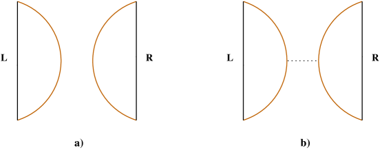
Figure 4: In the thermal AdS phase the left and right sides are classically disconnected. But there is a contribution from graviton exchange between them semiclassically which is responsible for the entanglement between the left and the right sides. This is depicted in b) where the dotted line represents the graviton exchange.

Hence according to the ER = EPR conjecture [11], the corresponding ER bridge connecting $B$ to $C$ should develop in the gravity description. However our solutions found in [5] do not show any signature of the development of ER bridge. This ER bridge ought to be nonclassical and cannot be seen in the classical gravity description. A similar behavior may be found in other examples. For instance consider the thermal AdS geometry that gives a dominant contribution to the partition function or the sum over geometries for $T<T_{HP}$, which is basically the Hawking-Page transition [19]. There are two thermal AdS geometries for the left and the right CFT’s separately. More precisely, as described in [8], two Lorentzian thermal AdS spaces are connected by a half of Euclidean thermal AdS solution in order to provide the initial state in (2.2). Thus this geometry is still dual to the thermofield double dynamics. It is clear that there is a nonvanishing L-R entanglement that is given by (2.8) once the temperature is nonzero. The corresponding entanglement entropy is of higher order in $G$ and hence cannot be seen in the classical gravity description. Indeed the two Lorentzian geometries of the left and the right sides are completely disconnected as depicted in Figure 4. Hence at the level of solution, the ER bridge does not appear, which is of course not a contradiction. There are many other examples of this type: The connected string solution in Figure  1c of [20] appears as two completely separate strings at the level of classical description.

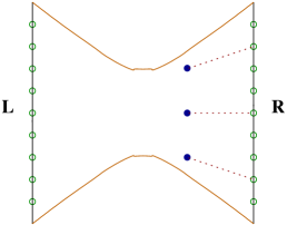
Figure 5: On the boundaries, the green dots represent the degrees of $C$ not covered by the classical gravity system. The rest represent the degrees in $B$ of the classical gravity including blue dots. The left-right entanglement is reduced to a non maximal one by the perturbations. The bulk degrees in $B$ (denoted by blue dots) is connected by the ER connecting $C$ (denoted by green dots) which is nonclassical. This effect is of order $1/N$ and cannot be seen in the classical gravity solutions.

Similarly in our example, the ER bridge is not seen at the level of classical description. The relevant degrees in $B$ fall gradually into the horizon that is responsible for the growth of the horizon area. Thus the entanglement is between these behind-horizon degrees and the corresponding degrees in $C$. The degrees in $C$ is not accessible from the classical gravity description. The connection is the quantum gravity fluctuation which is the semiclassical picture of the relevant ER bridge. We illustrate this in Figure 5.

Finally let us comment on the issue of the recurrence in the bulk. In the classical gravity description, the large $N$ limit is already taken, so there is basically no way to see this even in principle. But through the higher order effect in $1/N$ such as Hawking radiation, regaining of the transferred entanglement is allowed in principle, which can be a possible resolution of the black hole information paradox. But here we are dealing with an eternal black hole. Unlike the case of evaporating black hole in the flat space, the regaining time scale will be as large as $t_{rec}\sim e^{\alpha N^{2}}\sim e^{S_{grav}}$. At the final stage of recurrence, the entanglement between $B$ and $C$ is reduced and the system is back to the original state. In the time dependent perturbation of black hole in [5], this return actually happens when $t<0$, in which the entanglement between $B$ and $C$ is decreasing through interactions. Not that there is a failure of description at $t=\pm\infty$, which appears as the orbifold singularity in the three dimensional BTZ black hole. We view this as a simple failure of description, so in the bulk the recurrence will occur if one waits for long enough time.

References

- [1] J. M. Maldacena, “The Large N limit of superconformal field theories and supergravity,” Int. J. Theor. Phys. 38, 1113 (1999) [Adv. Theor. Math. Phys. 2, 231 (1998)] [hep-th/9711200].
- [2] S. S. Gubser, I. R. Klebanov and A. M. Polyakov, “Gauge theory correlators from noncritical string theory,” Phys. Lett. B 428, 105 (1998) [hep-th/9802109].
- [3] E. Witten, “Anti-de Sitter space and holography,” Adv. Theor. Math. Phys. 2, 253 (1998) [hep-th/9802150].
- [4] S. W. Hawking, “Breakdown of Predictability in Gravitational Collapse,” Phys. Rev. D 14, 2460 (1976). doi:10.1103/PhysRevD.14.2460
- [5] D. Bak, C. Kim, K. K. Kim and J. P. Song, “Holographic Micro Thermofield Geometries of BTZ Black Holes,” JHEP 1706, 079 (2017) [arXiv:1704.01030 [hep-th]].
- [6] M. Banados, C. Teitelboim and J. Zanelli, “The Black hole in three-dimensional space-time,” Phys. Rev. Lett. 69, 1849 (1992) [hep-th/9204099].
- [7] Y. Takahasi and H. Umezawa, “Thermo field dynamics,” Collect. Phenom. 2, 55 (1975).
- [8] J. M. Maldacena, “Eternal black holes in anti-de Sitter,” JHEP 0304, 021 (2003) [hep-th/0106112].
- [9] A. Einstein and N. Rosen, “The Particle Problem in the General Theory of Relativity,” Phys. Rev. 48, 73 (1935).
- [10] A. Einstein, B. Podolsky and N. Rosen, “Can quantum mechanical description of physical reality be considered complete?,” Phys. Rev. 47, 777 (1935).
- [11] J. Maldacena and L. Susskind, “Cool horizons for entangled black holes,” Fortsch. Phys. 61, 781 (2013) [arXiv:1306.0533 [hep-th]].
- [12] D. Bak, M. Gutperle and S. Hirano, “Three dimensional Janus and time-dependent black holes,” JHEP 0702, 068 (2007) [hep-th/0701108]; D. Bak, M. Gutperle and A. Karch, “Time dependent black holes and thermal equilibration,” JHEP 0712, 034 (2007) [arXiv:0708.3691 [hep-th]].
- [13] P. Gao, D. L. Jafferis and A. Wall, “Traversable Wormholes via a Double Trace Deformation,” arXiv:1608.05687 [hep-th].
- [14] E. Keski-Vakkuri, “Bulk and boundary dynamics in BTZ black holes,” Phys. Rev. D 59, 104001 (1999) [hep-th/9808037].
- [15] D. Bak and A. Trivella, “Quantum Information Metric on R X S(d-1),” JHEP 1709, 086 (2017) [arXiv:1707.05366 [hep-th]].
- [16] L. Dyson, M. Kleban and L. Susskind, “Disturbing implications of a cosmological constant,” JHEP 0210, 011 (2002) [hep-th/0208013].
- [17] L. Bombelli, R. K. Koul, J. Lee and R. D. Sorkin, “A Quantum Source of Entropy for Black Holes,” Phys. Rev. D 34, 373 (1986).
- [18] W. H. Zurek, “Decoherence, einselection, and the quantum origins of the classical,” Rev. Mod. Phys. 75, 715 (2003).
- [19] S. W. Hawking and D. N. Page, “Thermodynamics of Black Holes in anti-De Sitter Space,” Commun. Math. Phys. 87, 577 (1983).
- [20] D. Bak, A. Karch and L. G. Yaffe, “Debye screening in strongly coupled N=4 supersymmetric Yang-Mills plasma,” JHEP 0708, 049 (2007) [arXiv:0705.0994 [hep-th]].