Renormalization group flows and fixed points
for a scalar field in curved space with nonminimal $F(\phi)R$ coupling

Abstract

Using covariant methods, we construct and explore the Wetterich equation for a non-minimal coupling $F(\phi)R$ of a quantized scalar field to the Ricci scalar of a prescribed curved space. This includes the often considered non-minimal coupling $\xi\phi^{2}R$ as a special case. We consider the truncations without and with scale- and field-dependent wave function renormalization in dimensions between four and two. Thereby the main emphasis is on analytic and numerical solutions of the fixed point equations and the behavior in the vicinity of the corresponding fixed points. We determine the non-minimal coupling in the symmetric and spontaneously broken phases with vanishing and non-vanishing average fields, respectively. Using functional perturbative renormalization group methods, we discuss the leading universal contributions to the RG flow below the upper critical dimension $d=4$.

I Introduction

The renormalization group (RG) method is a flexible and powerful tool to study Quantum Field Theory in curved space-time. The traditional perturbative formulation was initiated in the papers nelspan82 ; buch84 ; Toms83 and is reviewed in book . Unfortunately, this formulation is essentially restricted to the Minimal Subtraction scheme of renormalization which hinders its applicability to infrared scales. Hence its applications to physical situations such as inflation or acceleration of the present-day universe require a great amount of phenomenological settings. This means that in many cases we are unable to derive the most relevant part of the quantum corrections, and therefore have to rely on general arguments based on covariance and dimension (see, e.g., PoImpo for a review).

The quantized scalar field coupled to gravity has always attracted a certain amount of interest. Recently this topic has again become interesting due to the role that gravitational effects might have on the Higgs decay, which could explain the stability of the Higgs potential at high energies (see, e.g., Higgs_decay for the latest situation and further references). Another important motivation is the growing interest on the effective potential of the Higgs field itself and its application to cosmology. Despite the limitations of the standard perturbative RG-methods in curved space-time, such a potential can be useful for consistently describing inflation Shaposh-08 ; BKS-2008 . In particular, it is known that the first- and second-loop corrections to the potential enable us to impose restrictions on the mass of the Higgs particle Shaposh-08 ; BKS-2008 . This means that the Higgs inflation, taking the opportune RG corrections into account, can provide falsifiable predictions for observational cosmology Tronconi:2017wps . The importance of the higher-loop corrections and the sensitivity of the results to infrared effects indicate that it may be worth employing a non-perturbative method of renormalization, especially to investigate the non-minimal coupling between the Higgs field and the scalar curvature.

Some well-known non-perturbative methods can be applied to curved space-time (see the reviews zinn ; Wipf ). Among these methods we include the functional renormalization group (FRG) approach FRG-review which has been much developed over the past decade, but has still been very little used to study quantum field theories in a curved background space. Exceptions are benedetti , in which the critical behavior of scalar field theories on spherical and hyperbolic spaces in the local potential approximation has been studied, and Fr , in which the symmetry restoration in de Sitter space has been investigated within the same approximation. Most papers adopting FRG methods to investigate the renormalization of matter fields in curved spaces considered scalar fields coupled to quantum gravitational fluctuations frg_diffeo ; Percacci-review ; Percacci-Vacca1 ; Narain:2009qa ; Narain:2009gb ; Zanusso:2009bs ; Vacca:2010mj to demonstrate that quantum gravity coupled to matter is a viable asymptotically safe theory with a non-trivial UV-fixed point as originally conjectured by S. Weinberg Weinberg-2d .

In the present paper we consider the functional RG method in a curved space-time and focus on a quantized scalar field $\phi$ coupled to a background with classical metric $g_{\mu\nu}$. As we are mainly interested in the matter sector, our attention will be mostly concentrated on the running of a non-minimal coupling function $F(\phi)$ which directly couples to the scalar-curvature through the interaction $F(\phi)R$. This truncation generalizes the more familiar scalar-curvature interaction $\xi\phi^{2}R$, which was previously explored with non-perturbative methods in AIP-EJPC . The generalization leading to $F(\phi)R$ and, in general, to non-polynomial self-interactions is interesting and was previously discussed in BKK in the framework of effective quantum field theory. The FRG approach offers a natural framework for dealing with such a truncation of the effective action.

It is well-known that in the conventional perturbative approach, the renormalization of a scalar theory with $\xi\phi^{2}R$ - interaction has the following properties:

• The presence of a term $\propto\xi\phi^{2}R$ is necessary for renormalizability of the theory. In particular, this means that the $\beta$-function for $\xi$ is non-zero, except at the fixed point. In one-loop order of perturbation theory the fixed point value is $\xi_{*}=1/6$ in four dimensions (see, e.g., book ). This value corresponds to the local conformal symmetry of the classical theory, and for the $d$-dimensional space the same symmetry requires $\xi_{*}=(d-2)/(4d-4)$. Let us note that the conformal fixed point is known only in four dimensions, because, for instance, in odd-dimensional spaces the one-loop beta-functions vanish and the results at two loops are not available. In the two-dimensional case $\xi_{*}=0$ is a fixed point.

• In all orders of the loop expansion the $\beta$-functions for the coupling constants of the theory (such as $\lambda$ in the $\lambda\phi^{4}$-interaction case) do not depend on $\xi$, while the $\beta$-function for $\xi$ is given by a polynomial expansion in these coupling constants corresponding to the expansion in loops. In the Minimal Subtraction scheme-based RG the $\beta$-function for $\xi$ is mass-independent. But a dependence on the mass is seen in the momentum-subtraction scheme of renormalization Bexi .

• The renormalization of the parameters of the vacuum action (depending on the background $g_{\mu\nu}$) depends on coupling constants and on $\xi$, while the inverse dependence is not seen.

In other words, in the loop expansion there is a hierarchy of the renormalization as follows:

$$\mbox{minimal terms}\ \ \to\ \ \mbox{non-minimal terms}\ \ \to\ \ \mbox{vacuum terms}.$$

Furthermore, beyond the one-loop order and in $4$ dimensions the $\beta$-function for $\xi$ is not proportional to the difference $\xi-1/6$. It is certainly interesting to see whether these features can be reproduced in a non-perturbative setting based on the FRG. In this work we employ the Wetterich equation, which probably is the most explored among all the currently known functional RG equations.

The paper is organized as follows. In Sect. II we formulate the FRG-equations for a scalar field theory with non-minimal interaction function $\,F(\phi)\,$ and briefly describe the method of calculations. Since the method is quite similar to the one which was explained in the previous work on $\,F(\phi)=\xi\phi^{2}$ AIP-EJPC , we need not present many details here. The section ends with the explicit form of the flow equation in any dimensions in the local potential approximation (LPA). In section III we study the solution of the fixed point equations and discuss the peculiarities in different dimensions. Thereby the main emphasis is on the fixed point equations for the non-minimal coupling. Analytical solutions in $2$ dimensions and numerical solutions in $d>2$ dimensions are presented and discussed in section IV. In the following section V the flow equations for the non-minimal coupling function with scale-dependent wave function renormalization $Z_{k}$ is derived. (the more complex equations with scale- and field-dependent wave function renormalization $Z_{k}(\phi)$ are given in appendix A). This latter improvement includes, in particular, the anomalous dimension of the field as the logarithmic scale derivative of $Z_{k}$ and goes under the name of improved LPA or LPA’. The results with $Z_{k}\neq 1$ are relevant in the spontaneously broken phase with non-vanishing expectation value of the scalar field. Finally, in section VI we study the perturbative RG in the vicinity of $4$ dimensions based on the truncation with scale and field dependent wave function renormalization. In leading order of the $\epsilon$-expansion we calculate the critical exponents for a scalar field coupled non-minimally to gravity. In section VII we draw our conclusions and discuss some perspectives for further work on the FRG in curved space.

II Scalar field in curved space with non-minimal coupling

The classical action of a single real scalar field in a curved space has the form

$$S=\int\sqrt{g}\,\left\{-\frac{1}{2}\phi\varDelta_{g}\phi+RF(\phi)+V(\phi)\right\}\,+\,S^{\mathrm{grav}}[g]\,.$$ (1)

Here and in what follows we assume Euclidean signature for the metric $g_{\mu\nu}$, denote the covariant Laplace operator with $\Delta_{g}$, and use the notation $\int\sqrt{g}=\int\mathrm{d}^{n}x\sqrt{g(x)}$. Our purpose is to explore the quantum effects of a scalar field, while the metric will be regarded as a classical external field. The classical action (1) involves a non-minimal term, which is known to be necessary for renormalizability in curved space. In the present paper we are mainly interested in the non-perturbative running of the non-minimal coupling function $F(\phi)$.

The ansatz for the scale dependent effective action is

$$\Gamma_{k} = \int\sqrt{g}\,\Big{\{}-\frac{1}{2}Z_{k}(\phi)\,\phi\varDelta_{g}\phi+RF_{k}(\phi)+V_{k}(\phi)\Big{\}}$$ (2)

$$+\Gamma_{k}^{\mathrm{grav}}[g]\,,$$

and it includes a scale dependent effective potential $V_{k}(\phi)$, a scale-dependent non-minimal coupling function $F_{k}(\phi)$ and a scale-dependent wave function renormalization $Z_{k}(\phi)$. Indeed, only in section VI and appendix A we do allow for a field-dependent $Z_{k}$, which in general has a rather lengthy flow equation. Therefore we will derive the flow equations first in the LPA’-approximation with scale-dependent but otherwise constant $Z_{k}$. The lengthy calculation for the case of a nonconstant wave-function renormalization is separated into appendix A.

Due to the above mentioned hierarchy of renormalization, we expect that the RG flow of the non-minimal function $F_{k}$ does not depend on the parameters in $\Gamma_{k}^{\mathrm{grav}}[g]$ and can be explored separately. Of course, the purely gravitational contribution, which is not considered in the present work, is of relevance for the intensively studied asymptotic safety scenario frg_diffeo ; Percacci-Vacca1 .

As invariant cutoff action we choose

$$\Delta S_{k} = \frac{1}{2}\int\sqrt{g}\,\phi R_{k}(-\varDelta_{g})\phi$$ (3)

$$\quad\hbox{{with}}\quad R_{k}(-\varDelta_{g})=Z_{k}r_{k}(-\varDelta_{g})\,.$$

$R_{k}$ must have the well-known properties of a cutoff function FRG-review and will be specified later (note that differently from the scalar curvature $R$, the cutoff-function $R_{k}$ is always shown with the subscript $k$). Next we introduce the anomalous dimension

$$\eta_{k}=-\frac{k\partial_{k}Z_{k}}{Z_{k}}=-\frac{\partial_{t}Z_{k}}{Z_{k}},\quad\hbox{{where}}\quad t=\log\frac{k}{\Lambda}\,.$$ (4)

The left hand side of the flow equation

$$\partial_{t}\Gamma_{k}[\phi]=\frac{1}{2}\,\mbox{tr}\,\left(\frac{\partial_{t}R_{k}}{\Gamma^{(2)}_{k}[\phi]+R_{k}}\right)$$ (5)

is simply given by

$$\partial_{t}\Gamma_{k} = \int\sqrt{g}\,\Big{\{}\frac{1}{2}\,\eta_{k}Z_{k}\,\phi\varDelta_{g}\phi+R\partial_{t}F_{k}(\phi)+\partial_{t}V_{k}(\phi)\Big{\}}$$ (6)

$$+\partial_{t}\Gamma_{k}^{\mathrm{grav}}[g].$$

In the flow equation we also need the second functional derivative of the effective action (2) with respect to the scalar field

$$\Gamma_{k}^{(2)}=-Z_{k}\varDelta_{g}+RF_{k}^{\prime\prime}(\phi)+V^{\prime\prime}_{k}(\phi)\,,$$ (7)

and the variation of the cutoff

$$\partial_{t}R_{k}=Z_{k}\left(\partial_{t}r_{k}-\eta_{k}r_{k}\right).$$ (8)

Thus for our truncation the r.h.s. of the flow equation takes the form

$$\frac{1}{2}\,\mbox{tr}\,\left(\frac{\partial_{t}R_{k}}{\Gamma^{(2)}_{k}[\phi]+R_{k}}\right)$$ (9)

$$\quad=\frac{1}{2}\,\mbox{tr}\,\Big{\{}\frac{Z_{k}(\partial_{t}-\eta_{k})r_{k}(-\varDelta_{g})}{-Z_{k}\varDelta_{g}+RF_{k}^{\prime\prime}(\phi)+V^{\prime\prime}_{k}(\phi)+Z_{k}r_{k}(-\varDelta_{g})}\Big{\}}\,.$$

To compare with the l.h.s. of the flow equation in (6) we expand this expression in powers of the scalar field and curvature. Therefore we set

$$V_{k}(\phi) = V_{k}(0)+\frac{V^{\prime\prime}_{k}(0)}{2}\phi^{2}+W_{k}(\phi)\,,$$

$$V^{\prime\prime}_{k}(\phi) = V_{k}^{\prime\prime}(0)+W^{\prime\prime}_{k}\,,$$ (10)

where $W_{k}(\phi)$ contains cubic and higher powers of the field. Then we arrive at the following form of the r.h.s.,

$$\frac{1}{2}\,\mbox{tr}\,\left(\frac{\partial_{t}R_{k}}{\Gamma^{(2)}_{k}[\phi]+R_{k}}\right)=\frac{1}{2}\,\mbox{tr}\,\frac{B_{k}(-\varDelta_{g})}{P_{k}(-\varDelta_{g})+\Sigma_{k}}\,,$$ (11)

where, following AIP-EJPC , we introduced the abbreviations

$$B_{k}(-\varDelta_{g}) =\partial_{t}r_{k}(-\varDelta_{g})-\eta_{k}r_{k}(-\varDelta_{g})\,,$$ (12)

$$P_{k}(-\varDelta_{g}) =-\varDelta_{g}+r_{k}(-\varDelta_{g})+\frac{V_{k}^{\prime\prime}(0)}{Z_{k}}\,,$$ (13)

$$\Sigma_{k}(\phi,R) =\frac{1}{Z_{k}}\big{[}RF^{\prime\prime}_{k}(\phi)+W^{\prime\prime}_{k}(\phi)\big{]}\,.$$ (14)

We will expand the r.h.s. on (11) in a power series in $\Sigma_{k}$ and thereby use $[B_{k},P_{k}]=0$. However, for a inhomogeneous field and curvature the spacetime-dependent $\Sigma_{k}$ does not commute with $B_{k}$ and $P_{k}$. But we still can write down the Neumann series

$$\,\mbox{tr}\,\Big{\{}\frac{B_{k}}{P_{k}+\Sigma_{k}}\Big{\}} = \sum_{m\geq 0}(-1)^{m}\,\,\mbox{tr}\,\Big{\{}Q_{k,1}\left(P_{k}^{-1}\,\Sigma_{k}\right)^{m}\Big{\}}\,,$$

$$Q_{k,m} = \frac{B_{k}}{P_{k}^{m}}.$$ (15)

To simplify the notations we skip the argument $-\varDelta_{g}$ of $B_{k},P_{k}$ and $Q_{k,m}$ as well as the arguments $\phi$ and $R$ of $\Sigma_{k}$.

The traces appearing in (15) can be computed via the heat kernel of the covariant Laplacian. The details of this procedure were described in off-diagonal ; AIP-EJPC and we just present the result for the optimized regulator function $r_{k}(s)=(k^{2}-s)\theta(k^{2}-s)$ Litim:2000ci . The expression for the trace in Eq. (15) is

$$Q_{k,m}(s) = \frac{2k^{2}-(k^{2}-s)\eta_{k}}{\Delta_{k}^{m}}\,\theta(k^{2}-s),$$

$$\Delta_{k} = k^{2}+\frac{m_{k}^{2}}{Z_{k}}\,.$$ (16)

Let us now consider the asymptotic small-$t$ expansion of $\exp(t\varDelta_{g})$,

$$\mathrm{e}^{t\varDelta_{g}}=\frac{1}{(4\pi t)^{d/2}}\left(A_{0}+tA_{1}+t^{2}A_{2}+\dots\right),$$ (17)

where the Schwinger-DeWitt coefficients have the well-known form,

$$A_{0}=1,\quad A_{1}=\frac{1}{6}R,\quad$$ (18)

$$A_{2}=\frac{1}{180}\Big{(}R_{\mu\nu\alpha\beta}R^{\mu\nu\alpha\beta}$$

$$\qquad\qquad\qquad-R_{\mu\nu}R^{\mu\nu}+6\varDelta_{g}R+\frac{5}{2}R^{2}\Big{)}.$$ (19)

With the help of the asymptotic expansion (17) the operators defined $Q_{k,m}$ in (15) (the reader may consult AIP-EJPC for more details), one arrives at the series expansions in position space,

$$\langle x|Q_{k,m}(-\varDelta_{g})|x\rangle=\frac{2}{(4\pi)^{d/2}}\frac{1}{\Delta_{k}^{m}}$$ (20)

$$\qquad\times\sum_{n\geq 0}\frac{k^{d-2n+2}}{\Gamma(d/2-n+1)}\left(1-\frac{\eta_{k}}{d-2n+2}\right)\,A_{n}(x)\,,$$

where $\Delta_{k}$ has been introduced in (16). Note that for even $d$ the series terminate since $1/\Gamma$ has zeros on the set of non-positive integers. At the same time our linear in curvature approximation is such that only the terms $\,n=0,1\,$ are relevant.

II.1 Local potential approximation

In a first step we consider the local potential approximation (LPA) with constant $\phi$ and constant scalar curvature $R$. Later we shall see how space-time dependent fields may modify the results. In the LPA no terms with derivatives of the field $\phi$ appear in the r.h.s. of the flow equation and hence $\partial_{t}Z_{k}$ vanishes in this approximation. The generalization to theories with Spontaneous Symmetry Breaking and non-trivial wave-function renormalization will be dealt with later on.

In the approximation considered $P_{k}$ commutes with $\Sigma_{k}$ and the Neumann series (15) simplify to

$$\,\mbox{tr}\,\left(\frac{B_{k}}{P_{k}+\Sigma_{k}}\right) = \sum_{m=0}^{\infty}(-1)^{m}\,\,\mbox{tr}\,Q_{k,1}P_{k}^{-m}\Sigma_{k}^{m}$$ (21)

$$= \sum_{m=0}^{\infty}(-1)^{m}\,\,\mbox{tr}\,Q_{k,m+1}\Sigma_{k}^{m}.$$

Inserting the expansion (20) with $\eta_{k}=0$ for the operators $Q_{k,m+1}$, one obtains a double sum over $m$ and $n$. The sum over $m$ can be carried out and provides as intermediate result

$$\frac{1}{2}\,\mbox{tr}\,\left(\frac{B_{k}}{P_{k}+\Sigma_{k}}\right)$$ (22)

$$\qquad=\frac{1}{(4\pi)^{d/2}}\sum_{n\geq 0}\frac{k^{d-2n+2}}{\Gamma(d/2-n+1)}\,\mbox{tr}\,\left(\frac{A_{n}}{\Delta_{k}+\Sigma_{k}}\right).$$

In the given truncation only the terms with $n=0$ and $1$ contribute, such that the relevant part of the r.h.s. of the flow equation is

$$\frac{1}{2}\,\mbox{tr}\,\left(\frac{B_{k}}{P_{k}+\Sigma_{k}}\right)$$

$$\quad=\mu_{d}\mathrm{Vol}\Big{(}\frac{k^{d+2}}{\Delta_{k}+\Sigma_{k}}+\frac{d}{12}\frac{k^{d}}{\Delta_{k}+\Sigma_{k}}\,R\Big{)}+\dots\,,$$ (23)

where Vol denotes the space-time volume. In addition we introduced the geometric factor

$$\mu_{d}=\frac{1}{(4\pi)^{d/2}\Gamma(\frac{d}{2}+1)},$$

$$\mbox{e.g.,}\quad\mu_{2}=\frac{1}{4\pi},\quad\mu_{3}=\frac{1}{6\pi^{2}},\quad\mu_{4}=\frac{1}{32\pi^{2}}\,.$$ (24)

Expanding $(\Delta_{k}+\Sigma_{k})^{-1}$ in Eq. (23) in powers of of the Ricci scalar, only the two leading terms contribute in our truncation, and we get

$$\frac{1}{2}\,\mbox{tr}\,\left(\frac{B_{k}}{P_{k}+\Sigma_{k}}\right)=k^{d}\mu_{d}\mathrm{Vol}\Bigg{[}k^{2}\,\Big{(}\frac{1}{k^{2}+V^{\prime\prime}_{k}}$$

$$\qquad\qquad-\frac{RF^{\prime\prime}_{k}}{(k^{2}+V^{\prime\prime}_{k})^{2}}\Big{)}+\frac{d}{12}\frac{R}{k^{2}+V^{\prime\prime}_{k}}\,\Bigg{]}+\dots\,.$$ (25)

Comparing with the l.h.s. of the Wetterich equation in (6) yields

$$\partial_{t}V_{k} =\mu_{d}k^{d}\frac{k^{2}}{k^{2}+V^{\prime\prime}_{k}}\,,$$ (26)

$$\partial_{t}F_{k} =\mu_{d}k^{d}\left(\frac{d}{12}\frac{1}{k^{2}+V^{\prime\prime}_{k}}-\frac{k^{2}F^{\prime\prime}_{k}}{(k^{2}+V^{\prime\prime}_{k})^{2}}\right)\,.$$ (27)

The first of these equations is exactly the same as in flat space-time, while the second one has no analogs in the flat-space limit. It is easy to see that these two flow equations imply that for even functions $V_{\Lambda}(\phi)$ and $F_{\Lambda}(\phi)$ at the UV-cutoff the scale dependent functions $V_{k}$ and $F_{k}$ stay even at all scales $k$.

Note that the flow of the effective potential $V_{k}(\phi)$ is independent of the non-minimal coupling function $F_{k}(\phi)$ and is exactly the same as in flat space-time. However it determines the running of the non-minimal coupling function $F_{k}(\phi)$.

III Fixed point solutions

To localize the fixed points of the RG flow we introduce the dimensionless field $\chi$, potential $v_{k}(\chi)$ and coupling function $f_{k}(\chi)$:

$$\phi=k^{(d-2)/2}\,\chi,\qquad V_{k}(\phi)=k^{d}\,v_{k}(\chi)\,,$$

$$\qquad\qquad F_{k}(\phi)=k^{d-2}f_{k}(\chi).$$ (28)

As a rule we denote dimensionful parameters and potentials by capital letters and the corresponding dimensionless quantities by small letters. The only exception is $\phi$ and $\chi$. By means of the identities

$$\partial_{\phi}^{2} = k^{2-d}\partial_{\chi}^{2}\,,$$

$$\partial_{t}V_{k} = k^{d}\left(\partial_{t}v_{k}+dv_{k}-\frac{d-2}{2}\,\chi\,\partial_{\chi}v_{k}\right)\,,$$ (29)

and similarly for $\partial_{t}F_{k}$, the flow equations for the dimensionless quantities take the form

$$\partial_{t}v_{k}+dv_{k}-\frac{d-2}{2}\chi v_{k}^{\prime}=\frac{\mu_{d}}{1+v^{\prime\prime}_{k}}\,,$$ (30)

$$\partial_{t}f_{k}+(d-2)f_{k}-\frac{d-2}{2}\,\chi f_{k}^{\prime}$$

$$\qquad\qquad\qquad\qquad=\frac{d}{12}\frac{\mu_{d}}{1+v^{\prime\prime}_{k}}-\frac{\mu_{d}f^{\prime\prime}_{k}}{(1+v^{\prime\prime}_{k})^{2}}\,.$$ (31)

Scaling solutions for the effective potential and the non-minimal coupling function are $k$-independent global solutions $v_{*}$ and $f_{*}$ of (30) which generalize the notion of a RG fixed point. We shall denote these fixed point solutions by a star in the following. The fixed point equations are

$$v^{\prime\prime}_{*} =\frac{2\mu_{d}}{2dv_{*}-(d-2)\chi v^{\prime}_{*}}-1\,,$$ (32)

$$f^{\prime\prime}_{*} =\frac{d}{12}(1+v_{*}^{\prime\prime})+\frac{d-2}{2\mu_{d}}(1+v_{*}^{\prime\prime})^{2}\left(\chi f_{*}^{\prime}-2f_{*}\right).$$ (33)

If the $v_{k}$ and $f_{k}$ are even functions at the cutoff, then they are even at any scale. Thus we assume the expansions

$$f_{*}(\chi) = f_{*}(0)+\frac{\xi_{*}}{2}\chi^{2}+\dots\,,$$

$$v_{*}(\chi) = v_{*}(0)+\frac{m_{*}^{2}}{2}\chi^{2}+\dots\,.$$ (34)

The constant term $f_{*}(0)$ relates to the dimensionless gravitational constant which feeds into the purely gravitational sector, which is not considered in the present work. Later we shall see that the fixed point value $\xi_{*}$ depends on this constant.

Inserting these expansions into the flow equation (31) (not the equation (33) where we solved for $f_{*}^{\prime\prime}$) with $\partial_{t}v_{*}=\partial_{t}f_{*}=0$ and comparing coefficients of $\chi^{0}$ relates $\xi_{*}\equiv f_{*}^{\prime\prime}(0)$ to $m_{*}$ and $f_{*}(0)$,

$$\xi_{*}=\frac{d}{12}(1+m_{*}^{2})-\frac{d-2}{\mu_{d}}(1+m_{*}^{2})^{2}\,f_{*}(0)\,.$$ (35)

Comparing coefficients of $\chi^{2}$ relates $\xi_{*}$ to the fourth derivatives of $v_{*}$ and $f_{*}$,

$$\left(\xi_{*}-\frac{d}{24}(1+m_{*}^{2})\right)v_{*}^{\prime\prime\prime\prime}(0)=\frac{1+m_{*}^{2}}{2}f_{*}^{\prime\prime\prime\prime}(0)\,.$$ (36)

For even functions $v_{*},f_{*}$ the fixed point equation (33) implies that $f^{\prime\prime\prime\prime}_{*}(0)$ is proportional to $v^{\prime\prime\prime\prime}_{*}(0)$. Using this relation in (36) gives rise to the simpler result (35).

III.1 Gaussian fixed points

In all dimensions there exist Gaussian fixed point solutions of (32) and (33) with constant scaling potential $v_{*}$. Then $m_{*}$ and $v_{*}^{\prime\prime\prime\prime}(0)$ both vanish and (36) does not yield information about $\xi_{*}$, but instead implies $f_{*}^{\prime\prime\prime\prime}(0)=0$. We conclude that at a Gaussian fixed point the non minimal function $f_{*}$ is a polynomial of degree $2$. The relation (32) determines the constant $v_{*}$ and (33) determines the coefficients of the quadratic polynomial $f_{*}$:

$$v_{*}(\chi)=\frac{\mu_{d}}{d},\qquad f_{*}(\chi)=\frac{\xi_{*}}{2}\chi^{2}+f_{*}(0),$$

$$\qquad\qquad\xi_{*}=\frac{d}{12}-\frac{d-2}{\mu_{d}}f_{*}(0)\,.$$ (37)

Only in two dimensions is the non-minimal parameter independent of the normalization $f_{*}(0)$. In higher dimensions $f_{*}(0)$ shifts the value of $\xi_{*}$

III.2 Non-Gaussian fixed points

Let us assume that there exists an interacting (non-Gaussian) fixed point with non-vanishing self-coupling $v_{*}^{\prime\prime\prime\prime}(0)$ and truncate the non-minimal function $f_{*}$ to an even polynomial of degree $2$ as in (37). Then $f_{*}^{\prime\prime\prime\prime}(0)=0$ and (36) determines $\xi_{*}$ which we insert into (35) to find $f_{*}(0)$:

$$\xi_{*}=\frac{d}{24}(1+m_{*}^{2}),$$ (38)

$$f_{*}(0)=\frac{d\mu_{d}}{24(d-2)(1+m_{*}^{2})}\,,\quad\hbox{{if}}\quad f_{*}^{\prime\prime\prime\prime}(0)=0,\;\;d>2\,.$$

Two dimensions are special since (35) yield for any fixed point – interacting or non-interacting – the simple relation

$$\xi_{*}=\frac{1}{6}(1+m_{*}^{2}),\qquad d=2,$$ (39)

independent of $f_{*}(0)$. Then (36) implies that at a non-Gaussian fixed point with non-vanishing $v_{*}^{\prime\prime\prime\prime}(0)$ the non-minimal function $f_{*}$ can not possibly be a polynomial of degree $2$.

In dimension higher than two a truncation with quadratic $f_{*}$ is inconsistent if $f_{*}(0)=0$. In other words $f_{*}(0)$ and $f_{*}^{\prime\prime\prime\prime}(0)$ cannot both vanish at a non-trivial fixed point. The truncation to a quadratic polynomial $f_{*}(\chi)$ has been discussed in detail for $d=4$ in AIP-EJPC . Let us now discuss the non-trivial fixed points which are expected to exist in $2\leq d<4$ dimensions in more detail. Actually for dimensions $3\leq d<4$ there exists one fixed point and below $3$ dimensions we expect a proliferation of fixed points with decreasing $d$.

4 dimensions:

If there would exist an interacting fixed point in $4$ dimensions (which probably is not the case) then we have for the truncation $f_{*}=f_{*}(0)+\xi_{*}\chi^{2}/2$ according to (38)

$$\xi_{*}=\frac{1}{6}(1+m^{2}_{*}),$$ (40)

which may deviate from the classical value $1/6$. This should be compared with the prediction of the standard Minimal Subtraction scheme-based one-loop RG for $\xi$, where a mass-dependence is not seen. Let us note that the mass-dependent $\beta$-functions are encountered in the physical (e.g., momentum-subtraction) renormalization schemes, including the non-minimal parameter $\xi$. In principle, starting from 3 loops the beta-function for $\xi$ is not proportional to $\xi-1/6$, as is known from Hathrell-82 .

3 dimensions:

The fixed point equation (32) takes the form

$$v^{\prime\prime}_{*}=\frac{1}{3\pi^{2}}\frac{1}{6v_{*}-\chi v_{*}^{\prime}}-1\,,$$ (41)

and admits a nontrivial scaling solution. Indeed, a numerical study reveals that only for the initial condition $v_{*}^{\prime\prime}(0)=m_{*}^{2}=-0.18605$ a non-trivial global solution of the (singular) differential equation exists Litim2 ; Wipf . As a result the critical $\xi_{*}$ in (38) is slightly smaller than the classical value $1/8$ (corresponding to the conformal coupling of a scalar field to gravity),

$$\xi_{*}=\frac{1}{8}(1+m^{2}_{*})=0.10174<\xi_{\mathrm{classical}}=0.125\,.$$ (42)

From $3$ to $4$ dimensions:

In four dimensions there is probably only the Gaussian fixed point solution for a scalar field wilsonfroehlich . In LPA it has constant potential

$$v_{*}\,=\frac{1}{128\pi^{2}}\quad\hbox{{and}}\quad\xi_{*}=\frac{1}{3}-64\pi^{2}f_{*}(0)\,.$$ (43)

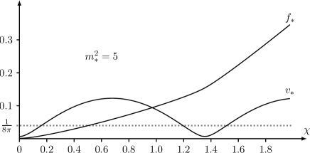
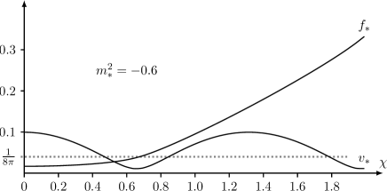
Let us see what happens when we approach the upper critical dimension $d=4$ from below. Since the FRG can be formulated in arbitrary space-time dimensions, we may continuously increase $d$ from $3$ to $4$ and study the limit of $\xi_{*}$ when $d\to 4$. In all dimensions $3\leq d<4$ there exists one non-trivial fixed point solution $v_{*}(\chi)$ with non-vanishing $v_{*}^{\prime\prime\prime\prime}(0)$ and $m_{*}^{2}<0$. Following codello2 ; Hellwig:2015woa we numerically solved the singular fixed point equation (32) for the dimensions given in Table 1 with the shooting method. An even solution depends only on its initial value $v_{*}(0)$ or equivalently on its initial curvature $v_{*}^{\prime\prime}(0)=m_{*}^{2}$. For a wrong initial condition $m_{*}^{2}$ the solution of the singular differential equation (32) becomes singular at a finite value $\chi_{\mathrm{max}}$ of the field. We fine-tuned the mass-parameter $m_{*}^{2}$ such that the solution extends to a maximal value of $\chi_{\mathrm{max}}$. If one continues with this fine-tuning then $\chi_{\mathrm{max}}$ finally increases until one (in principle) obtains a globally well-defined potential. After the global solutions $v_{*}$ is known one can proceed with solving the regular differential equation (33). The approximate fixed point values of $m_{*}^{2}$ and $\xi_{*}$ are listed in Table 1.

d	3	3.1	3.2	3.3	3.4	3.5	3.6
$m_{*}^{2}$	-0.18605	-0.15662	-0.13002	-0.10609	-0.08462	-0.06544	-0.04843
$\xi_{*}$	0.10174	0.10894	0.11600	0.12291	0.12968	0.13629	0.14274
d	3.7	3.8	3.9	3.95	3.98	3.99	3.999
$m_{*}^{2}$	-0.033457	-0.020430	-0.009283	-0.004406	-0.0017053	-0.0008430	-0.00008343
$\xi_{*}$	0.149009	0.155099	0.160992	0.163858	0.165551	0.166110	0.166611

Table 1: The curvature of the scaling potential with corresponding non-minimal parameter $\xi_{*}$ in various dimensions between $3$ and $4$. The results are plotted in Fig. 1.

For calculating the non-minimal coupling $\xi_{*}$ we used the relation (38) which applies to interacting fixed points in a truncation with quadratic $f_{*}$. These values are depicted in Figure 1, where we also plotted the classical conformal couplings and the interpolating polynomials of degree two for the calculated mass parameters and non-minimal parameters, given by

$$\begin{split}\xi_{*}(d)&=-0.0084105\,d^{2}+0.123892\,d-0.194295\,,\\ m_{*}^{2}(d)&=\hskip 11.38109pt-0.10973\,d^{2}+0.95288\,d\;-\;2.05629\,.\end{split}$$ (44)

In $4$ dimensions the interpolating polynomials yield the values $\xi_{*}=1.667$ and $m_{*}=-4\cdot 10^{-4}$. The value for $\xi_{*}$ agrees with the prediction (40) for an interacting fixed point with $m_{*}=0$ or with the prediction (43) for a Gaussian fixed point with $f^{-1}_{*}(0)=384\pi^{2}$.

Figure 1: The numerically determined values $m_{*}^{2}=v_{*}^{\prime\prime}(0)$ (marked by $\bullet$) with corresponding non-minimal parameters $\xi_{*}$ (marked by $\times$) in dimensions ranging from $3$ to $4$. The solid curve shows the classical conformal coupling. The dotted curves are fits by polynomials of degree $2$.

From the calculated values at $d=4-\epsilon$ with small $\epsilon\leq 0.3$ we extracted via an interpolation by a polynomial of degree $2$ the following $\epsilon$-expansions:

$$\xi_{*}(4-\epsilon) \approx 0.166669-0.055753\,\epsilon-0.010395\,\epsilon^{2}+\dots$$

$$\approx \;\frac{1}{6}-\frac{\epsilon}{18}-\frac{\epsilon^{2}}{96}+\dots\,,$$

$$m^{2}_{*}(4-\epsilon) \approx 3.2497\cdot 10^{-7}-0.083448\,\epsilon-0.093580\,\epsilon^{2}+\dots$$ (45)

$$\approx -\frac{\epsilon}{12}-\frac{468\epsilon^{2}}{5000}\,.$$

The $\epsilon$-expansion with scale and field-dependent wave function renormalization is reconsidered in section VI.

IV Exact and numerical solutions

Using the fixed point equation (32) for $v_{*}$, the differential equation (33) for $f_{*}$ can be written as

$$f_{*}^{\prime\prime}=\frac{2\mu_{d}}{2dv_{*}-(d-2)\chi v_{*}^{\prime}}\left[\frac{d}{12}+\frac{(d-2)(\chi f^{\prime}_{*}-2f_{*}}{2dv_{*}-(d-2)\chi v_{*}^{\prime}}\right].$$ (46)

This form is convenient for numerical studies.

IV.1 Analytic solutions in $2$ dimensions

In two dimensions there exist an infinite set of non-perturbative fixed points solutions of the fixed point equation morris

$$v^{\prime\prime}_{*}=\frac{1}{8\pi}\frac{1}{v_{*}}-1\,.$$ (47)

Multiplying with $v_{*}^{\prime}$ we immediately find a first integral. For an even scaling potential it reads

$$\frac{1}{2}v_{*}^{\prime\,2}(\chi)=\frac{1}{8\pi}\log\frac{v_{*}(\chi)}{v_{*}(0)}-\left(v_{*}(\chi)-v_{*}(0)\right)\,.$$ (48)

For a real potential the left hand side is non-negative which implies

$$\log\frac{v_{*}(\chi)}{v_{*}(0)}-8\pi\left(v_{*}(\chi)-v_{*}(0)\right)\geq 0\,.$$ (49)

By inspection one sees that for a positive initial value $v_{*}(0)$ the left hand side vanishes at two positive values $v_{*}(\chi)$ and is positive between these two nodes only. This means that for a positive $v_{*}(0)$ the potential $v_{*}(\chi)$ is bounded from below and from above. There are two possibilities morris ,

$$m_{*}^{2}>0 \Longrightarrow v_{*}(0)\leq v_{*}(\chi)\leq v_{*\mathrm{max}},$$

$$-1<m_{*}^{2}<0 \Longrightarrow v_{*\mathrm{min}}\leq v_{*}(\chi)\leq v_{*}(0)\,.$$ (50)

The fixed point equation (47) relates the potential and its curvature at the origin,

$$v_{*}(0)=\frac{1}{8\pi}\frac{1}{1+m_{*}^{2}}\,,$$ (51)

such that $v_{*}(0)$ varies between $0$ and $1/8\pi$ for the first class of solutions in (50) and is bigger than $1/8\pi$ for the second class. These bounded solutions show an oscillatory behavior. On the other hand, for a negative $v_{*}(0)$ the left hand side of (49) has only one node and $v_{*}(\chi)$ is negative for all $\chi$ and unbounded from below. This unstable solutions will be discarded on physical grounds.

The inverse function $\chi=\chi(v_{*})$ of a solution $v_{*}(\chi)$ of (47) is given by the integral codello2

$$\chi(v_{*})=\sqrt{4\pi}\int_{v_{*}(0)}^{v_{*}}\frac{\mathrm{d}u}{\sqrt{\log u/v_{*}(0)-8\pi(u-v_{*}(0))}}\,.$$ (52)

In $2$ dimensions the fixed point equation (33) for $f_{*}$ simplifies considerably and can easily be solved in terms of the scaling potential. Even solutions have the form

$$f_{*}(\chi)=\frac{\chi^{2}}{12}+\frac{v_{*}(\chi)}{6}+f_{*}(0),$$ (53)

with scaling potential given in (52). Each fixed point comes with its own periodic scaling potential $v_{*}$, non-minimal coupling function $f_{*}$ and positive non-minimal parameter,

$$\xi_{*}\equiv f_{*}^{\prime\prime}(0)=\frac{1}{6}(1+m^{2}_{*})=\frac{1}{48\pi\,v_{*}(0)}\in[0,\infty]\,.$$ (54)

The classical conformal coupling in two dimensions is $\xi_{*}=0$ and it is attained for $m_{*}^{2}=-1$. According to (50) this is the value for which the periodic scaling solutions with $m_{*}^{2}>-1$ cease to exist and one encounters the unstable scaling solutions with $m_{*}^{2}<-1$. Two typical solutions of the flow equation (47) with associated $f_{*}$ in (53) are depicted in Fig. 2. We normalized $f_{*}$ by setting $f_{*}(0)=0$. The potential $v_{*}$ in the upper figure has positive curvature $m_{*}^{2}$ at the origin and the one in the lower figure has negative $m_{*}^{2}$. Note that the asymptotic form of $f_{*}$ for large values of the field is independent of the scaling potential.

Figure 2: Two periodic scaling potentials $v_{*}(\chi)$ in two dimensions (without wave function renormalization) with corresponding coupling function $f_{*}$. We set $f_{*}(0)=0$ in (53).

Note that in $2$ dimensions we did not truncate $f_{*}(\chi)$ to a quadratic polynomial. Without wave function renormalization we observe a continuum of scaling potentials in two dimensions and correspondingly any value of $\xi_{*}$ between $0$ and $\infty$ seems to be possible. But we expect sizable corrections to the fixed point solutions if we include a wave function renormalization. With wave function renormalization one finds a discrete set of scaling potentials and correspondingly a discrete series of fixed point values $\xi_{*}$, see section V.

IV.2 Three and four dimensions

As discussed earlier, in three dimensions there is one non-trivial even scaling potential $v_{*}$ characterized by its (fine-tuned) mass-parameter. First we solved (41) for the scaling potential and in a second step obtained the fixed point coupling function $f_{*}$ from (46), which in $3$ dimensions reads

$$f^{\prime\prime}_{*}=\frac{1}{3\pi^{2}}\,\frac{1}{6v_{*}-\chi v^{\prime}_{*}}\left(\frac{1}{4}-\frac{2f_{*}-\chi f^{\prime}_{*}}{6v_{*}-\chi v^{\prime}_{*}}\right).$$ (55)

The numerical (even) solutions of the coupled system of differential equations (41,55) with initial condition $f_{*}(0)=0$ are depicted in Fig. 3.

Figure 3: The scaling potential $v_{*}(\chi)$ in three dimensions (without wave function renormalization) and the corresponding coupling function $f_{*}$ with initial condition $f_{*}(0)=0$.

According to (35) the non-minimal parameter $\xi_{*}$ depends on the unspecified fixed point value of the dimensionless gravitational constant $f_{*}(0)$

$$\xi_{*}=\frac{1}{4}\left(1+m_{*}^{2}\right)\left(1-24\pi^{2}\big{(}1+m_{*}^{2}\big{)}f_{*}(0)\right)\,,$$ (56)

and thus is not determined by $v_{*}$ alone.

In four dimensions the fixed point equation for $v_{*}$ admits only a constant solution belonging to the Gaussian fixed point. The corresponding even solution in (37) contains one free parameter,

$$f_{*}=\frac{\chi^{2}}{6}+f_{*}(0)\left(1-32\pi^{2}\chi^{2}\right)\,.$$ (57)

Thus at the Gaussian fixed point the solution $f_{*}$ is a sum of a constant and the quadratic term. The constant term $f_{*}(0)$ belongs to an induced Einstein-Hilbert term, and the quadratic term is required to provide perturbative renormalizability of the theory in curved space-time.

V Including the wave function renormalization $Z_{k}$

We have seen that there is no wave function renormalization in the truncation (2) if an even potential $V_{k}$ is expanded in powers of the field. But expanding in powers of the field may be inappropriate. For example, the potential at intermediate scales and the scaling solution need not be convex, contrary to the full effective potential $V_{k\to 0}$. Indeed, in most cases the scaling solution $v_{*}$ is non-convex. Since the flow is driven by fluctuations about the minimum $\phi_{0,k}$ of the effective potential it should be advantageous to expand both sides of the flow equation in powers of $\delta\phi_{k}=\phi-\phi_{0,k}$ rather than in powers of $\phi$. Since for an even classical potential one finds odd powers of $\delta\phi_{k}$ one should allow for odd powers in the flow equation. Then we expect a wave function renormalization already in the truncation (2). Actually it is well-known that without considering the anomalous dimension $\eta_{*}$ at the fixed point one misses interesting scaling solutions in two-dimensional systems in flat space-time delamotte .

For systems with running $Z_{k}$ (and therefore non-vanishing anomalous dimension) one easily reinstalls the $Z_{k}$ and $\eta_{k}$ dependence in the right hand side of the flow equations. Looking at the last expression in (9) we see that $V_{k}$ and $F_{k}$ must be divided by $Z_{k}$. Going back to (20) we conclude that the $n$’th term in (22) is multiplied with the factor $1-\eta_{k}/(d-2n+2)$. This way one obtains the flow equations with (field independent) wave function renormalization,

$$\partial_{t}V_{k} = \mu_{d}k^{d}\frac{k^{2}}{k^{2}+V^{\prime\prime}_{k}/Z_{k}}\left(1-\frac{\eta_{k}}{d+2}\right)\,,$$

$$\partial_{t}F_{k} = \mu_{d}k^{d}\Bigg{(}\frac{d}{12}\frac{1}{k^{2}+V^{\prime\prime}_{k}/Z_{k}}\left(1-\frac{\eta_{k}}{d}\right)$$ (58)

$$-\frac{k^{2}F^{\prime\prime}_{k}/Z_{k}}{(k^{2}+V^{\prime\prime}_{k}/Z_{k})^{2}}\left(1-\frac{\eta_{k}}{d+2}\right)\Bigg{)}\,.$$

For $Z_{k}=1$ and $\eta_{k}=0$ they simplify to the previously considered flow equation (26) and (27).

V.1 Scaling solutions

To study the fixed-point solutions we introduce the dimensionless “renormalized” field $\chi$ and functions $v_{k},f_{k}$ according to

$$\chi=k^{(2-d)/2}Z_{k}^{1/2}\,\phi,\qquad v_{k}(\chi)=k^{-d}\,V_{k}(\phi)$$

$$\qquad f_{k}(\chi)=k^{2-d}F_{k}(\phi)\,.$$ (59)

The flow equations for the dimensionless quantities take the form

$$\partial_{t}v_{k}+dv_{k}-\frac{d-2+\eta_{k}}{2}\,\chi v_{k}^{\prime}=\frac{\mu_{d}}{1+v^{\prime\prime}_{k}}\left(1-\frac{\eta_{k}}{d+2}\right)\,,$$

(60)

$$\partial_{t}f_{k}+(d-2)f_{k}-\frac{d-2+\eta_{k}}{2}\,\chi f_{k}^{\prime}$$

$$=\frac{d}{12}\frac{\mu_{d}}{1+v^{\prime\prime}_{k}}\left(1-\frac{\eta_{k}}{d}\right)-\frac{\mu_{d}f_{k}^{\prime\prime}}{(1+v^{\prime\prime}_{k})^{2}}\left(1-\frac{\eta_{k}}{d+2}\right).\,$$ (61)

For $\eta_{*}=0$ one recovers the flow equations (30) and (31) in the LPA. Compared to the flow equations without anomalous dimension the “effective space-time dimension” appearing in the geometric terms on the left hand side is $d+\eta_{k}$ instead of $d$. Note that it is the anomalous dimension $\eta_{k}$ – not the wave function renormalization $Z_{k}$ – that enters here as free parameter. It will be determined in a later stage when we find an algebraic equation which includes $\eta_{k}$.

The flow equations give rise to the fixed point equations within the LPA’:

$$dv_{*}-\frac{d-2+\eta_{*}}{2}\chi v^{\prime}_{*}=\frac{\mu_{d}}{1+v^{\prime\prime}_{*}}\left(1-\frac{\eta_{*}}{d+2}\right)\,,$$ (62)

$$(d-2)f_{*}-\frac{d-2+\eta_{*}}{2}\,\chi f_{*}^{\prime}$$

$$=\frac{d}{12}\frac{\mu_{d}}{1+v^{\prime\prime}_{*}}\left(1-\frac{\eta_{*}}{d}\right)-\frac{\mu_{d}f_{*}^{\prime\prime}}{(1+v^{\prime\prime}_{*})^{2}}\left(1-\frac{\eta_{*}}{d+2}\right).\,$$ (63)

The flow and fixed point equation for the potential in flat space has been studied extensively in the literature (see for example delamotte ; codello2 ) and hence we focus especially on the non-minimal coupling to gravity.

In passing we note that in $2$ dimension the differential equation (63) turns into a first order equation for $f_{*}^{\prime}$ which can be integrated. The solution with $f_{*}^{\prime}(0)=0$ has the form

$$f^{\prime}_{*}(x) =\frac{1}{3}\,\frac{2-\eta_{*}}{4-\eta_{*}}\;e^{Q(x)}\,\int_{0}^{x}dy\,e^{-Q(y)}\big{(}1+v^{\prime\prime}_{*}(y)\big{)},$$

$$Q(x) =\frac{8\pi\eta_{*}}{4-\eta_{*}}\int_{0}^{x}dy\,y\big{(}1+v_{*}^{\prime\prime}(y)\big{)}^{2}\,.$$ (64)

In the symmetric phase the non-minimal coupling is $\xi_{*}^{(s)}=f^{\prime\prime}_{*}(0)$. In the broken phase, where the field fluctuates about the minimum of the effective potential, it is more reasonable to characterize the coupling of the quantum field to space-time curvature by $f^{\prime\prime}_{k}($minimum of $v_{k})$. Thus below we consider the quantities

$$\xi_{*}^{(s)}=f^{\prime\prime}_{*}(0)\quad\hbox{{and}}\quad\xi_{*}^{(b)}=f_{*}^{\prime\prime}(\chi_{0*})\,,$$ (65)

defined at the origin and the minimum $\chi_{0*}$ of the fixed point potential $v_{*}$. Both are given by a generalization of (35)

$$\xi_{*}^{(s,b)} = \Bigg{(}\frac{d}{12}\left(1+v_{*}^{\prime\prime\,(s,b)}\right)\left(1-\frac{\eta_{*}}{d}\right)$$

$$-\frac{d-2}{\mu_{d}}\left(1+v_{*}^{\prime\prime\,(s,b)}\right)^{2}f_{*}^{(s,b)}\Bigg{)}\left(1-\frac{\eta_{*}}{d+2}\right)^{-1}\,,$$

where $v_{*}^{\prime\prime\,(s,b)}$ and $f_{*}^{(s,b)}$ in this equation denote $v_{*}^{\prime\prime}$ and $f_{*}$ at the origin and the minimum of $v_{*}$ respectively. Relation (V.1) yields a definite value only in two spacetime dimensions where it will be used below.

In higher dimensions the unknown initial values $f_{*}^{(s,b)}$ enter (V.1) and thus we seek a relation generalizing (36) which unambiguously fixed $\xi_{*}$. Comparing the second order terms in an expansion about the origin or minimum of (63) yields the relation

$$\left(\xi_{*}^{(s,b)}\Big{(}1-\frac{\eta_{*}}{d+2}\Big{)}-\frac{d}{24}\left(1+v_{*}^{\prime\prime\,(s,b)}\right)\Big{(}1-\frac{\eta_{*}}{d}\Big{)}\right)v_{*}^{\prime\prime\prime\prime\,(s,b)}=\frac{1+v_{*}^{\prime\prime(s,b)})}{2}\Big{(}1-\frac{\eta_{*}}{d+2}\Big{)}f_{*}^{\prime\prime\prime\prime\,(s,b)}-\frac{\eta_{*}\,\xi_{*}^{(s,b)}}{2\mu_{d}}\left(1+v_{*}^{\prime\prime\,(s,b)}\right)^{3},$$

(67)

with $v^{\prime\prime\prime\prime}_{*}$ and $f^{\prime\prime\prime\prime}_{*}$ evaluated at the origin or the minimum. Truncating $f_{*}$ to polynomials of degree two yields

$$\left(\xi_{*}^{(s,b)}\Big{(}1-\frac{\eta_{*}}{d+2}\Big{)}-\frac{d}{14}\left(1+v_{*}^{\prime\prime\,(s,b)}\right)\left(1-\frac{\eta_{*}}{d}\right)\right)v_{*}^{\prime\prime\prime\prime\,(s,b)}$$

$$\qquad\qquad=-\frac{\eta_{*}\,\xi_{*}^{(s,b)}}{2\mu_{d}}\left(1+v_{*}^{\prime\prime\,(s,b)}\right)^{3}\,,$$ (68)

which does not depend on an unspecified initial value for $f_{*}$. In numerical investigations it maybe advantageous to express the fourth derivative of $v_{*}$ at the origin or minimum by derivatives of lower order via the fixed point equation of $v_{*}$. To close the system of equations we need an equation for the anomalous dimension. This will be discussed next.

V.2 Flow equation for $Z_{k}$

To find an equation for the anomalous dimension one must admit an inhomogeneous field in the right hand side of the flow equation. We have argued earlier that in the given truncation and for an even potential a wave function renormalization only arises in a phase with broken symmetry. In the broken phase we set $\phi_{k}(x)=\phi_{0,k}+\delta\phi(x)$, where $\phi_{0,k}$ is a scale dependent minimum of the effective potential, i.e. $V^{\prime}_{k}(\phi_{0,k})=0$. Although a better choice would be to take the (in general inhomogeneous) minimum of $V_{k}(\phi)+F_{k}(\phi)R$, in the following we shall take the minimum of $V_{k}$ and this is justified for $\left|F_{k}R\right|\ll\left|V_{k}\right|$. The only term in the series (15) which produces a term proportional to $\delta\phi\varDelta_{g}\delta\phi$ is the one with $m=2$. The effect of the nonminimal term on the position of the minima can be taken into account perturbatively sponta , but this issue is beyond the scope of the present work. Since only the part $V^{\prime\prime}_{k}/Z_{k}$ of $\Sigma_{k}$ contributes to the running of $Z_{k}$ it is sufficient to consider the first term on the right hand side of

$$\frac{1}{2}\,\mbox{tr}\,\left(Q_{k,1}\Sigma_{k}\frac{1}{P_{k}}\Sigma_{k}\frac{1}{P_{k}}\right)$$

$$\qquad\qquad=\frac{1}{2Z_{k}^{2}}\,\mbox{tr}\,\left(Q_{k,2}V^{\prime\prime}_{k}\frac{1}{P_{k}}V^{\prime\prime}_{k}\right)+O(R)\,.$$ (69)

When we expand about the minimum of $V_{k}$ then $V_{k}^{\prime\prime}(0)$ in (13) is replaced by $V_{k}^{\prime\prime}(\phi_{0,k})$. To project the first term on the r.h.s. onto $\int\sqrt{g}\,\phi(-\varDelta_{g})\phi$ we note that its dependence on the spacetime geometry only enters via the covariant Laplacian in $Q_{k,2}$ and $P_{k}$. Thus we may take the result in flat space time ballhausen ; FRG-review ; Wipf and just replace the Laplacian by the covariant Laplacian, in accordance to what has been explained also in the Introduction. With

$$V_{k}^{\prime\prime}(\phi_{k})\,=\,V_{k}^{\prime\prime}(\phi_{0,k})+V^{\prime\prime\prime}_{k}(\phi_{0,k})\delta\phi\,+\,\dots$$ (70)

one obtains

$$\frac{V_{k}^{\prime\prime\prime 2}(\phi_{0,k})}{Z_{k}^{2}}\,\mbox{tr}\,\left(Q_{k,2}\delta\phi\frac{1}{P_{k}}\delta\phi\right)$$ (71)

$$\qquad=\mu_{d}k^{d+2}\frac{V_{k}^{\prime\prime\prime\,2}(\phi_{0,k})/Z_{k}^{2}}{(k^{2}+V^{\prime\prime}_{k}(\phi_{0,k})/Z_{k})^{4}}\int\sqrt{g}\,\delta\phi\varDelta_{g}\delta\phi+\dots\,,$$

where the dotted terms do not contribute to the running of $Z_{k}$. Comparing with (4) finally yields

$$\eta_{k}\equiv-\frac{\partial_{t}Z_{k}}{Z_{k}}=\mu_{d}k^{d+2}\frac{V_{k}^{\prime\prime\prime\,2}(\phi_{0,k})/Z_{k}^{3}}{(k^{2}+V^{\prime\prime}_{k}(\phi_{0,k})/Z_{k})^{4}}\,.$$ (72)

In terms of the dimensionless quantities in (59) this equation reads

$$\eta_{k}=\mu_{d}\frac{v_{k}^{\prime\prime\prime\,2}(\chi_{0,k})}{(1+v^{\prime\prime}_{k}(\chi_{0,k}))^{4}}\,,$$ (73)

such that

$$\eta_{*}=\mu_{d}\frac{v_{*}^{\prime\prime\prime\,2}(\chi_{0*})}{\big{(}1+v^{\prime\prime}_{*}(\chi_{0*})\big{)}^{4}}\,,$$ (74)

and it has been studied in detail in codello2 ; Hellwig:2015woa . The last expression yields the anomalous dimension at criticality which enters the expression (67) and (68) for the non-minimal couplings to the Ricci scalar.

V.3 Numerical evaluation of $\xi_{*}$ in LPA’

In our numerical studies we followed codello2 ; Hellwig:2015woa and first solved the fixed point equation (62) for $v_{*}$ with an educated first guess for $\eta_{*}$. With the shooting method we determined for this $\eta_{*}$ the (approximate) value of $m_{*}^{2}$ for which the differential equation admits a global solution. From the global solution we extracted the corresponding value of $\eta_{*}$ according to (68). Then we used this value as improved guess for the shooting method. This process is repeated until the values of $\eta_{*}$ converge and one obtains a self-consistent solution of the flow equation and the equation determining $\eta_{*}$. Then one calculates the value of $\xi_{*}$ from this self-consistent solution.

Two dimensions:

We analyze the fixed point corresponding to the critical Ising model coupled non-minimally to gravity. From the known values of $\eta_{*}$ and $v^{\prime\prime}(0)$ in the Ising and Tri-Ising class Hellwig:2015woa we calculated $v^{\prime\prime}(\chi_{0*})$ and the corresponding values $\xi_{*}$ from (V.1):

$$\xi_{*}^{(s)} = \frac{1}{6}(1+v_{*}^{\prime\prime}\big{(}0)\big{)}\frac{1-\eta_{*}/2}{1-\eta_{*}/4}\,,$$

$$\xi_{*}^{(b)} = \frac{1}{6}(1+v_{*}^{\prime\prime}\big{(}\chi_{0*})\big{)}\frac{1-\eta_{*}/2}{1-\eta_{*}/4}\,.$$ (75)

The results for the Ising and Tri-Ising classes are listed in Table 2.

¡ universality class	$\eta_{*}$	$v_{*}^{\prime\prime}(0)$	$v_{*}^{\prime\prime}(\chi_{0*})$	$\xi_{*}^{(s)}$	$\xi_{*}^{(b)}$	$\xi_{\text{class}}$
$d=2$ Ising class LPA’	$0.4364$	$-0.3583$	$1.2489$	$0.0939$	$0.0182$	$0.0000$
$d=2$ Tri-Ising class LPA’	$0.3119$	$+0.2597$	$0.7534$	$0.1922$	$0.0078$	$0.0000$
$d=3$ Wilson-Fisher LPA	$0.0000$	$-0.1859$	$0.4571$	$0.1018$	$0.1821$	$0.1250$
$d=3$ Wilson-Fisher LPA’	$0.1120$	$-0.1356$	$0.3093$	$0.0895$	$0.1302$	$0.1250$

Table 2: The anomalous dimensions, second derivative of the fixed point potentials at the origin and the minimum and the non-minimal couplings at criticality defined at the origin and at minimum of the scaling potential. The last column contains the classical conformal couplings.

Three dimensions:

Here we assume the truncation in which $f_{*}(\chi)$ is a polynomial of degree $2$, such that we may use (68) to calculate $\xi_{*}$ for fluctuations about the origin and about $\chi_{0*}$. With the known values $\eta_{*}$ and $v^{\prime\prime}(0)$ from Hellwig:2015woa we solved the fixed point equations numerically and extracted $v^{\prime\prime}(\chi_{0*})$ and $v^{\prime\prime\prime\prime}_{*}(\chi_{0*})$. These then yield the values of the minimal couplings given in Table 2. In the same Table we also included the corresponding values for $\xi_{*}$ calculated in the LPA approximation with $\eta_{*}=0$. In three dimensions the classical conformal coupling $\xi_{\mathrm{class}}=0.125$ lies between the values extracted for fluctuations about the origin and about the minimum of the scaling potential. This holds true in the LPA and in the LPA’ approximations.

VI Universality and perturbation theory in $d=4-\epsilon$

In this section we concentrate on the scheme-independent (universal) contribution to the flow of (2) with field dependent potential $V_{k}(\phi)$, non-minimal coupling $F_{k}(\phi)$ and wave function renormalization $Z_{k}(\phi)$. These contributions correspond to the RG flow induced by the subtraction of the $1/\epsilon$ poles of dimensional regularization ($\overline{\rm MS}$ scheme) below the upper critical dimension $d=4$ of a $\phi^{4}$ model which is non-minimally coupled to a curved geometry.

We study the leading universal contributions in the $\epsilon$-expansion using the approach introduced by O’Dwyer and Osborn in ODwyer:2007brp which was later further refined and named functional perturbative RG in Codello:2017hhh . The functional perturbative flow is fully equivalent to the flow induced by standard coupling’s perturbation theory with minimal subtraction in the $\epsilon$-expansion. In fact, all perturbative beta functionals can be derived by means of standard renormalization of the same Feynman diagrams which in the standard approach renormalize the coupling and generate anomalous operators’ scaling dimensions.

In the present work we find it more instructive to detect which contributions are universal by extracting the logarithmic scaling terms of the non-perturbative flow of the full system $V_{k}(\phi)$, $F_{k}(\phi)$ and $Z_{k}(\phi)$. A complete representation of the flow of this system for arbitrary cutoff can be found in appendix A. In the same appendix we also briefly explain which techniques are used to extract the universal contributions and further elaborate on other universality classes coupled to a curved geometry.

The leading universal part that is extracted from the non-perturbative RG flow in $d=4$ at the second order of the derivative expansion given in appendix A is

$$\begin{split}\partial_{t}V_{k}&=\frac{1}{(4\pi)^{2}}\frac{(V_{k}^{\prime\prime})^{2}}{2Z^{2}_{k}}\,,\quad\partial_{t}F_{k}=-\frac{1}{(4\pi)^{2}}\frac{V_{k}^{\prime\prime}}{Z_{k}}\left(\frac{1}{6}-\frac{F_{k}^{\prime\prime}}{Z_{k}}\right)\,,\\ \partial_{t}Z_{k}&=\frac{1}{(4\pi)^{2}}\frac{1}{Z^{2}_{k}}\left(Z_{k}^{\prime\prime}V_{k}^{\prime\prime}+Z_{k}^{\prime}V_{k}^{\prime\prime\prime}\right)\,.\end{split}$$ (76)

In the limit of small deformations of $Z_{k}(\phi)$ around $Z_{k}(\phi)=1$, this flow can be checked against the flat-space case obtained in ODwyer:2007brp ; Codello:2017hhh . Specifically, the flow of $V_{k}(\phi)$ entails the one-loop leading renormalization of the $\phi^{4}$ or Ising’s universality class. Furthermore, the flow of the wave function can also be checked against the results of the derivative expansion, which also appear in ODwyer:2007brp ; Codello:2017hhh .

Let us denote the constant part of the wavefunction as $Z_{k,0}=Z_{k}(0)$, which we now decorate with an additional label to distinguish it from the full field-dependent $Z_{k}=Z_{k}(\phi)$. As in Eq. (59) we define the dimensionless field $\phi=k^{d/2-1}Z_{k,0}^{-1/2}\chi$, the dimensionless functions $v_{k}$ and $f_{k}$ and, in addition, the dimensionless wave function renormalization

$$z_{k}(\chi)=Z_{k,0}^{-1}Z_{k}(\phi)$$ (77)

in $d=4-\epsilon$. The rescaling of $Z_{k}(\phi)$ ensures the boundary condition $z_{k}(0)=1$. The perturbative RG flow of these functions is

$$\partial_{t}v_{k} = -4v_{k}+\chi v_{k}^{\prime}+\epsilon\left(v_{k}-\frac{1}{2}\chi v_{k}^{\prime}\right)$$

$$+\frac{1}{2}\eta_{k}\chi v_{k}^{\prime}+\frac{1}{(4\pi)^{2}}\frac{1}{2}\frac{(v_{k}^{\prime\prime})^{2}}{z^{2}_{k}}\,,$$

$$\partial_{t}f_{k} = -2f_{k}+\chi f^{\prime}_{k}+\epsilon\left(f_{k}-\frac{1}{2}\chi f^{\prime}_{k}\right)$$

$$+\frac{1}{2}\eta_{k}\chi f^{\prime}_{k}-\frac{1}{(4\pi)^{2}}\frac{v_{k}^{\prime\prime}}{z_{k}}\left(\frac{1}{6}-\frac{f_{k}^{\prime\prime}}{z_{k}}\right)\,,$$

$$\partial_{t}z_{k} = \eta_{k}z_{k}+\chi z^{\prime}_{k}-\frac{\epsilon}{2}\chi z_{k}^{\prime}+\frac{1}{2}\eta_{k}\chi z_{k}^{\prime}$$ (78)

$$+\frac{1}{(4\pi)^{2}}\frac{1}{z_{k}^{2}}\left(z_{k}^{\prime\prime}v_{k}^{\prime\prime}+z_{k}^{\prime}v_{k}^{\prime\prime\prime}\right)\,.$$

The anomalous dimension $\eta_{k}$ can be determined enforcing the boundary condition $z_{k}(0)=1$, but it is nonzero only at two-loops ODwyer:2007brp ; Codello:2017hhh , thus it yields a correction of order $\epsilon^{2}$, as expected from standard perturbation theory. Since our results are limited to the leading order of the $\epsilon$-expansion, we shall neglect it for the remainder of this section.

The perturbative setting simplifies the study of $k$-independent solutions of (78) considerably. As expected, we find two interesting fixed points: The non-trivial fixed point is

$$v_{*}(\chi)=\frac{1}{(4\pi)^{2}}\,\frac{\epsilon}{3}\,\frac{\chi^{4}}{4!}\,,\quad f_{*}(\chi)=\frac{1}{6}\frac{\chi^{2}}{2!}\,,\quad z_{*}(\chi)=1\,,$$ (79)

while the generalization of the Gaussian fixed point

$$v_{*}(\chi)=0\,,\quad f_{*}(\chi)=\frac{1}{6}\frac{\chi^{2}}{2!}\,,\quad z_{*}(\chi)=1\,.$$ (80)

In both cases the non-minimal coupling $\xi$ takes the expected value $1/6$ in $d=4$. It is interesting that the nontrivial fixed point does not exhibit the expected analytic continuation of the formula $\xi=(d-2)/(4d-4)=1/6-\epsilon/36$ in $d=4-\epsilon$, which makes it more difficult to interpret it as the perturbative analog of (45). Written in this form, this result is scheme independent and therefore fully independent of any cutoff choice that was made throughout the rest of this paper, thus intuitively we could think of (40) as barring some explicit cutoff dependence which is ignored by the perturbative analysis.

The scaling analysis of (78) around the nontrivial fixed point (79) is also very simple. In $d=4-\epsilon$, for arbitrarily small $\epsilon$, the mixing of the operators is selected by the mass dimension. More precisely, we can parametrize an arbitrary deformation of the fixed point solution as

$$v_{k}(\chi)=v_{*}(\chi)+\frac{\lambda_{n}}{n!}\chi^{n}\,,\qquad z_{k}(\chi)=1+\frac{\zeta_{n-4}}{(n-4)!}\chi^{n-4}\,,$$

$$\qquad\qquad f_{k}(\chi)=f_{*}(\chi)+\frac{\xi_{n-2}}{(n-2)!}\chi^{n-2}\,,$$ (81)

for a given natural number $n$. The implicit condition is that only polynomial interactions are allowed $\lambda_{m}=\xi_{m}=\zeta_{m}=0$ if $m$ is a negative number Bridle:2016nsu . This implies, for example, that the first two monomials of $v_{k}$ cannot mix, and that the first nontrivial mixing occurs between $\phi^{2}$ and $R$. This pattern continues up to the point in which all functions are mixed together starting with the (almost) marginal operators $\phi^{4}$, $\phi^{2}R$ and $(\partial\phi)^{2}$. The stability matrix in the basis $\left(\lambda_{n},\xi_{n-2},\zeta_{n-4}\right)$ must be diagonalized at the fixed point (79). The negative of the eigenvalues of the stability matrix are the spectrum of scaling (critical) exponents $\theta_{n,i}$ of the theory. We label three sets of eigenvalues

$$\begin{split}&\theta_{n,1}=4-n-\frac{1}{6}\left(6-4n+n^{2}\right)\epsilon\qquad{\rm for}\quad n\geq 0\,,\\ &\theta_{n,2}=4-n-\frac{1}{6}\left(18-8n+n^{2}\right)\epsilon\hskip 17.07164pt{\rm for}\quad n\geq 2\,,\\ &\theta_{n,3}=-\frac{1}{6}\left(n-4\right)\left(6+(n-6)\epsilon\right)\qquad{\rm for}\quad n\geq 4\,.\end{split}$$ (82)

For almost all values of $n$ the degeneracy of the critical exponents is lifted and, following the standard arguments of perturbation theory, we could interpret the operators corresponding to the above three sets as (normal ordered) generalizations of $\phi^{n}$, $\phi^{n-1}R$ and $\phi^{n-4}(\partial\phi)^{2}$ respectively. In the flat-space limit, these results agree with those on the renormalization of the composite operators of the form $\phi^{n}$, which are known by several means (see for example ODwyer:2007brp and references therein).

One can also see that the use of the invariance under reparametrizations of the wavefuction has the effect that there is exactly one marginal operator $\theta_{4,3}=0$, roughly corresponding to the kinetic term Osborn:2011kw . The eigenvalues of the stability matrix reveal some mixing among the considered operators. For $n\geq 6$ the operators $\phi^{n}$, $\phi^{n-1}R$ and $\phi^{n-4}(\partial\phi)^{2}$ begin mixing with higher derivative operators. This includes in particular those with four derivatives as discussed in Codello:2017hhh . We recommend Pagani:2016pad ; Pagani:2017tdr for more details on the renormalization of composite operators in the functional approach and Pagani:2016dof for very non-trivial applications of those results.

VII Summary and Conclusions

We have discussed and explored functional renormalization group (FRG) equations for the non-minimal coupling $F(\phi)R$ of a quantized scalar field to a classical background geometry with Ricci scalar $R$. We showed that – similarly as in standard perturbation theory – the couplings in the matter sector enter the flow equation for the scale dependent non-minimal coupling function $F_{k}(\phi)$ but not vice-versa. The flow of the effective potential and field-dependent wave function renormalization are independent of $F_{k}$. In all truncations and dimensions considered the function $F_{k}$ fulfills an inhomogeneous linear differential equation with coefficient functions depending on the scale dependent effective potential $V_{k}$. It is remarkable that the $\beta$-function for the dimensionless non-minimal coupling function $f_{k}$ and the corresponding non-minimal coupling $\xi_{k}=f_{k}^{\prime\prime}(0)$ is reproducing further important features of the standard perturbative RG, which can be observed beyond one-loop order. In particular, the FRG-based $\beta$-function in $d$ dimensions

$$\begin{split}\beta(\xi)=\partial_{t}\xi_{k}&=2\mu_{d}\frac{v^{\prime\prime\prime\prime}_{k}(0)}{(1+m_{k}^{2})^{3}}\left(\xi_{k}\left(1-\frac{\eta_{k}}{d+2}\right)-(1+m_{k}^{2})\frac{d+\eta_{k}}{24}\right)-\mu_{d}\frac{f_{k}^{\prime\prime\prime\prime}(0)}{(1+m_{k}^{2})^{2}}\left(1-\frac{\eta_{k}}{d+2}\right),\\ \quad\hbox{{with}}\quad m_{k}^{2}=v_{k}^{\prime\prime}(0)\,,\end{split}$$ (83)

following from the flow equation (54) in LPA’, does not necessarily lead to a conformal fixed point at $\xi_{*}=1/6$ in four dimensions, as predicted by one-loop perturbation theory book . In addition, at a Gaussian fixed point with vanishing $v_{*}^{\prime\prime\prime\prime}(0)$ we necessarily have $f_{*}^{\prime\prime\prime\prime}(0)=0$. In LPA’ and the symmetric phase we do not observe a renormalization of the wave function. This mirrors the same property in flat spacetime. On the other hand, in the broken phase a non-zero wave function renormalization changes the fixed point solutions for the non-minimal coupling function $f_{*}$ and the corresponding non-minimal coupling $\xi_{*}$, exactly as we have described in the introduction on general grounds. Finally, Eq. 84 show the IR decoupling, that was described in the momentum-subtraction scheme of renormalization in curved space BuGui .

In two dimensions the equations and solutions simplify considerably. Both in LPA and LPA’ we could solve the fixed point equation for $f_{*}$ analytically in terms of the fixed point potential $v_{*}$. In both truncations there is an unambiguous prediction for the non-minimal coupling, given in (54) and (75), respectively. In LPA’ one recovers all minimal models in the Landau classification of two-dimensional conformal field theories. From numerical solutions of the flow equation for $v_{*}$ with self-consistently determined anomalous dimensions one can extract the non-minimal couplings $\xi_{*}$ at criticality for this class of model. We presented the results in the symmetric and broken phases both for the Ising and tri-Ising class.

For a sequence of dimensions between dimensions $3$ and $4$ we determined $\xi_{*}$ for the non-Gaussian fixed points. From an interpolation of the corresponding values as a function of the dimension $d=4-\epsilon$ we could numerically extract the $\epsilon$-expansion of $\xi_{*}(\epsilon)$ in LPA. The same has been achieved in the framework of the so-called functional perturbative RG, applied to non-minimally coupled scalars in $d=4-\epsilon$ dimensions with field and scale dependent wave function renormalization. Besides the flow of the fixed point potential and wave function renormalization we calculated the flow of the non-minimal coupling function in order $\epsilon$ from the FRG. The contribution of order $\epsilon$ to the non-minimal coupling – calculated numerically in LPA and analytically in the functional perturbative RG – are different. Future numerical efforts with a less crude truncation may improve the situation. A first step would be to recalculate the values in Table 1 in a truncation with wave-function renormalization and self-consistently determined $\eta_{*}$.

In LPA’ the non-minimal coupling function $f_{k}$ obeys a non-singular linear inhomogeneous differential equation. Thus parity-even fixed point solutions depend only on one initial condition, say $f_{*}(0)$, which is not quantized. For $d\neq 2$ this free parameter enters the equation for $\xi_{*}$ and this ambiguity is apparently fixed by a suitable polynomial truncation of $f_{*}$. It maybe interesting to see how the inclusion of the purely gravitational contribution $\Gamma_{k}^{\text{grav}}[g]$ could lift this degeneracy.

We have also discussed the universal contributions to the flow of the system which appear as the logarithmically scaling terms of the renormalization group flow and which are in one-to-one correspondence with the renormalization induced by subtracting $1/\epsilon$ poles of dimensional regularization. These contributions offer a different perspective on the results in $d=4-\epsilon$ and specifically on their interpolation from the four dimensional limit in terms of universal contributions. The universal results show the role that the cutoff has in estimating the critical coupling $\xi$ and the critical properties in dimensions lower than four. While a dependence on the cutoff function is a generally unwanted feature, it is also true that only with the Wetterich equation and the scaling solutions’ approach one can obtain a realistic numerical estimation of the critical exponents of the scalar theory in a dimensionality that is genuinely lower than four.

A natural extension of the present work would be to determine the running of $F_{k}$ in a non-minimal term of the form

$$\int\sqrt{g}\,F_{k}(\phi,R)$$ (84)

in the scale dependent effective action. Such a term has been investigated in Narain:2009qa with the inclusion of metric fluctuations and the emphasis on the asymptotic safety scenario. It is generated during the FRG-flow from the ultraviolet to the infrared and has been considered in studies of Higgs inflation (see, for example, defelice ). More demanding and maybe even more interesting would be the calculation of the dominant non-local contributions to $\Gamma_{k}^{\mathrm{grav}}$ within the FRG-approach Codello:2015oqa ; Rachwal:2016vte .

Appendix A Field-dependent wave function renormalization

In this appendix we present the integral form of the non-perturbative RG flow of the effective action that includes a field dependent wave function renormalization $Z_{k}(\phi)$ as in (2). The field dependence in the coefficient of the kinetic term makes the flow considerably more complex, which is why we provide it in the form of a momentum space integral and only discuss some of its features with more detail.

There are two main strategies to compute the flow of the functions $V_{k}(\phi)$, $F_{k}(\phi)$ and $Z_{k}(\phi)$. On the one hand, one can use the heat kernel of the Laplacian operator $\Delta_{g}$ to give a computable representation of the functional trace (5) as it is done in section II of the main text. On the other hand, one can obtain the same RG flows by applying a vertex expansion to (5). In the latter case, the flows of $V_{k}(\phi)$, $F_{k}(\phi)$, and $Z_{k}(\phi)$ are seen respectively from the zero-point function, the two-point function of the scalar field, and the one-point function of $h_{\mu\nu}$, where $h_{\mu\nu}$ is a small deformation of the metric around a flat Euclidean background $g_{\mu\nu}=\delta_{\mu\nu}+h_{\mu\nu}$. In this appendix we shall present the results derived with the vertex expansion methods described in Codello:2013wxa . It is a rather non-trivial check that they coincide with those coming from the heat kernel which we derive and use in the main text, especially in the case of the one-point function of $h_{\mu\nu}$.

In order to condense the notation, let us first define a modified field dependent propagator

$${\cal G}_{k}\equiv{\cal G}_{k}(q^{2};\phi)=\left(Z_{k}(\phi)q^{2}+V_{k}^{\prime\prime}(\phi)+R_{k}(q^{2})\right)^{-1}\,,$$ (85)

which is evaluated in momentum space and at a constant field configuration $\phi$. The modified propagator differs from the standard propagator of the field by the presence of the cutoff kernel $R_{k}(\Delta_{g})$, which in flat space becomes a simple function of the momentum square $q^{2}$ in agreement with its covariant form (3). Let us also use primes to denote the first and second derivatives of ${\cal G}_{k}$ with respect to the momentum square argument

$${\cal G}_{k}^{\prime}=\partial_{q^{2}}{\cal G}_{k}(q^{2};\phi)\,,\qquad{\cal G}_{k}^{\prime\prime}=\partial^{2}_{q^{2}}{\cal G}_{k}(q^{2};\phi)\,.$$ (86)

Ideally, the cutoff kernel is assumed to be at least twice differentiable, but meaningful formulas can be found for optimized cutoffs such as (16) used in the main text. For a generic cutoff function, we find the following integral representations of the flows

$$\begin{split}\partial_{t}V_{k}&=\int_{q}\frac{1}{2}{\cal G}_{k}\partial_{t}{\cal R}_{k}\,,\\ \partial_{t}F_{k}&=\int_{q}\Bigl{\{}\frac{d-2}{24}\frac{1}{q^{2}}{\cal G}_{k}\partial_{t}{\cal R}_{k}-\frac{1}{2}{\cal G}_{k}^{2}\partial_{t}{\cal R}_{k}F_{k}^{\prime\prime}\Bigr{\}}\,,\\ \partial_{t}Z_{k}&=\int_{q}\Bigl{\{}\Bigl{[}{\cal G}_{k}^{\prime}{\cal G}_{k}^{2}\partial_{t}{\cal R}_{k}+\frac{2}{d}q^{2}{\cal G}_{k}^{\prime\prime}{\cal G}_{k}^{2}\partial_{t}{\cal R}_{k}\Bigr{]}(V_{k}^{\prime\prime\prime})^{2}-\frac{1}{2}{\cal G}_{k}^{2}\partial_{t}{\cal R}_{k}Z_{k}^{\prime\prime}\\ &\quad+\Bigl{[}2{\cal G}_{k}^{3}\partial_{t}{\cal R}_{k}+2\Bigl{(}1+\frac{2}{d}\Bigr{)}q^{2}{\cal G}_{k}^{\prime}{\cal G}_{k}^{2}\partial_{t}{\cal R}_{k}+\frac{4}{d}q^{4}{\cal G}_{k}^{\prime\prime}{\cal G}_{k}^{2}\partial_{t}{\cal R}_{k}\Bigr{]}Z_{k}^{\prime}V_{k}^{\prime\prime\prime}\\ &\quad+\Bigl{[}\Bigl{(}2+\frac{1}{d}\Bigr{)}q^{2}{\cal G}_{k}^{3}\partial_{t}{\cal R}_{k}+\Bigl{(}1+\frac{4}{d}\Bigr{)}q^{4}{\cal G}_{k}^{\prime}{\cal G}_{k}^{2}\partial_{t}{\cal R}_{k}+\frac{2}{d}q^{6}{\cal G}_{k}^{\prime\prime}{\cal G}_{k}^{2}\partial_{t}{\cal R}_{k}\Bigr{]}(Z_{k}^{\prime})^{2}\Bigr{\}}\,.\end{split}$$ (87)

The momentum space measure is normalized by including all factors of $(2\pi)$ as

$$\int_{q}=\frac{1}{(2\pi)^{d}}\int{\rm d}^{d}q=\frac{1}{(2\pi)^{d}}\int{\rm d}q\,q^{d-1}{\rm d}\Omega_{d-1}\,.$$ (88)

We used rotational and translational invariance to arrange all integrands of (87) so that they are manifestly functions of $q^{2}$. The angular integration is thus decoupled and one could already use the volume of the $d$-sphere to obtain the results of the main text. More precisely it is necessary to switch to the integration variable $z=q^{2}$ and use the definition of $\mu_{d}$ (24)

$$\int_{q} = \frac{1}{(2\pi)^{d}}\frac{2\pi^{\frac{d}{2}}}{\Gamma(\frac{d}{2})}\int{\rm d}q\,q^{d-1}=\frac{1}{(4\pi)^{\frac{d}{2}}}\frac{1}{\Gamma(\frac{d}{2})}\int{\rm d}q^{2}(q^{2})^{\frac{d}{2}-1}$$ (89)

$$= \frac{2\mu_{d}}{d}\int{\rm d}zz^{\frac{d}{2}-1}$$

to recover the integrations of section II.

Using the system (87), it is possible to derive all the RG flows given in the main text. The flows in the LPA given in (26) and (27) can be obtained by setting $Z_{k}(\phi)=1$ and choosing the cutoff $R_{k}(q^{2})=(k^{2}-q^{2})\theta(k^{2}-q^{2})$. The flows in the LPA’ given in (58) can similarly be obtained by setting $Z_{k}(\phi)={\rm constant}$ and choosing the cutoff $R_{k}(q^{2})=Z_{k}(k^{2}-q^{2})\theta(k^{2}-q^{2})$. In the latter case, the flow of the wave function $Z_{k}$ depends only on the first two terms of $\partial_{t}Z_{k}$ in (87) which are generally evaluated at the minimum of the potential, being it the field configuration that represents the ground state of the quantum theory.

We can also use the system (87) to study the leading universal perturbative features of the RG flow close to some interesting upper critical dimensions in the approach that goes under the name of functional perturbative RG Codello:2017hhh . These universal contributions to the RG do not depend on the cutoff $R_{k}$ and can be either seen as coming from the subtraction of logarithmic divergences or alternatively as the terms scaling with “momentum to the power zero” in the beta functions (see for example the appendix of Codello:2017hhh ). They are completely equivalent to what one would obtain from minimal subtraction of divergences in dimensional regularization. Given a certain value for the dimension which plays the role of upper critical dimension, the simplest strategy to find the monomials corresponding the the perturbative flow is to choose a mass cutoff $R_{k}=k^{2}$ (the simplest cutoff) and determine from the non-perturbative flow which terms scale as $k^{0}$, while neglecting all other relevant and irrelevant contributions.

As an illustrative example, let us derive the functional perturbative flow for the potential in $d=4$ in the LPA. We expand Eq. (87) in powers of $V^{\prime\prime}(\phi)$ and notice that

$$\partial_{t}V_{k}=\frac{\mu_{4}}{4}\int{\rm d}q^{2}q^{2}\frac{k^{2}}{Z_{k}q^{2}+k^{2}}(V^{\prime\prime})^{2}+\dots\,,$$ (90)

where in the dots are hidden the terms that either diverge in the limit $k\to 0$ (UV irrelevant) or $k\to\infty$ (UV relevant). By construction, standard dimensional regularization is insensitive of the same terms, because it lacks a momentum scale that is necessary to give a nonzero value to those integrals (a role that is played by $k$ in this context). The perturbative part of the flow can be obtained by simply eliminating all the terms hidden in the dots. Upon elimination we find

$$\partial_{t}V_{k}=\frac{1}{(4\pi)^{2}}\frac{1}{2}\frac{(V^{\prime\prime})^{2}}{Z_{k}^{2}}\,,$$ (91)

which coincides with the result given in section VI. It is very simple to follow the same strategy for the flow of the other two functions and obtain the full system (76).

The functional perturbative RG is fully equivalent to the standard perturbation theory that is obtained by minimal subtraction of the $\frac{1}{\epsilon}$ poles of dimensional regularization ODwyer:2007brp ; Osborn:2011kw ; Osborn:2017ucf . We discuss the perturbative results for the full system of functions $V_{k}(\phi)$, $F_{k}(\phi)$ and $Z_{k}(\phi)$ in $d=4-\epsilon$ dimensions in section VII. Interestingly, however, the non-perturbative flow (87) is suitable to find the perturbative contributions in proximity of two additional interesting upper critical dimensions, namely $d=2$ and $d=6$. We display all further results using the convention that renormalized fields are obtained by rescaling the full field-dependent wavefunction $Z_{k}(\phi)$. This procedure does not change the spectrum of scaling operators; for a more detailed analysis that includes the full mixing of the wavefunction we refer to ODwyer:2007brp .

As shown in Codello:2017hhh , the use of $d=2$ as upper critical dimension highlights RG equations for the Sine-Gordon universality class. We find that leading universal contributions to the flow in $d=2$ are

$$\partial_{t}V_{k}=-\frac{1}{4\pi}\frac{V_{k}^{\prime\prime}}{Z_{k}}\,,\quad\partial_{t}F_{k}=-\frac{1}{4\pi}\frac{F_{k}^{\prime\prime}}{Z_{k}}\,,\quad\partial_{t}Z_{k}=-\frac{1}{4\pi}\frac{Z_{k}^{\prime\prime}}{Z_{k}}\,.$$

The relation with the Sine-Gordon model is best seen in the LPA by simply switching to dimensionless renormalized variables $v_{k}(\chi)=k^{-2}V_{k}(\chi)$ at $\eta=0$ and solving the fixed point equation for $v_{*}(\chi)$

$$v_{*}(\chi)=-\frac{m^{2}_{*}}{8\pi}\cos\left(\sqrt{8\pi}\chi\right)\,,$$ (92)

which uses the boundary condition $v_{*}^{\prime\prime}(0)=m^{2}_{*}$ and manifestly displays the value $\sqrt{8\pi}$ known as Coleman phase (see also the discussion of Codello:2017hhh ). The two dimensional system thus hints at the existence of a generalization of the Sine-Gordon universality class that is coupled to a fixed geometry. The system could in principle be used to estimate the central charge of the Sine-Gordon model upon integration of the flow Bacso:2015ixa from UV to IR, but the flows of all functions are decoupled. We hope to come back on this topic in the future.

In $d=6$ the leading universal part of (87) is only slightly more involved. We find

$$\partial_{t}V_{k} = -\frac{1}{(4\pi)^{3}}\frac{1}{6}\frac{(V_{k}^{\prime\prime})^{3}}{Z_{k}^{3}}\,,$$

$$\partial_{t}F_{k} = \frac{1}{(4\pi)^{3}}\left(\frac{1}{6}-\frac{F_{k}^{\prime\prime}}{Z_{k}}\right)\frac{1}{2}\frac{(V_{k}^{\prime\prime})^{2}}{Z_{k}^{2}}\,,$$

$$\partial_{t}Z_{k} = -\frac{1}{(4\pi)^{3}}\frac{1}{6}\frac{(V_{k}^{\prime\prime\prime})^{2}}{Z_{k}^{2}}$$ (93)

This system can also be checked against the leading one-loop contributions in the flat space limit Codello:2017hhh ; Zambelli:2016cbw . Upon moving to dimensionless renormalized variables $\chi,v_{k},f_{k}$ and $z_{k}$ defined in (77) with $Z_{k,0}=Z_{k}(0)$ in $d=6-\epsilon$, we find that the system admits the non-trivial fixed point solution for the dimensionless renormalized functions

$$v_{*}(\chi) = \frac{1}{(4\pi)^{3/2}}\,\sqrt{-\frac{2\epsilon}{3}}\,\frac{\chi^{3}}{3!}\,,$$

$$f_{*}(\chi) = \frac{1}{5}\,\frac{\chi^{2}}{2!}\,,\qquad z_{*}(\chi)=1\,,$$ (94)

with anomalous dimension $\eta=-\epsilon/9$ (at criticality the model has negative $\eta$ and does not satisfy the unitarity bound). This fixed point corresponds to a Lee-Yang universality class minimally coupled to the curved geometry, as seen from the non-minimal coupling $\xi_{*}=f_{*}^{\prime\prime}(0)=(d-2)/(4d-4)=1/5$ in $d=6$. Similarly to the case $d=4$ discussed in section VII, we do not find $\epsilon$-corrections to the non-minimal coupling even though one would naively expect $\xi_{*}=1/5-\epsilon/100$ from expanding in $d=6-\epsilon$ the $d$-dependent formula for $\xi_{*}$. Notice however, that the above statement on the absence of ${\cal O}(\epsilon)$ corrections is restricted to the leading order in the $\epsilon$ expansion, and the inclusion of the next-to-leading two loops contributions might as well result in new nontrivial contributions to $\xi_{*}$ at order $\epsilon^{2}$.

References

- (1) B.L. Nelson and P. Panangaden, Scaling Behavior Of Interacting Quantum Fields In Curved Space-time, Phys. Rev. D25 (1982) 1019 .
- (2) I.L. Buchbinder, Renormalization Group Equations In Curved Space-time, Theor. Math. Phys. 61 (1984) 1215 [Teor. Mat. Fiz. 61 (1984) 393].
-
(3)
D.J. Toms,
The Effective Action and the Renormalization Group Equation in Curved Space-time,
Phys. Lett. B 126 (1983) 37;
L. Parker and D.J. Toms, Renormalization Group Analysis of Grand Unified Theories in Curved Space-time, Phys. Rev. D 29 (1984) 1584. - (4) I.L. Buchbinder, S.D. Odintsov and I.L. Shapiro, Effective Action in Quantum Gravity, Bristol, UK: IOP (1992) 413 p.
- (5) I.L. Shapiro, Effective Action of Vacuum: Semiclassical Approach, Class. Quant. Grav. 25 (2008) 103001, arXiv:0801.0216 [gr-qc].
(6)
A. Joti, A. Katsis, D. Loupas, A. Salvio, A. Strumia, N. Tetradis, and A. Urbano,
(Higgs) vacuum decay during inflation.
JHEP 1707 (2017) 058,
arXiv:1706.00792.
J.R. Espinosa, D. Racco, and A. Riotto, A Cosmological Signature of the Standard Model Higgs Vacuum Instability: Primordial Black Holes as Dark Matter. arXiv:1710.111. -
(7)
F.L. Bezrukov and M.E. Shaposhnikov,
The Standard Model Higgs boson as the inflaton,
Phys. Lett. B 659 (2008) 703,
arXiv:0710.3755 [hep-th].
F. Bezrukov, A. Magnin and M. Shaposhnikov,
Standard Model Higgs boson mass from inflation,
Phys. Lett. B 675 (2009) 88,
arXiv:0812.4950 [hep-ph];
F. Bezrukov and M. Shaposhnikov, Standard Model Higgs boson mass from inflation: Two loop analysis, JHEP 0907 (2009) 089, arXiv:0904.1537 [hep-ph];
F. Bezrukov, A. Magnin, M. Shaposhnikov and S. Sibiryakov, Higgs inflation: consistency and generalisations, JHEP 1101 (2011) 016, arXiv:1008.5157 [hep-ph]. -
(8)
A.O. Barvinsky, A.Y. Kamenshchik and A.A. Starobinsky,
Inflation scenario via the Standard Model Higgs boson and LHC,
JCAP 0811 (2008) 021,
arXiv:0809.2104 [hep-ph].
A.O. Barvinsky, A.Y. Kamenshchik, C. Kiefer, A.A. Starobinsky and C. Steinwachs, Asymptotic freedom in inflationary cosmology with a non-minimally coupled Higgs field, JCAP 0912 (2009) 003. arXiv:0904.1698 [hep-ph]. - (9) A. Tronconi, Asymptotically Safe Non-Minimal Inflation, JCAP 1707 (2017) 015, arXiv:1704.05312 [gr-qc].
- (10) J. Zinn-Justin, Quantum Field Theory and Critical Phenomena, Int. Ser. Monogr. Phys. (2002) 1074 p.
- (11) A. Wipf, Statistical Approach to Quantum Field Theory: An Introduction, Lect. Notes Phys. 864 (2013) 390 p.
(12)
J. Berges, N. Tetradis and C. Wetterich,
Nonperturbative renormalization flow in quantum field theory
and statistical physics,
Phys. Rept. 363 (2002) 223,
hep-ph/0005122;
C. Bagnuls and C. Bervillier, Exact renormalization group equations. An Introductory review, Phys. Rept. 348 (2001) 91; hep-th/0002034;
H. Gies, Introduction to the functional RG and applications to gauge theories, Lect. Notes Phys. 852 (2012) 287 p, hep-ph/0611146. - (13) D. Benedetti, Critical behavior in spherical and hyperbolic spaces, J. Stat. Mech. 1501 (2015) P01002, arXiv:1403.6712 [cond-mat.stat-mech].
(14)
F. Gautier and J. Serreau,
Infrared dynamics in de Sitter space from Schwinger-Dyson
equations,
Phys. Lett. B 727 (2013) 541,
arXiv:1305.5705 [hep-th];
J. Serreau, Nonperturbative infrared enhancement of nonGaussian correlators in de Sitter space, Phys. Lett. B 728 (2014) 380, arXiv:1302.6365 [hep-th]. J. Serreau, Renormalization group flow and symmetry restoration in de Sitter space, Phys. Lett. B 730 (2014) 271, arXiv:1306.3846 [hep-th]. -
(15)
M. Reuter,
Nonperturbative evolution equation for quantum gravity,
Phys. Rev. D 57 (1998) 971;
hep-th/9605030.
M. Niedermaier and M. Reuter, The Asymptotic Safety Scenario in Quantum Gravity, Living Rev. Rel. 9 (2006) 5; M. Reuter and F. Saueressig, Functional Renormalization Group Equations, Asymptotic Safety, and Quantum Einstein Gravity, arXiv:0708.1317 [hep-th]. - (16) A. Codello, R. Percacci and C. Rahmede, Investigating the Ultraviolet Properties of Gravity with a Wilsonian Renormalization Group Equation, Annals Phys. 324 (2009) 414. arXiv:0805.2909 [hep-th].
(17)
R. Percacci and G.P. Vacca,
Search of scaling solutions in scalar-tensor gravity,
Eur. Phys. J. C 75 (2015) 188,
arXiv:1501.00888.
P. Labus, R. Percacci and G. P. Vacca, Asymptotic safety in scalar models coupled to gravity, Phys. Lett. B 753 (2016) 274, arXiv:1505.05393 [hep-th]. - (18) G. Narain and R. Percacci, On the scheme dependence of gravitational beta functions, Acta Phys. Polon. B 40 (2009) 3439, arXiv:0910.5390 [hep-th].
- (19) G. Narain and C. Rahmede, Renormalization Group Flow in Scalar-Tensor Theories. II, Class. Quant. Grav. 27 (2010) 075002. arXiv:0911.0394 [hep-th].
- (20) O. Zanusso, L. Zambelli, G. P. Vacca and R. Percacci, Gravitational corrections to Yukawa systems, Phys. Lett. B 689 (2010) 90, arXiv:0904.0938 [hep-th].
- (21) G.P. Vacca and O. Zanusso, Asymptotic Safety in Einstein Gravity and Scalar-Fermion Matter, Phys. Rev. Lett. 105 (2010) 231601, arXiv:1009.1735 [hep-th].
- (22) S. Weinberg, Ultraviolet divergences in quantum theories of gravitation, in: General Relativity. ed: S.W. Hawking and W. Israel, Cambridge. Univ. Press. (1979).
- (23) Y. Decanini and A. Folacci, Off-diagonal coefficients of the Dewitt-Schwinger and Hadamard representations of the Feynman propagator, Phys. Rev. D 73 (2006) 044027, gr-qc/0511115.
- (24) I.L. Shapiro, P.M. Teixeira and A. Wipf, On the functional renormalization group for the scalar field on curved background with non-minimal interaction, Eur. Phys. J. C 75 (2015) 262, arXiv:1503.00874 [hep-th].
- (25) D. F. Litim, Optimization of the exact renormalization group, Phys. Lett. B 486 (2000) 92, hep-th/0005245.
- (26) A.O. Barvinsky, A.Y. Kamenshchik and I.P. Karmazin, The Renormalization group for nonrenormalizable theories: Einstein gravity with a scalar field, Phys. Rev. D 48 (1993) 3677, gr-qc/9302007.
- (27) G. de Berredo-Peixoto, E.V. Gorbar and I.L. Shapiro, On the renormalization group for the interacting massive scalar field theory in curved space. Class. Quant. Grav. 21 (2004) 2281, hep-th/0311229.
- (28) A. Codello, Polyakov Effective Action from Functional Renormalization Group Equation, Annals Phys. 325 (2010) 1727, arXiv:1004.2171 [hep-th].
- (29) A. Codello, G.D’Odorico and C. Pagani, Functional and Local Renormalization Groups, Phys. Rev. D 91 (2015) 125016, arXiv:1502.02439 [hep-th].
- (30) S.J. Hathrell, Trace Anomalies and Theory in Curved Space Annals Phys. 139 (1982) 136.
- (31) D.F. Litim, Critical exponents from optimized renormalization group flows, Nucl. Phys. B 631 (2002) 128, hep-th/0203006.
(32)
K.G. Wilson and J. Kogut,
The Renormalization group and the epsilon expansion,
Phys. Rep. C 12 (1975) 75;
J. Fröhlich, On the Triviality of Lambda in -Dimensions Theories and the Approach to the Critical Point in Four-Dimensions, Nucl. Phys. B 200 (1982) 281. - (33) A. Codello, Scaling Solutions in Continuous Dimension, J. Phys. A 45 (2012) 465006, arXiv:1204.3877 [hep-th].
- (34) T. Hellwig, A. Wipf and O. Zanusso, Scaling and superscaling solutions from the functional renormalization group, Phys. Rev. D 92 (2015) 085027. arXiv:1508.02547 [hep-th].
(35)
A.B. Zamolodchikov,
Conformal Symmetry and Multicritical Points in Two-Dimensional
Quantum Field Theory, (In Russian) Yad. Fiz. 44 (1986) 821,
English translation: Journ. Nucl. Phys. 44 (1986) 529.
T. Morris, The Renormalization group and two-dimensional multicritical effective scalar field theory, Phys. Lett. B 345 (1995) 139, hep-th/9410141. - (36) B. Delamotte, An introduction to the nonperturbative renormalization group, Springer Lect. Notes Phys. 852 (2012) 348 p, cond-mat/0702365.F
- (37) E.V. Gorbar, and I.L. Shapiro, Renormalization group and decoupling in curved space. 3. The Case of spontaneous symmetry breaking. JHEP 0402 (2004) 060, hep-ph/0311190.
- (38) H. Ballhausen, J. Berges and C. Wetterich, Critical phenomena in continuous dimension, Phys. Lett. B 582 (2004) 144, hep-th/0310213.
- (39) J. O’Dwyer and H. Osborn, Epsilon Expansion for Multicritical Fixed Points and Exact Renormalisation Group Equations, Annals Phys. 323 (2008) 1859, arXiv:0708.2697 [hep-th].
- (40) A. Codello, M. Safari, G. P. Vacca and O. Zanusso, Functional perturbative RG and CFT data in the -expansion, arXiv:1705.05558 [hep-th].
- (41) M. Hogervorst, S. Rychkov and B. C. van Rees, Unitarity violation at the Wilson-Fisher fixed point in 4- dimensions, Phys. Rev. D 93 (2016) 125025, arXiv:1512.00013 [hep-th].
- (42) I. Hamzaan Bridle and T.R. Morris, Fate of nonpolynomial interactions in scalar field theory, Phys. Rev. D 94 (2016) 065040, arXiv:1605.06075 [hep-th].
- (43) A. Codello, M. Safari, G. P. Vacca and O. Zanusso, Leading CFT constraints on multi-critical models in d ¿ 2, JHEP 1704 (2017) 127, arXiv:1703.04830 [hep-th].
- (44) H. Osborn and D. E. Twigg, Remarks on Exact RG Equations, Annals Phys. 327 (2012) 29, arXiv:1108.5340 [hep-th].
- (45) C. Pagani, Note on scaling arguments in the effective average action formalism, Phys. Rev. D 94 (2016) 045001, arXiv:1603.07250 [hep-th].
- (46) C. Pagani and H. Sonoda, Products of composite operators in the exact renormalization group formalism, arXiv:1707.09138 [hep-th].
- (47) C. Pagani and M. Reuter, Composite Operators in Asymptotic Safety, Phys. Rev. D 95 (2017) 066002. arXiv:1611.06522 [gr-qc].
- (48) I.L. Buchbinder, G. de Berredo-Peixoto, and I.L. Shapiro, Quantum effects in softly broken gauge theories in curved space-times. Phys. Lett. B649 (2007) 454, hep-th/0703189.
- (49) A. De Felice and S. Tsujikawa, theories, Living Rev. Rel. 13 (2010) 3, arXiv:1002.4928 [gr-qc].
- (50) A. Codello, R. Percacci, L. Rachwal and A. Tonero, Computing the Effective Action with the Functional Renormalization Group, Eur. Phys. J. C 76 (2016) 226, arXiv:1505.03119 [hep-th].
- (51) L. Rachwal, A. Codello and R. Percacci, One-Loop Effective Action in Quantum Gravitation, Springer Proc. Phys. 170 (2016) 395.
- (52) A. Codello, Renormalization group flow equations for the proper vertices of the background effective average action, Phys. Rev. D 91 (2015) 065032, arXiv:1304.2059 [hep-th].
- (53) H. Osborn and A. Stergiou, Seeking Fixed Points in Multiple Coupling Scalar Theories in the Expansion, arXiv:1707.06165 [hep-th].
- (54) V. Bacso, N. Defenu, A. Trombettoni and I. Nandori, -function and central charge of the sine-Gordon model from the non-perturbative renormalization group flow, Nucl. Phys. B 901 (2015) 444, arXiv:1507.04920 [cond-mat.stat-mech].
(55)
X. An, D. Mesterhazy and M. A. Stephanov,
Functional renormalization group approach to the Yang-Lee
edge singularity,
JHEP 1607 (2016) 041,
arXiv:1605.06039;
L. Zambelli and O. Zanusso, Lee-Yang model from the functional renormalization group, Phys. Rev. D 95 (2017) 085001, arXiv:1612.08739 [hep-th].