Universal behavior of dispersive Dirac cone in gradient-index plasmonic metamaterials

Abstract

We demonstrate analytically and numerically that the dispersive Dirac cone emulating an epsilon-near-zero (ENZ) behavior is a universal property within a family of plasmonic crystals consisting of two-dimensional (2D) metals. Our starting point is a periodic array of 2D metallic sheets embedded in an inhomogeneous and anisotropic dielectric host that allows for propagation of transverse-magnetic (TM) polarized waves. By invoking a systematic bifurcation argument for arbitrary dielectric profiles in one spatial dimension, we show how TM Bloch waves experience an effective dielectric function that averages out microscopic details of the host medium. The corresponding effective dispersion relation reduces to a Dirac cone when the conductivity of the metallic sheet and the period of the array satisfy a critical condition for ENZ behavior. Our analytical findings are in excellent agreement with numerical simulations.

I Introduction

In the past few years the dream of manipulating the laws of optics at will has evolved into a reality with the use of metamaterials. These structures have made it possible to observe aberrant behavior like no refraction, referred to as epsilon-near-zero (ENZ) Silveirinha and Engheta (2006); Huang et al. (2011); Moitra et al. (2013); Li et al. (2015); Mattheakis et al. (2016), and negative refraction Wang et al. (2012). This level of control of the path and dispersion of light is of fundamental interest and can lead to exciting applications. In particular, plasmonic metamaterials offer significant flexibility in tuning permittivity or permeability values. This advance has opened the door to novel devices and applications that include optical holography Wintz et al. (2015), tunable metamaterials Dai et al. (2015); Nemilentsau et al. (2016), optical cloaking Smith (2014); Alù and Engheta (2005), and subwavelength focusing lenses Zentgraf et al. (2011); Cheng et al. (2014).

Plasmonic crystals, a class of particularly interesting metamaterials, consist of stacked metallic layers arranged periodically with subwavelength distance, and embedded in a dielectric host. These metamaterials offer new ‘knobs’ for controlling optical properties and can serve as negative-refraction or ENZ media High et al. (2015); Zhukovsky et al. (2014); Deng et al. (2015). The advent of truly two-dimensional (2D) materials with a wide range of electronic and optical properties, comprising metals, semi-metals, semiconductors, and dielectrics Mirò et al. (2014), promise exceptional quantum efficiency for light-matter interaction Xia et al. (2014). In this paper, we characterize the ENZ behavior of a wide class of plasmonic crystals by using a general theory based on Bloch waves.

The ultra-subwavelength propagating waves (plasmons) found in plasmonic crystals based on 2D metals, in addition to providing extreme control over optical properties Iorsh et al. (2013); Wang et al. (2014); Jablan et al. (2009); Low et al. (2017), also demonstrate low optical losses due to reduced dimensionality Mattheakis et al. (2016); Wang et al. (2012). In particular, graphene is a rather special 2D plasmonic material exhibiting ultra-subwavelength plasmons, and a high density of free carriers which is controllable by chemical doping or bias voltage Jablan et al. (2009); Grigorenko et al. (2012); Fei et al. (2012); Shirodkar et al. (2017). An important finding is that the ENZ behavior introduced by subwavelength plasmons is characterized by the presence of dispersive Dirac cones in wavenumber space Huang et al. (2011); Moitra et al. (2013); Li et al. (2015); Mattheakis et al. (2016). This linear iso-frequency dispersion relation was shown for the special case of plasmonic crystals containing 2D dielectrics with spatial-independent dielectric permittivity. This relation requires precise tuning of system features Mattheakis et al. (2016). It is not clear from this earlier result to what extent the ENZ behavior depends on the homogeneity of the 2D dielectric, or could be generalized to a wider class of materials.

In this paper, we show that the occurrence of dispersive Dirac cones in wavenumber space is a universal property in plasmonic crystals with dielectrics characterized by any spatial-dependent dielectric permittivity within a class of anisotropic materials. We provide an exact expression for the critical structural period at which the multilayer system behaves as an ENZ medium. This distance between adjacent sheets depends on the permittivity profile of the dielectric host as well as on the surface conductivity of the 2D metallic sheets. In addition, we give an analytical derivation and provide computational evidence for our predictions. To demonstrate the applicability of our approach, we investigate numerically electromagnetic wave propagation in finite multilayer plasmonic structures, and verify the ENZ behavior at the predicted structural period. These results suggest a systematic approach to making general and accurate predictions about the optical response of metamaterials based on 2D multilayered systems. An implication of our method is the emergence of an effective dielectric function in the dispersion relation, which can be interpreted as the result of an averaging procedure (homogenization). This view further supports the universal character of our theory.

The remainder of the paper is organized as follows. In Sec. II, we introduce the problem geometry and general formulation by Bloch-wave theory. Section III outlines the exactly solvable example of parabolic permittivity of the dielectric host. In Sec. IV, we develop a bifurcation argument that indicates the universality of the dispersion relation and ENZ behavior for a class of plasmonic crystals. Section V concludes our analysis by pointing out a linkage of our results to the homogenization of Maxwell’s equations. The $e^{-\mathrm{i}\omega t}$ time dependence is assumed throughout, where $\omega$ is the angular frequency. We write $f=\mathcal{O}(h)$ to imply that $|f/h|$ is bounded in a prescribed limit.

II Geometry and Bloch-wave theory

In this section, we describe the geometry of the problem and the related Bloch-wave theory. Consider a plasmonic crystal that is periodic in the $x$-direction and consists of flat 2D metallic sheets with isotropic surface conductivity $\sigma$ (see Fig. 1). Each sheet is parallel to the $yz$-plane and positioned at $x=nd$ for integer $n$.

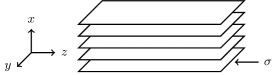
Figure 1: Geometry of the plasmonic crystal. The layered structure is periodic in the $x$-direction and consists of planar 2D metallic sheets with isotropic conductivity $\sigma$.

The material filling the space between any two consecutive sheets is described by the anisotropic relative permittivity tensor $\text{diag}\,(\varepsilon_{x},\varepsilon_{y},\varepsilon_{z})$, where $\varepsilon_{x}=\text{constant}$, and $\varepsilon_{y}(x)=\varepsilon_{z}(x)$ depends on the spatial coordinate $x$ with period $d$. Here, we set the vaccuum permittivity equal to unity, $\varepsilon_{0}=1$. We seek solutions of time-harmonic Maxwell’s equations with transverse-magnetic (TM) polarization, that is, with electric and magnetic field components ${\bm{E}}=(E_{x},0,E_{z})$ and ${\bm{H}}=(0,H_{y},0)$. The assumed TM-polarization and the symmetry of the physical system suggest that

$$E_{z}(x,z)=\mathcal{E}(x)\,e^{\mathrm{i}k_{z}z},$$

which effectively reduces the system of governing equations to a 2D problem. Substituting the above ansatz into time-harmonic Maxwell’s equations and eliminating $E_{x}$ and $H_{y}$ leads to the following ordinary differential equation for $\mathcal{E}(x)$:

$$-\partial_{x}^{2}\mathcal{E}+\kappa(k_{z})\varepsilon_{z}(x)\mathcal{E}=0,\quad\kappa(k_{z})=\frac{k_{z}^{2}-k_{0}^{2}\varepsilon_{x}}{\varepsilon_{x}},$$ (1)

where $\mu$ denotes the permeability of the ambient material and $k_{0}=\omega\sqrt{\mu}$. By the continuity of the tangential electric field and the jump discontinuity of the tangential magnetic field due to surface current, the metallic sheets give rise to the following transmission conditions at $x=nd$:

$$\begin{cases}\mathcal{E}^{+}=\mathcal{E}^{-},\\[3.00003pt] -\mathrm{i}(\omega/\sigma)\left[\big{(}\partial_{x}\mathcal{E}\big{)}^{+}-\big{(}\partial_{x}\mathcal{E}\big{)}^{-}\right]=\kappa(k_{z})\,\mathcal{E}^{+},\end{cases}$$

where $(.)^{\pm}$ indicates the limit from the right ($+$) or the left ($-$) of the metallic boundary. In order to close the system of equations, we make a Bloch-wave ansatz in the $x$-direction, with $k_{x}$ denoting the real Bloch wavenumber:

$$\mathcal{E}(x)=e^{\mathrm{i}k_{x}d}\mathcal{E}(x-d),\quad\partial_{x}\mathcal{E}(x)=e^{\mathrm{i}k_{x}d}\partial_{x}\mathcal{E}(x-d).$$

The combination of the transmission conditions and the periodicity assumption leads to a closed system consisting of Eq. (1) and the following boundary conditions:

$$\begin{bmatrix}\mathcal{E}(d^{-})\\ \mathcal{E}^{\prime}(d^{-})\end{bmatrix}=e^{\mathrm{i}k_{x}d}\begin{bmatrix}1&0\\ -\mathrm{i}(\sigma/\omega)\kappa(k_{z})&1\end{bmatrix}\begin{bmatrix}\mathcal{E}(0^{+})\\ \mathcal{E}^{\prime}(0^{+})\end{bmatrix}\;,$$

with $\mathcal{E}^{\prime}(x)=\partial_{x}\mathcal{E}(x)$.

We next describe the dispersion relation between $k_{x}$ and $k_{z}$ in general terms. In the following analysis, we work in the 2D wavenumber space with ${\bm{k}}=(k_{x},k_{z})$. To render Eqs. (1) with the above boundary conditions amenable to analytical and numerical investigation, we perform an additional algebraic manipulation: Let $\mathcal{E}_{(1)}(x)$ and $\mathcal{E}_{(2)}(x)$ be solutions of Eq. (1) with initial conditions

$$\mathcal{E}_{(1)}(0)=1,\;\mathcal{E}^{\prime}_{(1)}(0)=0,\quad\mathcal{E}_{(2)}(0)=0,\;\mathcal{E}^{\prime}_{(2)}(0)=1.$$ (2)

These solutions are linearly independent and therefore the general solution for $\mathcal{E}(x)$ is given by $\mathcal{E}(x)=c_{1}\mathcal{E}_{(1)}(x)+c_{2}\mathcal{E}_{(2)}(x)$. The existence of a non-trivial solution implies the condition

$$D[{\bm{k}}]=\det\Bigg{(}e^{\mathrm{i}k_{x}d}\begin{bmatrix}1&0\\ -\mathrm{i}(\sigma/\omega)\kappa(k_{z})&1\end{bmatrix}\\ -\begin{bmatrix}\mathcal{E}_{(1)}(d)&\mathcal{E}_{(2)}(d)\\ \mathcal{E}^{\prime}_{(1)}(d)&\mathcal{E}^{\prime}_{(2)}(d)\end{bmatrix}\Bigg{)}\;=\;0.$$ (3)

Equation (3) expresses an implicit dispersion relation, namely, the locus of points ${\bm{k}}$ such that $D[{\bm{k}}]=0$.

III An example: Parabolic dielectric profile

For certain permittivity profiles $\varepsilon_{z}(x)$ of period $d$, the system of Eqs. (1) and (2) admits exact, closed-form solutions. Thus, Eq. (3) is made explicit. Next, we present analytical and computational results for a parabolic permittivity profile $\varepsilon_{z}(x)$. Note that the case of constant permittivity, $\varepsilon_{z}(x)=\,\text{const.}$, is analyzed in Ref. Mattheakis et al., 2016.

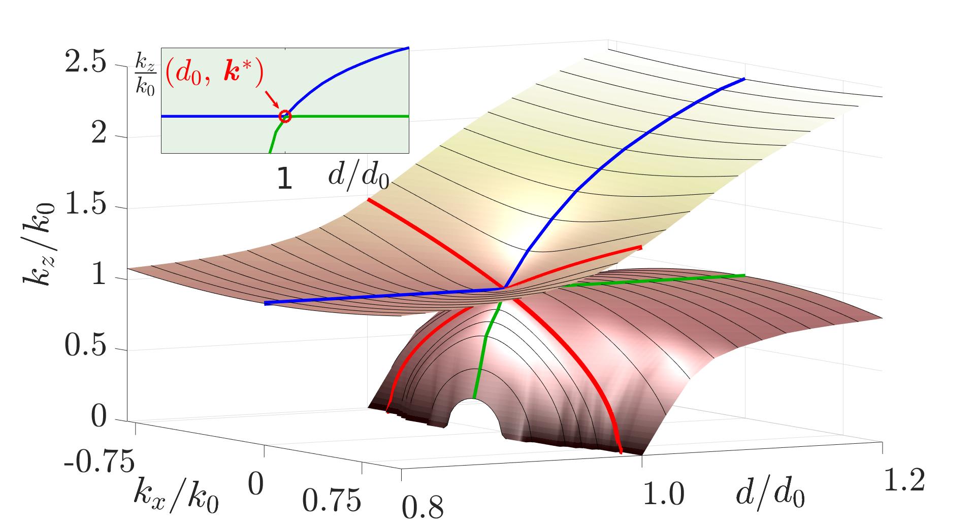
(a)

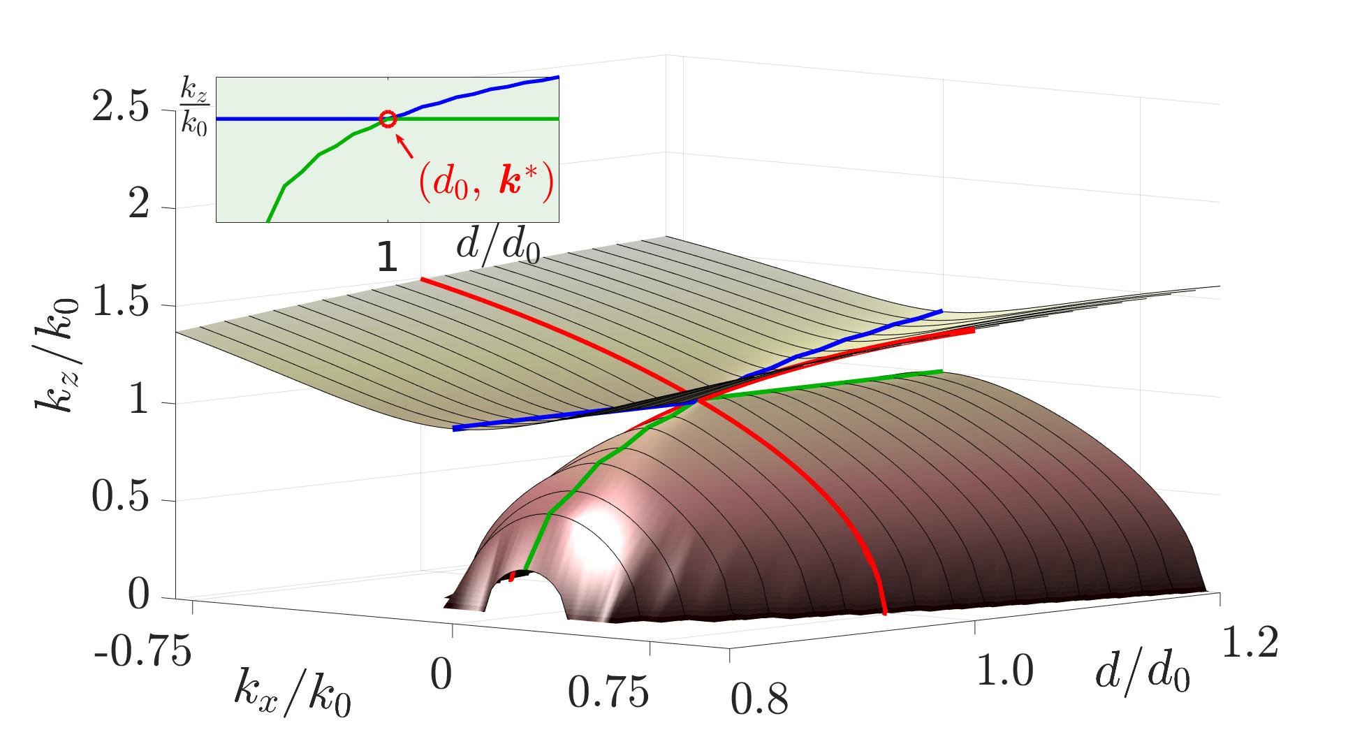
(b)

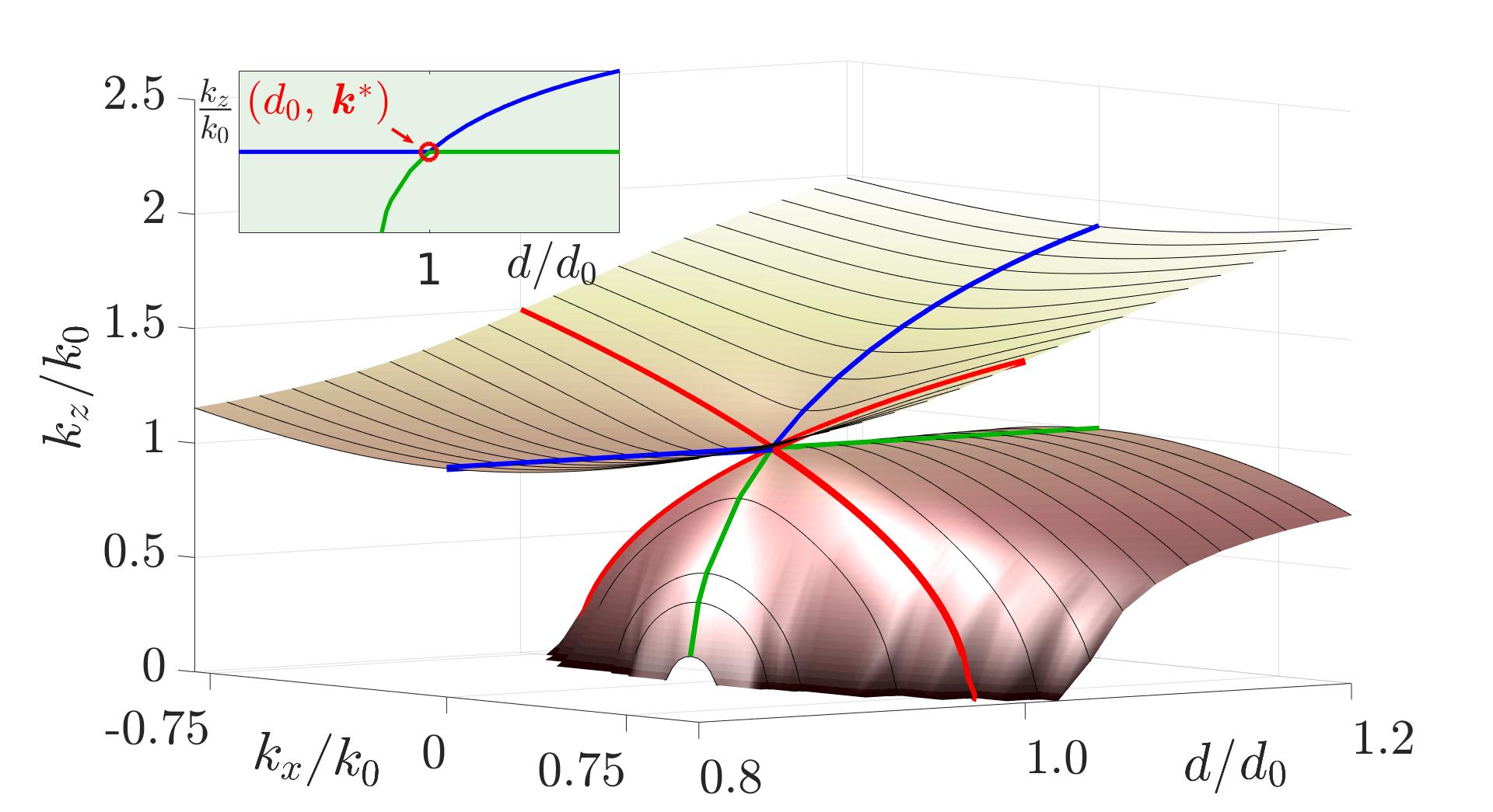
(c)

Figure 2: Parameter study of numerically computed dispersion curves for (a) the parabolic profile (4) with the scaling parameter $\alpha=20/3$, (b) double-well profile $f_{\text{dw}}$ and (c) non-symmetric profile $f_{\text{ns}}$. $d/d_{0}$ is chosen in the range from 0.8 to 1.2. The red solid lines indicate the Dirac cones dispersion at $d=d_{0}$. The inset shows the dispersion relation at the center of the Brillouin zone ${\bm{k}}^{\ast}$ as function of $d$ (blue and green cutlines in the major image).

Accordingly, consider the parabolic dielectric profile

$$\varepsilon_{z}(x)=\varepsilon_{z,0}\Big{[}1+6\,\alpha\,\frac{x}{d}\,\Big{(}1-\frac{x}{d}\Big{)}\Big{]},$$ (4)

which is well known in optics Born and Wolf (1975); Mattheakis et al. (2012). Here, $\alpha>0$ is a scaling parameter with background dielectric permittivity $\varepsilon_{z,0}>0$. In this case, $\mathcal{E}_{(1)}$ and $\mathcal{E}_{(2)}$ can be written in terms of closed-form special functions (see Appendix A). Relation (3) can be further simplified in the vicinity of the center of the Brillouin zone, where $|k_{x}d|\ll 1$, by choosing the branch of the dispersion relation containing ${\bm{k}}^{\ast}=(k_{x}^{\ast},k_{z}^{\ast})=(0,\pm k_{0}\sqrt{\varepsilon_{x}})$. As a result of this simplification, the Bloch wave sees a homogeneous medium with effective permittivity $\varepsilon=\text{diag}\,\big{(}\varepsilon_{x},\varepsilon_{z}^{\text{eff}},\varepsilon_{z}^{\text{eff}}\big{)}$. The dispersion relation is

$$\frac{k_{x}^{2}}{\varepsilon_{z}^{\text{eff}}}\;+\;\frac{k_{z}^{2}}{\varepsilon_{x}}\;=\;k_{0}^{2},\qquad\frac{\varepsilon_{z}^{\text{eff}}}{\varepsilon_{z,0}}=1+\alpha-\frac{\xi_{0}}{d}.$$ (5)

In the above, $\xi_{0}$ denotes the plasmonic thickness, $\xi_{0}=-\mathrm{i}\sigma/(\omega\varepsilon_{z,0})$ Mattheakis et al. (2016); Wang et al. (2012, 2014). Here, we assume for the sake of argument that $\sigma$ is a purely imaginary number so that $\xi_{0}$ is real valued. Below, we will provide a derivation of (5) for general profiles $\varepsilon_{z}(x)$. Dispersion relation (5) is valid in a neighborhood of ${\bm{k}}^{\ast}$. For $\varepsilon_{z}^{\text{eff}}\gtrless 0$, this relation describes an elliptic, or hyperbolic band, respectively.

The ENZ behavior is characterized by $\varepsilon_{z}^{\text{eff}}\approx 0$ in dispersion relation (5) Mattheakis et al. (2016). In the case of the parabolic profile of this section, this condition is achieved if $\xi_{0}/d=1+\alpha$. This motivates the definition of the critical ENZ structural period,

$$d_{0}=\xi_{0}/\big{(}1+\alpha\big{)}.$$ (6)

A breakdown of Eq. (5) due to $\varepsilon_{z}^{\text{eff}}=0$ is a necessary condition to observe linear dispersion and thus dispersive Dirac cones Mattheakis et al. (2016). Even though Eq. (5) is an approximate formula describing the dispersion relation in the neighborhood of ${\bm{k}}^{\ast}$, the ENZ condition $d=d_{0}$ is exact for the existence of a Dirac cone for this example of a parabolic profile.

In the case with a lossy metallic sheet, when $\sigma$ has positive real part, $d_{0}$ becomes a complex-valued number an, thus, the ENZ condition $d=d_{0}$ cannot be satisfied exactly. However, for all practical purposes, losses are typically very small such that an effective ENZ behavior can be approximately observed with the choice $d=\textrm{Re}(d_{0})$.

We now verify the effective theory given by Eqs. (5) and (6) numerically. In order to compute all real-valued dispersion bands located near ${\bm{k}}^{\ast}$, we solve the system of Eqs. (1), (2), and (3) (for details see Appendix B). We carry out a parameter study with the scaling parameter $\alpha=20/3$, background permittivity components $\varepsilon_{z,0}=2$ (in-plane) and $\varepsilon_{x}=1$ (out-of-plane), and $d/d_{0}$ in the range from 0.8 to 1.2. The numerically computed dispersion bands are shown in Fig. 2a. A band gap appears for values of $d$ different than $d_{0}$.

IV Universality of dispersion relation and ENZ condition

In this section, we address the problem of arbitrary $\varepsilon_{z}(x)$, both analytically and numerically. We claim that effective dispersion relation (5) and ENZ condition (6) are in fact universal within the model of Sec. II. This means that they are valid for any tensor permittivity $\text{diag}\,(\varepsilon_{x},\varepsilon_{z},\varepsilon_{z})$ with arbitrary, spatial-dependent $\varepsilon_{z}(x)$. To develop a general argument, we set

$$\varepsilon_{z}(x)=\varepsilon_{z,0}f(x/d),\quad f(x)>0,$$ (7)

where $f(x)$ is an arbitrarily chosen, continuous and periodic positive function. Guided by our results for the parabolic profile (Sec. III), we now make the conjecture that dispersion relation (5) still holds with the definitions

$$d_{0}=\xi_{0}\left[\int_{0}^{1}f(x)\text{d}x\right]^{-1},\quad\frac{\varepsilon_{z}^{\text{eff}}}{\varepsilon_{z,0}}=\xi_{0}\left(\frac{1}{d_{0}}-\frac{1}{d}\right).$$ (8)

In the following analysis, we give a formal bifurcation argument justifying definition (8). We start by expanding Eq. (3) in the neighborhood of ${\bm{k}}^{\ast}$ in powers of the components of $\delta{\bm{k}}=(\delta k_{x},\delta k_{z})={\bm{k}}^{\ast}-{\bm{k}}$. First, it can be readily shown that at ${\bm{k}}={\bm{k}}^{\ast}$ Eq. (1) reduces to $-\partial_{x}^{2}\mathcal{E}=0$. Thus, the system of fundamental solutions is given by $\mathcal{E}_{(1)}(x)=1$, $\mathcal{E}_{(2)}(x)=x$. This implies that $D[{\bm{k}}^{\ast}]=0$. The expansion of $D[{\bm{k}}]$ up to second order in $\delta{\bm{k}}$ leads to an expression of the form

$$D[{\bm{k}}^{\ast}+\delta{\bm{k}}]=\\ b_{x}\delta k_{x}+b_{z}\delta k_{z}+b_{xx}(\delta k_{x})^{2}+b_{zz}(\delta k_{z})^{2}+b_{xz}\delta k_{x}\delta k_{z}.$$

The occurrence of a Dirac point is identified with the appearance of a critical point for $D[{\bm{k}}]$, when $b_{x}=b_{z}=0$. In order to express $b_{x}$ and $b_{z}$ in terms of physical parameters, we notice that only the term $\big{[}\mathrm{i}e^{\mathrm{i}k_{x}d}(\sigma/\omega)\kappa(k_{z})+\mathcal{E}^{\prime}_{(1)}(d)\big{]}\,\mathcal{E}_{(2)}(d)$ of $D[(k_{x},k_{z})]$ contributes to first order in $\delta{\bm{k}}$. Accordingly, we find

$$D[{\bm{k}}^{\ast}+\delta{\bm{k}}]=\\ -d\,\Big{(}\frac{-\mathrm{i}\sigma}{\omega\varepsilon_{x}}\,2k_{z}\delta k_{z}-\delta\mathcal{E}^{\prime}_{(1)}(d)[\delta k_{z}]\Big{)}+\mathcal{O}((\delta{\bm{k}})^{2}).$$

Here, $\delta\mathcal{E}[\delta k_{z}]$ denotes the total variation of $\mathcal{E}$ with respect to $k_{z}$ in the direction $\delta k_{z}$. It can be shown (see Appendix B) that $\delta\mathcal{E}_{(1)}[\delta k_{z}]$ solves the differential equation $-\partial^{2}_{x}\delta\mathcal{E}_{(1)}=-\varepsilon_{z}(x)/\varepsilon_{x}\,2k_{z}\delta k_{z}$. The solution has the derivative

$$\delta\mathcal{E}^{\prime}_{(1)}(x)=2k_{z}\delta k_{z}\left[\varepsilon_{x}\,\int_{0}^{x}\varepsilon_{z}(\xi)\,\text{d}\xi\right]^{-1},$$

which enters $D[{\bm{k}}^{\ast}+\delta{\bm{k}}]$. Thus, we obtain $b_{x}=0$ and

$$b_{z}=\left[\xi_{0}-d\int_{0}^{1}f(x)\text{d}x\right]\frac{2dk_{z}\varepsilon_{z,0}}{\varepsilon_{x}}.$$

At the critical point, the expression in the bracket must vanish, which produces Eq. (8).

A refined computation for the critical case of $d=d_{0}$ gives $b_{xx}=-d^{2}$, $b_{xz}=0$, and $b_{zz}>0$. Thus, the effective dispersion relation at $d/d_{0}=1$ up to second-order terms is $b_{xx}\delta k_{x}^{2}+b_{zz}\delta k_{z}^{2}=0$ with $b_{xx}b_{zz}<0$, which corresponds to a Dirac cone. Moreover, for $\varepsilon_{z}^{\text{eff}}/\varepsilon_{x}\sim 1$ it can be shown that

$$D[{\bm{k}}^{\ast}+\delta{\bm{k}}]\approx-d^{2}\Big{[}\delta k_{x}^{2}+\frac{\varepsilon_{z}^{\text{eff}}}{\varepsilon_{x}}(k_{z}^{\ast}+\delta k_{z})^{2}-\frac{\varepsilon_{z}^{\text{eff}}}{\varepsilon_{x}}(k_{z}^{\ast})^{2}\Big{]}.$$

By $(k_{z}^{\ast})^{2}/\varepsilon_{x}=k_{0}^{2}$, the above relation recovers the elliptic profile of Eq. (5).

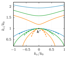
Figure 3: Numerically computed dispersion curves (solid lines) and the effective dispersion relation Eq. 5 (dashed lines) for $d/d_{0}=1.1$ computed for the parabolic (blue), double-well $f_{\text{dw}}(x)$ (orange), and nonsymmetric profile $f_{\text{ns}}(x)$ (green). The curvatures agree at the critical point ${\bm{k}}^{\ast}$.

In order to support this bifurcation argument with numerical evidence, we test Eq. (8) for two additional dielectric profiles which to our knowledge do not admit exact solutions in simple closed form. In the spirit of Ref. Roger et al., 1978, we study distinctly different profiles $\varepsilon_{z}(x)$. Specifically, we use the symmetric double-well profile $f_{\text{dw}}(x)=1-3.2x+13.2x^{2}-20x^{3}+10x^{4}$ and the non-symmetric profile $f_{\text{ns}}(x)=1+0.5\,(e^{5x}-1)(1-x)$. The computational results for the dispersion relation are given in Fig. 2b-c. Furthermore, for ${\bm{k}}$ in the neighborhood of ${\bm{k}}^{\ast}$ and $d/d_{0}=1.1$ we notice excellent agreement of effective dispersion relation (5) with the numerically computed curve $k_{z}(k_{x})$ (Fig. 3).

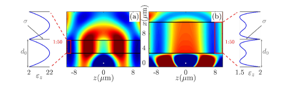
Figure 4: Spatial distribution of $H_{y}$ in an anisotropic dielectric host with 100 layers of doped graphene with structural period $d=\text{Re}(d_{0})$ (black rectangle). A magnetic dipole source is located below the multilayer structures (white dots) emitting at $f=25$ THz. The permittivity profile $\varepsilon_{z}(x)$ in (a) is a parabolic, and in (b) a double-well (insets). In the multilayer, waves propagate without dispersion and with no phase delay.

To test the results of our model against more practical configurations, we carry out direct numerical simulations for a system with a finite number of metallic sheets. We choose graphene as the material for the 2D conducting sheets, since it has been used extensively in plasmonic and optoelectronic applications Xia et al. (2014); Grigorenko et al. (2012). In the THz frequency regime, doped graphene behaves like a Drude metal because intraband transitions are dominant Grigorenko et al. (2012); Fei et al. (2012). In this frequency regime doped graphene supports plasmons Grigorenko et al. (2012). Hence, the conductivity of the metallic sheets is approximated by the Drude formula, $\sigma=\mathrm{i}e^{2}\mu_{c}/[\pi\hbar^{2}(\omega+\mathrm{i}/\tau)]$. The doping amount is $\mu_{c}=0.5$ eV and the transport scattering time of electrons is $\tau=0.5$ ps to account for optical losses Mattheakis et al. (2016); Wang et al. (2012).

In Fig. 4, we present the spatial distribution of $H_{y}(x,z)$ propagating through a structure of 100 graphene layers embedded periodically in a lossless dielectric host with anisotropic and spatial-dependent permittivity. The numerical computation is carried out for parabolic profile (4) with $\alpha=20/3$, $\varepsilon_{z,0}=2$, $\varepsilon_{x}=1$, as well as the double-well profile, with $\varepsilon_{z,0}=2$ and $\varepsilon_{x}=4$. By setting the structural period to $d=d_{0}$, we observe the expected signature of ENZ behavior, namely, wave propagation with no phase delay through the periodic structure Silveirinha and Engheta (2006); Li et al. (2015); Mattheakis et al. (2016).

V Discussion and conclusion

In this section, we conclude our analysis by discussing implications of our approach, summarizing our results and mentioning open related problems. Of particular interest is a generalization of our result for the effective dielectric permittivity of the layered plasmonic structure.

The notion of an effective permittivity $\varepsilon^{\text{eff}}_{z}$ that arises in Eqs. (5) and (8) bears a striking similarity to homogenization results for Maxwell’s equations Wellander and Kristensson (2003). In fact, it can be shown that Eq. (8) can also be derived by applying an asymptotic analysis procedure to the full system of time-harmonic Maxwell’s equations. For a general tensor-valued permittivity $\underline{\varepsilon}(x/d)$ and sheet conductivity $\underline{\sigma}(x/d)$, the effective permittivity of the metamaterial takes the form

$$\underline{\varepsilon}^{\text{eff}}=\left<\underline{\varepsilon}\,\chi\right>_{\text{host}}+\frac{\mathrm{i}}{\omega}\left<\underline{\sigma}\,\chi\right>_{\text{sheet}}.$$

Here, $\left<\,.\,\right>_{R}$ denotes the arithmetic average over region $R$ and $\chi$ is a weight function that solves a closed boundary value problem in the individual layer Maier et al. (2017). In the special case of $\underline{\varepsilon}=\text{diag}\,(\varepsilon_{x},\varepsilon_{z},\varepsilon_{z}),$ the weight function reduces to the unit tensor, $\chi=I$. Understanding the ENZ behavior on the basis of this more general effective permittivity is the subject of work in progress.

Our work points to several open questions. For example, we analyzed wave propagation through a plasmonic structure primarily in absence of a current-carrying source. A related problem is to analytically investigate how the dispersion band and ENZ condition derived here may affect the modes excited by dipole sources located in the proximity of a finite layered structure. This more demanding problem will be the subject of future work.

In conclusion, we have shown that dispersive Dirac cones are universal for a wide class of plasmonic multilayer systems consisting of 2D metals with isotropic, constant conductivity. We also derived a general, exact condition on the structural period $d$ to obtain a corresponding dispersion relation with ENZ behavior. The universality of our approach is key for the investigation of wave coupling effects in discrete periodic systems and the design of effective ENZ media. Our results pave the way to a systematic study of homogenization and effective parameters in the context of more general multilayer plasmonic systems.

Appendix A Exact solution for parabolic dielectric profile

In this appendix, we outline the derivation of the exact dispersion relation for parabolic dielectric profile (4). As a first step, we characterize the general solution of the differential equation

$$-\partial_{x}^{2}\mathcal{E}(x)+\kappa(k_{z})\varepsilon_{z}(x)\mathcal{E}(x)=0,\quad\kappa(k_{z})=\frac{k_{z}^{2}-k_{0}^{2}\varepsilon_{x}}{\varepsilon_{x}},$$

where the free space permittivity is set $\varepsilon_{0}=1$ and $k_{0}=\omega\sqrt{\mu}$. In order to derive the solution of the above differential equation, we apply a change of coordinate from $x$ to $\chi$, viz.,

$$x\to\chi=\rho\left(\frac{x}{d}-\frac{1}{2}\right),$$

using a complex-valued scaling parameter, $\rho$, to be determined below. By identifying $\tilde{}\mathcal{E}(\chi)=\mathcal{E}(x)$ the differential equation now reads

$$-\partial_{\chi}^{2}\tilde{}\mathcal{E}(\chi)+\kappa(k_{z})\varepsilon_{z,0}\frac{1}{\rho^{2}}\Big{(}1+\frac{6}{4}\alpha-6\alpha\frac{1}{\rho^{2}}\chi^{2}\Big{)}\tilde{}\mathcal{E}(\chi)=0.$$

We now fix $\rho$ by the requirement that

$$-6\alpha\frac{1}{\rho^{4}}{\kappa(k_{z})}{\varepsilon_{z,0}}=\frac{1}{4}.$$

Thus, if $\alpha\leq 0,$ we set

$$\rho(\alpha)=\Big{(}-24\,\alpha\,{\kappa(k_{z})}{\varepsilon_{z,0}}\Big{)}^{1/4}.$$ (9)

We can analytically continue the above function $\rho(\alpha)$ to values $\alpha>0$ by properly choosing one of the four branches of the (complex) multiple-valued function $w(z)=z^{1/4}$. By the definition

$$\nu=-1-\sqrt{{\kappa(k_{z})}{\varepsilon_{z,0}}}\,\frac{1+(3/2)\alpha}{(-24\alpha)^{1/2}},$$

the transformed differential equation for $\tilde{}\mathcal{E}(\chi)$ takes the canonical form

$$-\partial_{\chi}^{2}\tilde{}\mathcal{E}(\chi)+\Big{(}\frac{1}{2}\chi^{2}-\nu-\frac{1}{2}\Big{)}\tilde{}\mathcal{E}(\chi)=0.$$

This differential equation has the general solution

$$\tilde{}\mathcal{E}(\chi)=C_{1}D_{\nu}(\chi)+C_{2}D_{\nu}(-\chi),$$ (10)

where $D_{\nu}(\chi)$ is the parabolic cylinder or Weber-Hermite function, given by the formula

$$D_{\nu}(\chi)=2^{\nu/2}e^{-\chi^{2}/4}\Big{[}\frac{\Gamma(1/2)}{\Gamma(1/2-\nu/2)}\Phi\big{(}-\nu/2,1/2;\chi^{2}/2\big{)}\\ +\frac{\chi}{2^{1/2}}\frac{\Gamma(-1/2)}{\Gamma(-\nu/2)}\Phi\big{(}1/2-\nu/2,3/2;\chi^{2}/2\big{)}\Big{]},$$

and $C_{1}$ and $C_{2}$ are integration constants. In the above, $\Gamma(z)$ is the Gamma function and $\Phi(a,b;z)$ is the confluent hypergeometric function defined by the power series

$$\Phi(a,b;z)=\sum_{n=0}^{\infty}\frac{(a)_{n}}{(b)_{n}}\frac{z^{n}}{n!},$$

where $(a)_{0}=1$, $(a)_{n}=(a+n-1)(a)_{n-1}$ for $n\geq 1$.

To derive the corresponding exact dispersion relation, we need to identify the fundamental solutions $\tilde{}\mathcal{E}_{(j)}(x)$ ($j=1,2$) and then substitute general solution (10) written in terms of these $\tilde{}\mathcal{E}_{(j)}(x)$ into determinant condition (3). The resulting condition reads

$$D[{\bm{k}}] =\det\Bigg{(}e^{\mathrm{i}k_{x}d}\begin{bmatrix}1&0\\ -\mathrm{i}(\sigma/\omega)\kappa(k_{z})&1\end{bmatrix}$$

$$\quad-\begin{bmatrix}\tilde{}\mathcal{E}_{(1)}(\rho/2)&\tilde{}\mathcal{E}_{(2)}(\rho/2)\\ \tilde{}\mathcal{E}^{\prime}_{(1)}(\rho/2)&\tilde{}\mathcal{E}^{\prime}_{(2)}(\rho/2)\end{bmatrix}\Bigg{)}\;=\;0.$$

After some algebra, the exact dispersion relation reads

$$\cos(k_{x}d)+\frac{\Gamma(-\nu)}{\sqrt{2\pi}}\Big{\{}D_{\nu}(-\rho/2)D^{\prime}_{\nu}(-\rho/2)\\ +D_{\nu}(\rho/2)D^{\prime}_{\nu}(\rho/2)\\ -\frac{\kappa(k_{z})\varepsilon_{z,0}\,\xi_{0}d}{2\rho}\big{[}D_{\nu}(\rho/2)^{2}-D_{\nu}(-\rho/2)^{2}\big{]}\Big{\}}=0.$$ (11)

Here, $\xi_{0}=-\mathrm{i}\sigma/(\omega\varepsilon_{z,0})$ is the plasmonic thickness. Note that, by our construction, $\rho$ and $\nu$ are $k_{z}$ dependent, viz., $\rho=\rho(k_{z})$ and $\nu=\nu(k_{z})$. Thus, Eq. (11) still expresses an implicit relationship between $k_{x}$ and $k_{z}$. To further simplify Eq. (11), we expand $D_{\nu}(\rho/2)$ to fourth order in $z$. For sufficiently small structural period, $d$, i.e., $|\kappa(k_{z})d|\ll 1$, and after some algebraic manipulations the exact dispersion relation simplifies to

$$\cos(k_{x}d) \approx 1-\frac{\kappa(k_{z})\varepsilon_{z,0}\xi_{0}d}{2}-(2\nu+1)(-(3/2)\alpha)^{1/2}$$

$$\times\big{(}\sqrt{\kappa(k_{z})\varepsilon_{z,0}}\,d\big{)}-\frac{1}{4}\alpha\kappa(k_{z})\varepsilon_{z,0}d^{2}.$$

Furthermore, in the vicinity of Brillouin zone center, i.e., if $|k_{x}d|\ll 1$, we apply the Taylor expansion $\cos(k_{x}d)\approx 1-(1/2)\,k_{x}^{2}d^{2}$ and use the definitions of $\nu$ and $\kappa(k_{z})$ to obtain the effective dispersion relation

$$\frac{k_{x}^{2}}{\varepsilon_{z}^{\text{eff}}}\;+\;\frac{k_{z}^{2}}{\varepsilon_{x}}\;=\;k_{0}^{2},\qquad\frac{\varepsilon_{z}^{\text{eff}}}{\varepsilon_{z,0}}=1+\alpha-\frac{\xi_{0}}{d},$$

which is identical to Eq. (5).

Appendix B Numerical scheme for computation of dispersion bands

In this appendix, we present more details on the numerical procedure to compute dispersion bands for arbitrary dielectric profiles $\varepsilon_{z}(x)$. For given problem parameters $\sigma$, $\omega,$ and profile $\varepsilon_{z}(x)$, and fixed real $k_{x}$, consider the task of finding a complex-valued solution $k_{z}$ of (3).

We formulate a Newton method in order to solve the implicit dispersion relation $D[{\bm{k}}]=0$ numerically. For this purpose, we first need to characterize the variation $\delta\mathcal{E}_{(i)}$ of solutions $\mathcal{E}_{(i)}$ of Eq. (1) with respect to $k_{z}$. We make the observation that $\delta\mathcal{E}_{(i)}$ is the unique solution of the differential equation

$$-\partial_{x}^{2}\delta\mathcal{E}_{(i)}+\kappa(k_{z})\varepsilon_{z}(x)\delta\mathcal{E}_{(i)}+\kappa^{\prime}(k_{z})\varepsilon_{z}(x)\mathcal{E}_{(i)}=0,$$

where

$$\kappa^{\prime}(k_{z})=\frac{2k_{z}}{\varepsilon_{x}},$$

$$\delta\mathcal{E}_{(i)}(0)=0,\;\delta\mathcal{E}^{\prime}_{(i)}(0) =0.$$

With this prerequisite at hand, the variation of $D[{\bm{k}}]$ with respect to $k_{z}$ can be expressed as follows:

$$\delta D[{\bm{k}}]=-e^{\mathrm{i}k_{x}d}\Big{\{}\delta\mathcal{E}_{(1)}(d)\,\big{(}1-\mathcal{E}^{\prime}_{(2)}(d)\big{)}\\ +\big{(}1-\mathcal{E}_{(1)}(d)\big{)}\,\delta\mathcal{E}^{\prime}_{(2)}(d)\\ +\big{(}\mathrm{i}(\sigma/\omega)\kappa^{\prime}(k_{z})+\delta\mathcal{E}^{\prime}_{(1)}(d)\big{)}\,\mathcal{E}_{(2)}(d)\\ +\big{(}\mathrm{i}(\sigma/\omega)\kappa(k_{z})+\mathcal{E}^{\prime}_{(1)}(d)\big{)}\delta\mathcal{E}_{(2)}(d)\Big{\}}.$$ (12)

Next, we outline the steps of the Newton scheme. Let $k_{x}$ be fixed. Suppose that starting from an initial guess $k_{z}^{(0)}$ we have computed an approximate solution $k_{z}^{(n)}$ of Eq. (3). We then compute a new approximation $k_{z}^{(n+1)}$ according to the following sequence of steps:

• Solve the first order systems ($i=1,2$)

  $$\begin{cases}\begin{aligned} -\partial_{x}(\mathcal{E}^{\prime}_{(i)})+\kappa(k_{z})\varepsilon_{z}(x)\mathcal{E}_{(i)}&=0,\\ -\partial_{x}(\mathcal{E}_{(i)})&=\mathcal{E}^{\prime}_{(i)},\end{aligned}\end{cases}$$

  with initial conditions $\mathcal{E}_{(1)}(0)=1$, $\mathcal{E}^{\prime}_{(1)}(0)=0$, $\mathcal{E}_{(2)}(0)=0$, $\mathcal{E}^{\prime}_{(2)}(0)=1$.

• Solve the systems ($i=1,2$)

  $$\begin{cases}\begin{aligned} -\partial_{x}(\delta\mathcal{E}^{\prime}_{(i)})+\kappa(k_{z})\varepsilon_{z}(x)\delta\mathcal{E}_{(i)}+\kappa^{\prime}(k_{z})\varepsilon_{z}(x)\mathcal{E}_{(i)}&=0,\\ -\partial_{x}(\delta\mathcal{E}_{(i)})&=\delta\mathcal{E}^{\prime}_{(i)},\\ \partial\mathcal{E}_{(i)}(0)=0,\;\partial\mathcal{E}^{\prime}_{(i)}(0)&=0.\end{aligned}\end{cases}$$

• Compute $D[k_{x},k_{z}^{(n)}]$ and $\delta D[k_{x},k_{z}^{(n)}]$ given by Eqs. (3) and (12).

• Update:

  $$k_{z}^{(n+1)}=k_{z}^{(n)}-\frac{D[k_{x},k_{z}^{(n)}]}{\delta D[k_{x},k_{z}^{(n)}]}.$$

References

- Silveirinha and Engheta (2006) M. Silveirinha and N. Engheta, Phys. Rev. Lett. 97, 157403 (2006).
- Huang et al. (2011) X. Huang, Y. Lai, Z. H. Hang, H. Zheng, and C. T. Chan, Nat. Mater. 10, 582 (2011).
- Moitra et al. (2013) P. Moitra, Y. Yang, Z. Anderson, I. I. Kravchenko, D. P. Briggs, and J. Valentine, Nat. Photon 7, 791 (2013).
- Li et al. (2015) Y. Li, S. Kita, P. Munoz, O. Reshef, D. I. Vulis, M. Yin, M. Loncar, and E. Mazur, Nat. Photon 9, 738 (2015).
- Mattheakis et al. (2016) M. Mattheakis, C. A. Valagiannopoulos, and E. Kaxiras, Physical Review B 94, 201404(R) (2016).
- Wang et al. (2012) B. Wang, X. Zhang, F. J. García-Vidal, X. Yuan, and J. Teng, Physical Review Letters 109, 073901 (2012).
- Wintz et al. (2015) D. Wintz, P. Genevet, A. Ambrosio, A. Woolf, and F. Capasso, Nano Letters 15, 3585 (2015), pMID: 25915541.
- Dai et al. (2015) S. Dai, Q. Ma, M. K. Liu, T. Andersen, Z. Fei, M. D. Goldflam, M. Wagner, K. Watanabe, T. Taniguchi, M. Thiemens, F. Keilmann, G. C. A. M. Janssen, S.-E. Zhu, P. Jarillo-Herrero, M. M. Fogler, and D. N. Basov, Nat. Nano 10, 682 (2015).
- Nemilentsau et al. (2016) A. Nemilentsau, T. Low, and G. Hanson, Phys. Rev. Lett. 116, 066804 (2016).
- Smith (2014) D. R. Smith, Science 345, 384 (2014).
- Alù and Engheta (2005) A. Alù and N. Engheta, Phys. Rev. E 72, 016623 (2005).
- Zentgraf et al. (2011) T. Zentgraf, Y. Liu, M. H. Mikkelsen, J. Valentine, and X. Zhang, Nat. Nano 6, 151 (2011).
- Cheng et al. (2014) J. Cheng, W. L. Wang, H. Mosallaei, and E. Kaxiras, Nano Letters 14, 50 (2014).
- High et al. (2015) A. A. High, R. C. Devlin, A. Dibos, M. Polking, D. S. Wild, J. Perczel, N. P. de Leon, M. D. Lukin, and H. Park, Nature 522, 192 (2015).
- Zhukovsky et al. (2014) S. V. Zhukovsky, A. Andryieuski, J. E. Sipe, and A. V. Lavrinenko, Phys. Rev. B 90, 155429 (2014).
- Deng et al. (2015) H. Deng, F. Ye, B. A. Malomed, X. Chen, and N. C. Panoiu, Phys. Rev. B 91, 201402 (2015).
- Mirò et al. (2014) P. Mirò, M. Audiffred, and T. Heine, Chem. Soc. Rev. 43, 6537 (2014).
- Xia et al. (2014) F. Xia, H. Wang, D. Xiao, M. Dubey, and A. Ramasubramaniam, Nat. Photon 8, 899 (2014).
- Iorsh et al. (2013) I. V. Iorsh, I. S. Mukhin, I. V. Shadrivov, P. A. Belov, and Y. S. Kivshar, Phys. Rev. B 87, 075416 (2013).
- Wang et al. (2014) B. Wang, X. Zhang, K. P. Loh, and J. Teng, Journal of Applied Physics 115, 213102 (2014).
- Jablan et al. (2009) M. Jablan, H. Buljan, and M. Soljačić, Phys. Rev. B 80, 245435 (2009).
- Low et al. (2017) T. Low, A. Chaves, J. D. Caldwell, A. Kumar, N. X. Fang, P. Avouris, T. F. Heinz, F. Guinea, L. Martin-Moreno, and F. Koppens, Nat. Mater 16, 182 (2017).
- Grigorenko et al. (2012) A. N. Grigorenko, M. Polini, and K. S. Novoselov, Nat. Photon 6, 749 (2012).
- Fei et al. (2012) Z. Fei, A. S. Rodin, G. O. Andreev, W. Bao, A. S. McLeod, M. Wagner, L. M. Zhang, Z. Zhao, M. Thiemens, G. Dominguez, M. M. Fogler, A. H. C. A. H. Neto, C. N. Lau, F. Keilmann, and D. N. Basov, Nature 487, 85 (2012).
- Shirodkar et al. (2017) S. N. Shirodkar, M. Mattheakis, P. Cazeaux, P. Narang, M. Soljačić, and E. Kaxiras, Arxiv 1703.01558 (2017).
- Born and Wolf (1975) M. Born and E. Wolf, Optics and Laser Technology 7, 190 (1975).
- Mattheakis et al. (2012) M. Mattheakis, G. P. Tsironis, and V. I. Kovanis, Journal of Optics 14, 114006 (2012).
- Roger et al. (1978) A. Roger, D. Maystre, and M. Cadilhac, J. Optics (Paris) 9, 83 (1978).
- Wellander and Kristensson (2003) N. Wellander and G. Kristensson, SIAM Journal of Applied Mathematics 64, 170 (2003).
- Maier et al. (2017) M. Maier, D. Margetis, M. Luskin, M. Mattheakis, and E. Kaxiras, Paper in preparation. (2017).