Re-running the QCD shear viscosity

Abstract

The remarkably small shear viscosity to entropy density ratio $\eta/s\mathrel{\hbox to0.0pt{\lower 1.99997pt\hbox{$\sim$}\hss}\raise 1.99997pt\hbox{$<$}}0.5$ of the quark-gluon plasma (QGP) is a key insight from heavy ion experiments. Nonetheless, the basic understanding of this ‘observable’ still seems to be rudimentary, with existing perturbative QCD estimates suggesting $\eta/s\mathrel{\hbox to0.0pt{\lower 1.99997pt\hbox{$\sim$}\hss}\raise 1.99997pt\hbox{$>$}}1$ – a view that we scrutinize here.

In order to extrapolate the available perturbative approach to phenomenologically relevant temperatures, we consider carefully controllable higher-order corrections: We adapt the leading-order effective kinetic scheme (instead of the catchy next-to-leading log formula $\eta_{{}_{{\rm NLL}}}\propto[\alpha^{2}\log(c/\alpha)]^{-1}$), by using cross sections with a running coupling. This effect should be pertinent (for a QGP) and we argue for a choice of scale-dependence that makes it consistent with thermal screening.

We conclude that $\eta/s\mathrel{\hbox to0.0pt{\lower 1.99997pt\hbox{$\sim$}\hss}\raise 1.99997pt\hbox{$<$}}0.5$ does not indicate genuine non-perturbative effects, it may rather be understood within resummation-improved perturbative QCD, with some uncertainties from deploying kinetic theory near to its limit.

1 Introduction

Quantifying the shear viscosity $\eta$ of the quark-gluon plasma is a key issue in heavy-ion physics, and has been ever since RHIC and LHC experiments revealed it to be an (almost) perfect fluid Teaney2003a . Successful descriptions of the data favour a small viscosity to entropy ratio, $\eta/s\mathrel{\hbox to0.0pt{\lower 1.99997pt\hbox{$\sim$}\hss}\raise 1.99997pt\hbox{$<$}}0.5$: the hallmark for a ‘strongly coupled’ system. This feature of many-body QCD, along with the associated puzzle of rapid thermalisation, is not yet properly understood and remains a challenge to explain theoretically Danielewicz1985 .

A strong-coupling calculation for certain supersymmetric Yang-Mills theories gives $\eta/s=1/(4\pi)\approx 0.1$ Kovtun2005 , which appears to be in the right ballpark. This value was conjectured as a universal lower bound for conformal gauge theories, but digresses from real-world QCD Huot2007 . Moreover, it does not reveal anything about the temperature dependence of $\eta$ in a QGP. Certain models for $\eta(T)$ can be eliminated by comparing hydrodynamic output to transverse particle spectra and elliptic flow Niemi2015qia ; Denicol2016 . Ongoing lattice computations have helped extract $\eta(T)$ for a gluonic system near $T_{c}$, by reverse-engineering the Green-Kubo formulae. However, the assumed form of the spectral function does not respect asymptotic freedom Meyer2007f ; Meyer2009e ; Mages2015 ; Astrakhantsev2017 .

First principle perturbation theory is apparently at odds with the small viscosity, commonly reckoned to imply that all ‘weak-coupling’ approaches are inadequate. Actually, this point of view is misleading as it follows from an incomplete approximation. We show how an asymptotic weakening of the strong interaction, when treated consistently at the 1-loop level, leads to a natural explanation for the low values of $\eta/s$.

Kinetic theory ought to give quantitative estimates for transport properties provided the mean free path length $\lambda$ (specified by the associated cross section) exceeds the inter-particle distance Reif1964 . The viscosity is given by ($\iota\approx 1/3$ is a numerical factor)

$$\eta\simeq\iota\cdot n\bar{p}\lambda$$ (1)

from the density of particles $n$ which can transfer a typical momentum $\bar{p}$ over a distance $\lambda\mathrel{\hbox to0.0pt{\lower 1.99997pt\hbox{$\sim$}\hss}\raise 1.99997pt\hbox{$>$}}n^{-1/3}$. For gauge theories it is important to distinguish between the total cross section and $\sigma_{\rm tr}=\int d\Omega\,(1-\cos\theta)\,d\sigma/d\Omega$. Relevant for the viscosity is the latter, the so-called transport cross section, which takes into account that a single one of the prevailing small-angle scatterings is not sufficient to transfer the typical momentum $\bar{p}\sim T$ (for relativistic plasmas). Although the ‘transport weight’ $(1-\cos\theta)$, which is proportional to the invariant momentum exchange $t$, does reduce the sensitivity of the viscosity to the infrared sector, it is still mandatory to also take into account quantum corrections in order to obtain non-trivial results. E. g., for $t$-channel boson exchange (see Fig. 1) with $d\sigma/dt\sim\alpha^{2}/t^{2}$ at tree-level, the transport cross section is logarithmically divergent, arising from the integral $\int_{-s}^{t_{\rm max}}dt/(-t)$. Due to the kinematic boundary $t_{\rm max}=0$, the viscosity would be zero (in fact for any value of the bare coupling). However, the exchanged boson acquires a self-energy of the order $\mu^{2}\sim\alpha T^{2}$ due to thermal fluctuations which cannot be omitted in particular for $t\to 0\,$. For small coupling $\alpha$, $\mu^{2}$ is well separated from the typical invariant collision energy $s\sim T^{2}$. Thus $\sigma_{\rm tr}$ can be ‘mimicked’ by an unscreened differential cross section, integrated over a restricted $t$-range,

$$\sigma_{\rm tr}\sim\frac{1}{s}\int_{-s}^{-\mu^{2}}dt\,|t|\,\frac{\alpha^{2}}{t^{2}}\sim\frac{\alpha^{2}}{T^{2}}\log\left(\alpha^{-1}\right)\,.$$ (2)

The emerging leading logarithm (LL) indicates the screening of soft scatterings due to loop corrections. While details of the regulator $\mu^{2}$ do not affect the LL prefactor, they determine the argument of the logarithm, giving subleading terms ${\cal O}(\alpha^{2})$ in Eq. (2). We emphasize that the argument $\alpha^{-1}$ of the characteristic Coulomb logarithm is a ratio of ‘hard’ and ‘soft’ scales.

Figure 1: Gluon-gluon scattering in the $t$-channel at LO produces a large forward peak in $d\sigma/dt$ due to the long range of ‘glancing’ interactions (a $u$-channel process contributes similarly by crossing). With $P=(E,\mbox{\boldmath$p$})$ denoting the four-momenta, we label the colliding partners as $\{P_{1},P_{2}\}\rightarrow\{P_{3},P_{4}\}$. The exchanged gluon (carrying 4-momentum $Q=P_{1}-P_{3}$ and thus $t=Q^{2}$) is dressed by interactions with the medium, as a minimal requirement for the LL result.

The corresponding path length is $\lambda\sim(n\sigma_{\rm tr})^{-1}\sim 1/(T\alpha^{2}\log(\alpha^{-1}))$, where we used $n\sim T^{3}$ for the particle density. Since $n$ is also proportional to the entropy density, (1) gives the parametric $\alpha$-dependence

$$\eta/s\sim\bar{p}\lambda\sim 1/\left(\alpha^{2}\log(\alpha^{-1})\right)$$ (3)

for hot gauge theories.

We briefly summarise the history of $\eta$ calculations: first attempts were based on the relaxation time approximation of the Boltzmann equation Hosoya1985a . Those estimates were improved by Baym and collaborators who linearised the QCD Boltzmann equation with the collision term screened with hard thermal loop (HTL) insertions Baym1990 ; Heiselberg1994b . This fixed the overall prefactor in (3), to give the LL result. As it turned out, inelastic processes (naïvely of higher order in $\alpha$) need be included to go beyond the LL approximation. This was recognized by Arnold, Moore and Yaffe Arnold2000d , who subsequently calculated the coefficient $c$ in the next-to leading log (NLL) and state-of-the-art result Arnold2003f

$$\eta_{{}_{\mathrm{NLL}}}=\frac{bT^{3}}{\alpha^{2}\log(c/\alpha)}\,.$$ (4)

The constants $b$ and $c$ were computed numerically, for various number of flavors $n_{\!f}\,$, from the leading order (LO) fixed-coupling result, $\eta_{{}_{\mathrm{LO}}}^{\rm fix}$, obtained in the effective kinetic framework Arnold2003a ; in the quenched limit $b\simeq 0.34$ and $c\simeq 0.61$.

In general, $\eta(\alpha)$ is a decreasing function as expected on physics grounds: velocity gradients should equilibrate more efficiently by stronger interactions (unless the quasiparticle structure of the system changes, like in phase transitions). This expectation is indeed met by the NLL result (4) for small $\alpha$, where it is strictly justified. However, $\eta_{{}_{\mathrm{NLL}}}(\alpha)$ has a minimum at $\alpha^{\star}=c/\sqrt{e}$ ($e$ is Euler’s number). Numerically, $\min\left[\eta_{{}_{\mathrm{NLL}}}\right]=2beT^{3}/c^{2}$ turns out to be close to the free entropy $s_{0}=(16+\frac{21}{2}n_{\!f})\frac{4\pi^{2}}{90}T^{3}$, which overestimates the entropy of the interacting QGP (in particular near the confinement transition). Thus it is plain that the NLL result (4) is incompatible with $\eta/s\mathrel{\hbox to0.0pt{\lower 1.99997pt\hbox{$\sim$}\hss}\raise 1.99997pt\hbox{$<$}}0.5$ – which may have led to the common view that perturbative QCD cannot explain the experimental findings. In order to scrutinize this position, we may see the minimum at $\alpha^{\star}$ as a precursor to the singularity of $\eta_{{}_{\mathrm{NLL}}}(\alpha)$ at $\alpha=c$, which marks the ultimate break-down of the NLL approximation. However, as is obvious from the derivation of the parametric formula (3), this singularity is unphysical because it stems from a swapping of integration bounds in (2), where screening was taken into account by modifying $t_{\rm max}=0\to-\mu^{2}$. This suggests that also the minimum of $\eta_{{}_{\rm{NLL}}}$ is an artefact, which will motivate us to withhold the expansion in powers of $\log(1/\alpha)$, focusing instead on the full (unexpanded) LO result.

As a monotonously decreasing function, we shall find that $\eta_{{}_{\rm{LO}}}(\alpha)$ could potentially explain $\eta/s\mathrel{\hbox to0.0pt{\lower 1.99997pt\hbox{$\sim$}\hss}\raise 1.99997pt\hbox{$<$}}0.5$ – depending on the value chosen for $\alpha$. But specifying $\alpha$ should not be guesswork. The running of the coupling is determined by the vacuum parts of the very same quantum corrections whose thermal counterpart we have emphasized to be mandatory for screening, and thus for any reasonable approximation of transport observables like $\eta$. Of course, for renormalisation-group invariant approximations, the choice of ‘the’ scale of the running coupling $\alpha(Q)$ is arbitrary: rescaling $Q\to\widetilde{Q}$ is compensated by emerging $\alpha(\widetilde{Q})\log(\widetilde{Q}/Q)$ correction terms. These terms should either be included explicitly, or be minimized by a ‘natural’ choice of scale for the relevant processes. For the important $t$-channel process in Fig. 1, which leads to (2), this natural scale will be $Q^{2}\sim t$. Otherwise, ad hoc choices like $Q=2\pi T$ may result in considerable inaccuracies, in particular for a quantity like $\eta$, which depends on the square of the coupling.

Our paper is organised as follows. To begin with, in Sec. 2, we elaborate on the existing approximations and their range of validity. From a simple model (based on the NLL result) we can make a judgement on the extrapolation of $\eta_{{}_{\mathrm{LO}}}$ to larger values of the fixed coupling. Section 3 is where we turn QCD particularities and address the question of scale setting for the running coupling. Our results for $\eta(T)$ are given in Sec. 4, where we also combine it with the lattice entropy to estimate $\eta/s$ for $T\sim T_{c}$ and then comment on kinetic theory in Sec. 4.2.

2 Remarks on the existing calculation

Screening is the basic mechanism necessary to calculate typical transport properties, which amounts to resuming at least the 1-loop selfenergy in the propagators. Whether higher loop corrections will give more reliable approximations, or not, is a relevant question, given that perturbative series do not converge. In quantum field theories we may at best expect asymptotic expansions. While not being convergent, they can still constitute useful approximations if truncated at an appropriate ‘optimal’ order, which usually becomes smaller with increasing coupling strength ItzyksonZuber . Thus, striving for more than the 1-loop insertions absolutely necessary for screening may not result in more reliable approximations for transport phenomena in heavy-ion physics, which are characterized by a ‘fairly large’ coupling. Complementing the ‘1-loop screening’ by collinear $1\to 2$ splitting processes defines the framework of the LO effective kinetic theory developed in Arnold2003f that allowed the values $b$ and $c$ in (4) to be computed. In order to extract the LO transport properties in this effective kinetic theory it is sufficient to dress only the infrared sensitive scattering amplitudes for soft momenta. One may then calculate transport properties for arbitrarily small $\alpha(T)$, which (with the above motivation) make for a prudent compromise on which to base estimates at larger coupling. Regardless, it is the only feasible calculation scheme available at present.

Using HTL perturbation theory has the virtue of gauge invariance but presumes that soft and hard scales are well separated, $\mu^{2}\ll T^{2}$. This aspect will dominate the uncertainties when extrapolating the approach to larger coupling: Our estimates in Sec. 2.1 indicate that the HTL approximation gives a factor of two uncertainty for the viscosity at larger coupling. We may therefore simplify the approach in other aspects. First, we may omit the inelastic processes [which lead to ${\cal O}(5\%)$ higher scattering rates, thus mildly lowering $\eta$]. We may also solve in Sec. 2.2 the linearized Boltzmann equation by a suitable single-function Ansatz (which already gives an accuracy of $\mathrel{\hbox to0.0pt{\lower 1.99997pt\hbox{$\sim$}\hss}\raise 1.99997pt\hbox{$<$}}1\%$ Heiselberg1994b ), instead of a full variational treatment. The validity of a kinetic approach per se at larger coupling will be discussed in Sec. 4.2.

2.1 An effective model

Given that the non-monotonous behavior of $\eta_{{}_{\mathrm{NLL}}}(\alpha)$ is related to a sharp cut-off in the $t$-integral (2) for the derivation of the parametric form (3) of the viscosity, we are inspired to study

$$\sigma^{\rm toy}_{\rm tr}(s,\mu^{2})\ = \int_{-s}^{0}dt\,\frac{|t|}{2s}\,\frac{\alpha^{2}}{(t-\mu^{2})^{2}}\ =\ \frac{\alpha^{2}}{2s}\Big{[}\,\log\left(\frac{s}{\mu^{2}}+1\right)-\frac{s}{s+\mu^{2}}\,\Big{]},$$ (5)

using a ‘self-energy’ $\mu^{2}\sim\alpha T^{2}$ instead of a sharp cut-off. Earlier we tentatively assumed that the typical invariant energy for the transport cross section in a thermal medium is hard, $s\sim T^{2}$ (which seems to be a reasonable view in the given context).

However, the gist of the somewhat technical framework outlined in Section 2.2 is that the viscosity is approximately a convolution of the screened transport cross section with a positive function which, with appropriate normalization, can be interpreted as a probability for momentum exchange between laminar layers,

$$\frac{\eta}{T^{3}}\simeq 1\Big{/}\int ds\,sP(s)\cdot\sigma_{\rm tr}(s)\,.$$ (6)

The simple scheme (5), (6) will allow us to discuss several aspects of extrapolations to larger coupling strength. By matching it for weak coupling to the perturbative QCD result (4), we can readily infer the normalisation $2\int dsP(s)=b^{-1}$. In order to match also the constant $c$ in (4) we adjust the regulator $\mu^{2}=\kappa\cdot 4\pi\alpha T^{2}$: From (39) we find $\kappa\simeq 0.38/c\simeq 0.62$, i. e. $\mu^{2}$ is somewhat smaller than the Debye mass-squared, $m_{D}^{2}=4\pi\alpha T$. This procedure not only takes into account the remaining elastic contributions in the binary QCD cross section ($t$ and $u$ channels contribute equally by crossing symmetry), but also inelastic processes (which give only a small correction, as noted before). Figure 2 shows that our effective model agrees well the LO QCD result Arnold2003f (reviewed in the next section) even for large coupling well beyond the breakdown of the NLL result (4).

Figure 2: The QCD shear viscosity in the quenched limit as a function of fixed coupling strength, in NLL approximation (4) and to LO Arnold2003f . The latter is well reproduced by the model (5), (6), which allows to estimate the sensitivity on the screening of hard interactions, see text. For comparison, the hatched region demarcates the entropy between the LO result $s_{{}_{\rm LO}}=s_{0}(1-\frac{15}{4\pi}\alpha)$ and the free limit.

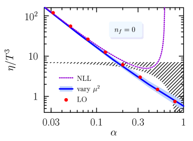
Having specified the model, we can now estimate the uncertainties that must be faced in QCD when using HTL-dressed propagators, by studying the sensitivity of the viscosity (6) on the ‘self-energy’ at harder momentum transfers. Varying $\mu^{2}$ by factors $\nu=2^{\pm 1/2}$ for $|t|>T^{2}$ has only a mild effect: Even for $\alpha\sim 1$ the viscosity changes by less than a factor of $\nu^{-1}$, cf. Fig. 2.

Alternatively, we could also segregate momentum transfers at $t^{\star}\in[-s,0]$, and set $\mu^{2}\to 0$ for $|t|>|t^{\star}|$, i. e. use the Born cross section for harder interactions, which is basically the Braaten-Yuan method Braaten1991d ,

$$\int_{-s}^{t^{\star}}dt\frac{|t|}{2s}\frac{\alpha^{2}}{t^{2}}\ +\ \sigma_{\rm tr}^{\rm toy}\big{(}-t^{\star},\mu^{2}\big{)}=\frac{\alpha^{2}}{2s}\Big{[}\,\log\Big{(}\,\frac{s}{\mu^{2}}-\frac{s}{t^{\star}}\,\Big{)}-\frac{t^{\star}}{t^{\star}-\mu^{2}}\,\Big{]}\,.$$ (7)

The resulting viscosity is $t^{\star}$-independent only at NLL order. The sub-leading terms lead to a $t^{\star}$-dependence which becomes more pronounced for increasing $\alpha$. Varying $|t^{\star}|$ in the range $[\frac{1}{2},2]T^{2}$, we observe a similar sensitivity as above on $\nu$, leading us to estimate that the HTL approximation does not bring more than a factor of two uncertainty for the viscosity calculation.

While the full (unexpanded) RHS of (5) is obviously a manifestly positive, monotonously decreasing function of $\mu^{2}/s\sim\alpha$, its NLL approximation, $\sigma_{\rm tr}^{{}_{\mathrm{NLL}}}/\alpha^{2}=s^{-1}[\log(s/\mu^{2})-1]$, becomes negative for $s/\mu^{2}<e$, leading to the same unphysical behavior as seen in (2) and (4). This problem is not cured by higher order terms since the expansion has a radius of convergence $\mu^{2}/s=1$, stemming from the pole of ${\cal M}\sim\alpha/(t-\mu^{2})$ at $t=\mu^{2}$ (off the physical sheet) in the integrand of (5). The factor of $|t|$ cedes a branch cut on the negative real axis $s<-\mu^{2}$, rather than a pole at $s=-\mu^{2}$ in $\sigma=\int dt\,d\sigma/dt$, and expansions only converge in the disk of radius $\mu^{2}$, illustrated in Fig. 3. Therefore the powers of $\mu^{2}/s$, formally beyond LO, should be considered carefully when extrapolating to larger coupling.

Figure 3: Panel (a) shows how the transport cross section in (5) depends on $s/\mu^{2}$. The NLL approximation, $\sigma_{\rm tr}^{\rm NLL}\sim\log(s/\mu^{2})$ is accurate for $s\gg\mu^{2}$, guaranteed for weak coupling $\alpha\to 0$. However an expansion in $\mu^{2}/s\sim\alpha$ extrapolates poorly (family of gray curves) for ‘soft’ $s$, where $\sigma_{\rm tr}\approx\alpha^{2}s/(2\mu^{4})$. In the complex $s$-plane, $\sigma_{\rm tr}$ has a branch cut on the negative real axis for $s<-\mu^{2}$. Thus, shown in (b), the radius of convergence is $\mu^{2}$.

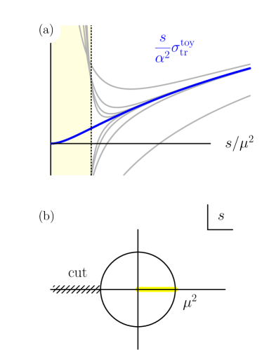
To substantiate this statement, and deferring proof to Appendix A, we point out that $P(s)$ is non-zero for $s\to 0$. Thus, expanding $\sigma_{\rm tr}$ in $\mu^{2}/s\sim\alpha T^{2}/s$ before convoluting it with $P(s)$ in Eq. (6) yields an ill-defined series in powers of $\alpha$: its coefficients [the negative moments of $P(s)$] are IR-divergent, with increasing severity. Interchanging expansion and integration is formally not permissible given the properties of the particle’s local equilibrium distribution encoded in $P(s)$. This issue is generic; the non-monotonous behavior of $\eta_{{}_{\mathrm{NLL}}}(\alpha)$ is a mathematical artifact rather than a breakdown of perturbative QCD per se. It also means that these higher order by-products must be kept.

2.2 Linearised Boltzmann equation

Having elaborated on the quality of various approximations and their respective drawbacks, we turn to the rigorous kinetic theory for QCD. What was established in Refs. Baym1990 ; Heiselberg1994b ; Arnold2000d ; Arnold2003f can guide us to (6), which we explain here for the quenched limit ($n_{\!f}=0$).

We characterise the system by $f(\mbox{\boldmath$p$},\mbox{\boldmath$x$},t)$, the number of partons in the phase-space element $d^{3}\mbox{\boldmath$p$}d^{3}\mbox{\boldmath$x$}/(2\pi)^{3}$. The evolution of $f$ can be described by the Boltzmann equation,

$${\cal D}f={\cal C}\left[f\right]\,,$$ (8)

where the streamline derivative ${\cal D}=\partial_{t}+\mbox{\boldmath$v$}\mbox{\boldmath$\nabla$}$ for relativistic particles. For binary scatterings (see Fig. 1) the collisional operator reads

$${\cal C}\left[f_{1}\right](p_{1}) = \frac{1}{2E_{1}}\int d\Gamma\left|{\cal M}\right|^{2}\big{\{}\ \bar{f}_{1}\bar{f_{2}}f_{3}f_{4}-f_{1}f_{2}\bar{f_{3}}\bar{f_{4}}\ \big{\}}\,,$$

using the subscript on the distribution function to refer to its momentum argument, $f_{i}=f(\mbox{\boldmath$p$}_{i})$. Quantum effects are included by the bracketed term (2.2); we use the notation $\bar{f}=1\pm f$, with the upper sign for bosons and the lower for fermions. Two-body phase space is abbreviated

$$\int d\Gamma\ \equiv \ d_{2}\int_{234}\frac{(2\pi)^{4}}{8E_{2}E_{3}E_{4}}\delta^{(4)}\left(P_{1}+P_{2}-P_{3}-P_{4}\right)\,,$$

using the shorthand $\int_{i}=\int d^{3}p_{i}/(2\pi)^{3}$; with $d_{g}=16$ and $d_{q}=12n_{\!f}$ being the gluon and quark degeneracies for $n_{\!f}$ light flavours respectively. Note that $\int d\Gamma$ is a Lorentz invariant measure with $P=(E,\mbox{\boldmath$p$})$ being the usual 4-momentum. In (2.2), the matrix element $|{\cal M}|^{2}$ is averaged over spin and colour of incoming particles $\{1,2\}$, but summed over final states $\{3,4\}$ (taking into account double counting). In vacuum at Born level, ${\cal M}$ is dependent only on the Mandelstam invariants [we use the ${\rm Diag}(1,-\mbox{\boldmath$1$})$ convention for the metric]

$$s=(P_{1}+P_{2})^{2}\,,\quad t=(P_{1}-P_{3})^{2}\,,\quad u=(P_{1}-P_{4})^{2}\,.$$

A heat bath in equilibrium (which is static and uniform in $x$) has a collective flow and is characterised by a temperature $T$ and velocity $u$. The Jüttner distribution function

$$f_{\rm eq}\left(\mbox{\boldmath$p$}\,;T,\mbox{\boldmath$u$}\right) = \left(e^{\displaystyle\gamma(p-\mbox{\boldmath$p$}\mbox{\boldmath$u$})/T}\mp 1\right)^{-1}\,,$$ (9)

where $\gamma=\left(1-u^{2}\right)^{-1/2}$, solves (8) trivially since ${\cal C}\left[f_{\rm eq}\right]=0$ . Consider now small deviations from the global equilibrium in (9), by allowing for $u$ to weakly depend on $x$ and consider as an Ansatz to solving (8) the function $f(\mbox{\boldmath$x$},\mbox{\boldmath$p$})=f_{\rm eq}\mbox{\boldmath$($}\mbox{\boldmath$p$}\,;\mbox{\boldmath$u$}(\mbox{\boldmath$x$})\mbox{\boldmath$)$}$, the so called ‘local’ equilibrium [to be distinguished from the general off-equilibrium solution, $f_{\star}$]. Small gradients in the collective flow $u$ allow us to assume also that $|\mbox{\boldmath$u$}|\ll 1$, by boosting into the local rest frame. This implicit dependence of $u$ on $x$ means that $f$ no longer satisfies the Boltzmann equation (8), since

$${\cal D}f_{\rm eq}\mbox{\boldmath$\big{(}$}\mbox{\boldmath$p$}\,;\mbox{\boldmath$u$}(\mbox{\boldmath$x$})\mbox{\boldmath$\big{)}$} = S\,\Big{(}\hat{p}_{i}\hat{p}_{j}-\frac{1}{3}\delta_{ij}\Big{)}\cdot\nabla_{i}u_{j}\,,\quad{\rm with}\quad S(p)\ \equiv\ f\bar{f}\frac{p}{T}\,,$$ (10)

while the collision operator in the Boltzmann equation (8), still vanishes. Thus, the actual solution to (8) should somewhat depart from local equilibrium,

$$f_{\star}(\mbox{\boldmath$x$},\mbox{\boldmath$p$}) = f\big{(}\mbox{\boldmath$x$},\mbox{\boldmath$p$}\big{)}+\delta f(\mbox{\boldmath$p$})\,,$$

with $\delta f$ being proportional to the generic velocity gradient $\nabla_{i}u_{j}$, in order for the collision operator ${\cal C}[f_{\star}]$ to compensate (10). Let us parametrise $\delta f$ in the form, similar to Baym1990 ,

$$\delta f = f\bar{f}\ \frac{\chi^{ij}(\mbox{\boldmath$p$})}{T}\cdot\nabla_{i}u_{j}\,,$$

where the rank-2 traceless tensor $\chi^{ij}$ is

$$\chi^{ij} = \chi(p)\Big{(}\hat{p}^{i}\hat{p}^{j}-\frac{1}{3}\delta^{ij}\Big{)}\,,$$ (11)

in terms of a scalar function $\chi(p)$. The tracelessness of $\chi^{ij}$ will imply zero bulk viscosity, isolating only the shear modes.

The deviation $\delta f$ from local equilibrium (alternatively $\chi$), leads to a modification of the stress tensor from the non-interacting limit,

$${\cal T}_{ij}^{\star} = d_{g}\frac{\pi^{4}}{90}T^{4}\delta_{ij}+{\cal T}_{ij}[\delta f]$$

From (11), the first order correction (in laminar gradients) takes the conventional form

$$d_{g}\int_{p}\frac{p_{i}p_{j}}{p}\delta f(\mbox{\boldmath$p$}) = -\eta\cdot\Big{(}\,\nabla_{i}u_{j}+\nabla_{j}u_{i}-\frac{2}{3}\delta_{ij}\mbox{\boldmath$\nabla$}\mbox{\boldmath$u$}\,\Big{)}\,,$$ (12)

where the shear viscosity is now derivable from $\chi$ :

$$\eta = \frac{1}{15}d_{g}\int_{p}\chi S\,.$$ (13)

But before formula (13) may be of any use, the unknown function $\chi$ needs to be determined – under the simplifying assumption of small gradients in velocity. The left hand side of the Boltzmann equation (8), which controls the effective particle rate, is (to first order in the gradients) ${\cal D}(f+\delta f)\simeq{\cal D}f$, i. e. the convective derivative is approximated by (10). On the other hand, Ansatz (11) gives

$${\cal C}\left[f_{1}\right] \simeq \frac{\nabla_{i}u_{j}}{2TE_{1}}\int\!d\Gamma|{\cal M}|^{2}f_{1}f_{2}\bar{f_{3}}\bar{f_{4}}\cdot\Delta^{ij}\left[\chi_{1}\right]\,,$$ (14)

where (having kept terms proportional to the gradient)

$$\Delta^{ij}\left[\chi_{1}\right]\ \equiv \ \big{\{}\ \chi_{1}^{ij}+\chi_{2}^{ij}-\chi_{3}^{ij}-\chi_{4}^{ij}\ \big{\}}\,.$$

Since $\nabla_{i}u_{j}$ was arbitrary, we may use the Boltzmann equation to match (10) with (14) and hence replace $\nabla_{i}u_{j}$ by $\hat{p}_{i}\hat{p}_{j}$ to find

$$S(p) = {\cal C}_{L}\left[\chi\right](p)\,.$$ (15)

In this relation, the linearised collisional operator is defined by

$${\cal C}_{L}\left[\chi_{1}\right] \equiv \frac{3\hat{p}_{1}^{i}\hat{p}_{1}^{j}}{4E_{1}}\int\!d\Gamma|{\cal M}|^{2}f_{1}f_{2}\bar{f_{3}}\bar{f_{4}}\cdot\Delta^{ij}\left[\chi_{1}\right]\,,$$

where $\chi_{i}=\chi(p_{i})$ is an arbitrary scalar function [we reserve $\chi^{\star}$ for the actual solution of (15)]. Note that $\Delta^{ij}[\chi]$ is traceless, a property inherited directly from (11), and therefore

$$\int_{p}\chi{\cal C}_{L}\left[\chi\right] = \frac{3}{8}\int_{1}\frac{f_{1}}{2E_{1}}\int\!d\Gamma|{\cal M}|^{2}f_{2}\bar{f_{3}}\bar{f_{4}}\cdot\Big{(}\Delta^{ij}\left[\chi_{1}\right]\Big{)}^{2}\,,$$ (16)

where symmetry of the integrand was used to complete the square for $\Delta^{ij}$. Therefore ${\cal C}_{L}$ is a positive semidefinite operator, over the Hilbert space of $\chi$-functions, which vanishes only for collisionally conserved quantities.

Eq. (15) then determines $\delta f$ [via $\chi(k)$], enabling (13) to be used formally with the exact solution: $\chi^{\star}={\cal C}_{L}^{-1}\left[S\right]$. One approach to solving this symbolic equation is to represent $\chi$ by a linear combination over some complete set of functions. Since ${\cal C}_{L}$ is linear, this would produce an (algebraic) matrix equation which may be solved for the coefficients. Such a strategy, using a truncated basis, gives a lower estimate for $\eta$ as we now explain.

Consider the quadratic functional, following Arnold2000d ,

$${\cal Q}\left[\chi\right] = d_{g}\int_{p}\Big{(}S\chi-\frac{1}{2}\chi{\cal C}_{L}\left[\chi\right]\Big{)}\,.$$ (17)

At $\chi^{\star}$, the solution to (15) , ${\cal Q}$ takes the value $\eta$ (up to a prefactor). The linearised Boltzmann equation is tantamount to

$$\frac{\delta{\cal Q}}{\delta\chi} = 0\,,$$

and is solved by $\chi^{\star}$, where ${\cal Q}$ is stationary. Because ${\cal C}_{L}$ is positive definite, see (16), the extremum of (17) at $\chi=\chi^{\star}$ is in fact a maximum. Its value here, on account of Eq. (13), gives the viscosity:

$$\eta = \frac{2}{15}{\rm Max}\big{(}{\cal Q}\big{)}\,,$$ (18)

which sidesteps the task of actually inverting ${\cal C}_{L}$. For example, the optimal norm of any test function may be derived from $\partial_{A}{\cal Q}\left[A\chi\right]=0$, which in a sense ‘homogenises’ (17). We may then substitute ${\cal Q}$ with the following (improved) estimate,

$${\cal Q}[\chi] = \frac{\displaystyle\Big{(}d_{g}\int_{p}S\chi\Big{)}^{2}}{\displaystyle 2d_{g}\int_{p}\chi{\cal C}_{L}\left[\chi\right]}\,.$$ (19)

If (19) is used for ${\cal Q}$ instead of Eq. (17), the absolute scale of $\chi$ is arbitrary (evidently it cancels out in the fraction). This functional, along with the known QCD matrix element for gluon-gluon scattering (with IR terms aptly screened), enables $\eta$ to be calculated accurately from a suitably adjusted test function $\chi$. Appending the quark sector is a technicality which allows for ‘mixing’ between boson and fermion distributions (E.g. due to fusion reactions like $gg\leftrightarrow q\bar{q}$). To evaluate $\eta$ for a general $n_{\!f}>0$, we refer the reader to the cross section listing in Table III of Ref. Arnold2003f . Numerical determination of $\int_{p}\chi{\cal C}_{L}[\chi]$ involves the phase space integration over all collisional momenta subject to energy and momentum conservation. See Appendix C for our covariant manipulation of the resulting 5-fold integral (which in general cannot be reduced further).

Connecting to Eq. (6)

In order to validate our effective $t$-channel model in Sec. 2.1, we show how Eq. (19) leads naturally to (6). The prevalent small-$t$ contribution to (16), which we organise in Appendix C, is

$$\int_{p}\chi{\cal C}_{L}\left[\chi\right] = N\int_{0}^{\infty}ds\,sP(s)\int_{-s}^{0}dt\frac{|t|}{2s}\frac{d\sigma}{dt}+\ldots\,,$$

through a positive weight $P(s)$ that depends on how the system departs from equilibrium. ($N=3/8$ is just a numerical factor.) This formula assumes that $d\sigma/dt$ depends only on $s$ and $t$, and only accounts for the dominant contribution from small-angle binary scatterings. We note that $P$ specifies the ‘typical’ momentum $\bar{p}$ in (1) more rigorously. Presuming small-$t$ dominance allows a further integration to be performed, leaving us with $P$ in terms of an integral over the incoming energies;

$$P[\chi](s)\ \ \thin\raise 1.1pt\hbox to0.3pt{\hss:}{=}\ \int_{12}\frac{f_{1}\bar{f}_{1}f_{2}\bar{f}_{2}}{4E_{1}E_{2}}\Big{(}{\cal B}+\frac{s}{4E_{1}E_{2}}\big{[}\,8{\cal A}-{\cal B}\,\big{]}\Big{)}\,,$$ (20)

where $\int_{i}=\int dE_{i}\,E_{i}^{2}/(2\pi^{2})$ such that $4E_{1}E_{2}>s$. And

$${\cal A} = \left(\hat{\chi}_{1}-\hat{\chi}_{2}\right)^{2}+\frac{s}{E_{1}E_{2}}\hat{\chi}_{1}\hat{\chi}_{2}\,,$$

$${\cal B} = \frac{4}{3}\big{[}\,\chi_{1}^{\prime}-\chi_{2}^{\prime}\,\big{]}^{2}+4s\hat{\chi}^{\prime}_{1}\hat{\chi}^{\prime}_{2}-\frac{s^{2}}{E_{1}E_{2}}\Big{[}\,\hat{\chi}_{1}^{\prime}-\frac{\hat{\chi}_{1}}{E_{1}}\,\Big{]}\Big{[}\,\hat{\chi}_{2}^{\prime}-\frac{\hat{\chi}_{2}}{E_{2}}\,\Big{]}\,,$$

where $\hat{\chi}_{i}=\chi_{i}/E_{i}$ and $\hat{\chi}^{\prime}_{i}=(\partial\hat{\chi}_{i}/\partial E_{i})$  .

As crucial to our argument that the log expansion diverges, the value of $P(s=0)$ must be strictly positive. This follows from ${\cal B}>0$ for $s\to 0$ in the integrand of Eq. (20), without even knowing $\chi$. That still leaves open the possibility that $P(0)$ is finite or $P(s)$ has an (integrable) divergence at $s=0$. Either is enough assurance that all the negative moments diverge – in fact, even polynomial growth of $P(s)$ for small-$s$ would only tame finitely many such terms.

To validate (6) against $\frac{2}{15}{\rm Max}[{\cal Q}]$, we may just assign

$$1 = N\frac{d_{g}}{15}\left(\int_{p}\chi S\right)^{2}\,.$$ (21)

This merely reinterprets the existing NLL result, where we could then adapt the effective cross section to resemble QCD. In appendix A we show how normalisation of $P(s)$ and (21) are sufficient to determine $\chi$ from a differential equation. However, it turns out that $\chi(p)=p^{2}$ gives the stationary point in ${\cal Q}[\chi]$ quite accurately Baym1990 . [We discuss why, and the arising $P(s)$ in appendix A.]

3 Scale(s) for screening

Evidently it may be possible to explain $\eta/s\mathrel{\hbox to0.0pt{\lower 1.99997pt\hbox{$\sim$}\hss}\raise 1.99997pt\hbox{$<$}}0.5$ on the basis of a leading order treatment (see Fig. 2), but to do so requires a proper understanding of how ‘the’ value of the coupling is specified by the temperature. To answer this question, we need to bring up a main feature of QCD. That will resolve the ‘loose end’ of having to impose $Q_{T}\sim T$ as the relevant scale – something already disputed in Sec. 1 . The toy cross section considered in the previous section offers some guidance for gauge theories, where $\mu^{2}$ is supplanted, e. g. by the gluon self-energy $\Pi(Q)$ [a non-trivial function of both components of the four-momentum $Q=(\omega,\mbox{\boldmath$q$})$ ].

The tree level cross section is [averaged over initial, summed over final and multiplied by $\frac{1}{2}$ to remove double counting: see (2.2)]

$$\frac{d\sigma}{dt}^{\rm tree}=\alpha^{2}\frac{9\pi}{4s^{2}}\Big{[}\,-\frac{su}{t^{2}}-\frac{ts}{u^{2}}-\frac{tu}{s^{2}}+3\,\Big{]}\,.$$ (22)

The first two terms in square brackets, of the type we focused on in Sec. 2, contribute equally to $\eta$ due to $t\leftrightarrow u$ crossing. What remains, i. e. $-tu/s^{2}+3$, only contributes at NLL-order because they are overwhelmed by the first two terms for small-$t$. A dressed gluon propagator $D=(D_{0}^{-1}-\Pi)^{-1}$ must be used for these infrared sensitive terms, amounting to the replacement

$$-su/t^{2}\to\big{|}D_{\mu\nu}(Q)Y^{\mu\nu}\big{|}^{2}+\tfrac{1}{4}\,;\quad Q=P_{1}-P_{3}\,,$$ (23)

where $Y^{\mu\nu}=(P_{1}-\frac{1}{2}Q)^{\mu}(P_{2}+\frac{1}{2}Q)^{\nu}$. The polarisation tensor $\Pi$ has a isolated finite-$T$ contribution, (denoted here by a tilde)

$$\Pi_{\mu\nu}(Q) = \Pi_{\mu\nu}\Big{|}_{T=0}+\widetilde{\Pi}_{\mu\nu}\,.$$ (24)

Running of the coupling $\alpha(\cdot)$ emerges from vacuum fluctuations in a process like (22), after the bare parameters in the Lagrangian are expressed by renormalised ones. Generically, many types of corrections are relevant: vertex dressing, ghost contributions, etc. ItzyksonZuber . Only $\Pi$ is needed for coupling constant renormalisation in Coulomb gauge, due to its Abelian-like Ward identities Grozin2008 . In this gauge, the (resummed) gluon propagator separates into longitudinal ($L$) and transverse ($T$) components

$$D_{00}\ =\ \frac{-Q^{2}}{\mbox{\boldmath$q$}^{2}}\Delta_{L}\ ,\qquad D_{ij}\ =\ -\Big{(}\,\delta_{ij}-\hat{q}_{i}\hat{q}_{j}\,\Big{)}\Delta_{T}\,,\qquad D_{0i}\ =\ D_{i0}\ =\ 0\,,$$

with $\Delta_{L,T}(Q)=\big{(}Q^{2}-\Pi_{L,T}(Q)\big{)}^{-1}$ being ordinary scalar propagators. $\Delta_{T}$ and $\Delta_{L}$ coincide for $T=0$, but are different at non-zero temperature. Before returning to the issue of specifying $\alpha$, let us discuss the thermal self-energy for QCD in the quenched limit and see how Eq. (7) translates in the full LO calculation.

3.1 Thermal Screening

Coulomb gauge is customary at $T>0$ for another reason, namely due to the manifestly broken Lorentz invariance by the presence of a heat bath, see Ref. Weldon1982aq . Self-energies in a thermal medium acquire an additional finite contribution $\widetilde{\Pi}_{\mu\nu}$, scaling with $T^{2}$ (as opposed to $Q^{2}=\omega^{2}-\mbox{\boldmath$q$}^{2}$). But rather than being ‘constant’ in $Q$, as $\mu^{2}$ was, $\widetilde{\Pi}_{\mu\nu}$ also depends separately on $\omega$ and $q$ , with an analytic expression valid near the light-cone; $|\omega^{2}-\mbox{\boldmath$q$}^{2}|\mathrel{\hbox to0.0pt{\lower 1.99997pt\hbox{$\sim$}\hss}\raise 1.99997pt\hbox{$<$}}T^{2}$ (i. e. the HTL limit).

Parametrically, the scalars $\widetilde{\Pi}_{L,T}$ are proportional to $\alpha$ and may be written $\widetilde{\Pi}=m_{D}^{2}\phi(\omega,\mbox{\boldmath$q$})$ where $m_{D}^{2}=(1+\frac{1}{6}n_{\!f})4\pi\alpha T^{2}$ is the Debye mass. (Equivalently, the function $\phi$ could be written in terms of the virtuality $Q^{2}$ and $z=\omega/|\mbox{\boldmath$q$}|$. Then $\mu^{2}$ is interpreted as an ‘average’ over the argument $z$ to represent the effect of Landau damping.) Details of $\phi_{L,T}$ are immaterial for the present discussion, save that they are finite and therefore do not affect renormalisation. In a fixed-$\alpha$ result, we may simply drop the vacuum contribution to $\Pi$, and that is what has been done previously.

It is sufficient to use HTL propagators $D^{\star}$ in (23) for LO accuracy because their domain of validity coincides with what is required. HTL screening is justified for $|Q^{2}|\mathrel{\hbox to0.0pt{\lower 1.99997pt\hbox{$\sim$}\hss}\raise 1.99997pt\hbox{$<$}}T^{2}$ and gives $\phi=\phi^{\star}(z)$ (details in Appendix B). Subsequently, $\eta$ will be sensitive to a class of higher order corrections which arise because $\phi$ is not known for harder momenta. To estimate the relevance of these subleading terms, let us again adapt the Braaten-Yuan Braaten1991d approach by omitting screening for $|Q^{2}|>|t^{\star}|$, i. e.

$$\phi(Q^{2},z)=\Theta(Q^{2}-t^{\star})\cdot\phi^{\star}(z)\,.$$

The $t^{\star}$-dependence cancels under weak-coupling assumptions (cf. Appendix B). We thus expect our conclusions about the expansion to carry through mutatis mutandis for QCD.

Therefore we use the functional ${\cal Q}$ (19), and probe the residual sensitivity to the covariant cut-off $t^{\star}$ by varying $|t^{\star}|\in[\frac{1}{2},2]T^{2}$. This is illustrated in Fig. 4 (the findings are similar to Sec. 2.1); for $\alpha=0.4$ there is a factor $2$ uncertainty from $t^{\star}$. Screening is simply omitted for the IR safe terms because their contribution is comparatively small, as we shall discuss later.

Figure 4: The viscosity for quenched QCD to LO accuracy, cf. Fig. 2. The curves here are all equally valid at LO, and calculated using HTL self-energies. Multiplying the self-energies by $\Theta(t-t^{\star})$ and varying $t^{\star}$ near the canonical value $-T^{2}$ (as used in Ref. Arnold2003f , giving the ‘LO’ points in Fig. 2) produces the pink band. We also show the constraint for the entropy, $4T^{3}\leq s\leq s_{0}$ for $T>1.2T_{c}$, to confirm that $\eta_{{}_{\mathrm{LO}}}$ could indeed explain how $\eta/s\mathrel{\hbox to0.0pt{\lower 1.99997pt\hbox{$\sim$}\hss}\raise 1.99997pt\hbox{$<$}}0.5$.

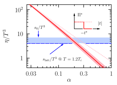
Figure 4 also shows that, despite the aforementioned uncertainties, $\eta_{{}_{\mathrm{LO}}}$ could be compatible with $\eta/s\mathrel{\hbox to0.0pt{\lower 1.99997pt\hbox{$\sim$}\hss}\raise 1.99997pt\hbox{$<$}}0.5$. The rigorous bound $s>4T^{3}$ of the interacting entropy for $T>1.2T_{c}$ is known from lattice calculations Giusti2017 . Thus the resummed LO viscosity may actually provide a prudent basis for extrapolation, rather than grossly overestimating $\eta/s$, it would actually give $\eta/s<1/(4\pi)$ for large enough $\alpha$. That brings us back to the central issue of coupling renormalisation at finite-$T$, i. e. what is $\alpha$?

3.2 Running coupling

For QCD there is no preferred value for $\alpha$ (such as $\alpha_{\rm em}=\frac{1}{137}$ in QED for all practical purposes). Loop corrections include both vacuum effects and (finite) thermal fluctuations, of which the latter survive the classical ‘$\hbar\to 0$’ limit. To then self-consistently define the running coupling, even at the LL level, one must retain the first term in (24). In Coulomb gauge, this is easily demonstrated because of the simple Ward identities already mentioned.

Typical loop integrals in quantum field theory give infinities which require renormalisation: connecting renormalised parameters with observables at the renormalisation scale. A textbook result ItzyksonZuber , handled through dimensional regularisation with the auxiliary scale $L$, isolates the divergent term

$$\Pi_{\mu\nu}\Big{|}_{T=0}=\alpha\beta_{0}\big{(}\,Q^{2}g_{\mu\nu}-Q_{\mu}Q_{\nu}\,\big{)}\Big{[}\ \frac{1}{\epsilon}+\log\frac{-Q^{2}}{L^{2}}\ \Big{]}\ ;\quad\epsilon\to 0\,.$$ (25)

Here $\beta_{0}=(33-2n_{\!f})/(12\pi)$ for QCD, where a positive value $\beta_{0}>0$ signals antiscreening of colour charges. In vacuum, the transverse and longitudinal projections coincide and are equal to $\Pi^{\rm vac}(Q)\equiv\,\alpha\beta_{0}[\epsilon^{-1}+\log(-Q^{2}/L^{2})]Q^{2}$  .

This brings us to the crux of our argument, which parallels the standard scenario at $T=0$ : Since the scale $L$ was auxiliary, we use it as the scale with which we fix parameters in the theory. Consider an experiment at the scale $\hat{t}=-L^{2}$, thus producing a finite value for $(\alpha^{-1}-\epsilon^{-1})$ which defines an effective coupling $\hat{\alpha}^{-1}$. (I.e. the renormalised coupling at the scale $\hat{t}$.) This is sufficient to make predictions at $Q^{2}\neq\hat{t}$ and leads directly to the 1-loop running coupling formula,

$$\alpha(Q^{2}) = \big{[}\beta_{0}\log(-Q^{2}/\Lambda^{2})\big{]}^{-1}\,,$$ (26)

where the scale $\Lambda$ is determined by $L$ and the accompanying $\hat{\alpha}$ . Dressing an internal propagator $D_{\mu\nu}$, leads to the renormalised amplitudes [for the replacement rule (23)]

$$\alpha\Delta(Q) \to \frac{\alpha}{Q^{2}-\big{(}\,\Pi^{\rm vac}+\widetilde{\Pi}\,\big{)}}\ =\ \Big{[}\ \frac{Q^{2}}{\alpha(Q^{2})}-4\pi T^{2}\,\phi(\omega,\mbox{\boldmath$q$})\ \Big{]}^{-1}\,.$$ (27)

For large enough $-Q^{2}$ (due to asymptotic freedom; the screening term is insignificant in the denominator), we recover the familiar result, e. g.  ${\cal M}^{\rm vac}\sim\alpha(t)/t$ for a $t$-channel process like Fig. 1. In this sense, the relevant scale in $\alpha(\cdot)$ is dictated by the process Cutler1978 . For $T>0$, the running coupling also applies to thermal screening $\widetilde{\Pi}(Q)\sim\alpha(Q^{2})T^{2}$, see Fig. 5. Screening is then a genuine ‘perturbation’ for $|t|^{1/2}\gg\Lambda$ because $\alpha$ is small, although (as mentioned) HTL propagators are no longer valid. Notwithstanding soft momenta $|Q^{2}|\simeq\Lambda^{2}$, where screening is crucial, the ratio $Q^{2}/\alpha(Q^{2})$ is then small by assumption. Thus where pQCD becomes dubious, the matrix element saturates at some finite value, rather than giving an obviously unphysical result. At ‘strong coupling’ the totally screened cross section actually leads to a minimum bound on $\eta$. On these grounds, an extrapolation of $\sigma_{\rm tr}$ using Eq. (27) may actually yield reasonable estimates, e. g. for $\eta$, since screening protects $|t|^{1/2}\to\Lambda$.

Figure 5: Example of a 1-loop contribution to the gluon self-energy. Regularising the vacuum contribution, cf. Eq. (25), we illustrate that the external momentum $t$ is the correct scale for the coupling in thermal mass $\widetilde{\Pi}(Q)\sim\alpha(t=Q^{2})T^{2}$ – not the typical loop momentum $Q_{T}\simeq 2\pi T$ often presumed.

Strictly speaking, the ‘right’ value of $\alpha(\cdot)$ should be established by calculating all ${\cal O}(\alpha)$ corrections. Evidently we have not done this. Instead we advocate resumming a subset of these: Those which come with large logarithms $\alpha(Q^{2})\log(Q^{2}/t)$, and can be eliminated by choosing $Q^{2}=t$. We cannot say whether the uncalculated corrections will be large or small (see discussion in Sec. 2), but it seems legitimate to ask what effect it has. Because it is based on adding vacuum corrections to the (already) minimal requirement for screening, we speculate that it is also important for extrapolating the LO result.

3.3 Treatment of ‘subleading’ terms

The dominant contribution to $\eta$ comes from terms in $d\sigma^{\rm tree}/dt$ that resemble (27), and also give the LL result in a parametric calculation. Having found large (but not unreasonable) sensitivity to the limited scope of the HTL functions (see Fig. 4), we can afford to make some simplifications in subleading terms.

That is the reason we have altogether dropped inelastic processes, which affect $\eta_{{}_{\mathrm{LO}}}$ by merely a few percent Arnold2003f . Similarly, the terms in $d\sigma^{\rm tree}/dt$ that do not need to be screened give a numerically minor contribution (screening is entirely omitted for them); see Fig. 6. To correctly incorporate screening into the sub-dominant and $s$-channel process would require dressing the individual amplitudes ${\cal M}_{i}$, rather than selectively mending the total cross section $d\sigma/dt\sim|\sum{\cal M}_{i}|^{2}$.

Figure 6: Relative contribution from subleading terms in $d\sigma^{\rm tree}/dt$, which do not require screening in Eq. (22) (hence no sensitivity to $t^{\star}$). Here $\delta\eta=\eta_{{}_{\mathrm{LO}}}-\bar{\eta}$ where $\bar{\eta}$ is without certain contributions (labelled by arrows) to $d\sigma^{\rm tree}/dt$. Then $\delta\eta/\eta_{{}_{\mathrm{LO}}}$ is a ‘fraction’ of the Red curve in Fig. 4. The $s$-channel contribution is negative, but small. A maximal coupling value is from (28).

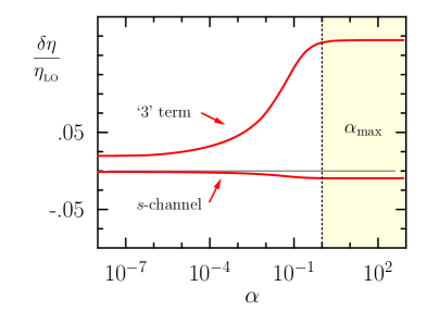
Hence we cannot preclude $|{\cal M}^{2}|<0$ in the numerical evaluation of ${\cal C}[\chi]$, but it seems to carry barely any influence on its value. (Figure 6 shows why; the offending terms are subleading.)

Equation (26) applies to the space-like exchanges in $d\sigma^{\rm tree}/dt$ that require thermal screening. Although it would be tempting to simply evaluate $\alpha(Q^{2})$ at the virtuality of the intermediate state $Q^{2}=\{s,t,u\}$, that would in any case not help for the inelastic scatterings. We motivated a running coupling only for the leading IR terms. For the rest, let us simply take $Q^{2}=(stu)^{1/3}$, and use the continuation of (26), as advocated in Shirkov1997a

$$\alpha_{\rm eff}(Q^{2}) = \frac{1}{\pi\beta_{0}}A\big{(}Q^{2}/\Lambda^{2}\big{)}\,,$$ (28)

where the (analytic) function $A$ is defined by

$$A(y)=\left\{\begin{array}[]{l}\displaystyle\frac{\pi}{\log(-y)}+\frac{\pi}{1+y}\\[11.38092pt] \displaystyle\frac{\pi}{2}-\arctan\Big{(}\,\frac{1}{\pi}\log\,y\,\Big{)}\end{array}\right.\quad\text{for}\ y\mathrel{\hbox to0.0pt{\lower 2.5pt\hbox{$>$}\hss}\raise 2.5pt\hbox{$<$}}0\,.$$

Despite intrinsic difficulties with QCD in the far infrared, perturbation theory can give semi-quantitative results Dokshitzer2002 . This model expression (28) has a ‘universal’ limiting value at $Q^{2}\to 0$, (from above or below), that imposes a maximal value $\alpha(\cdot)\leq\alpha_{\rm max}=1/\beta_{0}$. Numerically $\alpha_{\rm max}=\{1.1,1.3\}$ for $n_{\!f}=0$ and $3$ . and having larger values of $\alpha$ (i. e. from using the naïve one-loop formula with $\alpha_{\rm max}\mathrel{\hbox to0.0pt{\lower 1.99997pt\hbox{$\sim$}\hss}\raise 1.99997pt\hbox{$>$}}1$ imposed by hand) does not markedly change the results, see Fig. 6. The reason for this was already discussed around Eq. 27.

4 Results

Given then, is $\eta/T^{3}$ as a function of $T/\Lambda$ via the scales that go into $\alpha(\cdot)\,$. Figure 7 shows the resulting temperature dependence for $\eta_{{}_{\rm LO}}/T^{3}$, determined using Eq. 28 with an appropriate scale in the renormalised HTL propagators. [The details are in Sec. 3, and actual $Q^{2}$-values are intergration variables for (19)]. Also shown in Fig. 7 is the NLL result (4), with a running coupling $\alpha(Q_{T}^{2})$ where $Q_{T}=\xi\cdot 2\pi T$ for $\xi\in[\frac{1}{2},2]$. Evidently the two curves approach one another for $T\gg\Lambda$, still differing by a factor $\approx 2$ at $T/\Lambda=10^{3}$, for which the naïve coupling is $\alpha(Q_{T})=0.1\,$. Note in particular, that $\alpha(2\pi T_{c}/\Lambda)\approx 0.3$ – just about $\underline{\alpha}$ where (4) breaks down. Changing $\xi$ is akin to a trivial rescaling of $\Lambda$ (since only the ratio $Q_{T}/\Lambda$ is important for $\eta_{{}_{\rm NLL}}/T^{3}$), and thus merely shifts the corresponding curve in Fig. 7 to the left or right.

Figure 7: Temperature dependence of the viscosity in the quenched limit ($n_{\!f}=0$). The purple curves (solid, dashed and dotted) represents the NLL result for $\eta$ (see Fig. 2), and with a coupling at the thermal scale $Q_{T}=4\pi T$; dotted, $2\pi T$; solid and $\pi T$; dash-dotted. The solid (red) line, surrounded by a light band, is our 1-loop resummation scheme (see text for details) with a ‘canonical’ choice of screening only where $|t|<-t^{\star}\sim T^{2}$. The blue squares are the lattice results Giusti2017 and the arrow points to the Stefan-Boltzmann limit.

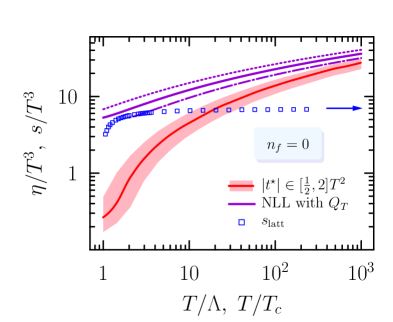
Plotting the interacting entropy $s(T)/T^{3}$, obtained now to high precision for $T\leq 300T_{c}$ Giusti2017 , on the same axis illustrates $\eta=s$ only at moderately large temperatures $T\simeq 20T_{c}$ (assuming $\Lambda=T_{c}$). The entropy (being a measure of the available degrees of freedom) increases rapidly at at the transition, and is within 5% of the Stefan-Boltzmann limit after $T\mathrel{\hbox to0.0pt{\lower 1.99997pt\hbox{$\sim$}\hss}\raise 1.99997pt\hbox{$>$}}2T_{c}$. The shear viscosity (divided by $T^{3}$) increases more gradually above $T_{c}$, due to asymptotic freedom. [The mean free path becomes small, due to $\lambda\propto T^{-1}$, but but also depends weakly on $\alpha$, see (2).] However for physically relevant temperatures, just above the crossover (say $T<4T_{c}$), the renormalised prediction is an order of magnitude smaller than the naïve application of the NLL result. And while there is no guarantee that pQCD (or indeed kinetic theory) is applicable here, it is just what one would expect from a reasonable extension of the curve at $T\simeq 20T_{c}$ (where $\eta=s$). We shall speculate on this extrapolation after first presenting the subsequent ratio $\eta/s$, for $T\mathrel{\hbox to0.0pt{\lower 1.99997pt\hbox{$\sim$}\hss}\raise 1.99997pt\hbox{$>$}}T_{c}$.

4.1 Estimation of $\eta$$/$$s$

The interacting entropy is now well established in the published lattice QCD data (available for $n_{\!f}=\{0,3\}$) Giusti2017 ; Bazavov2014f , and we shall use it to normalise our perturbative result for $\eta$. Adjusting the quantity $\ell=\Lambda/T_{c}$ in the ratio

$$\eta\left(T/\mbox{\boldmath$($}\ell\,T_{c}\mbox{\boldmath$)$}\right)\big{/}s_{\rm latt}\left(T/T_{c}\right)\,,$$

overlays the units for the abscissa in in Fig. 7.

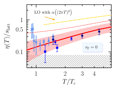
For $n_{\!f}=0$, there are several evaluations of $\eta_{\rm\,latt}$ Meyer2007f ; Meyer2009e ; Mages2015 ; Astrakhantsev2017 . (Caveats, mentioned in Sec. 1 , should be reiterated here: A dynamical quantity is difficult to extract by means of equilibrium lattice gauge theory.) Nevertheless, if we confront the LO calculations with $\eta_{\rm\,latt}$ at the simulated temperatures and use $\ell=1/1.26$ Borsanyi2012e , we find that $\eta_{{}_{\mathrm{LO}}}(T)$ is quite compatible. Figure 8 indeed reveals that our calculation corroborates the lattice data, and can explain $\eta/s\approx 0.2$ at $T<2T_{c}\,$. Modifying the self energy in the screened propagators via $t^{\star}\in-[\frac{1}{2},2]T^{2}$ gives a family of curves that cover the estimated uncertainty from $\eta_{\rm\,latt}$. Setting $t^{\star}/T^{2}=-\infty$, i. e. using HTL functions for all $\omega$ and $|\mbox{\boldmath$q$}|$, gives $\eta$ about a factor of two larger. This is to be expected, based on the similar sensitivity for the toy model in Sec. 2 [see eq. (7)].

Using the coupling at an argument $Q_{T}=2\pi T$ would instead yield $\eta_{{}_{\mathrm{LO}}}\mbox{\boldmath$($}\alpha(Q_{T})\mbox{\boldmath$)$}/s\mathrel{\hbox to0.0pt{\lower 1.99997pt\hbox{$\sim$}\hss}\raise 1.99997pt\hbox{$>$}}0.7$, which still does not explain $\eta/s<0.5$. Adjusting (via $\xi$) the scale $Q_{T}=\xi\cdot 2\pi T$, to have $\eta_{{}_{\mathrm{LO}}}(\alpha)/s_{\rm latt}<0.5$ at $T=1.2T_{c}$ would require $\alpha\mathrel{\hbox to0.0pt{\lower 1.99997pt\hbox{$\sim$}\hss}\raise 1.99997pt\hbox{$>$}}0.4$ (see Fig. 4). It then seems difficult to justify the resulting $\xi\mathrel{\hbox to0.0pt{\lower 1.99997pt\hbox{$\sim$}\hss}\raise 1.99997pt\hbox{$<$}}0.3\Lambda/T_{c}$ from using (28). Moreover, the corresponding curve would give the wrong slope for $\eta/s$ as a function of $T$. Confinement sets in for $T<T_{c}\,$, where the unmistakable increase in $\eta/s$ is due to both a reduced entropy and larger viscosity: $\eta_{{}_{\rm glueball}}\sim(\Lambda/T)^{5/2}$ Hosoya1985a .

Figure 8: A renormalised prediction for $\eta/s$, as a function of $T/T_{c}$, in pure gauge QCD (assuming $T_{c}/\Lambda=1.26$). The lattice data are from Refs. Meyer2007f ; $\Box$, Meyer2009e ; $\triangle$, Mages2015 ; $\circ$ and Astrakhantsev2017 ; $\times$ . The dashed curve (orange) is the LO result from Arnold2003f , with a running coupling at the ‘hard’ thermal scale $Q_{T}=2\pi T$. Hatching indicates the region below the conjectured lower limit $1/(4\pi)$.

All our discussion trivially extends to the physical case, $n_{\!f}=3$, for which it ought to viewed in the context of RHIC and LHC programmes. There it has been established that the experimental data cannot be reproduced with a value $\eta/s>0.5$, by viscous hydrodynamic simulations Teaney2003a . $\eta/s$ is one input to these codes, whose value is tuned to cover the hadronic and QGP phase of the evolution near $T_{c}\,$. Studies first sought a feasible range for $\eta/s$ (to reproduce experiments):

Ref. Aamodt2011 & Adare2011 Luzum2008a Song2011e Gavin2006a

$$\frac{\eta}{s}\mathrel{\hbox to0.0pt{\lower 2.5pt\hbox{$<$}\hss}\raise 2.5pt\hbox{$>$}}$$

(30)

Recently, attempts have been made to constrain the temperature dependence of $\eta/s$, which is expected to be minimal at the crossover temperature Niemi2015qia ; Denicol2016 ; Bernhard2016 . These approaches are capable of eliminating certain models for $\eta(T)$; which also depends on $T<T_{c}$ (the hadronic phase of evolution). Simple parametrisations of $\eta/s$ are linear in $T$ with different slopes for $T\mathrel{\hbox to0.0pt{\lower 1.99997pt\hbox{$\sim$}\hss}\raise 1.99997pt\hbox{$>$}}\underline{T}$ (where $\eta/s$ is minimal at $\underline{T}\approx T_{c}\,$). Exploring minimal values from (30) offers some restrictions on the two slopes – although it remains difficult to discern the behaviour for $T>\underline{T}$ .

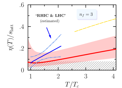
In Fig. 9 we show the viscosity to entropy density in the physical case, where we have set $\ell=1/0.48$ Aoki2009n . Our results are on the lower end of the parametrisations explored in hydrodynamics and predicts a milder increase with $T/T_{c}\,$. Apparently there is hardly any difference with the quenched results; the increased interaction rate is compensated by the density. There does seems to be more sensitivity to the HTL restriction from $t^{\star}$, which brings a factor $\approx 2$ uncertainty. For $T<3T_{c}$, it seems quite possible to violate the lower bound $1/(4\pi)$ – or not, depending on $t^{\star}$. As speculation, the smooth crossover in $s(T)$ (compared to $n_{\!f}=0$) may cause the minimum in $\eta/s$ to be shifted slightly; $\underline{T}\approx 1.5\,T_{c}$. (The fact that $s_{\rm latt}$ deviates from $s_{0}$ by 30% at $T=2T_{c}$ may indicate a change in quasiparticle structure already, which we assumed not the case for $\eta$.)

The ratio of the LO viscosity with $\alpha(Q_{T}^{2})$ versus our results is at the factor-of-2 level (for $T=4T_{c}$, see Fig. 9). So extrapolating the fixed-coupling results with $Q_{T}$ down to $T\sim 1.5T_{c}$, would give $\eta/s\approx 0.3$ (by eye) which is possible. However, the renormalised viscosity reaches this value already at $T\approx 5T_{c}$.

Figure 9: The normalised viscosity for $n_{\!f}=3$ flavours as a function of $T/T_{c}$ (here $\Lambda/T_{c}=2.1$ Aoki2009n  ). Our estimate for the sensitivity to higher order terms gives the band around the solid red curve (see Fig. 4). Blue curves illustrate the ‘most likely’ dependence from a Bayesian analysis using hydrodynamical simulations Bernhard2016 . (Mean; solid blue and 95%-confidence; dash-dots.) Hatching indicates $\eta/s\leq 1/(4\pi)$.

4.2 Kinetic Theory

We now pause to confront the question of whether kinetic theory is applicable in such a ‘strong coupling’ regime. At asymptotically high $T$, there is a clear ordering between the inter-particle distance $\bar{r}\sim T^{-1}$, the Debye screening length $m^{-1}_{D}\sim(\sqrt{\alpha}\,T)^{-1}$ and the (large or small-angle scattering) mean free path $\lambda\sim(\alpha^{j}\,T)^{-1}$ where $j=\{1,2\}$ Arnold2003a . So

$$\lambda\gg m_{D}^{-1}\gg\bar{r}$$

and it is permissible to neglect multi-particle correlations and treat the individual binary collisions as instantaneous. But the scales become comparable for achievable temperatures $T\approx T_{c}\,$.

For example; the Debye mass (computable on the lattice for $n_{\!f}=0$) is largest when $T=1.2T_{c}$ but still satisfies $m_{D}^{-1}\geq\frac{1}{3}T^{-1}$ Peshier2006 . The interparticle distance $\bar{r}\approx\frac{1}{2}n^{-1/3}$ follows from the number density $n=(16+\frac{21}{2}n_{\!f})\frac{\zeta(3)}{\pi^{2}}T^{3}$. Hence the effective range of interactions is approximately equal to $\bar{r}$, which puts the physical picture at its limit but does not clearly invalidate it. Kinetic theory cannot be right at $T_{c}\,$, and thus we rather want to know where it actually breaks down.

Until now we have simply used the transport equation (8) as a starting point, and (with motivation) applied it where $\lambda$ may not be large (i. e. strong coupling). To justify this idea a posteriori, we show that the mean free path $\lambda$ comes to the order the inter-particle distance $\bar{r}$ at a only few times $T_{c}\,$. To define $\lambda$, we shall appeal to the relaxation approximation ${\cal C}[f_{1}]=-\delta f_{1}/\lambda$ in the Boltzmann equation (8). After linearising, $\lambda(E_{1})$ is expressed in terms of the collision operator,

$$\lambda^{-1}(E_{1})=\frac{1}{6E_{1}}\int d\Gamma\,\frac{tu}{s^{2}}|{\cal M}|^{2}\frac{f_{2}\bar{f}_{3}\bar{f}_{4}}{\bar{f}_{1}}\,.$$ (31)

The transport factor $tu/s^{2}=\frac{1}{4}(1-\cos^{2}\theta)$ comes from $\hat{p}_{1}^{i}\hat{p}_{1}^{j}\Delta^{ij}[\chi]\big{|}_{\chi=p^{2}}$ evaluated in the centre of momentum frame ($\theta$ is the scattering angle). We may then calculate (31) with the screened QCD matrix elements ${\cal M}$, and using the running coupling as put forward in Sec. 3.2. Figure 10 shows the resulting $\lambda(E)$ in units of $\bar{r}$, at $T=\{5T_{c},10T_{c}\}$. (The variation from modifying $t^{\star}$ from Sec. 3.1 is on par with a factor of 2 in temperature.)

Figure 10: Mean free path $\lambda\,$, for a gluon of energy $E\,$, in units of the mean interparticle distance $\bar{r}\,$. Two temperatures are shown (for $\ell=1/1.26$ as in Fig. 8).

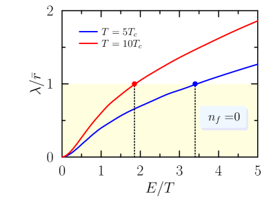
What fraction of particles is able to deliver its momentum across a path length $\lambda\geq\bar{r}$? If $\lambda=\bar{r}$ at $E\to E^{\star}$ then this fraction is $\int_{E^{\star}}^{\infty}dE\,E^{2}f(E)\big{/}(2\pi^{2}n)\,$. For the two temperatures shown in Fig. 10, we find that $70\%$ ($T=10T_{c}$) and $40\%$ ($T=5T_{c}$) particles meet this (albeit slightly arbitrary) requirement. Note that $T=5T_{c}$ is roughly the highest temperature used in lattice calculations of $\eta$ (see Fig. 8). Using $\bar{r}$ to qualify kinetic theory is not a rigorous judgement, but it at least demonstrates that we are at its limit for relevant temperatures $T\to T_{c}\,$.

For $n_{\!f}=3$, quarks and gluons will have different mean free paths. Because of the group factors in their interaction rate, $\lambda_{g}<\lambda_{q}\,$. Unfortunately there are large uncertainties coming from $t^{\star}$ in (31), hence we do not show a plot like Fig. 10. But is seems that $\lambda_{g}\mathrel{\hbox to0.0pt{\lower 1.99997pt\hbox{$\sim$}\hss}\raise 1.99997pt\hbox{$<$}}\bar{r}\mathrel{\hbox to0.0pt{\lower 1.99997pt\hbox{$\sim$}\hss}\raise 1.99997pt\hbox{$<$}}\lambda_{q}$ for the bulk of particles at a few times $T_{c}\,$.

5 Summary

In this paper we refute a widespread paradigm: That the inferred ratio of shear viscosity to entropy density of the QGP, $\eta/s\mathrel{\hbox to0.0pt{\lower 1.99997pt\hbox{$\sim$}\hss}\raise 1.99997pt\hbox{$<$}}0.5$ near the deconfinement temperature $T_{c}$, is a genuinely non-perturbative effect. Contrary to this view, we find that the LO weak coupling result of Ref. Arnold2003f can explain why $\eta$ is so low. Our main result is a new estimate for the temperature dependence of $\eta/s$, see Figs. 8 and 9.

We addressed two problems with many existing estimates from perturbation theory:

1. Logarithmic accuracy is appropriate only in scenarios where the coupling may be regarded as (asymptotically) weak. The increase of $\eta_{{}_{\rm NLL}}(\alpha)$ for $\alpha>\alpha^{\star}$ is unphysical: we expect that the viscosity to decrease with the coupling strength.

2. A common procedure in using a fixed coupling result, is to choose the value of $\alpha$ as the running coupling $\alpha(Q^{2})$ at, or near, the lowest Matsubara energy. In fact, a scale-dependent coupling and the calculation scheme of LO approximations are closely related: both emerge from/take into account loop corrections to tree level-amplitudes.

Together, these improvements enable us to meaningfully extrapolate $\eta(T)$ near the QGP phase transition, provided that binary scatterings form the principal source of energy and momentum variation.

To see how the running may affect a coefficient like $\eta$, consider our earlier formula (2) for the transport cross section. Using (26) in (2) to LL accuracy, we find

$$\sigma_{\rm tr}(s)\sim\frac{1}{s}\int_{-s}^{-\mu^{2}}dt\,|t|\,\frac{\alpha(t)^{2}}{t^{2}}\ =\ \frac{1}{s}\alpha(\mu^{2})\alpha(s)\log\Big{(}\,\frac{s}{\mu^{2}}\,\Big{)}\,.$$ (32)

While the overall structure is unchanged, cf. (3), a substitution $\alpha^{2}\to\alpha(\text{\sl hard})\alpha(\text{\sl soft})$ in going from (4) to (32) reflects the relative importance of different scales. Soft interactions are more probable due to an overall $\alpha(t)^{2}$ in $d\sigma/dt$, but are also more screened by $\mu^{2}\sim\alpha(t)T^{2}$.

Resumming the vacuum self-energy $\Pi^{\rm vac}$ in (23) is ‘optional’, only thermal corrections must be taken into account (running in $\alpha$ is formally higher order). However, we may incorporate them so that vacuum and thermal parts are treated on an equal footing. And if we do, the benefit is to specify $\alpha$ (even at the LL level). In pursuing this line of reasoning, we have found that the scales in the running coupling could have a substantial effect on $\eta$.

Appendix A $P(s)$ distribution

A valuable clue as to the role of the ‘hard’ scale $s\sim T^{2}$, appearing in Eq. (5), is provided by the thermal weight $P[\chi]$, emerging from (19), whose properties we now explore.

Firstly, the condition for normalisation, i. e. $\int dsP(s)=2b$, is convenient for (6) but should be set by $\chi$. After using symmetry in the integration variables $p_{1,2}$ of (20), we may complete all but one integral to find (for notational convenience we put $T\to 1$ here)

$$\int dsP(s) = \frac{2}{3}(2\pi)^{-2}\int_{0}^{\infty}dpf\bar{f}\Big{[}\,\chi^{2}+\frac{p^{2}}{6}(\chi^{\prime})^{2}\,\Big{]}\,.$$

Requiring that this equals $2b$ imposes a restriction on the function $\chi$, that needs to be satisfied in addition to the constraint (21). Taken together, they imply $\chi$ must satisfy

$$\chi^{\prime\prime}+\Big{(}\,\frac{2}{p}-1-2f\,\Big{)}\chi^{\prime}-\frac{6}{p^{2}}\chi+Ap = 0\,.$$ (33)

$A$ is a Lagrange multiplier to set the norm of $\chi$ (it cannot be zero). This relation was also found in Ref. Heiselberg1994b in a different manner, directly evaluating (17) to LL accuracy. Because the solution to the Boltzmann equation $f_{\star}(p)=f[1+\chi\bar{f}(\hat{p}_{i}\hat{p}_{j}-\frac{1}{3}\delta_{ij})\nabla_{i}u_{j}]$ is positive and integrable, the function $\chi$ cannot grow exponentially fast. Suppose that $\chi(p)$ is normalised, in such a way that $\chi\to p^{\nu}$ for large $p$. Substituting into (33) with $f\approx 0$ gives $\nu=2$ and $A=2$. (Rescaling the asymptotic behaviour by some constant will just change $A$ by the same factor.)

$$\chi(p) \sim p^{2}+O(p)\,;\quad p\gg T\,.$$ (34)

In Ref. Baym1990 , the optimal solution to (18) of the same ‘single power’ form for all $p$ gave $\nu\approx 2.104$ .

For small arguments, $f(p)\simeq\frac{1}{p}-\frac{1}{2}+\frac{1}{12}p+\ldots$ in (33) and the first two terms in brackets thus cancel. The resulting asymptotic solution (contrary to the claim of Heiselberg1994b ) is

$$\chi(p) \sim p^{3}\Big{(}\,\bar{c}-\frac{2}{5}\log p\,\Big{)}+{\cal O}(p^{5})\,;\quad p\ll T\,,$$ (35)

with $\bar{c}\approx 0.62$ (this integration constant is set by (34), for which we have only a numerical value). Knowing the precise solution $\chi^{\star}$ to (33) only improves the estimate for $\eta$ in (19) by about $0.5$%. The large-$p$ behaviour $\chi\sim p^{2}$ turns out to be more important than (35), which is to be expected for a transport quantity. We thus explore below, the function $P[\chi](s)$ at the approximate solution $\chi\to p^{2}$.

Figure 11: The function $\chi/p^{2}$ as determined by Eq. (33). Also shown is the limit $\chi\sim p^{3}\log 1/p$ for $p\ll T$ (purple dotted line). $\chi\approx p^{2}$ appears to be an excellent approximation for $p\mathrel{\hbox to0.0pt{\lower 1.99997pt\hbox{$\sim$}\hss}\raise 1.99997pt\hbox{$>$}}T$.

Single-function Ansatz

For a given collisional parameter $s$, using (20) with $\chi(p)=p^{2}$, we define

$${P}(s) = \frac{1}{(2\pi)^{4}}\int dE_{1}dE_{1}\,f_{1}\bar{f}_{1}f_{2}\bar{f}_{2}\big{[}\,\frac{16}{3}E_{1}E_{2}\left(E_{1}-E_{2}\right)^{2}+\frac{2}{3}s\left(E_{1}^{2}+E_{2}^{2}+4E_{1}E_{2}\right)+s^{2}\,\big{]}\,.$$

(36)

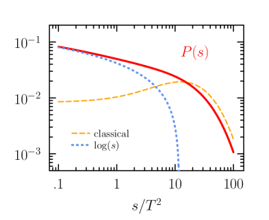
The integrals are over positive energies such that $E_{1}E_{2}\geq s/4$ . We do not have a simple closed form expression for $P(s)$ beyond a 1-dimensional integral over polylog functions, but we can state its large/small-$s$ behaviour

For large $s$, the thermal distributions can be replaced by classical Maxwell-Boltzmann distributions, i. e. $f_{1}\to\exp(-E_{1})$. We then obtain

$$P_{\rm cl.}(s) = \frac{s}{15\cdot 2^{12}\cdot\pi^{4}}\big{[}\,(40+3s)\sqrt{s}K_{3}\big{(}\sqrt{s}\big{)}-6sK_{4}\big{(}\sqrt{s}\big{)}\,\big{]}\,,$$

where $K_{3,4}$ are modified Bessel functions of the second kind.

The first few terms in an asymptotic series for $P(s)$ is given by

$$P(s) \sim \frac{32}{27}\,\Big{\{}\,54\zeta^{\prime}(3)-\pi^{4}+18\big{(}\,10-3\gamma-3\log\frac{s}{4}\,\big{)}\Big{\}}$$

$$\ +\frac{2s}{9}\,\Big{\{}\,66-12\gamma^{2}+\pi^{2}-54\log\frac{s}{4}+6\log^{2}\frac{s}{4}-24\gamma_{1}\,\Big{\}}+{\cal O}(s^{3})\,,$$

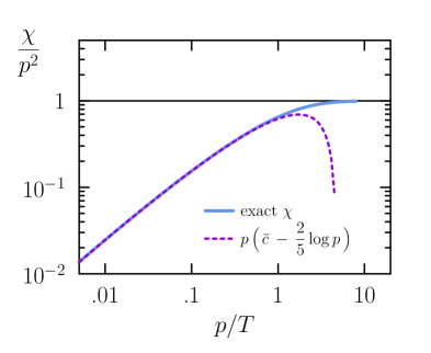
where $\gamma_{1}$ is the first Stieltjies constant (the Euler-Mascheroni constant $\gamma$ is $\gamma_{0}$). The qualitative feature we needed for the argument in Sec. 2 is indeed confirmed; $P(0)\neq 0$ (see Fig. 12), in fact there is an (integrable) log-divergence at $s\to 0$ .

The ‘moments’ $M_{n}=\int_{0}^{\infty}ds\,s^{n}P(s)$, are explicitly

$$M_{n} = \frac{4^{1+n}}{3\pi^{4}}\Gamma(n+1)\Gamma(n+4)$$

$$\qquad\times\Big{[}\zeta(n+4)\zeta(n+2)(n+4)(5+3n)+\zeta(n+3)^{2}n(7+3n)\Big{]}\,.$$

These moments grow extremely rapidly; $\log M_{n}\sim n\log n!$ as $n\to\infty$ . Once rescaled, $P(s)/M_{0}$ can be interpreted as a (normalised) probability distribution which then gives

$$\left<s\right>=M_{1}/M_{0}\simeq 27.7T^{2}\,,$$ (38)

$$\left<\log(s)\right>=\partial_{\epsilon}M_{\epsilon}/M_{0}\big{|}_{\epsilon\to 0}\simeq 0.381\,,$$ (39)

required to specify the parameter $\kappa$ for the effective model in Section 2.1 .

The general formula for the moments (A) allows for analytic continuation to complex $n$, inheriting properties from the $\Gamma$- and $\zeta$-functions. Isolated poles occur at $n=-1$ (double), $n=-2$ (triple) and double poles for all $n\leq-4$. This reaffirms the fact that ‘negative’ moments are divergent.

Figure 12: The (normalised) probability, (36) divided by $M_{0}$ . The small-$s$ expansion is shown for comparison (dotted blue line), and implies that the slope of $P$ at $s=0$ is infinite. The counterpart function for classical Maxwell-Boltzmann particles is also shown (orange dashed line).

Appendix B Soft & hard contributions

Particle production rates and transport coefficients require kinematic integral convolutions with matrix elements. In a thermal setting, particle propagators are modified by their interaction with the medium, a feature already stressed in Sec. 2. The general form of this screening is a $T^{2}$ multiplied by a dimensionless function of (separately) the momentum and frequency. The HTL approximation Braaten1990c affords an analytic representation depending only on $z=\omega/|\mbox{\boldmath$q$}|$. While usually derived under the assumption that both $\omega,|\mbox{\boldmath$q$}|\ll T$, the approximation is in fact valid for $|\omega^{2}-q^{2}|\mathrel{\hbox to0.0pt{\lower 1.99997pt\hbox{$\sim$}\hss}\raise 1.99997pt\hbox{$<$}}T^{2}$ Peshier1998 .

As mentioned in the body of the text (Sec. 3.1), we opt for a covariant separation of phase space with $t^{\star}$ as the cut-off parameter. The only difference with (7) comes from the HTL self-energies. Using the Born cross section where $-s<t<t^{\star}$, for the $t$-channel contribution of the scattering cross section gives a ‘trivial’ result. The essential contribution is

$$\sigma_{\rm tr}^{\rm hard}=\frac{1}{s}\int_{-s}^{t^{\star}}dt\,|t|\frac{\alpha^{2}}{t^{2}}=\frac{\alpha^{2}}{s}\log\frac{s}{|t^{\star}|}\,,$$ (40)

identical to (2) of course.

Screening is necessary for the complementary region, where $t^{\star}<t<0$. There is a further integration over the parameter $z\in[-1,+1]$ for time-like exchanges,

$$\sigma_{\rm tr}^{\rm soft}=\frac{1}{2s}\int_{-1}^{+1}dz\int_{t^{\star}}^{0}dt\frac{(-t)\alpha^{2}}{|t-\widetilde{\Pi}|^{2}}\,,$$ (41)

where $\widetilde{\Pi}=\widetilde{\Pi}_{L,T}(t,z)$ is the self energy. Since $|t^{\star}|\ll T^{2}$, the self-energy is independent of $t$ (so that HTL functions apply). This expression, when combined with the complementary region $t<t^{\star}$, produces no residual dependence on $t^{\star}$ (for weak coupling). In other words, it tells us at which point the HTL dressing is to be replaced by tree level functions. The expression in Eq. (41) was determined numerically, or in limiting cases. However it is possible to find the large-$|t^{\star}|$ contribution analytically in general. Keeping only relevant terms,

$$\int dt\frac{(-t)}{|t-\Pi|^{2}} = \int\frac{dt}{\mathrm{Im}\,\Pi}\mathrm{Im}\,\frac{\Pi}{t-\Pi}=\frac{1}{\mathrm{Im}\,\Pi}\mathrm{Im}\,\Big{[}\,\Pi\log\frac{|t^{\star}|+\Pi}{\Pi}\,\Big{]}\,.$$

Making use of the fact that $|t^{\star}|\gg|\Pi(z)|\sim\alpha T^{2}$ for weak coupling. To extract the leading cut-off dependence, up to ${\cal O}(m_{D}^{2}/t^{\star})$, we re-express the logarithms by

$$\log\frac{|t^{\star}|}{\Pi} = \log\frac{|t^{\star}|}{m_{D}^{2}}+\log\frac{m_{D}^{2}}{\Pi}\,,$$

where $m_{D}^{2}=4\pi\alpha T^{2}$ is the LO Debye mass (for $n_{\!f}=0$). The familiar log-structure emerges when $|t^{\star}|\rightarrow\infty$, plus a constant next to the logarithm,

$$\sigma_{\rm tr}^{\rm soft}=\frac{\alpha^{2}}{s}\Big{(}\log\frac{|t^{\star}|}{m_{D}^{2}}-\int_{0}^{1}dz\frac{1}{\mathrm{Im}\,\phi}\mathrm{Im}\,\!\big{[}\,\phi\log\phi\,\big{]}\Big{)}\,,$$ (42)

in terms of the function $\phi(z)=\Pi/m_{D}^{2}$, which is order of unity. We have used $\phi(z)^{*}=\phi(-z)$, to replace the original $z$-integral by one from $z=0$ to $1$. A contour in the complex $\phi$-plane, parametrised by $z$, is traced out with endpoints at $\phi(0)$ and $\phi(1)$, see Fig. 13.

Figure 13: The transport cross section takes into account screening via the function $\phi$ (which has real and complex parts), thus tracing a curve in the complex plane with $z$ as the parameter.

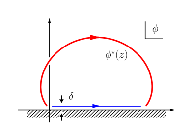
Formally, $\sigma_{\rm tr}^{\rm hard}+\sigma_{\rm tr}^{\rm soft}$ to NLL accuracy is then independent of $t^{\star}$, which cancels. I.e. $\sigma_{\rm tr}^{\rm NLL}=\frac{1}{s}\alpha^{2}[\log(s/m_{D}^{2})-\widetilde{c}\,]$, with $\widetilde{c}$ defined by the integral in (42). Relative errors in (42) are supressed by $m_{D}^{2}/|t^{\star}|\sim\alpha$ and amounts to a residual dependence on $t^{\star}$.

Equation (42) is directly applicable to the calculation for the transport cross section. In the quenched case, one needs the screened matrix element from $gg\rightarrow gg$ interactions. Take only the $t$- and $u$-channel from (22) with (23), one finds

$$\frac{d\sigma}{dt}\Big{|}_{t>t^{\star}} = \frac{\alpha^{2}}{3}\Big{[}\ \frac{1}{|t-\widetilde{\Pi}_{L}(z)|^{2}}+\frac{1/2}{|t-\widetilde{\Pi}_{T}(z)|^{2}}\ \Big{]}\,,$$ (43)

for $|t|\ll T^{2}$, and omitting all unnecessary prefactors. There are two terms of the type discussed in (41), where screening is accounted for by HTL gluon self energies, viz.

$$\phi_{L}(z) = (1-z^{2})\Big{(}\,1-\tfrac{1}{2}z\log\frac{z+1}{z-1}\,\Big{)}\,,$$

$$\phi_{T}(z) = \Big{(}\,\tfrac{1}{2}z^{2}+\tfrac{1}{4}z(1-z^{2})\log\frac{z+1}{z-1}\,\Big{)}\,.$$

Since $|z|<1$, the logarithms are complex, with values taken on the principal branch.

One has the freedom to deform this contour to a simple one (just above the real axis), say $\phi=\gamma+i\delta$ and examine the limit $\delta\to 0$. This dramatically simplifies the integrand appearing in Eq. (42);

$$\mathrm{Im}\,\Big{[}\,\frac{\phi\log\phi}{\delta}\,\Big{]}=\log\Big{(}\sqrt{\gamma^{2}+\delta^{2}}\,\Big{)}+\frac{\gamma}{\delta}\arg(\gamma+i\delta)\stackrel{{\scriptstyle\delta\to 0}}{{\simeq}}\log|\gamma|+1\,.$$ (44)

In the small-$|t|$ limit of (43), we can evaluate the transport cross section as follows. Deform the contour, see Fig. 13, to find that (for example) the longitudinal propagator gives a constant in (42),

$$\int_{0}^{1}d|\phi_{L}|\big{(}\,\log|\phi_{L}|+1\,\big{)}=|\phi_{L}(1)|\log|\phi_{L}(1)|-|\phi_{L}(0)|\log|\phi_{L}(0)|=0\,.$$ (45)

Only the transverse screening is non-zero, having $\phi_{T}(1)=\frac{1}{2}$, and ends up giving $\widetilde{c}=-\frac{1}{3}\log 2$ next to the LL in (42).

Combining the contribution from hard and soft regions given by (40) and (43) produces

$$\sigma_{\rm tr} = \frac{\alpha^{2}}{s}\Big{(}\,\log\frac{s}{m_{D}^{2}}-\tfrac{1}{3}\log 2\,\Big{)}\,.$$

This demonstrates the Braaten-Yuan (BY) method Braaten1991d , and confirms an earlier numerical result of Heiselberg in Eq. (B7) Heiselberg1994b . If we had used this result to match $\mu^{2}=\kappa\cdot m_{D}^{2}$ in the simple model (5), we would have found $\kappa=2^{1/3}/e\approx 0.46$ [this differs from the value $\kappa\approx 0.62$ obtained via (4), due to the omission of inelastic proccess, the gluon 4-vertex and $s$-channel diagrams in ${\cal M}$]. Incidently, this technique is applicable for calculating the photon rate and proves a result in Kapusta1991 previously known only numerically. Formally, $\sigma_{\rm tr}$ is then independent of $t^{\star}$ in the BY scheme resting on the assumption that $m_{D}^{2}\ll-t\ll s\sim T^{2}$. Residual dependence on $t^{\star}$ in (43) for subleading errors that are $\sim\Pi/|t^{\star}|$ and in (40) they are $\sim|t^{\star}|/s$.

Let us end with a comment on the finite radius of convergence for $\sigma_{\rm tr}$. In Sec. 2.1 we found that it was simply the ‘mass’ $\mu^{2}$ – here it will instead be given by the minimum of $|\Pi(z)|$. That is zero for HTL functions, but in general may be related to the QCD ‘magnetic’ mass. This speculation is well beyond our present scope.

Appendix C Two-body phase space

The collisional operator (8) expresses the rate of binary encounters, integrated over partner momenta $\mbox{\boldmath$p$}_{2}$, $\mbox{\boldmath$p$}_{3}$ and $\mbox{\boldmath$p$}_{4}$. For a given function $g\big{(}\{\mbox{\boldmath$p$}_{i}\}\big{)}$ which depends on the participant momenta, we evaluate the phase space integral, $\int d\Gamma\cdot g$. One of the integrals may be completed using energy-momentum conservation; we choose the $p_{4}$-integral,

$$\int_{4}\frac{g}{2E_{4}} = 2\pi\delta(\underline{K}_{4}^{2})\theta(\underline{E}_{4})\ \underline{g}\,.$$ (46)

Here the underline indicates a dependence on the fixed 4-momentum $\underline{K}_{4}=P_{1}+P_{2}-P_{3}$. For instance, $\underline{f}_{4}$ depends on the energy $\underline{E}_{4}=E_{1}+E_{2}-E_{3}$. It will turn out that the on-shell constraint $\underline{P}_{4}^{2}=0$, expressed by the $\delta$-function in (46), implies already $\underline{E}_{4}\geq 0$, making the factor of $\theta(\underline{E}_{4})$ redundant in (46). The remaining fivefold integral is further reduced as follows Peigne2008 . We align the $z$-axis with $\mbox{\boldmath$p$}_{1}$ and orient the $zy$-plane to contain $\mbox{\boldmath$p$}_{3}$ viz.

$$\mbox{\boldmath$p$}_{1} = E_{1}(0,0,1)\,,$$

$$\mbox{\boldmath$p$}_{2} = E_{2}(\sin\phi\sin\theta_{2},\cos\phi\sin\theta_{2},\cos\theta_{2})\,,$$

$$\mbox{\boldmath$p$}_{3} = E_{3}(0,\sin\theta_{3},\cos\theta_{3})\,.$$ (47)

The argument of the $\delta$-function in (46) depends on $\phi$ through

$$\underline{P}_{4}^{2} = 2(P_{1}P_{2}-P_{1}P_{3}-P_{2}P_{3})$$

$$= s+t-2P_{2}P_{3}\,.$$

Thus, using (47) to simplify the outstanding 4-product, we have $\underline{P}_{4}^{2}=A+B\cos\phi$ where

$$A = s+t-2E_{2}E_{3}(1-\cos\theta_{2}\cos\theta_{3})\,,$$

$$B = 2E_{2}E_{3}\sin\theta_{1}\sin\theta_{3}\,.$$ (48)

Emphasising the azimuthal dependence in $g=g(\phi)$, the $\phi$-integral is elementary

$$\int_{0}^{2\pi}d\phi\ \delta\left(\underline{P}_{4}^{2}\right)\ g(\phi) = E_{1}\frac{\theta(h)}{\sqrt{h}}\sum_{\pm}g(\phi_{\pm})\,,$$

where $\phi_{\pm}=\pi\pm\arccos(A/B)$ and $h=E_{1}^{2}(B^{2}-A^{2})$ ($E_{1}$ is factored out for convenience). Next, we reformulate the remaining integration over $\cos\theta_{2,3}$ in terms $s$ and $t$, whose values are specified by $\mbox{\boldmath$p$}_{1},\mbox{\boldmath$p$}_{2}$ and $\mbox{\boldmath$p$}_{3}$:

$$s = 2E_{1}E_{2}(1-\cos\theta_{2})\,,$$

$$t = -2E_{1}E_{3}(1-\cos\theta_{3})\,,$$ (49)

with Jacobian $4E_{2}E_{4}\cdot E_{1}^{2}$. Using this, and (46), we arrive at

$$\int d\Gamma\cdot g(\cdots) = \frac{1}{16(2\pi)^{4}E_{1}}\int dsdt\ \int dE_{2}dE_{3}\frac{\theta(h)}{\sqrt{h}}\sum_{\pm}\underline{g}(\phi_{\pm})\,.$$ (50)

The function $h$ is quadratic in $E_{3}$, written as $h(E_{3})=aE_{3}^{2}+bE_{3}+c$ the coefficients are found from (48) and (50) to be

$$a = -s^{2}\,,$$

$$b = -2s(uE_{1}+tE_{2})\,,$$

$$c = -(uE_{1}-tE_{2})^{2}-stu\,.$$

Since $a<0$, $\theta\left(h\right)$ constrains the $E_{3}$-integration to the interval $[E_{3}^{-},E_{3}^{+}]$, where

$$E_{3}^{\pm} = \frac{-b\pm\sqrt{D}}{2a}\,.$$

Positivity of the discriminant $D=4s^{2}tu(4E_{1}E_{2}-s)$ summarises the 2-body phase space: $0\leq s\leq s_{\rm max}=4E_{1}E_{2}$ and $-s\leq t\leq 0$.

With the kinematic bounds fully specified, the factor $\theta(h)$ can indeed (as anticipated) be dropped in (50) to give

$$\int d\Gamma\cdot g = \frac{1}{(2\pi)^{3}E_{1}}\int dE_{2}\int_{0}^{s_{\rm max}}ds\int_{-s}^{0}dt\ \frac{1}{16\pi}{\cal I}(s,t,E_{1},E_{2})\,,$$ (51)

in terms of a function that parametrises the final $E_{3}$-integral:

$${\cal I}[g]=\int_{E_{3}^{-}}^{E_{3}^{+}}\frac{dE_{3}}{\sqrt{h(E_{3})}}\ \frac{1}{2}\sum_{\pm}\underline{g}(E_{3},\phi_{\pm})\,.$$ (52)

Up to this point, there have been no simplifying approximations. After using energy and momentum conservation as well as symmetry in one of the angles, we have reduced the original expression (46) to a four dimensional integration.

Small-$t$ approximation

Of interest to Sec. 2, is the behaviour of (51) assuming dominance of small angle scatterings. We now discuss in some more detail how to complete the $E_{3}$-integral of (51), keeping terms of relevant powers in $t$. For small $\omega=E_{1}-E_{3}$, it is reasonable to replace in $g(E_{3})$ the energy $E_{3}\to E_{1}$. However, for $-t\ll T^{2}$ it remains possible that both $|\omega|$ and $q$ are individually large.

The integrand (52) has nonzero support for $h(E_{3})>0$, which as $|t|\to 0$ becomes very narrow; $(E_{3}^{+}-E_{3}^{-})=\frac{2}{s}\sqrt{tu(s_{\rm max}-s)}$ with the central value

$$E_{3}^{\star} = E_{1}-\frac{t}{s}\big{(}E_{2}-E_{1}\big{)}\,.$$

Let us suppose that the integrand $g$ is largest for small-$t$ (or $u$), and accordingly expand $g(E_{3},\cdots)$ about $E_{3}^{\star}$ (i. e. if $-t\ll s$, then $E_{3}\simeq E_{1}$). We thus represent $g$ in powers of $(E_{3}-E_{3}^{\star})$, to be integrated in (52), leading us to

$${\cal I}[g]=\sum_{k=0}^{\infty}{\cal I}_{(k)}\frac{\partial^{k}g}{\partial E_{3}^{k}}\bigg{|}_{E_{3}=E_{3}^{\star}}\,,$$ (53)

where ${\cal I}_{(k)}={\cal I}[(E_{3}-E_{3}^{\star})^{k}]/(k!)$. Only the first few terms in (53) turn out to be relevant, namely

ℐ(k)πs 0π16Ds5,fragments fragmentsI𝑘fragments𝜋𝑠fragments 0fragments𝜋16𝐷superscript𝑠5\begin{tabular}[]{c||c|c|c}$k$&0&1&2\\ \hline\cr${\cal I}_{(k)}\ $&$\ \displaystyle\frac{\pi}{s}\ $&$\ \displaystyle 0\ $&$\ \displaystyle\frac{\pi}{16}\frac{D}{s^{5}}\ $\end{tabular}\,,

k012k012 (54)

for $k\geq 3$ we find ${\cal I}_{(k)}={\cal O}(D^{k/2})$, which is subleading for small-$t$ or $u$. If we let $g^{\prime}=\partial g/\partial E_{3}$, then the leading terms for a small-$t$ approximation may be written

$${\cal I}[g] \simeq \frac{\pi}{s}g(E_{3}^{\star})+\frac{\pi}{4s^{3}}tu\big{(}4E_{1}E_{2}-s\big{)}g^{\prime\prime}(E_{3}^{\star})$$ (55)

It will turn out (see below), basically because of the choice of tensor basis (11), that $g(E_{3}^{\star})\propto tu$ and therefore both terms above are ${\cal O}(tu/s^{2})$ . The pertinent transport weight, $|t|$ in (55), emerges from the peaked kinematics for $E_{3}\sim E_{1}$ as $t\to 0$ (or $E_{3}\sim E_{2}$ as $u\to 0$).

For the linearised collisional operator (16), the QCD matrix element is largest when $t$ or $u$ is small compared with $s$. Here the integrand is

$$g(\cdots)=|{\cal M}|^{2}f_{1}f_{2}\bar{f}_{3}\bar{f}_{4}\cdot\big{(}\Delta^{ij}[\chi]\big{)}^{2}\,,$$

which depends on the unknown function $\chi$. Because $E^{\star}_{3}\simeq E_{1}$, up to subleading corrections for $-t\ll s$, we can replace $f_{3}\to f_{1}$, which gives

$$\int d\Gamma\cdot g = \frac{f_{1}\bar{f}_{1}}{(2\pi)^{3}E_{1}}\int dE_{2}\,f_{2}\bar{f}_{2}\int ds\,s^{2}\int dt\frac{d\sigma}{dt}\,{\cal I}\mbox{\boldmath$[$}\,\big{(}\Delta^{ij}[\chi]\big{)}^{2}\,\mbox{\boldmath$]$}\,,$$ (56)

assuming that the cross section $d\sigma/dt=|{\cal M}|^{2}/(16\pi s^{2})$ is only a function of $s$ and $t$. $\chi$ represents the input to the functional ${\cal Q}[\chi]$, see Eq. (17), whose maximal value gives $\eta$. Hence

$${\cal I}=\frac{\pi|t|}{4s^{2}}\big{[}\,8s{\cal A}+\big{(}4E_{1}E_{2}-s\big{)}{\cal B}\,\big{]}\,,$$

where ${\cal A}$ and ${\cal B}$ were given in (20).

References

- (1) D. Teaney, The Effects of viscosity on spectra, elliptic flow, and HBT radii, Phys. Rev. C68 (2003) 034913, [nucl-th/0301099].
- (2) P. Danielewicz and M. Gyulassy, Dissipative Phenomena in Quark Gluon Plasmas, Phys.Rev. D31 (1985) 53–62.
- (3) P. Kovtun, D. T. Son and A. O. Starinets, Viscosity in strongly interacting quantum field theories from black hole physics, Phys. Rev. Lett. 94 (2005) 111601, [hep-th/0405231].
- (4) S. Caron-Huot, S. Jeon and G. D. Moore, Shear viscosity in weakly coupled N = 4 super Yang-Mills theory compared to QCD, Phys. Rev. Lett. 98 (2007) 172303, [hep-ph/0608062].
- (5) H. Niemi, K. J. Eskola and R. Paatelainen, Event-by-event fluctuations in a perturbative QCD + saturation + hydrodynamics model: Determining QCD matter shear viscosity in ultrarelativistic heavy-ion collisions, Phys. Rev. C93 (2016) 024907, [1505.02677].
- (6) G. Denicol, A. Monnai and B. Schenke, Moving forward to constrain the shear viscosity of QCD matter, Phys. Rev. Lett. 116 (2016) 212301, [1512.01538].
- (7) H. B. Meyer, A Calculation of the shear viscosity in SU(3) gluodynamics, Phys. Rev. D76 (2007) 101701, [0704.1801].
- (8) H. B. Meyer, Transport properties of the quark-gluon plasma from lattice QCD, Nucl. Phys. A830 (2009) 641C–648C, [0907.4095].
- (9) S. W. Mages, S. Borsányi, Z. Fodor, A. Schäfer and K. Szabó, Shear Viscosity from Lattice QCD, PoS LATTICE2014 (2015) 232.
- (10) N. Astrakhantsev, V. Braguta and A. Kotov, Temperature dependence of shear viscosity of SU(3)-gluodynamics within lattice simulation, EPJ Web Conf. 137 (2017) 07003.
- (11) F. Reif, Fundamentals of Statistical and Thermal Physics. McGraw Hill, 1964.
- (12) A. Hosoya and K. Kajantie, Transport Coefficients of QCD Matter, Nucl.Phys. B250 (1985) 666.
- (13) G. Baym, H. Monien, C. Pethick and D. Ravenhall, Transverse Interactions and Transport in Relativistic Quark - Gluon and Electromagnetic Plasmas, Phys.Rev.Lett. 64 (1990) 1867–1870.
- (14) H. Heiselberg, Viscosities of quark - gluon plasmas, Phys.Rev. D49 (1994) 4739–4750, [hep-ph/9401309].
- (15) P. B. Arnold, G. D. Moore and L. G. Yaffe, Transport coefficients in high temperature gauge theories. 1. Leading log results, JHEP 0011 (2000) 001, [hep-ph/0010177].
- (16) P. B. Arnold, G. D. Moore and L. G. Yaffe, Transport coefficients in high temperature gauge theories. 2. Beyond leading log, JHEP 0305 (2003) 051, [hep-ph/0302165].
- (17) P. B. Arnold, G. D. Moore and L. G. Yaffe, Effective kinetic theory for high temperature gauge theories, JHEP 01 (2003) 030, [hep-ph/0209353].
- (18) A. D. Linde, Infrared Problem in Thermodynamics of the Yang-Mills Gas, Phys. Lett. B96 (1980) 289–292.
- (19) C. Itzykson and J.-B. Zuber, Quantum Field Theory. Dover Publications, 2006.
- (20) G. Jackson and A. Peshier, Low-shear QCD plasma from perturbation theory, 1704.06284 and a related web page http://github.com/gw3g/runny-gauge.
- (21) A. Peshier, K. Schertler and M. H. Thoma, One loop selfenergies at finite temperature, Annals Phys. 266 (1998) 162–177, [hep-ph/9708434].
- (22) E. Braaten and T. C. Yuan, Calculation of screening in a hot plasma, Phys. Rev. Lett. 66 (1991) 2183–2186.
- (23) J. Blaizot, E. Iancu and A. Rebhan, Approximately selfconsistent resummations for the thermodynamics of the quark gluon plasma. 1. Entropy and density, Phys.Rev. D63 (2001) 065003, [hep-ph/0005003].
- (24) A. Grozin, Asymptotic freedom: History and interpretation, 0803.2589.
- (25) H. A. Weldon, Covariant calculations at finite temperature: The relativistic plasma, Phys.Rev. D26 (1982) 1394.
- (26) L. Giusti and M. Pepe, Equation of state of the SU(3) Yang-Mills theory: A precise determination from a moving frame, Phys. Lett. B769 (2017) 385–390, [1612.00265].
- (27) R. Cutler and D. W. Sivers, Quantum Chromodynamic Gluon Contributions to Large p(T) Reactions, Phys. Rev. D17 (1978) 196.
- (28) D. V. Shirkov and I. L. Solovtsov, Analytic model for the QCD running coupling with universal alpha-s (0) value, Phys. Rev. Lett. 79 (1997) 1209–1212, [hep-ph/9704333].
- (29) Y. Dokshitzer, QCD at moderately large distances, Nucl. Phys. A711 (2002) 11–18, [hep-ph/0510199].
- (30) HotQCD collaboration, A. Bazavov et al., Equation of state in ( 2+1 )-flavor QCD, Phys. Rev. D90 (2014) 094503, [1407.6387].
- (31) S. Borsanyi, G. Endrodi, Z. Fodor, S. D. Katz and K. K. Szabo, Precision SU(3) lattice thermodynamics for a large temperature range, JHEP 07 (2012) 056, [1204.6184].
- (32) ALICE collaboration, K. Aamodt et al., Higher harmonic anisotropic flow measurements of charged particles in Pb-Pb collisions at =2.76 TeV, Phys. Rev. Lett. 107 (2011) 032301, [1105.3865].
- (33) PHENIX collaboration, A. Adare et al., Heavy Quark Production in and Energy Loss and Flow of Heavy Quarks in Au+Au Collisions at GeV, Phys. Rev. C84 (2011) 044905, [1005.1627].
- (34) M. Luzum and P. Romatschke, Conformal Relativistic Viscous Hydrodynamics: Applications to RHIC results at s(NN)**(1/2) = 200-GeV, Phys. Rev. C78 (2008) 034915, [0804.4015].
- (35) H. Song, S. A. Bass, U. Heinz, T. Hirano and C. Shen, 200 A GeV Au+Au collisions serve a nearly perfect quark-gluon liquid, Phys. Rev. Lett. 106 (2011) 192301, [1011.2783].
- (36) S. Gavin and M. Abdel-Aziz, Measuring Shear Viscosity Using Transverse Momentum Correlations in Relativistic Nuclear Collisions, Phys. Rev. Lett. 97 (2006) 162302, [nucl-th/0606061].
- (37) J. E. Bernhard, J. S. Moreland, S. A. Bass, J. Liu and U. Heinz, Applying Bayesian parameter estimation to relativistic heavy-ion collisions: simultaneous characterization of the initial state and quark-gluon plasma medium, Phys. Rev. C94 (2016) 024907, [1605.03954].
- (38) PACS-CS collaboration, S. Aoki et al., Precise determination of the strong coupling constant in N(f) = 2+1 lattice QCD with the Schrodinger functional scheme, JHEP 10 (2009) 053, [0906.3906].
- (39) A. Peshier, Running coupling and screening in the (s)QGP, hep-ph/0601119.
- (40) A. Peshier, The QCD collisional energy loss revised, Phys.Rev.Lett. 97 (2006) 212301, [hep-ph/0605294].
- (41) E. Braaten and R. D. Pisarski, Soft Amplitudes in Hot Gauge Theories: A General Analysis, Nucl.Phys. B337 (1990) 569.
- (42) J. I. Kapusta, P. Lichard and D. Seibert, High-energy photons from quark - gluon plasma versus hot hadronic gas, Phys.Rev. D44 (1991) 2774–2788.
- (43) S. Peigne and A. Peshier, Collisional Energy Loss of a Fast Muon in a Hot QED Plasma, Phys.Rev. D77 (2008) 014015, [0710.1266].