Large NLO corrections in $t\bar{t}W^{\pm}$ and $t\bar{t}t\bar{t}$ hadroproduction from supposedly subleading EW contributions

Abstract

We calculate the complete-NLO predictions for $t\bar{t}W^{\pm}$ and $t\bar{t}t\bar{t}$ production in proton–proton collisions at 13 and 100 TeV. All the non-vanishing contributions of $\mathcal{O}(\alpha_{s}^{i}\alpha^{j})$ with $i+j=3,4$ for $t\bar{t}W^{\pm}$ and $i+j=4,5$ for $t\bar{t}t\bar{t}$ are evaluated without any approximation. For $t\bar{t}W^{\pm}$ we find that, due to the presence of $tW\to tW$ scattering, at 13(100) TeV the $\mathcal{O}(\alpha_{s}\alpha^{3})$ contribution is about 12(70)% of the LO, i.e., it is larger than the so-called NLO EW corrections (the $\mathcal{O}(\alpha_{s}^{2}\alpha^{2})$ terms) and has opposite sign. In the case of $t\bar{t}t\bar{t}$ production, large contributions from electroweak $tt\to tt$ scattering are already present at LO in the $\mathcal{O}(\alpha_{s}^{3}\alpha)$ and $\mathcal{O}(\alpha_{s}^{2}\alpha^{2})$ terms. For the same reason we find that both NLO terms of $\mathcal{O}(\alpha_{s}^{4}\alpha)$, i.e., the NLO EW corrections, and $\mathcal{O}(\alpha_{s}^{3}\alpha^{2})$ are large ($\pm 15\%$ of the LO) and their relative contributions strongly depend on the values of the renormalisation and factorisation scales. However, large accidental cancellations are present (away from the threshold region) between these two contributions. Moreover, the NLO corrections strongly depend on the kinematics and are particularly large at the threshold, where even the relative contribution from $\mathcal{O}(\alpha_{s}^{2}\alpha^{3})$ terms amounts to tens of percents.

1 Introduction

Precise predictions for Standard-Model (SM) processes at high-energy colliders are an essential ingredient for a correct and reliable comparison between experimental data and theories describing the fundamental interactions of Nature. At the LHC and future colliders, the capability of performing further consistency checks for the SM as well as the possibility of identifying beyond-the-Standard-Model (BSM) effects critically depend on the size of the theory uncertainties.

At high-energies, SM calculations can be performed in a perturbative approach. Thus, the precision of the prediction for a generic observable can be successively improved by taking into account higher-order effects. In particular, the so-called fixed-order calculations consist in the perturbative expansion in powers of the two SM parameters $\alpha_{s}$ and $\alpha$. The former parametrises strong interactions and its value is roughly 0.1 at the TeV scale or at the typical energy scales involved at the LHC. The latter parametrises electroweak (EW) interactions and its value is roughly 0.01. On the other hand, EW interactions also depend on the mass of the $W$ and $Z$ bosons (or alternatively on any other three independent parameters for the EW gauge sector) and the masses of the fermions and the Higgs boson.

Typically, the leading-order (LO) contribution for a specific process is given by the first non-vanishing terms of $\mathcal{O}(\alpha_{s}^{i}\alpha^{j})$, i.e., those with the smallest value for $i+j$ and the largest value of $i$. For this reason, “LO prediction” in general refers to this level of accuracy, which is not sufficiently precise for almost all processes at the LHC. The calculation of next-to-LO (NLO) predictions in QCD, which consists in the inclusion of $\mathcal{O}(\alpha_{s}^{i+1}\alpha^{j})$ terms, can be performed automatically and with publicly available tools Campbell:1999ah ; Cullen:2011ac ; Cullen:2014yla ; Badger:2012pg ; Cascioli:2011va ; Actis:2012qn ; Actis:2016mpe ; Gleisberg:2008ta ; Bevilacqua:2011xh ; Hirschi:2011pa ; Alwall:2014hca ; Alioli:2010xd ; Platzer:2011bc for most of the processes. Recently, also NLO EW corrections, which consist of $\mathcal{O}(\alpha_{s}^{i}\alpha^{j+1})$ terms, have been calculated via (semi-)automated tools Cascioli:2011va ; Kallweit:2014xda ; Kallweit:2015dum ; Actis:2012qn ; Actis:2016mpe ; Biedermann:2017yoi ; Alwall:2014hca ; Frixione:2014qaa ; Frixione:2015zaa ; Frederix:2016ost ; Chiesa:2015mya ; Greiner:2017mft for a large variety of processes.

Being $\alpha<\alpha_{s}$, NLO EW corrections are typically smaller than NLO QCD corrections at the inclusive level, but they can be considerably enhanced at the differential level due to different kinds of effects such as weak Sudakov enhancements or collinear photon final-state-radiation (FSR) in sufficiently exclusive observables. Thus, they have to be taken into account for a reliable comparison to data. For many production processes at the LHC, also next-to-NLO (NNLO) QCD corrections, the $\mathcal{O}(\alpha_{s}^{i+2}\alpha^{j})$ contributions, are essential and indeed many calculations have appeared in the recent years (see, e.g., ref. Heinrich:2017una and references therein). Even the next-to-NNLO (${\rm N^{3}LO}$) QCD calculation for the Higgs production cross section is now available Anastasiou:2015ema ; Dreyer:2016oyx .

From a technical point of view, NLO QCD and EW corrections are simpler than NNLO corrections; they involve at most one loop or one additional radiated parton more than the LO calculation. However, they are not the only perturbative orders sharing this feature. Already starting from $2\to 2$ processes with coloured and EW-charged initial- and final-state particles, such as dijet or top-quark pair hadroproduction, additional NLO terms appears. For these two processes, one-loop and real-emission corrections in the SM involve also $\mathcal{O}(\alpha_{s}\alpha^{2})$ and $\mathcal{O}(\alpha^{3})$ terms, which are neither part of the NLO QCD corrections nor of the NLO EW ones. Moreover, Born diagrams originate also $\mathcal{O}(\alpha_{s}\alpha)$ and $\mathcal{O}(\alpha^{2})$ contributions, which are typically not included in LO predictions. The sum of all these contributions yields the prediction at “complete-NLO” accuracy.

The complete-NLO results for dijet production at the LHC have been calculated in ref. Frederix:2016ost and for top-quark pair production in ref. Czakon:2017wor , the latter also combined with NNLO QCD corrections. Although one-loop contributions that are not part of NLO QCD and NLO EW corrections are present for many production processes at the LHC, calculations at this level of accuracy are rare, and those performed for dijet and top-quark pair production represent an exception. The reason is twofold. First, being higher-order effects and $\alpha/\alpha_{s}\sim 0.1$ these corrections are expected to be smaller than standard NLO EW ones, and indeed they are for the case of dijet and top-quark pair production. Second, only with the recent automation of the calculation of EW corrections the necessary effort for calculating these additional orders has been reduced and therefore justified given their expected smallness. Besides these reasons, in the subleading orders there can be new production mechanisms and care has to be taken to avoid process overlap. For example, the $\mathcal{O}(\alpha^{2})$ contribution to dijet production contains hadronically decaying heavy vector bosons.

To our knowledge, the only other calculation where all the NLO effects beyond the NLO QCD and NLO EW accuracy have been considered is the case of vector-boson-scattering (VBS) for two positively charged $W$ bosons at the LHC including leptonic decays, namely the $pp\to\mu^{+}\nu_{\mu}e^{+}\nu_{e}jj$ process Biedermann:2017bss . This complete-NLO prediction includes all the terms of $\mathcal{O}(\alpha_{s}^{i}\alpha^{j})$ with $i+j=6,7$ and $j\geq 4$, featuring both QCD-induced $W^{+}W^{+}jj$ production and electroweak $W^{+}W^{+}$ scattering. Remarkably, at variance with dijet and top-quark pair production, the expected hierarchy of the different perturbative orders is not respected. Indeed, with proper VBS cuts the $\mathcal{O}(\alpha^{7})$ is by far the largest of the NLO contributions and moreover $\mathcal{O}(\alpha^{7})>\mathcal{O}(\alpha^{6}\alpha_{s})>\mathcal{O}(\alpha^{5}\alpha_{s}^{2})\sim\mathcal{O}(\alpha^{4}\alpha_{s}^{3})$.

In this article we want to give evidence that what has been found in ref. Biedermann:2017bss , i.e., large contributions from supposedly subleading corrections, is not an exception due to the particularities of this process Biedermann:2016yds and standard VBS selection cuts, which reduce the "QCD backgrounds". It is rather a feature that may appear whenever the process considered involves the scattering of heavy particles in the SM, namely the $W$, $Z$ and Higgs bosons, but also top quarks. Indeed, although it is customary to expand in powers of $\alpha$, for these kind of processes $\mathcal{O}(\alpha)$ corrections actually involve enhancements already at the coupling level, e.g., in the interactions among the top-quark, the Higgs boson and the longitudinal polarisations of the $W$ and $Z$ bosons. Thus, the $\mathcal{O}(\alpha)\sim 0.01$ assumption is in general not valid and the expected hierarchy among perturbative orders may be not respected even at the inclusive level.

Here we focus on the case of the top quark and we explicitly show two different cases in which the expected hierarchy is not respected: the $t\bar{t}W^{\pm}$ and $t\bar{t}t\bar{t}$ production processes, which are already part of the current physics program at the LHC CMS-PAS-TOP-17-005 ; Aaboud:2016xve ; CMS-PAS-TOP-17-009 . To this purpose we perform the calculation of the complete-NLO predictions of these two processes at 13 and 100 TeV in proton–proton collisions. All the seven $\mathcal{O}(\alpha_{s}^{i}\alpha^{j})$ contributions with $i+j=3,4$ and $j\geq 1$ for $t\bar{t}W^{\pm}$ production and all the eleven $\mathcal{O}(\alpha_{s}^{i}\alpha^{j})$ contributions with $i+j=4,5$ are calculated exactly without any approximation. For both processes the calculation has been performed in a completely automated way via an extension of the code MadGraph5_aMC@NLO Alwall:2014hca . This extension has already been validated for the NLO EW case in refs. Frixione:2015zaa ; Badger:2016bpw and in ref. Frederix:2016ost ; Czakon:2017wor for the calculation of the complete-NLO corrections. The code will soon be released and further documented in a detailed dedicated paper mg5amcEW .

Complete-NLO corrections involve large contributions for both the $t\bar{t}W^{\pm}$ and $t\bar{t}t\bar{t}$ production processes, but very different structures underlie the two calculations. Indeed, while large EW effects in $t\bar{t}W^{\pm}$ production originate from the $tW\to tW$ scattering, which appears only via NLO corrections, in $t\bar{t}t\bar{t}$ production large EW effects are already present at LO, due to the electroweak $tt\to tt$ scattering.

It has been noted in ref. Dror:2015nkp that EW $pp\to t\bar{t}W^{\pm}j$ production involves $tW\to tW$ scattering via the $gq\to t\bar{t}W^{\pm}q^{\prime}$ channel. Even though ref. Dror:2015nkp focusses on BSM physics in $tW\to tW$ scattering, this contribution is sizeable already in the SM and is part of the NLO contributions of $\mathcal{O}(\alpha_{s}\alpha^{3})$ to the inclusive $t\bar{t}W^{\pm}$ production. It is not part of the NLO EW corrections, which are of $\mathcal{O}(\alpha_{s}^{2}\alpha^{2})$ and have already been calculated in ref. Frixione:2015zaa . However, while in the case of $pp\to t\bar{t}W^{\pm}j$ production the final-state jet must be reconstructed, this is not necessary for the inclusive $pp\to t\bar{t}W^{\pm}$ process. In fact, we will argue that the $tW\to tW$ scattering component can be enhanced over the irreducible background from inclusive $t\bar{t}W^{\pm}$ production by applying a central jet veto.

Recently it was suggested that $t\bar{t}t\bar{t}$ production can be used as a probe of the top-quark Yukawa coupling ($y_{t}$), as discussed in the tree-level analysis presented in ref. Cao:2016wib . Performing an expansion in power of $y_{t}$ one finds that $\mathcal{O}(y_{t}^{2})$ and $\mathcal{O}(y_{t}^{4})$ contributions to $t\bar{t}t\bar{t}$ production are not much smaller than purely-QCD induced terms (and in general non-Yukawa induced contributions) and therefore $t\bar{t}t\bar{t}$ production is quite sensitive to the value of the top Yukawa coupling. Expanding the LO prediction in powers of $\alpha$, the $\mathcal{O}(y_{t}^{2})$ and $\mathcal{O}(y_{t}^{4})$ terms are fully included in the $\mathcal{O}(\alpha_{s}^{3}\alpha)$ and $\mathcal{O}(\alpha_{s}^{2}\alpha^{2})$ terms. These perturbative orders are even larger than their Yukawa-induced components, and they also feature large cancellations at the inclusive level. It is therefore interesting to compute NLO corrections to all these terms, since we expect them to be large as well. Indeed, we find that they are much larger than the values expected from a naive $\alpha_{s}$ and $\alpha$ power counting. On the other hand, even larger cancellations are present among NLO terms, although not over the whole phase space.

The structure of the paper is the following. In sec. 2 we describe the calculations and we introduce a more suitable notation for referring to the various $\mathcal{O}(\alpha_{s}^{i}\alpha^{j})$ contributions. In sec. 3 we provide numerical results at the inclusive and differential levels for complete-NLO predictions for proton–proton collisions at 13 and 100 TeV. We discuss in detail the impact of the individual $\mathcal{O}(\alpha_{s}^{i}\alpha^{j})$ contributions. The common input parameters are described in sec. 3.1, while $pp\to t\bar{t}W^{\pm}$ and $pp\to t\bar{t}t\bar{t}$ results are described in secs. 3.2 and 3.3, respectively. Conclusions are given in sec. 4.

2 Calculation framework for $t\bar{t}W^{\pm}$ and $t\bar{t}t\bar{t}$ production at complete-NLO

Performing an expansion in powers of $\alpha_{s}$ and $\alpha$, a generic observable for the processes $pp\to t\bar{t}W^{\pm}(+X)$ and $pp\to t\bar{t}t\bar{t}(+X)$ can be expressed as

$$\Sigma^{t\bar{t}W^{\pm}}(\alpha_{s},\alpha)=\sum_{m+n\geq 2}\alpha_{s}^{m}\alpha^{n+1}\Sigma_{m+n+1,n}^{t\bar{t}W^{\pm}}\,,$$ (1)

$$\Sigma^{t\bar{t}t\bar{t}}(\alpha_{s},\alpha)=\sum_{m+n\geq 4}\alpha_{s}^{m}\alpha^{n}\Sigma_{m+n,n}^{t\bar{t}t\bar{t}}\,,$$ (2)

respectively, where $m$ and $n$ are positive integer numbers and we have used the notation introduced in refs. Alwall:2014hca ; Frixione:2014qaa . For $t\bar{t}W^{\pm}$ production, LO contributions consist of $\Sigma_{m+n+1,n}^{t\bar{t}W^{\pm}}$ terms with $m+n=2$ and are induced by tree-level diagrams only. NLO corrections are given by the terms with $m+n=3$ and are induced by the interference of diagrams from the all the possible Born-level and one-loop amplitudes as well all the possible interferences among tree-level diagrams involving one additional quark, gluon or photon emission. Analogously, for $t\bar{t}t\bar{t}$ production, LO contributions consist of $\Sigma_{m+n,n}^{t\bar{t}t\bar{t}}$ terms with $m+n=4$ and NLO corrections are given by the terms with $m+n=5.$ In this work we calculate all the perturbative orders entering at the complete-NLO accuracy, i.e., $m+n=2,3$ for $\Sigma^{t\bar{t}W^{\pm}}(\alpha_{s},\alpha)$ and $m+n=4,5$ for $\Sigma^{t\bar{t}t\bar{t}}(\alpha_{s},\alpha)$.

Similarly to ref. Frederix:2016ost , we introduce a more user-friendly notation for referring to the different $\Sigma_{m+n+1,n}^{t\bar{t}W^{\pm}}$ and $\Sigma_{m+n,n}^{t\bar{t}t\bar{t}}$ quantities. At LO accuracy, we can denote the $t\bar{t}W^{\pm}$ and $t\bar{t}t\bar{t}$ observables as $\Sigma^{t\bar{t}W^{\pm}}_{\rm LO}$ and $\Sigma^{t\bar{t}t\bar{t}}_{\rm LO}$ and further redefine the perturbative orders entering these two quantities as

$$\Sigma^{t\bar{t}W^{\pm}}_{\rm LO}(\alpha_{s},\alpha) =\alpha_{s}^{2}\alpha\Sigma_{3,0}^{t\bar{t}W^{\pm}}+\alpha_{s}\alpha\Sigma_{3,1}^{t\bar{t}W^{\pm}}+\alpha^{2}\Sigma_{3,2}^{t\bar{t}W^{\pm}}$$

$$\equiv\Sigma_{\rm LO_{1}}+\Sigma_{\rm LO_{2}}+\Sigma_{\rm LO_{3}}\,,$$ (3)

$$\Sigma^{t\bar{t}t\bar{t}}_{\rm LO}(\alpha_{s},\alpha) =\alpha_{s}^{4}\Sigma_{4,0}^{t\bar{t}t\bar{t}}+\alpha_{s}^{3}\alpha\Sigma_{4,1}^{t\bar{t}t\bar{t}}+\alpha_{s}^{2}\alpha^{2}\Sigma_{4,2}^{t\bar{t}t\bar{t}}+\alpha_{s}^{3}\alpha\Sigma_{4,3}^{t\bar{t}t\bar{t}}+\alpha^{4}\Sigma_{4,4}^{t\bar{t}t\bar{t}}$$

$$\equiv\Sigma_{\rm LO_{1}}+\Sigma_{\rm LO_{2}}+\Sigma_{\rm LO_{3}}+\Sigma_{\rm LO_{4}}+\Sigma_{\rm LO_{5}}\,.$$ (4)

In a similar fashion the NLO corrections and their single perturbative orders can be defined as

$$\Sigma^{t\bar{t}W^{\pm}}_{\rm NLO}(\alpha_{s},\alpha) =\alpha_{s}^{3}\alpha\Sigma_{4,0}^{t\bar{t}W^{\pm}}+\alpha_{s}^{2}\alpha^{2}\Sigma_{4,1}^{t\bar{t}W^{\pm}}+\alpha_{s}\alpha^{3}\Sigma_{4,2}^{t\bar{t}W^{\pm}}+\alpha^{4}\Sigma_{4,3}^{t\bar{t}W^{\pm}}$$

$$\equiv\Sigma_{\rm NLO_{1}}+\Sigma_{\rm NLO_{2}}+\Sigma_{\rm NLO_{3}}+\Sigma_{\rm NLO_{4}}\,,$$ (5)

$$\Sigma^{t\bar{t}t\bar{t}}_{\rm NLO}(\alpha_{s},\alpha) =\alpha_{s}^{5}\Sigma_{5,0}^{t\bar{t}t\bar{t}}+\alpha_{s}^{4}\alpha^{1}\Sigma_{5,1}^{t\bar{t}t\bar{t}}+\alpha_{s}^{3}\alpha^{2}\Sigma_{5,2}^{t\bar{t}t\bar{t}}+\alpha_{s}^{2}\alpha^{3}\Sigma_{5,3}^{t\bar{t}t\bar{t}}+\alpha_{s}^{1}\alpha^{4}\Sigma_{5,4}^{t\bar{t}t\bar{t}}+\alpha^{5}\Sigma_{5,5}^{t\bar{t}t\bar{t}}$$

$$\equiv\Sigma_{\rm NLO_{1}}+\Sigma_{\rm NLO_{2}}+\Sigma_{\rm NLO_{3}}+\Sigma_{\rm NLO_{4}}+\Sigma_{\rm NLO_{5}}+\Sigma_{\rm NLO_{6}}\,.$$ (6)

In the following we will use the symbols $\Sigma_{{\rm(N)LO}_{i}}$ or interchangeably their shortened aliases ${\rm(N)LO}_{i}$ for referring to the different perturbative orders. Clearly the $\Sigma_{{\rm(N)LO}_{i}}$ terms in $t\bar{t}W^{\pm}$ production, eqs. (3) and (5), and in $t\bar{t}t\bar{t}$ production, eqs. (4) and (6), are different quantities. One should bear in mind that, usually, with the term “LO” one refers only to ${\rm LO}_{1}$, which here we will also denote as ${\rm LO}_{\rm QCD}$, while an observable at NLO QCD accuracy is $\Sigma_{\rm LO_{1}}+\Sigma_{\rm NLO_{1}}$, which we will also denote as ${\rm LO}_{\rm QCD}+{\rm NLO}_{\rm QCD}$. The so-called NLO EW corrections which are of $\mathcal{O}(\alpha)$ w.r.t. the ${\rm LO}_{1}$, are the $\Sigma_{\rm NLO_{2}}$ terms, so we will also denote it as ${\rm NLO}_{\rm EW}$. Since in this article we will use the ${\rm(N)LO}_{i}$ notation, the term “LO” will refer to the sum of all the ${\rm LO}_{i}$ contributions rather than ${\rm LO}_{1}$ alone. The prediction at complete-NLO accuracy, which is the sum of all the ${\rm LO}_{i}$ and ${\rm NLO}_{i}$ terms, will be also denoted as “${\rm LO}+{\rm NLO}$”.

Figure 1: Representative diagrams for the Born $\bar{q}q^{\prime}\to t\bar{t}W^{\pm}$ amplitude. The left diagram is of $\mathcal{O}(\alpha_{s}\alpha^{1/2})$, the right one is of $\mathcal{O}(\alpha^{3/2})$.

Figure 2: Representative diagrams for the $\bar{q}g\to t\bar{t}W^{\pm}\bar{q}^{\prime}$ real-emission amplitudes. The left diagram is of $\mathcal{O}(\alpha_{s}^{3/2}\alpha^{1/2})$ and leads to $\log^{2}(p_{T}^{2}(t\bar{t})/m_{W}^{2})$ terms in the ${\rm NLO}_{1}$ contribution. The right one is of $\mathcal{O}(\alpha_{s}^{1/2}\alpha^{3/2})$, involves the $tW\to tW$ scattering and contributes to the ${\rm NLO}_{3}$.

We now turn to the description of the structures underlying the calculation of $t\bar{t}W^{\pm}$ and $t\bar{t}t\bar{t}$ predictions at complete-NLO accuracy. We start with $t\bar{t}W^{\pm}$ production, which is in turn composed by $t\bar{t}W^{+}$ and $t\bar{t}W^{-}$ production, and then we move to $t\bar{t}t\bar{t}$ production.

In $t\bar{t}W^{+}$($t\bar{t}W^{-}$)production, tree-level diagrams originate only from $u\bar{d}$($\bar{u}d$) initial states ($u$ and $d$ denote generic up- and down-type quarks), where a $W^{+}(W^{-})$ is radiated from the $u(d)$ quark and the $t\bar{t}$ pair is produced either via a gluon or a photon/$Z$ boson (see Fig. 1). The former class of diagrams leads to the ${\rm LO}_{1}$ via squared amplitude, the latter to ${\rm LO}_{3}$. The interference between these two classes of diagrams is absent due to colour, thus ${\rm LO}_{2}$ is analytically zero. Conversely, all the ${\rm NLO}_{i}$ contributions are non-vanishing.

The ${\rm NLO}_{1}$ is in general large, it has been calculated in refs. Hirschi:2011pa ; Garzelli:2012bn ; Campbell:2012dh ; Maltoni:2014zpa and studied in detail in ref. Maltoni:2015ena , where giant $K$-factors for the $p_{T}(t\bar{t})$ distribution have been found. Large QCD corrections are induced also by the opening of the $gq\to t\bar{t}W^{\pm}q^{\prime}$ channels, which depend on the gluon luminosity and are therefore enhanced for high-energy proton–proton collisions. Moreover, the $p_{T}(t\bar{t})$ distribution receives an additional $\log^{2}(p_{T}^{2}(t\bar{t})/m_{W}^{2})$ enhancement in the $qg$ initial-state subprocess (see left diagram in Fig. 2 and ref. Maltoni:2015ena for a detailed discussion). Also, the impact of soft-gluon emissions is non-negligible and their resummed contribution has been calculated in refs. Li:2014ula ; Broggio:2016zgg ; Kulesza:2017hoc up to next-to-next-to-leading-logarithmic accuracy. The ${\rm NLO}_{2}$ has been calculated for the first time in ref. Frixione:2015zaa and further phenomenological studies have been provided in ref. deFlorian:2016spz . In a boosted regime, due to Sudakov logarithms, the ${\rm NLO}_{2}$ contribution can be as large as the NLO QCD scale uncertainty.

The ${\rm NLO}_{3}$ and ${\rm NLO}_{4}$ contributions are calculated for the first time here. In particular, the ${\rm NLO}_{3}$ contribution is expected to be sizeable since it contains $gq\to t\bar{t}W^{\pm}q^{\prime}$ real-emission channels that involve EW $tW\to tW$ scattering (see right diagram in Fig. 2), which as pointed out in ref. Dror:2015nkp can be quite large. Moreover, as in the case of ${\rm NLO}_{1}$, due to the initial-state gluon this channel becomes even larger by increasing the energy of proton–proton collisions. The $tW\to tW$ scattering is present also in the ${\rm NLO}_{4}$ via the $\gamma q\to t\bar{t}W^{\pm}q^{\prime}$, however in this case its contribution is suppressed by a factor $\alpha/\alpha_{s}$ and especially by the smaller luminosity of the photon. In addition to the real radiation of quarks, also the $q\bar{q^{\prime}}\to t\bar{t}W^{\pm}g$ and $q\bar{q^{\prime}}\to t\bar{t}W^{\pm}\gamma$ processes contribute to the ${\rm NLO}_{3}$ and ${\rm NLO}_{4}$, respectively. Concerning virtual corrections, the ${\rm NLO}_{4}$ receives contributions only from one-loop amplitudes of $\mathcal{O}(\alpha^{5/2})$, interfering with $\mathcal{O}(\alpha^{3/2})$ Born diagrams. Instead, the ${\rm NLO}_{3}$ receives contributions both from $\mathcal{O}(\alpha^{5/2})$ and $\mathcal{O}(\alpha_{s}\alpha^{3/2})$ one-loop amplitudes interfering with $\mathcal{O}(\alpha_{s}\alpha^{1/2})$ and $\mathcal{O}(\alpha^{3/2})$ Born diagrams, respectively. Clearly, due to the different charges, ${\rm NLO}_{i}$ terms are different for the $t\bar{t}W^{+}$ and $t\bar{t}W^{-}$ case, however, since we did not find large qualitative differences at the numerical level, we provide only inclusive results for $t\bar{t}W^{\pm}$ production.

Figure 3: Representative diagrams for the Born $gg\to t\bar{t}t\bar{t}$ amplitude. The left diagram is of $\mathcal{O}(\alpha_{s}^{2})$, the right one is of $\mathcal{O}(\alpha_{s}\alpha)$. Both diagrams involve $tt\to tt$ scattering contributions.

We now turn to the case of $t\bar{t}t\bar{t}$ production, whose calculation involves a much higher level of complexity. While the ${\rm NLO}_{1}$ contribution have already been calculated in refs. Bevilacqua:2012em ; Alwall:2014hca and studied in detail in ref. Maltoni:2015ena , all the other ${\rm(N)LO}_{i}$ contributions are calculated for the first time here.

The $gg\to t\bar{t}t\bar{t}$ Born amplitude contains only $\mathcal{O}(\alpha_{s}^{2})$ and $\mathcal{O}(\alpha_{s}\alpha)$ diagrams, while the $q\bar{q}\to t\bar{t}t\bar{t}$ Born amplitude contains also $\mathcal{O}(\alpha^{2})$ diagrams. Thus the $gg$ initial state contributes to ${\rm LO}_{i}$ with $i\leq 3$ and the $q\bar{q}$ initial states contribute to all the ${\rm LO}_{i}$. Also the $\gamma g$ and $\gamma\gamma$ initial states are available at the Born level; they contributes to ${\rm LO}_{i}$ with respectively $i\geq 2$ and $i\geq 3$. However, their contributions are suppressed by the size of the photon parton distribution function (PDF). Representative $gg\to t\bar{t}t\bar{t}$ Born diagrams are shown in Fig. 3. As already mentioned in the introduction, ${\rm LO}_{2}$ and ${\rm LO}_{3}$ are larger than the values naively expected from $\alpha_{s}$ and $\alpha$ power counting, i.e., ${\rm LO}_{2}\gg(\alpha/\alpha_{s})\times{\rm LO}_{\rm QCD}$ and ${\rm LO}_{3}\gg(\alpha/\alpha_{s})^{2}\times{\rm LO}_{\rm QCD}$. Thus, ${\rm NLO}_{2}$, ${\rm NLO}_{3}$ and also ${\rm NLO}_{4}$ are expected to be non-negligible, especially ${\rm NLO}_{2}$, ${\rm NLO}_{3}$ because they involve “QCD corrections” to ${\rm LO}_{2}$ and ${\rm LO}_{3}$ contributions, respectively. As discussed in ref. Maltoni:2015ena , the $t\bar{t}t\bar{t}$ production cross-section is mainly given by the $gg$ initial state, for this reason we expect ${\rm LO}_{4}$, ${\rm(N)LO}_{5}$ and ${\rm NLO}_{6}$ to be negligible. Representative $gg\to t\bar{t}t\bar{t}$ one-loop diagrams are shown in Fig. 4. Although suppressed by the photon luminosity, also the $\gamma g$ and $\gamma\gamma$ initial states contribute to ${\rm NLO}_{i}$ with $i\geq 2$ and $i\geq 3$ respectively,

Figure 4: Representative diagrams for the one-loop $gg\to t\bar{t}t\bar{t}$ amplitude. The left diagram is of $\mathcal{O}(\alpha_{s}^{3})$, the central one is of $\mathcal{O}(\alpha_{s}^{2}\alpha)$ and the right one is of $\mathcal{O}(\alpha_{s}\alpha^{2})$. The interferences of these diagrams with those shown in Fig. 3 lead to contributions to ${\rm NLO}_{1}$, ${\rm NLO}_{2}$, ${\rm NLO}_{3}$ and ${\rm NLO}_{4}$.

Note that, for both the $pp\to t\bar{t}W^{\pm}$ and $pp\to t\bar{t}t\bar{t}$ processes, we do not include the (finite) contributions from the real-emission of heavy particles ($W^{\pm}$, $Z$ and $H$ bosons and top quarks), sometimes called the “heavy-boson-radiation (HBR) contributions”. Although they can be formally considered as part of the inclusive predictions at complete-NLO accuracy, these finite contributions are typically small and generally lead to very different collider signatures.

Eqs. (5) and (6) define the NLO corrections in an additive approach. Another possibility would be applying the corrections multiplicatively, which is not uncommon when combining NLO QCD and NLO EW corrections. The difference between the two approaches only enters at the NNLO-level and is formally beyond the accuracy of our calculations. The typical example where the multiplicative approach is well-motivated is when the ${\rm NLO}_{1}$ corrections are dominated by soft-QCD physics, and the ${\rm NLO}_{2}$ corrections by large EW Sudakov logarithms. Since these two corrections almost completely factorise, it can be expected that the mixed NNLO $\mathcal{O}(\alpha_{s}\alpha)$ corrections to ${\rm LO}_{1}$ are dominated by the product of the $\mathcal{O}(\alpha_{s})$ and $\mathcal{O}(\alpha)$ corrections, i.e., the ${\rm NLO}_{1}$ and ${\rm NLO}_{2}$ contributions. Hence, in this case, the dominant contribution to the mixed NNLO corrections can be taken into account by simply combining NLO corrections in the multiplicative approach. However, for $t\bar{t}W^{\pm}$ production, the ${\rm NLO}_{1}$ terms are dominated by hard radiation, as we argued above. Therefore, even though the ${\rm NLO}_{2}$ is dominated by large Sudakov logarithms, the multiplicative approach leads to uncontrolled NNLO terms. Moreover, due to the opening of the $tW\to tW$ scattering, the same would apply also for a multiplicative combination with the ${\rm NLO}_{3}$. A similar argument is present for $t\bar{t}t\bar{t}$ production: for $i\leq 3$, the ${\rm NLO}_{i}$ terms are dominated by “QCD corrections” on top of the ${\rm LO}_{i}$ terms. Since the various ${\rm LO}_{i}$ have clearly different underlying structures due to the possibility of EW $tt\to tt$ scattering, also in this case there is no reason for believing that their NLO corrections factorise at NNLO and therefore that mixed NNLO corrections are dominated by products of ${\rm NLO}_{i}$ corrections. Hence, for both the $pp\to t\bar{t}W^{\pm}$ and $pp\to t\bar{t}t\bar{t}$ processes, not only the multiplicative approach is not leading to improved predictions, but there are clear indications to the fact that this approximation introduces uncontrolled terms. Thus, we use only the additive one.

Before discussing the numerical results of the complete-NLO predictions in the next section, we would like to mention that the calculation for $t\bar{t}t\bar{t}$ production shows a remarkably rich structure for the ${\rm NLO}_{3}$ and ${\rm NLO}_{4}$ contributions. As already said, the $q\bar{q}\to t\bar{t}t\bar{t}$ Born amplitude contains $\mathcal{O}(\alpha_{s}^{2})$, $\mathcal{O}(\alpha_{s}\alpha)$ and $\mathcal{O}(\alpha^{2})$ diagrams, and for this reason, the $q\bar{q}\to t\bar{t}t\bar{t}$ process contributes to ${\rm LO}_{3}$ via both the square of its $\mathcal{O}(\alpha_{s}\alpha)$ Born amplitude and the interference of its $\mathcal{O}(\alpha_{s}^{2})$ and $\mathcal{O}(\alpha^{2})$ Born amplitudes. In order to have such a double structure at the leading order, it is necessary to have at least six external particles that are all coloured and EW interacting at the same time. Since each ${\rm NLO}_{i}$ is given by “QCD corrections” on top of the ${\rm LO}_{i}$ and by “EW corrections” on top of the ${\rm LO}_{i-1}$, the ${\rm NLO}_{3}$ and ${\rm NLO}_{4}$ virtual corrections to $q\bar{q}\to t\bar{t}t\bar{t}$ extend this double structure to three different interference (or squared) terms: two originating from ${\rm LO}_{3}$ and one from either ${\rm LO}_{2}$ (in the case of ${\rm NLO}_{3}$) or ${\rm LO}_{4}$ (in the case of ${\rm NLO}_{4}$). This is the first time that a calculation with such a triple structure for the virtual corrections has been performed.

3 Numerical results

In this section, we present numerical results for the complete-NLO predictions for the $t\bar{t}W^{\pm}$ and $t\bar{t}t\bar{t}$ production processes. As mentioned in the introduction, we used an extension of the MadGraph5_aMC@NLO framework for all our numerical studies. This extension has already been used for the calculation of complete-NLO corrections as already mentioned in the introduction. In MadGraph5_aMC@NLO, infra-red singularities are dealt with via the FKS method Frixione:1995ms ; Frixione:1997np (automated in the module MadFKS Frederix:2009yq ; Frederix:2016rdc ). One-loop amplitudes are computed by dynamically switching between different kinds of techniques for integral reduction: the OPP Ossola:2006us , Laurent-series expansion Mastrolia:2012bu , and tensor integral reduction Passarino:1978jh ; Davydychev:1991va ; Denner:2005nn . These techniques have been automated in the module MadLoop Hirschi:2011pa , which is used for the generation of the amplitudes and in turn exploits CutTools Ossola:2007ax , Ninja Peraro:2014cba ; Hirschi:2016mdz and Collier Denner:2016kdg , together with an in-house implementation of the OpenLoops optimisation Cascioli:2011va .

3.1 Input parameters

In the following we specify the common set of input parameters that are used in the $pp\to t\bar{t}W^{\pm}$ and $pp\to t\bar{t}t\bar{t}$ calculations. The masses of the heavy SM particles are set to

$$m_{t}=173.34\text{ GeV}\,,\quad m_{H}=125\text{ GeV}\,,\quad m_{W}=80.385\text{ GeV}\,,\quad m_{Z}=91.1876\text{ GeV}\,,$$ (7)

while all the other masses are set equal to zero. We employ the on-shell renormalisation for all the masses and set all the decay widths equal to zero. The renormalisation of $\alpha_{s}$ is performed in the $\overline{\rm MS}$-scheme with five active flavours, while the EW input parameters and the associated condition for the renormalisation of $\alpha$ are in the $G_{\mu}$-scheme, with

$$G_{\mu}=1.16639\cdot 10^{-5}\text{ GeV}^{-2}\,.$$ (8)

The CKM matrix is set equal to the $3\times 3$ unity matrix.

We employ dynamical definitions for the renormalisation ($\mu_{r}$) and factorisation ($\mu_{f}$) scales. In particular, their common central value $\mu_{c}$ is defined as

$$\mu_{c} = \frac{H_{T}}{2}\,~{}~{}{\rm for~{}~{}}t\bar{t}W^{\pm}\,,$$ (9)

$$\mu_{c} = \frac{H_{T}}{4}\,~{}~{}{\rm for~{}~{}}t\bar{t}t\bar{t}\,,$$ (10)

where

$$H_{T} \equiv \sum_{i=1,N(+1)}m_{T,i}\,,$$ (11)

and $m_{T,i}\equiv\sqrt{m^{2}_{i}+p_{T}^{2}(i)}$ are the transverse masses of the $N(+1)$ final-state particles. Our scale choice for $t\bar{t}t\bar{t}$ production is motivated by the study in ref. Maltoni:2015ena . Theoretical uncertainties due to the scale definition are estimated via the independent variation of $\mu_{r}$ and $\mu_{f}$ in the interval $\{\mu_{c}/2,2\mu_{c}\}$. In order to show the scale dependence of ${\rm(N)LO}_{i}/{\rm LO}_{\rm QCD}$ relative corrections we will also consider the diagonal variation $\mu_{r}=\mu_{f}$, simultaneously in the numerator and the denominator. This scale dependence does not directly indicate scale uncertainties, but it will be very useful in our discussion.

Concerning the PDFs, we use the LUXqed_plus_PDF4LHC15_nnlo_100 set Manohar:2016nzj ; Manohar:2017eqh , which is in turn based on the PDF4LHC set Butterworth:2015oua ; Ball:2014uwa ; Harland-Lang:2014zoa ; Dulat:2015mca . This PDF set includes NLO QED effects in the DGLAP evolution and especially the most precise determination of the photon density.

3.2 Results for $pp\to t\bar{t}W^{\pm}$ production

We start by presenting predictions for $pp\to t\bar{t}W^{\pm}$ total cross sections at 13 and 100 TeV proton–proton collisions with and without applying a jet veto and then we discuss results at the differential level. The total cross sections at 13 TeV for $t\bar{t}W^{\pm}$ production are shown in Tab. 1 at different accuracies, namely, ${\rm LO}_{\rm QCD}$, ${\rm LO}_{\rm QCD}+{\rm NLO}_{\rm QCD}$, ${\rm LO}$ and ${\rm LO}+{\rm NLO}$. We also show for each value its relative scale uncertainty and we provide the ratio of the predictions at ${\rm LO}+{\rm NLO}$ and ${\rm LO}_{\rm QCD}+{\rm NLO}_{\rm QCD}$ accuracy. Analogous results at 100 TeV are displayed in Tab. 2. Numbers in parentheses refer to the case in which we apply a jet veto, rejecting all the events with

$$p_{T}(j)>100~{}\text{GeV}~{}~{}{\rm and}~{}~{}|y(j)|<2.5\,,$$ (12)

where also hard photons are considered as a jet. The purpose of this jet veto will become clear in the discussion below. Further details about the size of the individual ${\rm(N)LO}_{i}$ terms are provide in Tab. 3 (13 TeV) and Tab. 4 (100 TeV), where we show predictions for the quantities

$$\delta_{{\rm(N)LO}_{i}}(\mu)=\frac{\Sigma_{{\rm(N)LO}_{i}}(\mu)}{\Sigma_{{\rm LO}_{\rm QCD}}(\mu)}\,,$$ (13)

where $\Sigma(\mu)$ is simply the total cross section evaluated at the scale $\mu_{f}=\mu_{r}=\mu$. In Tabs. 3 and 4 we do not show the result for ${\rm LO}_{1}\equiv{\rm LO}_{\rm QCD}$, since it is by definition always equal to one, regardless of the value of $\mu$. We want to stress that results in Tabs. 3 and 4 do not show directly scale uncertainties; the value of $\mu$ is varied simultaneously in the numerator and the denominator of $\delta$. The purpose of studying $\delta$ as a function of $\mu$ will become clear below when we discuss the different dependence in $\delta_{{\rm NLO}_{1}}$ versus $\delta_{{\rm NLO}_{2}}$ and $\delta_{{\rm NLO}_{3}}$.

$\sigma[\textrm{fb}]$	LO${}_{\textrm{QCD}}$	${\rm LO}_{\rm QCD}+{\rm NLO}_{\rm QCD}$	LO	${\rm LO}+{\rm NLO}$	$\frac{{\rm LO}+{\rm NLO}}{{\rm LO}_{\rm QCD}+{\rm NLO}_{\rm QCD}}$
$\mu=H_{T}/2$	$363{}^{+24\%}_{-18\%}$	$544{}^{+11\%}_{-11\%}\,(456{}^{+5\%}_{-7\%})$	$366{}^{+23\%}_{-18\%}$	$577{}^{+11\%}_{-11\%}\,(476{}^{+5\%}_{-7\%})$	$1.06\,(1.04)$

Table 1: Cross sections for $t\bar{t}W^{\pm}$ production at 13 TeV in various approximations. The numbers in parentheses are obtained with the jet veto of eq. (12) applied.

$\sigma[\textrm{pb}]$	LO${}_{\textrm{QCD}}$	${\rm LO}_{\rm QCD}+{\rm NLO}_{\rm QCD}$	LO	${\rm LO}+{\rm NLO}$	$\frac{{\rm LO}+{\rm NLO}}{{\rm LO}_{\rm QCD}+{\rm NLO}_{\rm QCD}}$
$\mu=H_{T}/2$	$6.64{}^{+28\%}_{-21\%}$	$16.58{}^{+17\%}_{-15\%}\,(11.37{}^{+11\%}_{-12\%})$	$6.72{}^{+27\%}_{-21\%}$	$20.86{}^{+15\%}_{-14\%}\,(14.80{}^{+11\%}_{-11\%})$	$1.26\,(1.30)$

Table 2: Same as in Tab. 1 but for 100 TeV.

From Tabs. 1 and 2 it can be seen that the ${\rm LO}_{\rm QCD}$ predictions, both at 13 and 100 TeV, have a scale dependence that is larger than 20%. Including the ${\rm LO}_{i}$ contributions with $i>1$ changes the cross section by about 1% and leaves also the scale dependence almost unchanged. As discussed in sec. 2, the ${\rm LO}_{2}$ is exactly zero due to colour, thus this small correction is entirely coming from the ${\rm LO}_{3}$ contribution. In Tabs. 3 and 4 it can be seen that the scale dependence of this ${\rm LO}_{3}$ contribution is slightly different from the ${\rm LO}_{1}$. The factorisation scale dependence is almost identical for the ${\rm LO}_{1}$ and ${\rm LO}_{3}$ terms (both are $q\bar{q}^{\prime}$ initiated and have similar kinematic dependence), thus this difference is entirely due to the variation of the renormalisation scale, which, at leading order, only enters the running of $\alpha_{s}$. The ${\rm LO}_{1}$ has two powers of $\alpha_{s}$ while the ${\rm LO}_{3}$ has none. The value of $\alpha_{s}$ decreases with increasing scales, and therefore, it is no surprise that $\delta_{{\rm LO}_{3}}$ increases with larger values for the scales.

As already known, in $t\bar{t}W^{\pm}$ production NLO QCD corrections are large and lead to a reduction of the scale uncertainty. Indeed, for the central scale choice, the total cross section at 13 TeV increases by 50% when including the ${\rm NLO}_{\rm QCD}$ contribution, and a massive 150% correction is present at 100 TeV. The reduction in the scale dependence is about a factor two for 13 TeV, resulting in an 11% uncertainty. On the other hand, given the large ${\rm NLO}_{\rm QCD}$ corrections, at 100 TeV the resulting scale dependence at ${\rm LO}_{\rm QCD}+{\rm NLO}_{\rm QCD}$ is larger than at 13 TeV, remaining at about 16%. Comparing these pure-QCD predictions to the complete-NLO cross sections (${\rm LO}+{\rm NLO}$) we see that the latter are about 6% larger at 13 TeV, while the relative scale dependencies are identical. At 100 TeV, even though the relative scale dependence at complete-NLO is 1-2 percentage points smaller than at ${\rm LO}_{\rm QCD}+{\rm NLO}_{\rm QCD}$, in absolute terms it is actually larger. This effect is due to the large increase of about 26% induced by ${\rm(N)LO}_{i}$ terms with $i>1$. Indeed, this increase is mostly coming from the contribution of the $tW\to tW$ scattering, which appears at ${\rm NLO}_{3}$ via the quark real-emission and has a Born-like scale dependence. However, this dependence is relatively small since the ${\rm NLO}_{3}$ involves only a single power of $\alpha_{s}$.

$\delta[\%]$	$\mu=H_{T}/4$		$\mu=H_{T}/2$		$\mu=H_{T}$
LO2	-		-		-
LO3	$0.8$		$0.9$		$1.1$
NLO1	$34.8$	($7.0$)	$50.0$	($25.7$)	$63.4$	($42.0$)
NLO2	$-4.4$	($-4.8$)	$-4.2$	($-4.6$)	$-4.0$	($-4.4$)
NLO3	$11.9$	($8.9$)	$12.2$	($9.1$)	$12.5$	($9.3$)
NLO4	$0.02$	($-0.02$)	$0.04$	($-0.02$)	$0.05$	($-0.01$)

Table 3: $\sigma_{{\rm(N)LO}_{i}}/\sigma_{{\rm LO}_{\rm QCD}}$ ratios for $t\bar{t}W^{\pm}$ production at 13 TeV for various values of $\mu=\mu_{r}=\mu_{f}$.

$\delta[\%]$	$\mu=H_{T}/4$		$\mu=H_{T}/2$		$\mu=H_{T}$
LO2	-		-		-
LO3	$0.9$		$1.1$		$1.3$
NLO1	$159.5$	($69.8$)	$149.5$	($71.1$)	$142.7$	($73.4$)
NLO2	$-5.8$	($-6.4$)	$-5.6$	($-6.2$)	$-5.4$	($-6.1$)
NLO3	$67.5$	($55.6$)	$68.8$	($56.6$)	$70.0$	($57.6$)
NLO4	$0.2$	($0.1$)	$0.2$	($0.2$)	$0.3$	($0.2$)

Table 4: $\sigma_{{\rm(N)LO}_{i}}/\sigma_{{\rm LO}_{\rm QCD}}$ ratios for $t\bar{t}W^{\pm}$ production at 100 TeV for various values of $\mu=\mu_{r}=\mu_{f}$.

In Tabs. 3 and 4 we can see that $\delta_{{\rm NLO}_{1}}\equiv\delta_{{\rm NLO}_{\rm QCD}}$ is strongly $\mu$ dependent, while this is not the case for $\delta_{{\rm NLO}_{i}}$ with $i>1$. In fact, this behaviour is quite generic and not restricted to $t\bar{t}W^{\pm}$ production; it can be observed for a wide class of processes. The $\mu$ dependence in $\delta_{{\rm NLO}_{1}}$ leads to the reduction of the scale dependence of ${\rm LO}_{\rm QCD}+{\rm NLO}_{\rm QCD}$ results w.r.t. the ${\rm LO}_{\rm QCD}$ ones. On the contrary, the $\delta_{{\rm NLO}_{i}}$ quantities with $i>1$ are typically quite independent of the value of $\mu$. The reason is the following. The ${{\rm NLO}_{i}}$ contributions are given by “QCD corrections” to ${{\rm LO}_{i}}$ contributions as well “EW corrections” to the ${{\rm LO}_{i-1}}$ ones. The former involve explicit logarithms of $\mu$ due the renormalisation of both $\alpha_{s}$ and PDFs, while the latter contain only explicit logarithms of $\mu$ due the $\mathcal{O}(\alpha)$ PDFs counterterms. Indeed, in the $G_{\mu}$-scheme, or other schemes such as $\alpha(0)$ or $\alpha(m_{Z})$, the numerical input for $\alpha$ does not depend on an external renormalisation scale. Moreover, the $\mathcal{O}(\alpha)$ PDF counterterms induce a much smaller effect than those of QCD, since they are $\mathcal{O}(\alpha/\alpha_{s})$ suppressed and do not directly involve the gluon PDF. Thus, for a generic process, since a ${{\rm LO}_{i}}$ contribution is typically quite suppressed w.r.t. the ${{\rm LO}_{i-1}}$ one —or even absent, as e.g. for (multi) EW vector boson production— the scale dependence of $\delta_{{\rm NLO}_{i}}$ with $i>1$ is small. For this reason it is customary, and typically also reasonable, to quote NLO EW corrections independently from the scale definition. As can be seen in Tabs. 3 and 4 this is also correct for $t\bar{t}W^{\pm}$, but as we will see in the next section the situation is quite different for $t\bar{t}t\bar{t}$ production, where also the $\delta_{{\rm(N)LO}_{i}}(\mu)$ quantities with $i>1$ strongly depend on the value of $\mu$.

By considering the $\mu$ dependence of the $\delta_{{\rm NLO}_{1}}(\mu)$ contributions in Tabs. 3 and 4, we see a different behaviour in the two tables. At 13 TeV the scale dependence of $\delta_{{\rm NLO}_{\rm QCD}}(\mu)$ increases with increasing scales. This is to be expected: the ${\rm LO}_{1}$ contribution has a large renormalisation-scale dependence, resulting in a rapidly decreasing cross section with increasing scales. In order to counterbalance this, the scale dependence of the ${\rm NLO}_{1}$ contribution must be opposite so that the scale dependence at NLO QCD accuracy is reduced. On the other hand, at 100 TeV, the scale dependence of the $\delta_{{\rm NLO}_{1}}(\mu)$ decreases with increasing scales, suggesting that the scale dependence at ${\rm LO}_{\rm QCD}+{\rm NLO}_{\rm QCD}$ is actually larger than at ${\rm LO}_{\rm QCD}$. As can be seen in Tab. 2 this does not appear to be the case. The reason is that contrary to 13 TeV, at 100 TeV collision energy the ${\rm LO}_{\rm QCD}$ has not only a large renormalisation-scale dependence, but also the factorisation-scale one is sizeable. In fact, the scale dependence in Tab. 2 is dominated by terms in which $\mu_{r}$ and $\mu_{f}$ are varied in opposite directions, i.e., $\{\mu_{r},\mu_{f}\}=\{2\mu_{c},\mu_{c}/2\}$ and $\{2\mu_{c},\mu_{c}/2\}$. However, in Tab. 4 we only consider the simultaneous variation of $\mu_{r}$ and $\mu_{f}$. If we had estimated the scale uncertainty in Tabs. 1 and 2 by only varying $\mu=\mu_{r}=\mu_{f}$, we would actually have seen an increment of the uncertainties in moving from ${\rm LO}_{\rm QCD}$ to ${\rm LO}_{\rm QCD}+{\rm NLO}_{\rm QCD}$.

The NLO EW corrections, the ${\rm NLO}_{2}$ contribution, are negative and have a $-$4-6% impact w.r.t. the ${\rm LO}_{1}$ cross section. This is well within the ${\rm LO}_{\rm QCD}+{\rm NLO}_{\rm QCD}$ scale uncertainties. The opening of the $tW\to tW$ scattering enhances the ${\rm NLO}_{3}$ contribution enormously. In fact, it is much larger than the ${\rm NLO}_{2}$ terms, yielding a $+$12% effect at 13 TeV and almost a $+$70% increase of the cross section at 100 TeV, both w.r.t. ${\rm LO}_{\rm QCD}$. While at 13 TeV this is still within the ${\rm LO}_{\rm QCD}+{\rm NLO}_{\rm QCD}$ scale uncertainty band, this is not at all the case at 100 TeV. Indeed, it is these ${\rm NLO}_{3}$ contributions that are responsible for the enhancement in the cross sections at the complete-NLO level as compared to the ${\rm LO}_{\rm QCD}+{\rm NLO}_{\rm QCD}$ ones, as presented in the last column of Tabs. 1 and 2. Hence, they must be included for accurate predictions for $pp\to t\bar{t}W^{\pm}$ cross sections. Conversely, the ${\rm NLO}_{4}$ contributions are at the sub-percent level and can be neglected in all phenomenologically relevant studies.

Applying a jet veto, such as the one of eq. (12), impacts only the real-emission corrections for $t\bar{t}W^{\pm}$ production. All the ${\rm LO}_{i}$ terms remain unaffected and, since the dominant NLO real-emission contributions for this process are positive, the ${\rm NLO}_{i}$ cross sections decrease. This is also what one expects from a physical point of view: the jet veto cuts away part of the available phase space, resulting in a decrease in the number of expected events. Indeed, in Tabs. 3 and 4 we can see that this is the case (for all values of $\mu$). On the other hand, not all the ${\rm NLO}_{i}$ are affected in the same way by the jet veto. The ${\rm NLO}_{\rm QCD}$ contribution is reduced by a large amount, about a factor two for the central value of the scales, while the reduction in the other ${\rm NLO}_{i}$ cross sections is much smaller. The reason for this difference is the following: a large fraction of the ${\rm NLO}_{1}$ contribution originates from hard radiation, mainly due to the opening of the quark-gluon luminosity and the double logarithmic enhancement due to the radiation of a relatively soft/collinear $W$ boson from a hard quark jet, c.f., the left diagram of Fig. 2. Instead, the ${\rm NLO}_{2}\equiv{\rm NLO}_{\rm EW}$ is dominated by “EW corrections” to ${\rm LO}_{1}$ and, therefore, does not involve a large increase due to the opening of the $qg$ initiated real-emission contributions. Hence, the effect from the jet veto is strongly reduced. On the other hand, the ${\rm NLO}_{3}$ does contain the enhancement from the gluon luminosity and is completely dominated by the $tW\to tW$ scattering, which is part of the real-emission contributions, see the right diagram of Fig. 2 and the discussion in sec. 2. Even so, these contributions are not very strongly affected by the jet veto, since the jet in $tW\to tW$ scattering is going mostly in the forward directions, which are unaffected by the central jet veto of eq. (12). The jet veto may be customised in order to enhance or suppress the ${\rm NLO}_{i}$ contributions, e.g., to study the impact of $tW\to tW$ scattering in more detail. However, it should be noted that a stronger jet veto would further suppress the ${\rm NLO}_{i}$ contributions, but it may also lead to unreliable results at fixed-order, due to the presence of unresummed large and negative contributions from QCD Sudakov logarithms. We leave a detailed study of the effects of various jet vetoes for future work.

On the total cross sections, see Tabs. 1 and 2, the effect of the jet veto is not only manifest in the reduction of the ${\rm LO}_{\rm QCD}+{\rm NLO}_{\rm QCD}$ and ${\rm LO}+{\rm NLO}$ cross sections, but also in their greatly-reduced scale uncertainties. The latter are almost halved for the 13 TeV cross sections and reduced to about 11% at 100 TeV. This is another confirmation that the ${\rm NLO}_{\rm QCD}$ is dominated by hard radiation due to the opening of additional production channels, which have a large tree-level induced scale dependence. This reduction of the uncertainties coming from scale variations means that the difference between the purely QCD calculation and complete-NLO predictions becomes of the same order as the scale uncertainties (at 13 TeV) or even considerably larger (at 100 TeV). Hence, with the jet veto applied, it becomes even more important to include the ${\rm NLO}_{3}$ contribution for a reliable prediction of the cross section for $t\bar{t}W^{\pm}$ hadroproduction. We stress that the inclusion of only NLO EW corrections leads to a smaller shift and in the opposite direction.

Differential distributions

Results for three representative distributions, $m(t\bar{t})$, $p_{T}(W^{\pm})$ and $p_{T}(t\bar{t})$, are shown for 13 TeV in Fig. 5 and for 100 TeV in Fig. 6. We consider the observables without (the plots on the left) and with (the plots on the right) the jet veto of eq. (12). Each plot has the following layout. The main panel shows distributions at NLO QCD (black) and complete-NLO (pink) accuracy, including scale variation uncertainties. For reference, we include also the ${\rm LO}_{\rm QCD}$ central value ($\mu=\mu_{c}\equiv H_{T}/2$) as a black-dashed line. The lower insets show three different quantities, all normalised to the central value of the ${\rm LO}_{\rm QCD}+{\rm NLO}_{\rm QCD}$ prediction. The grey band is the ${\rm LO}_{\rm QCD}+{\rm NLO}_{\rm QCD}$ prediction including scale-uncertainties and the pink band is the one at complete-NLO accuracy, i.e., they are the same quantities in the main panel but normalised. The blue band is instead what is typically denoted as the result at “NLO QCD + EW” accuracy, namely, the ${\rm LO}_{\rm QCD}+{\rm NLO}_{\rm QCD}+{\rm NLO}_{\rm EW}$ prediction. Via the comparison of these three quantities one can see at the same time the difference between results at NLO QCD and complete-NLO accuracy but also their differences with NLO QCD + EW results, which have already been presented in refs. Frixione:2015zaa .

At 13 TeV and without the jet veto (left plots of Fig. 5), the predictions for the three observables at the various levels of accuracy presented, coincide within their respective scale uncertainties. For the $m(t\bar{t})$ and, in particular the $p_{T}(W^{\pm})$, we see that the NLO EW corrections are negative and increase (in absolute value) towards the tails of the two distributions as expected from EW Sudakov logarithms coming from the virtual corrections. Only in the very tail of the distributions, close to $m(t\bar{t})\sim 2000$ GeV and $p_{T}(W^{\pm})\sim 2000$ GeV the uncertainty bands of the NLO QCD and NLO QCD + EW predictions no longer overlap. As expected from the inclusive results, the complete-NLO results increase the NLO QCD + EW predictions such that they move again closer to the NLO QCD central value. Indeed, the NLO QCD and the complete-NLO bands do overlap for the complete phase-space range plotted. Moreover, the difference between the NLO QCD + EW predictions and the complete-NLO is close to a constant for these two observables. Conversely, applying the jet veto changes the picture. First, it is quite apparent that the relative impact of the NLO EW corrections is increased significantly, reaching up to $-$40% in the tail of the $p_{T}(W^{\pm})$ distribution, as compared to only $-$20% without the jet veto. The reason is obvious: the jet veto reduces the large contribution from the ${\rm NLO}_{\rm QCD}$, hence, relatively speaking the ${\rm NLO}_{\rm EW}$ becomes more important. In other words, while the ${\rm NLO}_{\rm QCD}$ has a large contribution from the real-emission corrections, and are therefore greatly affected by the jet veto, in this region of phase space the ${\rm NLO}_{\rm EW}$ is dominated by the EW Sudakov logarithms, which are not influenced by the jet veto. The other important effect coming from the jet veto is the reduction of the scale uncertainties: as we have already seen at the inclusive level, this reduction is about a factor two for 13 TeV. For the $m(t\bar{t})$ and $p_{T}(W^{\pm})$ this also appears to be the case over the complete kinematic ranges plotted for the NLO QCD predictions. At small and intermediate ranges, this is also the case for the NLO QCD + EW and the complete-NLO results. On the other hand, in the far tails, the uncertainty bands from the NLO QCD + EW and, to a slightly lesser extend, the complete-NLO are increased. Again, this is no surprise, since, as we have just concluded, these predictions contain a large contribution from EW Sudakov corrections in the ${\rm NLO}_{\rm EW}$, which have the same large scale uncertainty as the ${\rm LO}_{1}$. Given that, relatively speaking, these ${\rm NLO}_{\rm EW}$ contributions become significantly more important with the jet veto, also the scale uncertainties become significantly larger.

For the third observable, $p_{T}(t\bar{t})$, the situation is extreme. This is mainly due to the fact that the ${\rm NLO}_{\rm QCD}$ corrections are not constant over the phase space as was the case for $m(t\bar{t})$ and $p_{T}(W^{\pm})$. Rather, due to terms of order $\alpha_{s}\log^{2}(p_{T}^{2}(t\bar{t})/m_{W}^{2})$ the ${\rm NLO}_{\rm QCD}$ greatly enhances the ${\rm LO}_{\rm QCD}$ predictions for moderate, and, in particular, large $p_{T}(t\bar{t})$. This enhancement originates from the real-emission $t\bar{t}W^{\pm}q$ final-states, where a soft and collinear $W^{\pm}$ can be emitted from the final-state quark (see left diagram in Fig. 2). Thus, while at the Born level the $t\bar{t}$ pair is always recoiling against the $W^{\pm}$ boson, at NLO QCD accuracy, for large $p_{T}(t\bar{t})$ values, it mainly recoils against a jet that is emitting the $W^{\pm}$ boson. More details about this mechanism can be found in ref. Maltoni:2015ena . For this reason, without a jet veto, at NLO QCD accuracy very large corrections and scale uncertainties are present for large $p_{T}(t\bar{t})$ values. Indeed, the dominant ${\rm NLO}_{\rm QCD}$ contribution, the soft and collinear emission of a $W^{\pm}$ boson from a final-state quark, is very large and does not lead to a reduction of the scale dependence. Moreover, since the ${\rm NLO}_{\rm QCD}$ are by far the dominant contributions, the effects from ${\rm(N)LO}_{i}$, with $i>1$ are completely negligible at large transverse momenta. Only for intermediate transverse momenta, 80 GeV $<p_{T}(t\bar{t})<$ 400 GeV, we see a small effect in the comparison of NLO QCD and complete-NLO.

On the other hand, with a jet veto, the ${\rm NLO}_{\rm QCD}$ contribution (and therefore also the scale uncertainties) is strongly reduced. Indeed, when the jet veto is applied, hard-jets and the corresponding logarithmic enhancements are not present, and the $t\bar{t}$ pair is mostly recoiling directly against the $W^{\pm}$ boson, making the predictions for $p_{T}(t\bar{t})$ and $p_{T}(W^{\pm})$ very similar. The only difference is in the comparison of the NLO QCD and the complete-NLO predictions. For the $p_{T}(W^{\pm})$ observable, this difference is basically a constant in the region 30 GeV $<p_{T}(W^{\pm})<$ 400 GeV. On the other hand, for $p_{T}(t\bar{t})$ we see that the ${\rm NLO}_{3}$ contribution is not a constant: there is a reduction at small transverse momenta. Indeed, one would expect from $tW\to tW$ scattering that the transverse momenta of the top pair is typically larger than in the (N)LO₁, due to the $t$-channel enhancement (between the $t\bar{t}$ and the $W^{\pm}j$ pairs) at large transverse momenta. This is somewhat washed-out for the $p_{T}(W^{\pm})$ since it is the $W$ boson together with the jet that receive this enhancement.

At 100 TeV, see Fig. 6, the differences between the various predictions are qualitatively different from 13 TeV. The reason is that the opening of the $qg$-induced contributions in ${\rm NLO}_{1}$ and the $tW\to tW$ scattering contribution in ${\rm NLO}_{3}$ are much more dramatic. The central value of the complete-NLO predictions is typically outside of the NLO QCD band even though the scale uncertainties are larger at 100 TeV than at 13 TeV. Moreover, with the jet veto, the bands generally do not even touch, apart from where they cross at large $p_{T}(W^{\pm})$ and $p_{T}(t\bar{t})$.

Without a jet veto, on the basis of all the previous considerations, also NLO corrections on top of the $t\bar{t}W^{\pm}j$ final state may be relevant for $t\bar{t}W^{\pm}$ inclusive production. Indeed sizeable effects are expected from QCD and EW corrections on top of the dominant $\alpha_{s}\log^{2}(p_{T}^{2}(t\bar{t})/m_{W}^{2})$ contribution and the large ${\rm NLO}_{3}$ one, both arising from the $qg$ initial state. The former would lead also to a reduction of the scale dependence in the tail of the $p_{T}(t\bar{t})$ distribution, which is dominated by the $t\bar{t}W^{\pm}j$ final state. However, these contributions are part of the NNLO corrections to the inclusive $t\bar{t}W^{\pm}$ production and therefore are not available and not included in our calculation. A possible way for estimating these effects is merging $t\bar{t}W^{\pm}$ and $t\bar{t}W^{\pm}j$ (and $t\bar{t}W^{\pm}\gamma$) final states at NLO accuracy. In the case of NLO QCD corrections a study in this direction has been suggested for $t\bar{t}W^{\pm}$ production in ref. Maltoni:2015ena . For ${\rm NLO}_{\rm EW}$ and subleading ${\rm NLO}_{i}$ corrections a fully-consistent technology is not yet available to perform this kind of study.

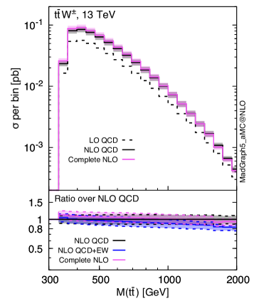
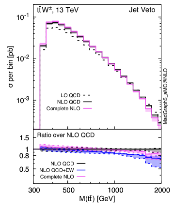
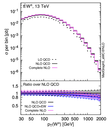
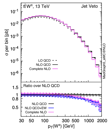
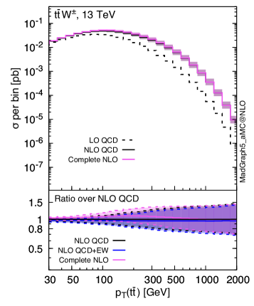
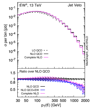
Figure 5: Differential distributions for $t\bar{t}W^{\pm}$ production at 13 TeV. For the plots on the right, the jet veto of eq. (12) has been applied. The main panels show the scale-uncertainty bands for ${\rm LO}_{\rm QCD}+{\rm NLO}_{\rm QCD}$ (black) and ${\rm LO}+{\rm NLO}$ (pink), and central value of ${\rm LO}_{\rm QCD}$; In the lower inset the scale-uncertainty bands are normalised to the ${\rm LO}_{\rm QCD}+{\rm NLO}_{\rm QCD}$ central value and also the ${\rm LO}_{\rm QCD}+{\rm NLO}_{\rm QCD}+{\rm NLO}_{\rm EW}$ prediction (blue) is displayed.

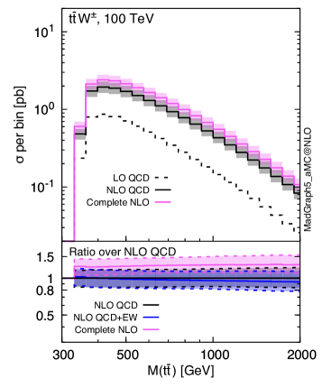
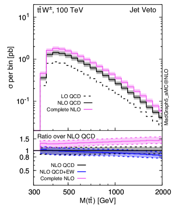
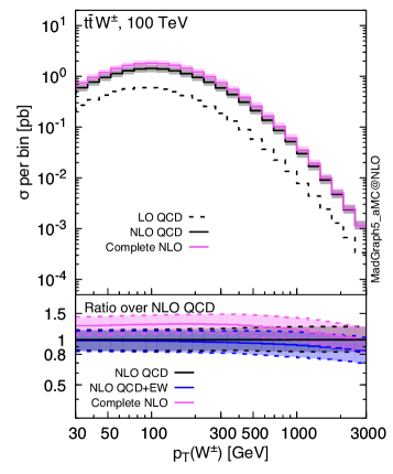
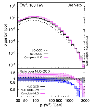
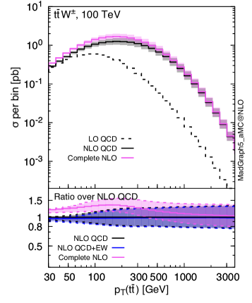
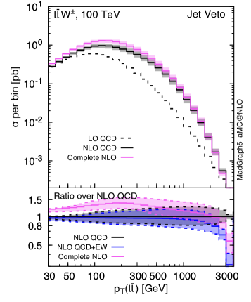
Figure 6: Same as Fig. 5 but for 100 TeV collisions.

Further details about individual ${\rm NLO}_{i}$ contributions at the differential level are given in Fig. 7 (13 TeV) and Fig. 8 (100 TeV). In the plots we show all the $\delta_{{\rm NLO}_{i}}(\mu)$ for $\mu=\mu_{c}\equiv H_{T}/2$ (solid line), $\mu=\mu_{c}/2$ (dashed line) and $\mu=2\mu_{c}$ (dotted line). We show the same distributions (with and without veto) as in Figs. 5 and 6. We remark again that the $\delta_{{\rm NLO}_{i}}(\mu)$ do not show directly scale uncertainties since the value of $\mu$ is varied both in the numerator and the denominator of $\delta$. On the other hand, we can directly see that also at the differential level the relative sizes of both ${\rm NLO}_{2}$ and ${\rm NLO}_{3}$ w.r.t. the ${\rm LO}_{\rm QCD}$ are almost insensitive to the value of the scale; the corresponding solid, dashed and dotted lines are almost indistinguishable. As expected, also at the differential level the impact of the ${\rm NLO}_{4}$ is completely negligible for the whole range of the distributions considered.

As could already have been concluded by comparing the dashed and solid black lines in Figs. 5 and 6, the NLO QCD corrections are not at all a constant over phase space. The solid black lines in Figs. 7 and 8 make this very clear. In particular for the $p_{T}(t\bar{t})$ distributions without the jet veto (lower left plots), the ${\rm NLO}_{1}\equiv{\rm NLO}_{\rm QCD}$ contribution easily becomes as large as the ${\rm LO}_{1}\equiv{\rm LO}_{\rm QCD}$ and increases to more than an order of magnitude larger than ${\rm LO}_{1}$ at large transverse momenta in 100 TeV collisions. But also for $p_{T}(W^{\pm})$ we see large NLO QCD corrections, in particular at 100 TeV. On the other hand, for $m(t\bar{t})$ the NLO QCD corrections are mostly flat, in particular at 13 TeV. With the jet veto (plots on the right) the situation changes quite dramatically. The NLO QCD corrections are, in general, under much better control, even though one can see that the extreme tails in the $p_{T}(W^{\pm})$ and $p_{T}(t\bar{t})$ at 100 TeV the ${\rm NLO}_{\rm QCD}$ contributions decrease rapidly and are starting to be strongly influenced by logarithms related to the jet-veto scale. If one would look at even larger transverse momenta, or, equivalently, reduce the jet-veto scale, these logarithms will grow and eventually fixed-order perturbation theory would break down, showing the need for resummation of these jet-veto logarithms.

Since these plots are normalised w.r.t. the ${\rm LO}_{1}$ (c.f., the lower insets of Figs. 5 and 6 which are normalised to ${\rm LO}_{1}+{\rm NLO}_{1}$), one can clearly see the effects of the NLO EW corrections, i.e., the ${\rm NLO}_{2}$, independently from the NLO QCD corrections. One sees the typical EW Sudakov logarithms: negligible effects at the percent level at small and moderate $t\bar{t}$ invariant masses and $W^{\pm}$ and $t\bar{t}$ transverse momenta, but growing rapidly with increasing values of the observables, to about $-$20% at $m(t\bar{t})\simeq 2000$ GeV and $-$40% at $p_{T}(W^{\pm})\simeq p_{T}(t\bar{t})\simeq 2000$ GeV. The fact that the NLO EW corrections are smaller for $m(t\bar{t})$ in comparison to $p_{T}(W^{\pm})$ and $p_{T}(t\bar{t})$ is no surprise since the impact of the EW Sudakov logarithms is related to the number of invariants that are large for the observable considered. Typically, for large invariant masses, there need to be fewer large invariants than for producing large transverse momenta. The size of the NLO EW corrections relative to the ${\rm LO}_{1}$ is quite similar for 13 TeV and 100 TeV collisions. Moreover, by comparing the distributions with and without the jet veto we also see that their sizes are hardly influenced by the jet veto.

At variance with the ${\rm NLO}_{2}$ term, at 13 TeV the ${\rm NLO}_{3}$ contribution is much more constant w.r.t. the ${\rm LO}_{1}$ over the whole phase space. Indeed, for the $m(t\bar{t})$ the $\delta_{{\rm NLO}_{3}}$ is effectively a constant, increasing the ${\rm LO}_{1}$ cross section by about 12% (which is reduced by applying the jet veto to about 9%). Similarly, for the $p_{T}(W^{\pm})$ distribution, the ${\rm NLO}_{3}$ correction is fairly flat. On the other hand, the $p_{T}(t\bar{t})$ does show some kinematic dependence in the $\delta_{{\rm NLO}_{3}}$ ratio. It is small at small transverse momenta, increases at intermediate values and, in particular when the jet veto is applied, it decreases again at large values of $p_{T}(t\bar{t})$. This is consistent with what we found in the comparing the ${\rm LO}_{\rm QCD}+{\rm NLO}_{\rm QCD}$ and NLO QCD + EW predictions in Fig. 5. At 100 TeV the ${\rm NLO}_{3}$ contributions are large and the $\delta_{{\rm NLO}_{3}}$ plots are not at all flat in the phase space. As at 13 TeV, the effects are most dramatic in the $p_{T}(t\bar{t})$ distributions, which show a large hump at around 500 GeV (1 TeV) with (without) the jet veto. However, as discussed before, without a jet veto, at large $p_{T}(t\bar{t})$ the ${\rm NLO}_{\rm QCD}$ corrections is giant and is even the dominant contribution among all the ${\rm(N)LO}_{i}$ ones, including the ${\rm LO}_{1}$. For this reason, although $\delta_{{\rm NLO}_{2}}$ and $\delta_{{\rm NLO}_{3}}$ are large at high $p_{T}(t\bar{t})$, results at ${\rm LO}_{\rm QCD}+{\rm NLO}_{\rm QCD}$, ${\rm LO}_{\rm QCD}+{\rm NLO}_{\rm QCD}+{\rm NLO}_{\rm EW}$, and ${\rm LO}+{\rm NLO}$ accuracies are very close to each other; the three predictions are all dominated by ${\rm NLO}_{\rm QCD}$, while $\delta_{{\rm NLO}_{i}}$ are normalised to ${\rm LO}_{\rm QCD}$.

The application of a jet veto as in eq. (12) may be exploited in BSM analyses such as the one described in ref. Dror:2015nkp ; rather than requiring a forward jet it may be possible to observe enhancements in the $tW^{\pm}\to tW^{\pm}$ scattering directly in $t\bar{t}W^{\pm}$ production by vetoing hard central jets.

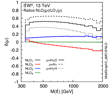
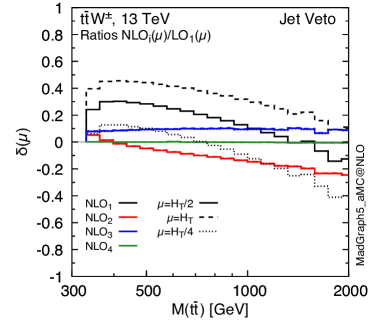
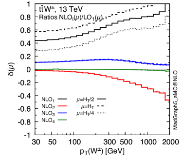
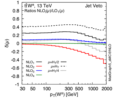
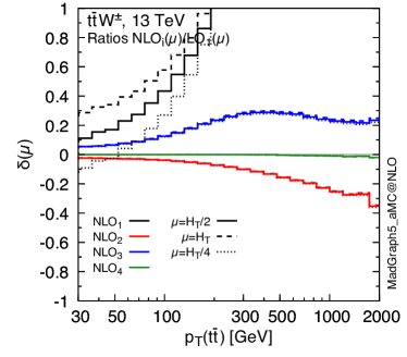
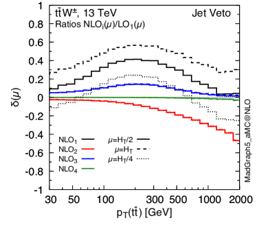
Figure 7: Individual ${\rm NLO}_{i}$ contributions to $t\bar{t}W^{\pm}$ production at 13 TeV normalised to ${\rm LO}_{1}\equiv{\rm LO}_{\rm QCD}$, for different values of the scale $\mu$ for the same distributions as considered in Fig. 5. These plots do not directly show scale uncertainties. Note that ${\rm NLO}_{1}\equiv{\rm NLO}_{\rm QCD}$ and ${\rm NLO}_{2}\equiv{\rm NLO}_{\rm EW}$.

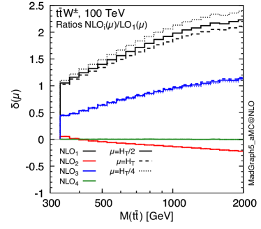
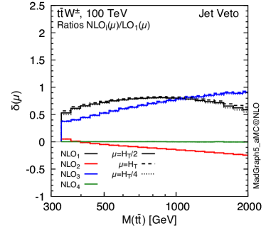
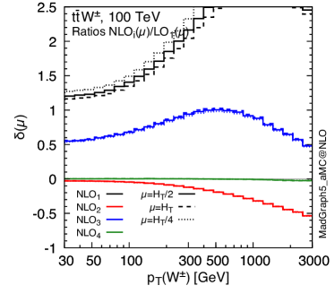
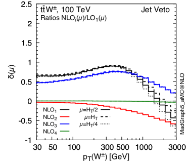
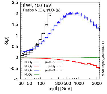
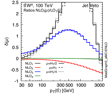
Figure 8: Same as Fig. 7 but for 100 TeV collisions.

3.3 Results for $pp\to t\bar{t}t\bar{t}$ production

$\sigma[\textrm{fb}]$	LO${}_{\textrm{QCD}}$	${\rm LO}_{\rm QCD}+{\rm NLO}_{\rm QCD}$	LO	${\rm LO}+{\rm NLO}$	$\frac{{\rm LO}(+{\rm NLO})}{{\rm LO}_{\rm QCD}(+{\rm NLO}_{\rm QCD})}$
$\mu=H_{T}/4$	$6.83{}^{+70\%}_{-38\%}$	$11.12{}^{+19\%}_{-23\%}$	$7.59{}^{+64\%}_{-36\%}$	$11.97{}^{+18\%}_{-21\%}$	$1.11\,(1.08)$

Table 5: Cross section for $pp\to t\bar{t}t\bar{t}$ at 13 TeV in various approximations.

$\sigma[\textrm{pb}]$	LO${}_{\textrm{QCD}}$	${\rm LO}_{\rm QCD}+{\rm NLO}_{\rm QCD}$	LO	${\rm LO}+{\rm NLO}$	$\frac{{\rm LO}(+{\rm NLO})}{{\rm LO}_{\rm QCD}(+{\rm NLO}_{\rm QCD})}$
$\mu=H_{T}/4$	$2.37{}^{+49\%}_{-31\%}$	$3.98{}^{+18\%}_{-19\%}$	$2.63{}^{+44\%}_{-28\%}$	$4.18{}^{+17\%}_{-17\%}$	$1.11\,(1.05)$

Table 6: Same as in Tab. 5 but for 100 TeV.

Similarly to the previous section, we start by presenting predictions for $t\bar{t}t\bar{t}$ total cross sections at 13 and 100 TeV proton–proton collisions and then we discuss results at the differential level. Using a layout that is similar to Tab. 1, in Tab. 5 we show 13 TeV predictions at ${\rm LO}_{\rm QCD}$, ${\rm LO}_{\rm QCD}+{\rm NLO}_{\rm QCD}$, ${\rm LO}$ and ${\rm LO}+{\rm NLO}$ accuracies. We also display the ${\rm LO}/{\rm LO}_{\rm QCD}$ and, in brackets, $({\rm LO}+{\rm NLO})/({\rm LO}_{\rm QCD}+{\rm NLO}_{\rm QCD})$ ratios. Results at 100 TeV are in Tab. 6. In Tab. 7, similarly to Tab. 3, we show 13 TeV predictions for the $\delta_{{\rm(N)LO}_{i}}(\mu)$ ratios, and analogous results at 100 TeV are in Tab. 8.

As can be seen in Tabs. 5 and 6, the scale dependence is very large at ${\rm LO}_{\rm QCD}$ and ${\rm LO}$ accuracy and it is strongly reduced both in the NLO QCD and complete-NLO predictions to about 20%. Nevertheless, it is still larger than the impact of the non-purely-QCD contributions, which is also reduced moving from LO to NLO accuracy, halved in the 100 TeV case. At the inclusive level, the difference between ${\rm LO}+{\rm NLO}$ and ${\rm LO}_{\rm QCD}+{\rm NLO}_{\rm QCD}$ predictions is well within their respective scale uncertainties, especially at 100 TeV where this difference is merely $5\%$ of the ${\rm LO}_{\rm QCD}+{\rm NLO}_{\rm QCD}$ result. However, the numbers in Tabs. 5 and 6 hide the most important feature of the complete-NLO result, i.e., very large and scale-dependent cancellations among the ${\rm(N)LO}_{i}$ terms with $i\geq 2$. This will become clear from the discussion in the next paragraph.

$\delta[\%]$	$\mu=H_{T}/8$	$\mu=H_{T}/4$	$\mu=H_{T}/2$
LO2	$-26.0$	$-28.3$	$-30.5$
LO3	$32.6$	$39.0$	$45.9$
LO4	$0.2$	$0.3$	$0.4$
LO5	$0.02$	$0.03$	$0.05$
NLO1	$14.0$	$62.7$	$103.5$
NLO2	$8.6$	$-3.3$	$-15.1$
NLO3	$-10.3$	$1.8$	$16.1$
NLO4	$2.3$	$2.8$	$3.6$
NLO5	$0.12$	$0.16$	$0.19$
NLO6	$<0.01$	$<0.01$	$<0.01$
${\rm NLO}_{2}+{\rm NLO}_{3}$	$-1.7$	$-1.6$	$0.9$

Table 7: $t\bar{t}t\bar{t}$: $\sigma_{{\rm(N)LO}_{i}}/\sigma_{{\rm LO}_{\rm QCD}}$ ratios at 13 TeV, for different values of $\mu=\mu_{r}=\mu_{f}$.

As anticipated in sec. 2, in $t\bar{t}t\bar{t}$ production the ${\rm LO}_{2}$ and ${\rm LO}_{3}$ contributions are not so suppressed w.r.t. the ${\rm LO}_{\rm QCD}$, at variance with $t\bar{t}W^{\pm}$ production (see Tabs. 7 and 8, c.f. Tabs. 3 and 4). For $t\bar{t}t\bar{t}$ production, due to sizeable contributions from the EW $tt\to tt$ scattering, ${\rm LO}_{2}$ and ${\rm LO}_{3}$ can induce corrections of the order $-30\%$ and $+40\%$ on top of the ${\rm LO}_{1}$, respectively. Therefore, also the ${\rm NLO}_{2}$ and ${\rm NLO}_{3}$ contributions are large, since they contain “QCD corrections” to ${\rm LO}_{2}$ and ${\rm LO}_{3}$ terms, respectively. The fact that a large fraction of ${\rm NLO}_{2}$ and ${\rm NLO}_{3}$ contributions is of QCD origin can be understood by the $\mu$-dependencies of $\delta_{{\rm NLO}_{2}}$ and $\delta_{{\rm NLO}_{3}}$ ratios, which, as can be seen in Tabs. 7 and 8, are very large. Indeed, ${\rm NLO}_{2}$ and ${\rm NLO}_{3}$ terms involve explicit logarithms of $\mu$ that compensate the PDF and $\alpha_{s}$ scale dependence at ${\rm LO}_{2}$ and ${\rm LO}_{3}$ accuracy, respectively. Thus, in $t\bar{t}t\bar{t}$ production, at variance with most of the other production processes studied in the literature, quoting the relative size of ${\rm NLO}_{\rm EW}\equiv{\rm NLO}_{2}$ or ${\rm NLO}_{3}$ corrections without specifying the QCD-renormalisation and factorisation scale is simply meaningless. Moreover, $\delta_{{\rm NLO}_{2}}$ and $\delta_{{\rm NLO}_{3}}$ corrections can separately be very large, easily reaching $\pm 15\%$ (depending on the value of $\mu$). Surprisingly, for our central value of the renormalisation and factorisation scales, the $\delta_{{\rm NLO}_{2}}$ and $\delta_{{\rm NLO}_{3}}$ are almost zero, particularly for 13 TeV. On the other hand, if we had taken $H_{T}/2$ or even $m_{t\bar{t}t\bar{t}}$ as our central scale choice, the ${\rm NLO}_{2}$ and ${\rm NLO}_{3}$ corrections relative to the ${\rm LO}_{1}$, $\delta_{{\rm NLO}_{2}}$ and $\delta_{{\rm NLO}_{3}}$, would have been much larger. Still, even for the central value $\mu=H_{T}/4$, the corrections are much larger than foreseen, especially for $\delta_{{\rm NLO}_{3}}$ which naively is expected to be of order $\alpha_{s}^{3}\alpha^{2}/\alpha_{s}^{4}=\alpha^{2}/\alpha_{s}\sim 0.1\%$ level. On the other hand, the relative cancellation observed between ${\rm NLO}_{2}$ and ${\rm NLO}_{3}$ contributions is even larger than in the case of ${\rm LO}_{2}$ and ${\rm LO}_{3}$. As can be seen in the last rows of Tabs. 7 and 8, at the inclusive level the sum of the ratios $\delta_{{\rm NLO}_{2}}+\delta_{{\rm NLO}_{3}}$ is not only small, but also stable under scale variation, resulting in corrections of at most a few percents w.r.t. the ${\rm LO}_{\rm QCD}$. Furthermore, particularly at 13 TeV, $\delta_{{\rm NLO}_{2}}+\delta_{{\rm NLO}_{3}}$ receives also additional cancellations when summed to $\delta_{{\rm NLO}_{4}}$, which itself is much larger than the expected $\alpha_{s}^{2}\alpha^{3}/\alpha_{s}^{4}=\alpha^{3}/\alpha_{s}^{2}\sim 0.01\%$ level. To the best of our understanding, these cancellations are accidental.

These large and accidental cancellations among the ${\rm(N)LO}_{i}$ terms with $i>1$ are particularly relevant from a BSM perspective, since the level of these cancellations may be altered by new physics. As an example, we can refer to the case of an anomalous $y_{t}$ coupling, which, as we have already mentioned, has been considered in the tree-level analysis of ref. Cao:2016wib . Terms proportional to $y_{t}^{2}$ are present in all the ${\rm(N)LO}_{i}$ with $i\geq 2$ and terms proportional to $y_{t}^{4}$ are present in all the ${\rm(N)LO}_{i}$ with $i\geq 3$, but also terms proportional to $y_{t}^{6}$ are present for any $i\geq 3$. Moreover, also contributions proportional to $y_{t}$, $y_{t}^{3}$ and $y_{t}^{5}$ are possible. Similar considerations apply also to other new physics effects in $t\bar{t}t\bar{t}$ production (see, e.g., ref. Zhang:2017mls and references therein for scenarios already analysed in the literature).

In order to understand the hierarchy of the different ${\rm(N)LO}_{i}$ contributions, it is important to note that at 13 TeV and especially at 100 TeV the total cross section is dominated by the $gg$ initial state (see, e.g., ref. Maltoni:2015ena ). For this reason, the ${\rm LO}_{4}$, ${\rm LO}_{5}$, ${\rm NLO}_{5}$ and ${\rm NLO}_{6}$ contributions, which are vanishing for the $gg$ initial state, are much smaller than the other contributions. The modest scale dependence of $\delta_{{\rm NLO}_{4}}$ is also induced by this feature; the ${\rm NLO}_{4}$ contribution mainly arises from “EW corrections” to $gg$-induced ${\rm LO}_{3}$ contributions, which do not have any explicit dependence on $\mu$; and therefore the scale dependence of the ${\rm NLO}_{4}$ follows the scale dependence of the ${\rm LO}_{3}$ to a large extent.

$\delta[\%]$	$\mu=H_{T}/8$	$\mu=H_{T}/4$	$\mu=H_{T}/2$
LO2	$-18.7$	$-20.7$	$-22.8$
LO3	$26.3$	$31.8$	$37.8$
LO4	$0.05$	$0.07$	$0.09$
LO5	$0.03$	$0.05$	$0.08$
NLO1	$33.9$	$68.2$	$98.0$
NLO2	$-0.3$	$-5.7$	$-11.6$
NLO3	$-3.9$	$1.7$	$8.9$
NLO4	$0.7$	$0.9$	$1.2$
NLO5	$0.12$	$0.14$	$0.16$
NLO6	$<0.01$	$<0.01$	$<0.01$
${\rm NLO}_{2}+{\rm NLO}_{3}$	$-4.2$	$-4.0$	$2.7$

Table 8: $t\bar{t}t\bar{t}$: $\sigma_{{\rm(N)LO}_{i}}/\sigma_{{\rm LO}_{\rm QCD}}$ ratios at 100 TeV, for different values of $\mu=\mu_{r}=\mu_{f}$.

Differential distributions

We now move to the description of the results at the differential level, where we consider the following distributions: the invariant mass of the four (anti)top quarks $m(t\bar{t}t\bar{t})$ (Fig. 9), the sum of the transverse masses of all the particles in the final state $H_{T}$ as defined in eq. (11) (Fig. 10), the transverse momenta of the hardest of the two top quarks $p_{T}(t_{1})$ (Fig. 11), and the rapidity of the softest one $y(t_{2})$ (Fig. 12). At variance with the case of $t\bar{t}W^{\pm}$ production in sec. 3.2, we organise plots according to the observable considered. In the figures we display 13 TeV results on the left and 100 TeV results on the right. In the upper plots of each of these figures we provide predictions at different levels of accuracy, using a similar layout as in Figs. 5 and 6, which is described in detail in sec. 3.2. Also for $t\bar{t}t\bar{t}$ production, comparisons among the scale uncertainties of the ${\rm LO}_{\rm QCD}$ and ${\rm LO}_{\rm QCD}+{\rm NLO}_{\rm QCD}$ result have been documented in detail in ref. Maltoni:2015ena for 13 TeV, so they are not repeated here. Individual contributions from the different ${\rm(N)LO}_{i}$ terms are instead displayed in the central and lower plots. In the central plots we show the $\delta_{{\rm(N)LO}_{i}}(\mu)$, see eq. (13), with $\mu=\mu_{c}\equiv H_{T}/4$, while the lower plots focus on ${\rm NLO}_{2}$ and ${\rm NLO}_{3}$ contributions and their sum featuring large cancellations. In particular, we show $\delta_{{\rm NLO}_{2}}(\mu)$, $\delta_{{\rm NLO}_{3}}(\mu)$ and their sum for $\mu=\mu_{c}$ (solid line), $\mu=\mu_{c}/2$ (dashed line) and $\mu=2\mu_{c}$ (dotted line). In practice, the dark-blue and red solid lines are the same quantities in the middle and lower plots. Once again, we remark that the $\delta_{{\rm NLO}_{i}}(\mu)$ ratio does not show directly the scale uncertainty since the value of $\mu$ is varied both in the numerator and the denominator of $\delta$.

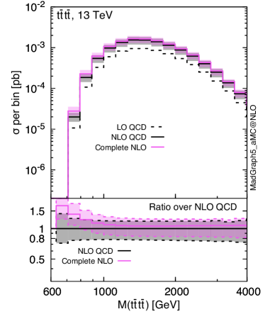
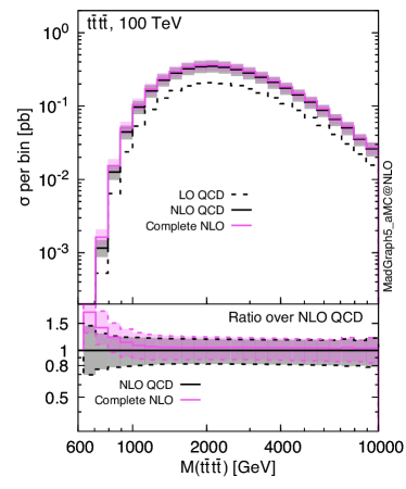
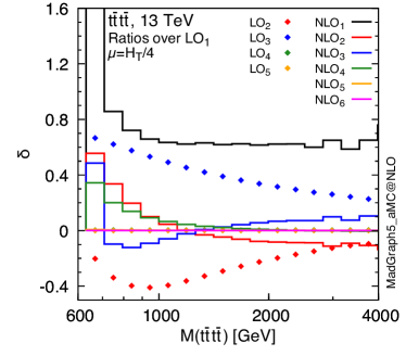
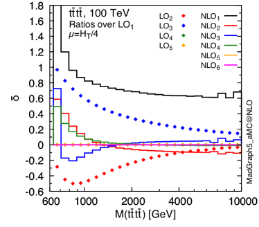
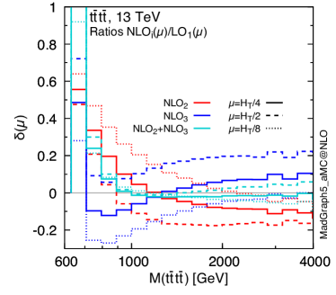
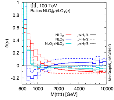
Figure 9: The $m(t\bar{t}t\bar{t})$ distribution in $t\bar{t}t\bar{t}$ production. Left: 13 TeV. Right: 100 TeV. Upper plots: scale uncertainty bands (same layout as the plots in Figs. 5 and 6). Central plots: individual ${\rm(N)LO}_{i}$ contributions normalised to ${\rm LO}_{1}\equiv{\rm LO}_{\rm QCD}$. Lower plots: same as central plots but only with ${\rm NLO}_{2}$, ${\rm NLO}_{3}$, and their sum, at different values of the scale $\mu$. These lower plots do not show scale uncertainties. Note that ${\rm NLO}_{1}\equiv{\rm NLO}_{\rm QCD}$ and ${\rm NLO}_{2}\equiv{\rm NLO}_{\rm EW}$.

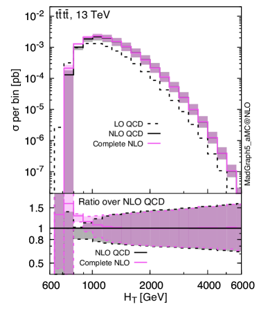
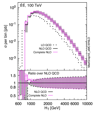
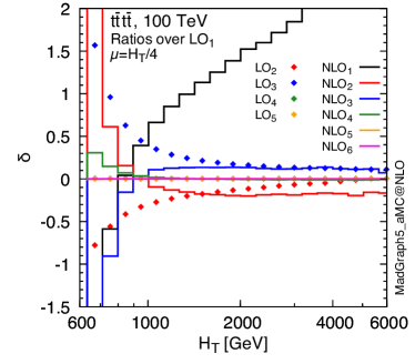
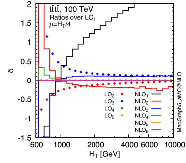
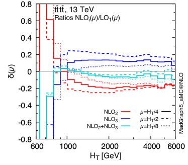
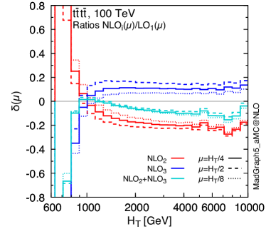
Figure 10: The $H_{T}$ distribution in $t\bar{t}t\bar{t}$ production. See the caption of Fig. 9 for the description of the plots.

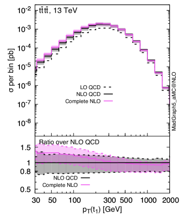
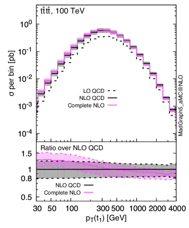
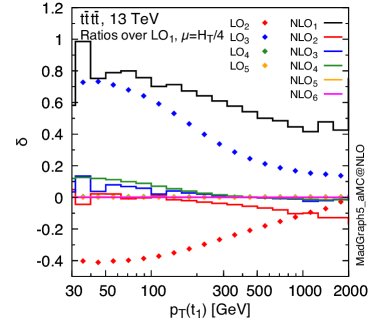
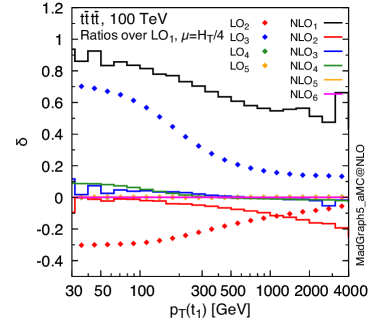
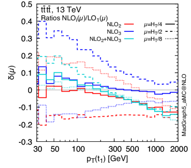
Figure 11: The $p_{T}(t_{1})$ distribution in $t\bar{t}t\bar{t}$ production. See the caption of Fig. 9 for the description of the plots.

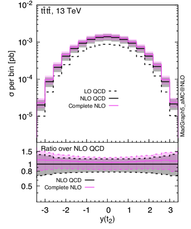
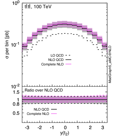
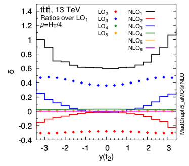
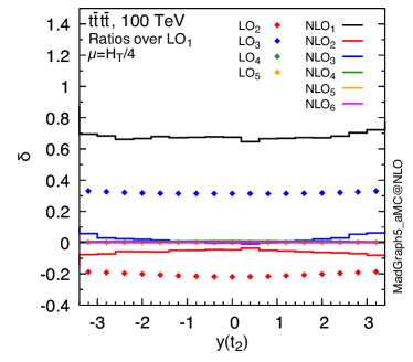
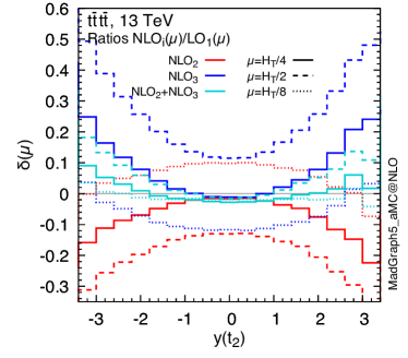
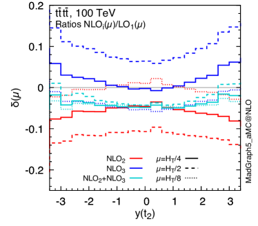
Figure 12: The $y(t_{2})$ distribution in $t\bar{t}t\bar{t}$ production. See the caption of Fig. 9 for the description of the plots.

Away from the threshold region, i.e., $m(t\bar{t}t\bar{t})>$ 900 GeV, the complete-NLO prediction for the four-top invariant-mass distribution is very close to the NLO QCD one, with an almost constant increase of about 10%, both at 13 and 100 TeV, see upper plots in Fig. 9. This increase is well within the uncertainty bands of either of the predictions. On the other hand, in the threshold region the enhancement of the cross section due to terms with ${\rm(N)LO}_{i}$, with $i>1$, is much larger than for the inclusive results. In this region the central value of the complete-NLO predictions lies outside the ${\rm LO}_{1}+{\rm NLO}_{1}$ uncertainty band. From the central plots of Fig. 9, it can be seen that the ${\rm(N)LO}_{2}$ and ${\rm(N)LO}_{3}$ contributions are individually sizeable w.r.t. ${\rm LO}_{\rm QCD}$ and their relative impact has a large dependence on kinematics, easily reaching several tens of percents in certain regions of phase space.

As anticipated from the inclusive results, there are large cancellations in the distributions among ${\rm LO}_{2}$ and ${\rm LO}_{3}$ contributions and especially among ${\rm NLO}_{2}$, ${\rm NLO}_{3}$ ones; the latter are explicitly shown in the lower plots. In particular, although the corresponding $\delta_{{\rm(N)LO}_{i}}$ terms individually depend on the value of $m(t\bar{t}t\bar{t})$, they lead for $m(t\bar{t}t\bar{t})>$ 900 GeV to the aforementioned constant increase of about 10% of the complete-NLO prediction w.r.t. the NLO QCD result. As can be seen in the central plots, the $\delta_{{\rm LO}_{2}}$ is negative, it is about $-10\%$ at $m(t\bar{t}t\bar{t})\simeq$ 4000 GeV and further decreases for smaller invariant masses, reaching about $-40\%$ at $m(t\bar{t}t\bar{t})\simeq$ 900 GeV. On the other hand, the $\delta_{{\rm LO}_{3}}$ is positive, and very close to the absolute value of $\delta_{{\rm LO}_{2}}$ plus a constant 12 (at 13 TeV) or 16 (at 100 TeV) percentage points. Moreover, even though also the $\delta_{{\rm NLO}_{2}}$ and $\delta_{{\rm NLO}_{3}}$ are depending quite strongly on the value of $m(t\bar{t}t\bar{t})$, they sum to almost a constant $-1\%$ (at 13 TeV) and $-4\%$ (at 100 TeV). Therefore, indeed, the entire sum ${\rm LO}_{2}+{\rm LO}_{3}+{\rm NLO}_{2}+{\rm NLO}_{3}$ is almost a constant 10% correction to the ${\rm LO}_{1}+{\rm NLO}_{1}$ —away from the threshold region.

In the threshold region, the situation is quite different. While the $\delta_{{\rm LO}_{3}}$ keeps increasing closer and closer to threshold, the derivative of $\delta_{{\rm LO}_{2}}$ reverses sign at $m(t\bar{t}t\bar{t})\simeq$ 900 GeV. In other words, the $\delta_{{\rm LO}_{2}}$ also starts to increase closer and closer to threshold. The same is true for the corrections induced by ${\rm NLO}_{2}$ and ${\rm NLO}_{3}$ contributions: the $\delta_{{\rm NLO}_{3}}$ sharply increases close to threshold. Hence, the delicate cancellation among the ${\rm LO}_{2}$ and ${\rm LO}_{3}$ (and ${\rm NLO}_{2}$ and ${\rm NLO}_{3}$) contributions completely breaks down in this region of phase space. Moreover, also the ${\rm NLO}_{4}$ reaches several tens of percent close to threshold and should not be neglected when studying this region of phase space. Conversely, also at the differential level, ${\rm LO}_{4}$, ${\rm LO}_{5}$, ${\rm NLO}_{5}$ and ${\rm NLO}_{6}$ contributions are negligible.

There are two different physical effects at the origin of the large NLO corrections in the threshold region. First, also the ${\rm LO}_{2}$ and ${\rm LO}_{3}$ contributions are larger in this region and thus their “QCD corrections”, which respectively enter the ${\rm NLO}_{2}$ and ${\rm NLO}_{3}$ contributions, preserve this increment w.r.t. the rest of the phase space. Second, the exchange of $Z$ or Higgs bosons among top quarks, or in general among heavy particles, can lead to Sommerfeld enhancements when the top quarks are in a non-relativistic regime. This effect has already been documented in refs. Kuhn:2013zoa ; Beneke:2015lwa for the case of top-quark pair production and in refs. Degrassi:2016wml ; Bizon:2016wgr ; Maltoni:2017ims for the exchange of a virtual Higgs boson between an on-shell Higgs boson and another on-shell heavy particle. The threshold region forces each $t\bar{t}$, $tt$ or $\bar{t}\bar{t}$ pair to potentially lead to this kind of effect. These large “EW corrections” on top of ${\rm LO}_{1}$ and ${\rm LO}_{2}$ terms lead to additional sizeable contributions to ${\rm NLO}_{2}$ and ${\rm NLO}_{3}$, respectively. Moreover, since also ${\rm LO}_{3}$ is large, via this kind of “EW corrections” even ${\rm NLO}_{4}$ is very large and incredibly enhanced w.r.t. the result at the inclusive level.

The lower plots in Fig. 9 further confirm the QCD origin of the ${\rm NLO}_{2}$ and ${\rm NLO}_{3}$ contributions. In order to explain this, we remind the reader that the scale dependence of the ${\rm LO}_{2}$ and ${\rm LO}_{3}$ contributions is the typical one, i.e., ${\rm LO}_{2}$ and ${\rm LO}_{3}$ absolute values become smaller when the scales are increased. In the plots we see that for ${\rm NLO}_{3}$ the (dark blue) dashed lines are larger than the solid lines, which are in turn larger than dotted lines, while in the case of ${\rm NLO}_{2}$ the order is the reversed. Since the ${\rm LO}_{2}$ is negative, the ${\rm NLO}_{2}$ term reduces the $\mu$ dependence of the ${\rm LO}_{2}$ one and, similarly, the ${\rm NLO}_{3}$ term reduces the $\mu$ dependence of the ${\rm LO}_{3}$ one. Moreover, these plots confirm that also at the differential level there are large cancellations among the ${\rm NLO}_{2}$ and ${\rm NLO}_{3}$ terms and that the $\delta_{{\rm NLO}_{2}}+\delta_{{\rm NLO}_{3}}$ sum has a much smaller scale dependence than the two separate addends. In other words, the remarkable cancellations among the ${\rm NLO}_{2}$ and ${\rm NLO}_{3}$ corrections are not only present for the central value of $\mu$, as already concluded from the middle plots in the discussion above, but also for their scale dependencies. Notably, these cancellations are present over a very large region of phase space. Also, if we had chosen, e.g., $H_{T}/2$ as our central scale (dashed lines in the lower plot), the ${\rm NLO}_{2}$ and ${\rm NLO}_{3}$ curves in the middle plots would have been much further apart, leading to much larger cancellations, since their sum would hardly have changed at all.

Compared to the invariant-mass distribution of the four tops, the case of the $H_{T}$ distribution (Fig. 10) is similar in many respects. In particular, from the upper plots, we see that again only in the threshold region there is a sizeable difference between the NLO QCD predictions and the complete-NLO ones. It should be noted, though, that above the peak in the distribution, $H_{T}\gtrsim$ 1500 GeV, the difference between the two predictions is very small, their central values as well as the scale uncertainties are lying almost exactly on top of each other. Just as in the case of the $m(t\bar{t}t\bar{t})$, the middle plots show that this is rather due to large and accidental cancellations among the various ${\rm(N)LO}_{i}$ with $i>1$ contributions, which can individually reach several tens of percent.

Close to the $H_{T}\simeq 4m_{t}$ threshold, the ${\rm NLO}_{i}$ contributions are in general reverted in sign w.r.t. the ${\rm LO}_{i}$ ones and receive particularly large enhancements in absolute value. This feature is due to large negative QCD Sudakov logarithms that appear in the limit $H_{T}\to 4m_{t}$. Indeed, since $H_{T}$ includes in its definition the momentum of the possible extra jet, it effectively acts as a tight jet veto in this limit. Thus, “QCD corrections” involves large and negative contributions that have to be resummed. The effect is so large that in the first bin of the central plots of Fig. 10, the ${\rm LO}_{\rm QCD}+{\rm NLO}_{\rm QCD}$ prediction is negative and should not be trusted. This is a well-known instability of fixed-order perturbative calculations. Similar but smaller effects originate also from “EW corrections”, due to the effective veto on the real emission.

It is also interesting to note how the $\mu$-dependence of $\delta_{{\rm NLO}_{2}}$ reduces for large values of $H_{T}$ (see bottom plots of Fig. 10). We can see in the central plots that $\delta_{{\rm LO}_{2}}$ is very small in this phase-space region, which means that the dominant ${\rm NLO}_{2}$ contribution cannot be originated by “QCD corrections” on top of ${\rm LO}_{2}$. Rather, it is mainly induced by “EW corrections” on top of the ${\rm LO}_{\rm QCD}$ term. Thus, we recover the typical situation, which we found also in $t\bar{t}W^{\pm}$ production, where $\delta_{{\rm NLO}_{2}}\equiv\delta_{{\rm NLO}_{\rm EW}}$ is almost independent of the value of $\mu$.

An example of an observable in which the cancellation between the ${\rm NLO}_{2}$ and ${\rm NLO}_{3}$ is less complete in the whole range considered is the transverse momentum of the hardest of the two top quarks, shown in Fig. 11. Similarly to $m(t\bar{t}t\bar{t})$ and $H_{T}$, close to the threshold region, $p_{T}(t_{1})\lesssim$ 300 GeV, the complete-NLO predictions are above the NLO QCD ones, reaching $\sim\!\!25\%$ at very small transverse momenta. On the other hand, for $p_{T}(t_{1})\gtrsim$ 300 GeV, the complete-NLO corrections on top of the NLO QCD are growing negative and become about $-10\%$ in the tails of the distributions shown. From the middle plots, which refer to the case $\mu=H_{T}/4$, it becomes clear which orders are responsible for this behaviour. At small transverse momenta there are large positive corrections from the ${\rm LO}_{3}$ (up to about 70% on top of ${\rm LO}_{1}$) and to a lesser extent the ${\rm NLO}_{4}$, which is itself slightly larger than ${\rm NLO}_{3}$. ${\rm LO}_{2}$ is also large, but negative, about $-40\%$ on top of ${\rm LO}_{1}$, only partially cancelling the large positive contribution from ${\rm LO}_{3}$. Accidentally, ${\rm NLO}_{2}$ corrections are instead almost equal to zero. Adding together all these contributions and taking also into account that the ${\rm NLO}_{1}$ yields a positive 80% correction, we indeed find close to the threshold a correction of about 25% from complete-NLO result on top of the NLO QCD one. On the other hand, with increasing $p_{T}$, all the corrections quickly reduce (in absolute value), although not all in a uniform way. The exception is the $\delta_{{\rm NLO}_{2}}$, which steadily grows negative. Thus, at transverse momenta in the TeV range, the ${\rm NLO}_{2}\equiv{\rm NLO}_{\rm EW}$ becomes the dominant correction to the NLO QCD predictions. At first sight, this seems to be the standard situation with NLO EW corrections completely dominated by Sudakov logarithms, which we also observed in the ${\rm NLO}_{2}$ curves for the $pp\to t\bar{t}W^{\pm}$ process, see Figs. 7 and 8. However, looking at the lower plots, it is clear that this cannot be the complete story. If the ${\rm NLO}_{2}$ had been completely dominated by “EW corrections” on top of the ${\rm LO}_{1}$, the $\delta_{{\rm NLO}_{2}}$ ratio would have been (almost) scale independent. Conversely, although the scale dependence of $\delta_{{\rm NLO}_{2}}$ does decrease with increasing transverse momenta, it remains anyway sizeable even in the far tail of the distribution. Therefore, a non-negligible part of ${\rm NLO}_{2}$ is due to “QCD corrections” on top of the ${\rm LO}_{2}$ also in the far tail. For these reasons, although in this phase-space region the individual and summed $\delta_{{\rm NLO}_{i}}$ with $i>1$ are not at all constant, the scale dependence of $\delta_{{\rm NLO}_{2}}+\delta_{{\rm NLO}_{3}}$ remains very small. The non-constant part seems to be the “EW corrections” entering the ${\rm NLO}_{2}$, which are dominated by large and negative Sudakov logarithms and do not introduce a new scale dependence w.r.t. the ${\rm LO}_{1}$.

From the $y(t_{2})$ distribution (Fig. 12) we can see that, besides the threshold region, a non-negligible difference between NLO QCD and complete-NLO predictions is present also at 13 TeV (not 100 TeV) in the peripheral region of the softest of the top quark quarks. The $y(t_{2})$ distribution is also the only one, among those considered, where the impact of the different ${\rm(N)LO}_{i}$ terms is qualitatively different at 13 and 100 TeV. While the ${\rm LO}_{i}$ corrections are rather flat at both 13 and 100 TeV, ${\rm NLO}_{i}$ corrections are flat only at 100 TeV; the ${\rm NLO}_{i}$ corrections for 13 TeV yield large effects in the peripheral region. The origin of this difference is the range of Bjorken-$x$ probed in the PDFs, which is indeed very different at 13 and 100 TeV. While at 13 TeV the peripheral region is typically associated with tops that have large rapidities also in the $t\bar{t}t\bar{t}$ rest frame, at 100 TeV it is more likely that they originate from partonic initial states that are boosted w.r.t. the proton–proton reference frame. For this reason the $y(t_{2})$ distribution is flatter at 100 TeV than at 13 TeV, where large rapidities are strongly suppressed in a Born-like kinematics and therefore they are also much more sensitive to effects due to real emission from ${\rm NLO}_{i}$ contributions. However, as before, the ${\rm NLO}_{2}$ and ${\rm NLO}_{3}$ contributions almost cancel, resulting in at most $\sim\!\!10\%$ effects w.r.t. the ${\rm LO}_{1}$ in the far forward and backward regions.

Given our findings, we suggest that the study of the $\mu$-dependence of $\delta_{{\rm NLO}_{i}}$ can be a very useful procedure for identifying the nature of ${\rm NLO}_{i}$ corrections in numerical calculations. For higher values of $i$, the $\Sigma_{{\rm NLO}_{i}}(\mu)/\Sigma_{{\rm LO}_{i-1}}(\mu)$ may be even more appropriate given the different numerical sizes of the ${\rm LO}_{i}$ terms and of their dependence on the running of $\alpha_{s}$. For instance, we verified that in $t\bar{t}t\bar{t}$ production both $\Sigma_{{\rm NLO}_{4}}/\Sigma_{{\rm LO}_{3}}$ and $\Sigma_{{\rm NLO}_{6}}/\Sigma_{{\rm LO}_{5}}$ are very mildly scale-dependent at inclusive and differential level. Indeed, both can be considered almost purely “EW corrections”; the latter by construction and the former due to the dominance of the $gg$ initial-state. Conversely, we do not find this feature in the $\Sigma_{{\rm NLO}_{5}}/\Sigma_{{\rm LO}_{4}}$ ratio, since ${\rm LO}_{4}$ and ${\rm LO}_{5}$ contributions are both small but comparable in size and thus $\Sigma_{{\rm NLO}_{5}}$ receives large “QCD corrections” on top of ${\rm LO}_{5}$ contributions.

In summary, at the inclusive and the differential levels complete-NLO results for $t\bar{t}t\bar{t}$ production are well within the NLO QCD uncertainties. For the observables presented here, there are no large qualitative differences between results at 13 and 100 TeV, except in the peripheral regions of the rapidity of the second hardest top quark. However, for all observables very large cancellations among the different perturbative orders are present both at the inclusive and differential level. Their individual sizes w.r.t. the ${\rm LO}_{\rm QCD}$ prediction are also strongly dependent on the scale definition. All these arguments point to the fact that in any BSM analysis involving $t\bar{t}t\bar{t}$ production contributions from all NLO corrections can be relevant. Thus, they should be taken into account, at least in the estimate of the theory uncertainty.

4 Conclusions

In this paper we have presented the complete-NLO predictions for $t\bar{t}W^{\pm}$ and $t\bar{t}t\bar{t}$ production at 13 and 100 TeV in proton–proton collisions. All the seven $\mathcal{O}(\alpha_{s}^{i}\alpha^{j})$ contributions with $i+j=3,4$ and $j\geq 1$ for $t\bar{t}W^{\pm}$ production and all the eleven $\mathcal{O}(\alpha_{s}^{i}\alpha^{j})$ contributions with $i+j=4,5$ have been calculated exactly without any approximation. We have shown that complete-NLO corrections involve large contributions beyond the NLO EW accuracy for both the $t\bar{t}W^{\pm}$ and $t\bar{t}t\bar{t}$ production processes

In $t\bar{t}W^{\pm}$ production we find that the $\mathcal{O}(\alpha_{s}\alpha^{3})$ contributions, denoted as ${\rm NLO}_{3}$ in this article, are larger than NLO EW corrections and have opposite sign. They are of the order 12(70)% of the LO at 13(100) TeV, with a strong dependence on particular kinematic variables such as $p_{T}(W^{\pm})$ and $p_{T}(t\bar{t})$, but not $m(t\bar{t})$. Thus, they are several orders of magnitude larger than the values naively expected from their coupling orders, i.e., ${\rm NLO}_{3}/{\rm LO}\gg\alpha^{2}/\alpha_{s}\sim 0.1\%$. The main reason is the opening of the $tW\to tW$ scattering in the ${\rm NLO}_{3}$. Since the NLO QCD corrections are dominated by hard radiation, applying a jet veto suppresses the ${\rm NLO}_{\rm QCD}$ contributions considerably. Conversely, the ${\rm NLO}_{3}$ (and the NLO EW corrections) are affected to a much lesser extent, resulting in large corrections on top of the NLO-QCD result. At 13 TeV, applying a 100 GeV central jet veto, the central value of the complete-NLO prediction is typically outside the NLO QCD scale-uncertainty band. At 100 TeV, the uncertainty bands of these two predictions do not even touch. Besides their relevance for the SM and reliable comparisons with current and future measurements, these results further support the proposal of the BSM analysis described in ref. Dror:2015nkp , showing a possible sensitivity to higher-dimensional operators in $tW\to tW$ scattering directly in $t\bar{t}W^{\pm}$ production. Rather than requiring a jet and considering $tW\to tW$ scattering as a Born process, our results suggest that the sensitivity may be increased by directly considering $t\bar{t}W^{\pm}$ production and vetoing additional jets.

In $t\bar{t}t\bar{t}$ production, LO contributions of $\mathcal{O}(\alpha_{s}^{3}\alpha)$ are about $-$25-30% of the purely-QCD $\mathcal{O}(\alpha_{s}^{4})$ ones, while $\mathcal{O}(\alpha_{s}^{2}\alpha^{2})$ contributions are about $+$30-45%, depending on the scale choice. For this reason, we find that the $\mathcal{O}(\alpha_{s}^{4}\alpha)$ (the NLO EW corrections, or ${\rm NLO}_{2}$) as well as the $\mathcal{O}(\alpha_{s}^{3}\alpha^{2})$ (denoted as ${\rm NLO}_{3}$ in this article) contributions are also large. Moreover, since they receive large contributions from “QCD corrections” (and thus $\alpha_{s}$ and PDF renormalisation) on top of respectively $\mathcal{O}(\alpha_{s}^{3}\alpha)$ and $\mathcal{O}(\alpha_{s}^{2}\alpha^{2})$ terms, they strongly depend on the scale definition. At 13 TeV, their relative impact w.r.t. purely-QCD $\mathcal{O}(\alpha_{s}^{4})$ contribution varies in both cases between $\pm 15\%$. On the other hand, their sum reduces to a rather small $\pm$1-2%, and is almost independent from the QCD scale choice and kinematics. Qualitatively similar results are found also at 100 TeV. The size of the cancellations is quite remarkable, unexpected, and, to the best of our knowledge, accidental. Thus, a calculation of only part of the complete-NLO results would be missing important contributions. These large cancellations between the corrections and the reduced scale dependencies of their sum are not present very close to threshold. In this region of phase space, complete-NLO results are sizeably different from those at NLO QCD accuracy and even contributions of $\mathcal{O}(\alpha_{s}^{2}\alpha^{3})$ (denoted as ${\rm NLO}_{4}$ in this article) are found to be of the order of several tens of percents of the LO. Besides their relevance for the SM and reliable comparisons with current and future measurements, our calculations show that the possible impact of NLO corrections should be critically considered for studies such as ref. Cao:2016wib , where $t\bar{t}t\bar{t}$ production has been proposed as candidate, in conjunction with $t\bar{t}H$ production, for an independent determination of the Yukawa coupling of the top quark and the Higgs-boson total decay width. Similar considerations apply to other BSM studies involving $t\bar{t}t\bar{t}$ production: the various contributions from NLO corrections are large and the cancellations among them could be spoiled by BSM effects. This should be taken into account at least in the estimate of the theory uncertainties.

In this work we have also shown that the study of the $\mu$-dependence of the quantity $\delta_{{\rm NLO}_{i}}\equiv\Sigma_{{\rm NLO}_{i}}(\mu)/\Sigma_{{\rm LO}_{1}}(\mu)$ can be a very useful procedure for identifying the nature of ${\rm NLO}_{i}$ corrections in numerical calculations. A large scale dependence is a signal of “QCD corrections” on top of the ${\rm LO}_{i}$ contribution, while a scale independence for $\delta_{{\rm NLO}_{i}}$ points to “EW corrections” on top of the ${\rm LO}_{i-1}$ contributions. For higher values of $i$, the $\Sigma_{{\rm NLO}_{i}}(\mu)/\Sigma_{{\rm LO}_{i-1}}(\mu)$ may be even more appropriate given the possible different numerical sizes of the ${\rm LO}_{i}$ terms and of their dependence on the running of $\alpha_{s}$.

As a final remark, we want to remind the reader that the three known cases where NLO corrections from supposedly subleading EW contributions are large, $pp\to t\bar{t}W^{\pm}$, $pp\to t\bar{t}t\bar{t}$ and $pp\to W^{+}W^{+}jj$ with leptonic $W^{+}$ decays Biedermann:2017bss , involve very different mechanisms. In $t\bar{t}W^{\pm}$ production it is the opening of $tW\to tW$ scattering via the real emission in the ${\rm NLO}_{3}$. In $t\bar{t}t\bar{t}$ production it is mainly the “QCD corrections” on top of EW $tt\to tt$ scattering, which gives large contributions already at the LO. In $W^{+}W^{+}jj$ production it is instead the large EW Sudakov logarithmic corrections featured by the formally most subleading NLO contribution Biedermann:2016yds together with the relatively large size (especially when standard VBS cuts are applied) of the purely EW $W^{+}W^{+}$ scattering component.

References

- (1) J. M. Campbell and R. K. Ellis, An Update on vector boson pair production at hadron colliders, Phys. Rev. D60 (1999) 113006, [hep-ph/9905386].
- (2) G. Cullen, N. Greiner, G. Heinrich, G. Luisoni, P. Mastrolia, G. Ossola, T. Reiter, and F. Tramontano, Automated One-Loop Calculations with GoSam, Eur. Phys. J. C72 (2012) 1889, [arXiv:1111.2034].
- (3) G. Cullen et al., GS-2.0: a tool for automated one-loop calculations within the Standard Model and beyond, Eur. Phys. J. C74 (2014), no. 8 3001, [arXiv:1404.7096].
- (4) S. Badger, B. Biedermann, P. Uwer, and V. Yundin, Numerical evaluation of virtual corrections to multi-jet production in massless QCD, Comput. Phys. Commun. 184 (2013) 1981–1998, [arXiv:1209.0100].
- (5) F. Cascioli, P. Maierhofer, and S. Pozzorini, Scattering Amplitudes with Open Loops, Phys. Rev. Lett. 108 (2012) 111601, [arXiv:1111.5206].
- (6) S. Actis, A. Denner, L. Hofer, A. Scharf, and S. Uccirati, Recursive generation of one-loop amplitudes in the Standard Model, JHEP 04 (2013) 037, [arXiv:1211.6316].
- (7) S. Actis, A. Denner, L. Hofer, J.-N. Lang, A. Scharf, and S. Uccirati, RECOLA: REcursive Computation of One-Loop Amplitudes, Comput. Phys. Commun. 214 (2017) 140–173, [arXiv:1605.01090].
- (8) T. Gleisberg, S. Hoeche, F. Krauss, M. Schonherr, S. Schumann, F. Siegert, and J. Winter, Event generation with SHERPA 1.1, JHEP 02 (2009) 007, [arXiv:0811.4622].
- (9) G. Bevilacqua, M. Czakon, M. V. Garzelli, A. van Hameren, A. Kardos, C. G. Papadopoulos, R. Pittau, and M. Worek, HELAC-NLO, Comput. Phys. Commun. 184 (2013) 986–997, [arXiv:1110.1499].
- (10) V. Hirschi, R. Frederix, S. Frixione, M. V. Garzelli, F. Maltoni, and R. Pittau, Automation of one-loop QCD corrections, JHEP 05 (2011) 044, [arXiv:1103.0621].
- (11) J. Alwall, R. Frederix, S. Frixione, V. Hirschi, F. Maltoni, O. Mattelaer, H. S. Shao, T. Stelzer, P. Torrielli, and M. Zaro, The automated computation of tree-level and next-to-leading order differential cross sections, and their matching to parton shower simulations, JHEP 07 (2014) 079, [arXiv:1405.0301].
- (12) S. Alioli, P. Nason, C. Oleari, and E. Re, A general framework for implementing NLO calculations in shower Monte Carlo programs: the POWHEG BOX, JHEP 06 (2010) 043, [arXiv:1002.2581].
- (13) S. Platzer and S. Gieseke, Dipole Showers and Automated NLO Matching in Herwig++, Eur. Phys. J. C72 (2012) 2187, [arXiv:1109.6256].
- (14) S. Kallweit, J. M. Lindert, P. Maierh fer, S. Pozzorini, and M. Sch nherr, NLO electroweak automation and precise predictions for W+multijet production at the LHC, JHEP 04 (2015) 012, [arXiv:1412.5157].
- (15) S. Kallweit, J. M. Lindert, P. Maierhofer, S. Pozzorini, and M. Sch nherr, NLO QCD+EW predictions for V + jets including off-shell vector-boson decays and multijet merging, JHEP 04 (2016) 021, [arXiv:1511.08692].
- (16) B. Biedermann, S. Br uer, A. Denner, M. Pellen, S. Schumann, and J. M. Thompson, Automation of NLO QCD and EW corrections with Sherpa and Recola, Eur. Phys. J. C77 (2017) 492, [arXiv:1704.05783].
- (17) S. Frixione, V. Hirschi, D. Pagani, H. S. Shao, and M. Zaro, Weak corrections to Higgs hadroproduction in association with a top-quark pair, JHEP 09 (2014) 065, [arXiv:1407.0823].
- (18) S. Frixione, V. Hirschi, D. Pagani, H. S. Shao, and M. Zaro, Electroweak and QCD corrections to top-pair hadroproduction in association with heavy bosons, JHEP 06 (2015) 184, [arXiv:1504.03446].
- (19) R. Frederix, S. Frixione, V. Hirschi, D. Pagani, H.-S. Shao, and M. Zaro, The complete NLO corrections to dijet hadroproduction, JHEP 04 (2017) 076, [arXiv:1612.06548].
- (20) M. Chiesa, N. Greiner, and F. Tramontano, Automation of electroweak corrections for LHC processes, J. Phys. G43 (2016), no. 1 013002, [arXiv:1507.08579].
- (21) N. Greiner and M. Schoenherr, NLO QCD+EW corrections to diphoton production in association with a vector boson, arXiv:1710.11514.
- (22) G. Heinrich, QCD calculations for the LHC: status and prospects, 2017, arXiv:1710.04998.
- (23) C. Anastasiou, C. Duhr, F. Dulat, F. Herzog, and B. Mistlberger, Higgs Boson Gluon-Fusion Production in QCD at Three Loops, Phys. Rev. Lett. 114 (2015) 212001, [arXiv:1503.06056].
- (24) F. A. Dreyer and A. Karlberg, Vector-Boson Fusion Higgs Production at Three Loops in QCD, Phys. Rev. Lett. 117 (2016) no.7, 072001 [arXiv:1606.00840].
- (25) M. Czakon, D. Heymes, A. Mitov, D. Pagani, I. Tsinikos, and M. Zaro, Top-pair production at the LHC through NNLO QCD and NLO EW, JHEP 10, 186 (2017), [arXiv:1705.04105].
- (26) B. Biedermann, A. Denner, and M. Pellen, Complete NLO corrections to scattering and its irreducible background at the LHC, arXiv:1708.00268.
- (27) B. Biedermann, A. Denner and M. Pellen, Large electroweak corrections to vector-boson scattering at the Large Hadron Collider, Phys. Rev. Lett. 118 (2017) 261801, [arXiv:1611.02951].
- (28) CMS Collaboration, Measurement of top pair-production in association with a W or Z boson in pp collisions at 13 TeV, Tech. Rep. CMS-PAS-TOP-17-005, CERN, Geneva, 2017.
- (29) ATLAS Collaboration, M. Aaboud et al., Measurement of the and production cross sections in multilepton final states using 3.2 fb-1 of collisions at = 13 TeV with the ATLAS detector, Eur. Phys. J. C77 (2017), no. 1 40, [arXiv:1609.01599].
- (30) CMS Collaboration, Search for the standard model production of four top quarks with same-sign and multilepton final states in proton-proton collisions at , Tech. Rep. CMS-PAS-TOP-17-009, CERN, Geneva, 2017.
- (31) J. R. Andersen et al., Les Houches 2015: Physics at TeV Colliders Standard Model Working Group Report, in 9th Les Houches Workshop on Physics at TeV Colliders (PhysTeV 2015) Les Houches, France, June 1-19, 2015, 2016. arXiv:1605.04692.
- (32) R. Frederix, S. Frixione, V. Hirschi, D. Pagani, H.-S. Shao, and M. Zaro, in preparation.
- (33) J. A. Dror, M. Farina, E. Salvioni, and J. Serra, Strong tW Scattering at the LHC, JHEP 01 (2016) 071, [arXiv:1511.03674].
- (34) Q.-H. Cao, S.-L. Chen, and Y. Liu, Probing Higgs Width and Top Quark Yukawa Coupling from and Productions, Phys. Rev. D95 (2017), no. 5 053004, [arXiv:1602.01934].
- (35) M. V. Garzelli, A. Kardos, C. G. Papadopoulos, and Z. Trocsanyi, t and t Z Hadroproduction at NLO accuracy in QCD with Parton Shower and Hadronization effects, JHEP 11 (2012) 056, [arXiv:1208.2665].
- (36) J. M. Campbell and R. K. Ellis, production and decay at NLO, JHEP 07 (2012) 052, [arXiv:1204.5678].
- (37) F. Maltoni, M. L. Mangano, I. Tsinikos, and M. Zaro, Top-quark charge asymmetry and polarization in production at the LHC, Phys. Lett. B736 (2014) 252–260, [arXiv:1406.3262].
- (38) F. Maltoni, D. Pagani, and I. Tsinikos, Associated production of a top-quark pair with vector bosons at NLO in QCD: impact on searches at the LHC, JHEP 02 (2016) 113, [arXiv:1507.05640].
- (39) H. T. Li, C. S. Li, and S. A. Li, Renormalization group improved predictions for production at hadron colliders, Phys. Rev. D90 (2014), no. 9 094009, [arXiv:1409.1460].
- (40) A. Broggio, A. Ferroglia, G. Ossola, and B. D. Pecjak, Associated production of a top pair and a W boson at next-to-next-to-leading logarithmic accuracy, JHEP 09 (2016) 089, [arXiv:1607.05303].
- (41) A. Kulesza, L. Motyka, D. Schwartl nder, T. Stebel, and V. Theeuwes, Soft gluon resummation for the associated production of a top quark pair with a W boson at the LHC, 2017, arXiv:1710.06810.
- (42) LHC Higgs Cross Section Working Group Collaboration, D. de Florian et al., Handbook of LHC Higgs Cross Sections: 4. Deciphering the Nature of the Higgs Sector, arXiv:1610.07922.
- (43) G. Bevilacqua and M. Worek, Constraining BSM Physics at the LHC: Four top final states with NLO accuracy in perturbative QCD, JHEP 07 (2012) 111, [arXiv:1206.3064].
- (44) S. Frixione, Z. Kunszt, and A. Signer, Three jet cross-sections to next-to-leading order, Nucl. Phys. B467 (1996) 399–442, [hep-ph/9512328].
- (45) S. Frixione, A General approach to jet cross-sections in QCD, Nucl. Phys. B507 (1997) 295–314, [hep-ph/9706545].
- (46) R. Frederix, S. Frixione, F. Maltoni, and T. Stelzer, Automation of next-to-leading order computations in QCD: The FKS subtraction, JHEP 10 (2009) 003, [arXiv:0908.4272].
- (47) R. Frederix, S. Frixione, A. S. Papanastasiou, S. Prestel, and P. Torrielli, Off-shell single-top production at NLO matched to parton showers, JHEP 06 (2016) 027, [arXiv:1603.01178].
- (48) G. Ossola, C. G. Papadopoulos, and R. Pittau, Reducing full one-loop amplitudes to scalar integrals at the integrand level, Nucl. Phys. B763 (2007) 147–169, [hep-ph/0609007].
- (49) P. Mastrolia, E. Mirabella, and T. Peraro, Integrand reduction of one-loop scattering amplitudes through Laurent series expansion, JHEP 06 (2012) 095, [arXiv:1203.0291]. [Erratum: JHEP11,128(2012)].
- (50) G. Passarino and M. J. G. Veltman, One Loop Corrections for e+ e- Annihilation Into mu+ mu- in the Weinberg Model, Nucl. Phys. B160 (1979) 151–207.
- (51) A. I. Davydychev, A Simple formula for reducing Feynman diagrams to scalar integrals, Phys. Lett. B263 (1991) 107–111.
- (52) A. Denner and S. Dittmaier, Reduction schemes for one-loop tensor integrals, Nucl. Phys. B734 (2006) 62–115, [hep-ph/0509141].
- (53) G. Ossola, C. G. Papadopoulos, and R. Pittau, CutTools: A Program implementing the OPP reduction method to compute one-loop amplitudes, JHEP 03 (2008) 042, [arXiv:0711.3596].
- (54) T. Peraro, Ninja: Automated Integrand Reduction via Laurent Expansion for One-Loop Amplitudes, Comput. Phys. Commun. 185 (2014) 2771–2797, [arXiv:1403.1229].
- (55) V. Hirschi and T. Peraro, Tensor integrand reduction via Laurent expansion, JHEP 06 (2016) 060, [arXiv:1604.01363].
- (56) A. Denner, S. Dittmaier, and L. Hofer, Collier: a fortran-based Complex One-Loop LIbrary in Extended Regularizations, Comput. Phys. Commun. 212 (2017) 220–238, [arXiv:1604.06792].
- (57) A. Manohar, P. Nason, G. P. Salam, and G. Zanderighi, How bright is the proton? A precise determination of the photon parton distribution function, Phys. Rev. Lett. 117 (2016), no. 24 242002, [arXiv:1607.04266].
- (58) A. V. Manohar, P. Nason, G. P. Salam, and G. Zanderighi, The Photon Content of the Proton, arXiv:1708.01256.
- (59) J. Butterworth et al., PDF4LHC recommendations for LHC Run II, J. Phys. G43 (2016) 023001, [arXiv:1510.03865].
- (60) NNPDF Collaboration, R. D. Ball et al., Parton distributions for the LHC Run II, JHEP 04 (2015) 040, [arXiv:1410.8849].
- (61) L. A. Harland-Lang, A. D. Martin, P. Motylinski, and R. S. Thorne, Parton distributions in the LHC era: MMHT 2014 PDFs, Eur. Phys. J. C75 (2015), no. 5 204, [arXiv:1412.3989].
- (62) S. Dulat, T.-J. Hou, J. Gao, M. Guzzi, J. Huston, P. Nadolsky, J. Pumplin, C. Schmidt, D. Stump, and C. P. Yuan, New parton distribution functions from a global analysis of quantum chromodynamics, Phys. Rev. D93 (2016), no. 3 033006, [arXiv:1506.07443].
- (63) M. L. Mangano et al., Physics at a 100 TeV pp collider: Standard Model processes, CERN Yellow Report (2017), no. 3 1–254, [arXiv:1607.01831].
- (64) C. Zhang, Constraining operators from four-top production: a case for enhanced EFT sensitivity, arXiv:1708.05928.
- (65) J. H. K hn, A. Scharf, and P. Uwer, Weak Interactions in Top-Quark Pair Production at Hadron Colliders: An Update, Phys. Rev. D91 (2015), no. 1 014020, [arXiv:1305.5773].
- (66) M. Beneke, A. Maier, J. Piclum, and T. Rauh, Higgs effects in top anti-top production near threshold in annihilation, Nucl. Phys. B899 (2015) 180–193, [arXiv:1506.06865].
- (67) G. Degrassi, P. P. Giardino, F. Maltoni, and D. Pagani, Probing the Higgs self coupling via single Higgs production at the LHC, JHEP 12 (2016) 080, [arXiv:1607.04251].
- (68) W. Bizon, M. Gorbahn, U. Haisch, and G. Zanderighi, Constraints on the trilinear Higgs coupling from vector boson fusion and associated Higgs production at the LHC, JHEP 07 (2017) 083, [arXiv:1610.05771].
- (69) F. Maltoni, D. Pagani, A. Shivaji, and X. Zhao, Trilinear Higgs coupling determination via single-Higgs differential measurements at the LHC, arXiv:1709.08649.