IP/BBSR/2017-13

SISSA 53/2017/FISI

IPMU17-0154

IPPP/17/75

Addressing Neutrino Mixing Models with DUNE and T2HK

Sanjib Kumar Agarwalla${}^{\,a,b,c,}$, Sabya Sachi Chatterjee${}^{\,a,b,}$,

S. T. Petcov${}^{\,d,e,}$ and A. V. Titov${}^{\,d,f,}$

^a Institute of Physics, Sachivalaya Marg, Sainik School Post, Bhubaneswar 751005, India

^b Homi Bhabha National Institute, Training School Complex,
Anushakti Nagar, Mumbai 400085, India

^c International Centre for Theoretical Physics, Strada Costiera 11, 34151 Trieste, Italy

^d SISSA/INFN, Via Bonomea 265, 34136 Trieste, Italy

^e Kavli IPMU (WPI), University of Tokyo, 5-1-5 Kashiwanoha, 277-8583 Kashiwa, Japan

^f Institute for Particle Physics Phenomenology, Department of Physics, Durham University,
South Road, Durham DH1 3LE, United Kingdom

We consider schemes of neutrino mixing arising within the discrete symmetry approach to the well-known flavour problem. We concentrate on $3\nu$ mixing schemes in which the cosine of the Dirac CP violation phase $\delta_{\mathrm{CP}}$ satisfies a sum rule by which it is expressed in terms of three neutrino mixing angles $\theta_{12}$, $\theta_{23}$, and $\theta_{13}$, and a fixed real angle $\theta^{\nu}_{12}$, whose value depends on the employed discrete symmetry and its breaking. We consider five underlying symmetry forms of the neutrino mixing matrix: bimaximal (BM), tri-bimaximal (TBM), golden ratio A (GRA) and B (GRB), and hexagonal (HG). For each symmetry form, the sum rule yields specific prediction for $\cos\delta_{\mathrm{CP}}$ for fixed $\theta_{12}$, $\theta_{23}$, and $\theta_{13}$. In the context of the proposed DUNE and T2HK facilities, we study (i) the compatibility of these predictions with present neutrino oscillation data, and (ii) the potential of these experiments to discriminate between various symmetry forms.

1 Introduction and Motivation

All compelling neutrino oscillation data are compatible with $3\nu$ mixing [1], i.e., with existence of three light neutrino states $\nu_{1,2,3}$ with definite masses $m_{1,2,3}$, three orthogonal linear combinations of which form the three flavour neutrino states $\nu_{e}$, $\nu_{\mu}$ and $\nu_{\tau}$. The flavour neutrino (flavour antineutrino) oscillation probabilities in the case of $3\nu$ mixing are characterised, as is well known, by six fundamental parameters. In the standard parametrisation of the Pontecorvo, Maki, Nakagawa, Sakata (PMNS) neutrino mixing matrix [1], these are the solar, reactor, and atmospheric mixing angles, $\theta_{12}$, $\theta_{13}$, and $\theta_{23}$, respectively, the Dirac CP violation (CPV) phase, $\delta_{\mathrm{CP}}$, and the two independent mass squared differences, $\Delta m_{21}^{2}\equiv m_{2}^{2}-m_{1}^{2}$ and $\Delta m_{31}^{2}\equiv m_{3}^{2}-m_{1}^{2}$. The mixing angles $\theta_{12}$ and $\theta_{13}$ as well as the solar and the absolute value of the atmospheric neutrino mass squared differences, $\Delta m_{21}^{2}$ and $|\Delta m_{31}^{2}|$, respectively, have been measured in neutrino oscillation experiments with a relatively high precision [2, 3, 4]. The precision on $\theta_{23}$ is somewhat worse, the relative $1\sigma$ uncertainty on $\sin^{2}\theta_{23}$ being approximately 10%. At the same time, the octant of $\theta_{23}$ and the value of $\delta_{\mathrm{CP}}$ remain unknown. The sign of $\Delta m_{31}^{2}$, which is also undetermined, allows, as is well known, for two possible types of the neutrino mass spectrum: (i) with normal ordering (NO) if $\Delta m_{31}^{2}>0$, and (ii) with inverted ordering (IO) if $\Delta m_{31}^{2}<0$. In Table 1, we summarise the best fit values and $1\sigma$, $2\sigma$, $3\sigma$ ranges of the oscillation parameters obtained in one of the latest global analysis of the neutrino oscillation data [3]. In the case of IO spectrum, instead of $\Delta m_{31}^{2}$, we use the largest positive mass squared difference $\Delta m_{23}^{2}\equiv m_{2}^{2}-m_{3}^{2}$, which corresponds to $\Delta m_{31}^{2}$ of the NO spectrum. In particular, we see from Table 1 that for the NO mass spectrum, the values of $\delta_{\mathrm{CP}}\in(31\degree,137\degree)$ are already disfavoured at more than $3\sigma$ C.L., while the values of $\delta_{\mathrm{CP}}$ between $180\degree$ and $342\degree$ are allowed at $2\sigma$.

[b]Parameter Best fit $1\sigma$ range $2\sigma$ range $3\sigma$ range $\dfrac{\sin^{2}\theta_{12}}{10^{-1}}$ 2.97 2.81–3.14 2.65–3.34 2.50–3.54 $\dfrac{\sin^{2}\theta_{13}}{10^{-2}}$ (NO) 2.15 2.08–2.22 1.99–2.31 1.90–2.40 $\dfrac{\sin^{2}\theta_{13}}{10^{-2}}$ (IO) 2.16 2.07–2.24 1.98–2.33 1.90–2.42 $\dfrac{\sin^{2}\theta_{23}}{10^{-1}}$ (NO) 4.25 4.10–4.46 3.95–4.70 3.81–6.15 $\dfrac{\sin^{2}\theta_{23}}{10^{-1}}$ (IO) 5.89 4.17–4.48 $\oplus$ 5.67–6.05 3.99–4.83 $\oplus$ 5.33–6.21 3.84–6.36 $\delta_{\mathrm{CP}}$ [°] (NO) $248$ 212–290 180–342 0–31 $\oplus$ 137–360 $\delta_{\mathrm{CP}}$ [°] (IO) $236$ 202–292 166–338 0–27 $\oplus$ 124–360 $\dfrac{\Delta m_{21}^{2}}{10^{-5}~{}\mathrm{eV}^{2}}$ 7.37 7.21–7.54 7.07–7.73 6.93–7.96 $\dfrac{\Delta m_{31}^{2}}{10^{-3}~{}\mathrm{eV}^{2}}$ (NO) 2.56 2.53–2.60 2.49–2.64 2.45–2.69 [b]$\dfrac{\Delta m_{23}^{2}}{10^{-3}~{}\mathrm{eV}^{2}}$ (IO) 2.54 2.51–2.58 2.47–2.62 2.42–2.66

Table 1: The best fit values and $1\sigma$, $2\sigma$, 3$\sigma$ ranges of the neutrino oscillation parameters obtained in the global analysis of the neutrino oscillation data performed in [3]. NO (IO) stands for normal (inverted) ordering of the neutrino mass spectrum.

Understanding the origin of the patterns of neutrino oscillation parameters revealed by the data is one of the most challenging problems in neutrino physics. It is a part of the more general fundamental problem in particle physics of understanding the origins of flavour, i.e., the patterns of quark, charged lepton, and neutrino masses, and quark and lepton mixing. There exists a possibility that the high-precision measurements of the oscillation parameters may shed light on the origin of the observed pattern of neutrino mixing and lepton flavour. This would be the case if the observed form of neutrino (and possibly quark) mixing were determined by an underlying discrete flavour symmetry. One of the most striking features of the discrete symmetry approach to neutrino mixing and lepton flavour (see, e.g., [5, 6, 7] for reviews), is that it leads to (i) fixed predictions of the values of some of the neutrino mixing angles and the Dirac CPV phase $\delta_{\mathrm{CP}}$, and/or (ii) existence of correlations between some of the mixing angles and/or between the mixing angles and $\delta_{\mathrm{CP}}$ (see, e.g., [8, 9, 10, 11, 12, 13, 14, 15, 16, 17, 18, 19]). These correlations are often referred to as neutrino mixing sum rules. Most importantly, these sum rules can be tested using oscillation data [8, 9, 10, 11, 19, 15, 30, 29, 31].

Within the discrete flavour symmetry approach, the PMNS matrix is predicted to have an underlying symmetry form, where $\theta_{12}$, $\theta_{23}$, and $\theta_{13}$ have values which differ by sub-leading perturbative corrections from their respective measured values. The approach seems very natural in view of the fact that $U_{\rm PMNS}=U_{e}^{\dagger}\,U_{\nu}$, where $U_{e}$ and $U_{\nu}$ are $3\times 3$ unitary matrices which diagonalise the charged lepton and neutrino mass matrices. Typically (but not universally) the matrix $U_{\nu}$ has a certain symmetry form, while the matrix $U_{e}$ provides the corrections necessary to bring the symmetry values of the angles in $U_{\nu}$ to their experimentally measured values. A sum rule which relates $\cos\delta_{\mathrm{CP}}$ with $\theta_{12}$, $\theta_{23}$, and $\theta_{13}$, arising in this approach, depends on the underlying symmetry form of the PMNS matrix and on the form of the “correcting” matrix $U_{e}$.

In the present work, we will concentrate on a particular sum rule for $\cos\delta_{\mathrm{CP}}$ derived in [8], which holds for a rather broad class of discrete flavour symmetry models. According to this sum rule, $\cos\delta_{\mathrm{CP}}$ is expressed in terms of the three measured neutrino mixing angles and one fixed parameter $\theta^{\nu}_{12}$ determined by the underlying discrete symmetry. This sum rule has the following form:

$$\cos\delta_{\mathrm{CP}}=\frac{\tan\theta_{23}}{\sin 2\theta_{12}\,\sin\theta_{13}}\left[\cos 2\theta^{\nu}_{12}+\left(\sin^{2}\theta_{12}-\cos^{2}\theta^{\nu}_{12}\right)\left(1-\cot^{2}\theta_{23}\,\sin^{2}\theta_{13}\right)\right]\,.$$ (1.1)

In this study, we consider five widely discussed underlying symmetry forms of the neutrino mixing matrix, namely, bimaximal (BM) [32, 33, 34, 35], tri-bimaximal (TBM) [36, 37, 38, 39] (see also [40]), golden ratio type A (GRA) [41, 42, 43], golden ratio type B (GRB) [44, 45], and hexagonal (HG) [46, 47]. Each of these symmetry forms is characterised by a specific value of the angle $\theta^{\nu}_{12}$ entering into the sum rule given in eq. (1.1). Namely, $\theta^{\nu}_{12}=45\degree$ (or $\sin^{2}\theta^{\nu}_{12}=0.5$) for BM; $\theta^{\nu}_{12}=\arcsin(1/\sqrt{3})\approx 35\degree$ (or $\sin^{2}\theta^{\nu}_{12}=1/3$) for TBM; $\theta^{\nu}_{12}=\arctan(1/\phi)\approx 32\degree$ (or $\sin^{2}\theta^{\nu}_{12}\approx 0.276$) for GRA, $\phi=(1+\sqrt{5})/2$ being the golden ratio; $\theta^{\nu}_{12}=\arccos(\phi/2)=36\degree$ (or $\sin^{2}\theta^{\nu}_{12}\approx 0.345$) for GRB; and $\theta^{\nu}_{12}=30\degree$ (or $\sin^{2}\theta^{\nu}_{12}=0.25$) for HG.

First, in eq. (1.1), we use the best fit values of the neutrino mixing angles assuming NO case from Table 1 to calculate the best fit value of $\cos\delta_{\mathrm{CP}}$ for a given symmetry form which has a fixed value of $\theta^{\nu}_{12}$. We present the obtained values in Table 2.

Symmetry form	$\theta^{\nu}_{12}$ [°]	$\cos\delta_{\mathrm{CP}}$	$\delta_{\mathrm{CP}}$ [°]
[t]BM	$45$	unphysical	unphysical
TBM	$\arcsin(1/\sqrt{3})\approx 35$	$-0.16$	$\phantom{1}99\lor 261$
GRA	$\arctan(1/\phi)\approx 32$	$\phantom{-}0.21$	$\phantom{1}78\lor 282$
GRB	$\arccos(\phi/2)=36$	$-0.24$	$104\lor 256$
HG	$30$	$\phantom{-}0.39$	$\phantom{1}67\lor 293$

Table 2: The best fit values of $\cos\delta_{\mathrm{CP}}$ and $\delta_{\mathrm{CP}}$ from the sum rule in eq. (1.1) for the different symmetry forms. The mixing angles $\theta_{12}$, $\theta_{23}$, and $\theta_{13}$ have been fixed to their NO best fit values from Table 1. The $\phi$ stands for the golden ratio: $\phi=(1+\sqrt{5})/2$. See text for further details.

For each symmetry form, the predicted value of $\cos\delta_{\mathrm{CP}}$ gives rise to two values of $\delta_{\mathrm{CP}}$ located symmetrically with respect to zero, which are also given in Table 2. Further, we calculate errors on these values by varying $\theta_{12}$, $\theta_{23}$, and $\theta_{13}$ (one at a time) in their $3\sigma$ experimentally allowed ranges for NO as given in Table 1 and fixing the two remaining angles to their best fit values. We summarise the obtained intervals of values of $\delta_{\mathrm{CP}}$ in Table 3.

Symmetry form	Intervals for $\delta_{\mathrm{CP}}$ [°] obtained varying
	$\theta_{12}$ in $3\sigma$	$\theta_{23}$ in $3\sigma$	$\theta_{13}$ in $3\sigma$
[t]BM	150–180 $\lor$ 180–210	unphysical	unphysical
TBM	179–119 $\lor$ 241–281	198–107 $\lor$ 253–262	98–101 $\lor$ 259–2621
GRA	1157–95 $\lor$ 265–303	1176–78 $\lor$ 282–284	77.6–77.9 $\lor$ 282.1–282.4
GRB	184–125 $\lor$ 235–276	102–114 $\lor$ 246–258	103–106 $\lor$ 254–25711
HG	1145–84 $\lor$ 276–315	1160–68 $\lor$ 292–300	1166–68 $\lor$ 292–29411

Table 3: The intervals for $\delta_{\mathrm{CP}}$ due to the present $3\sigma$ uncertainties in the values of the neutrino mixing angles. The quoted intervals are obtained varying one mixing angle in its corresponding $3\sigma$ range for the NO spectrum and fixing the other two angles to their NO best fit values.

In the case of the BM symmetry form, the obtained best fit value of $\cos\delta_{\mathrm{CP}}=-1.26$ is unphysical. This reflects the fact that the BM symmetry form does not provide a good description of the present best fit values of the neutrino mixing angles, as discussed in [13]. As can be seen from Table 3, current uncertainties on the mixing angles allow us to accommodate physical values of $\cos\delta_{\mathrm{CP}}$ for the BM symmetry form. For instance, fixing $\sin^{2}\theta_{13}$ and $\sin^{2}\theta_{23}$ to their best fit values, $\cos\delta_{\mathrm{CP}}=-1$ requires $\sin^{2}\theta_{12}=0.3343$, which is the upper bound of the corresponding $2\sigma$ allowed range of $\sin^{2}\theta_{12}$ (see Table 1).

A rather detailed analysis of the predictions for $\cos\delta_{\mathrm{CP}}$ of the sum rule in eq. (1.1) has been performed in Refs. [9, 10]. In particular, likelihood profiles for $\cos\delta_{\mathrm{CP}}$ for each symmetry form have been presented using the current and prospective precision on the neutrino mixing parameters (see Figs. 12 and 13 in [9]). In the present work, using the potential of the future long-baseline (LBL) neutrino oscillation experiments, namely, Deep Underground Neutrino Experiment (DUNE) and Tokai to Hyper-Kamiokande (T2HK), we study in detail (i) to what degree the sum rule predictions for $\cos\delta_{\mathrm{CP}}$ are compatible with the present neutrino oscillation data, and (ii) how well the considered symmetry forms, BM, TBM, GRA, GRB, and HG, can be discriminated from each other.

The layout of the article is as follows. In Section 2, we take a first glance at the sum rule predictions. In Section 3, we give a short description of the planned DUNE and T2HK experiments and provide expected event rates for both the set-ups. Section 4 contains details of the statistical analysis. In Section 5, we present and discuss results of this analysis. More specifically, in subsection 5.1, we test the compatibility between the considered symmetry forms and present oscillation data. Next, in subsection 5.2, we explore the potential of DUNE, T2HK, and their combination to distinguish between the symmetry forms in question under the assumption that one of them is realised in Nature. In subsection 5.3, we consider the BM symmetry form using the values of the mixing angles for which this form is viable, and study at which C.L. it can be distinguished from the other symmetry forms considered. We conclude in Section 6. Appendix A discusses the issue of external priors on $\sin^{2}\theta_{12}$ and $\sin^{2}\theta_{13}$. In Appendix B, we show the impact of marginalisation over $\Delta m_{31}^{2}$. Finally, in Appendix C, we study the compatibility of the considered symmetry forms with any potentially true values of $\sin^{2}\theta_{23}$ and $\delta_{\mathrm{CP}}$ in the context of DUNE and T2HK.

2 A First Glance at the Sum Rule Predictions

Let us first take a closer look at the sum rule predictions for $\delta_{\mathrm{CP}}$ summarised in Tables 2 and 3. Several important points that can be made from these two tables and the current global data (see Table 1) are in order.

• The parameter $\theta^{\nu}_{12}$ has a fixed value for each symmetry form as given in Table 2. For fixed choices of $\theta_{12}$, $\theta_{23}$, $\theta_{13}$, and $\theta^{\nu}_{12}$, eq. (1.1) predicts a certain value of $\cos\delta_{\mathrm{CP}}$, which gives rise to two values of $\delta_{\mathrm{CP}}$ (see fourth column of Table 2).

• The complementarity [52] between the modern reactor (Daya Bay, RENO, and Double Chooz) and accelerator (T2K and NO$\nu$A) data has enabled us to probe the parameter space for $\delta_{\mathrm{CP}}$. Already, the latest global data have disfavoured values of $\delta_{\mathrm{CP}}\in(31\degree,137\degree)$ at $3\sigma$ C.L. for NO (see Table 1). From Table 3, we see that out of the three mixing angles, the $3\sigma$ allowed range of $\theta_{12}$ causes the largest uncertainty in $\delta_{\mathrm{CP}}$ predicted by eq. (1.1). But, note that, all the symmetry forms except BM predict one of the ranges of $\delta_{\mathrm{CP}}$ in the interval of $31\degree$ to $137\degree$, which has been already ruled out at $3\sigma$. Therefore, we will not consider these ranges further in our study, and we will only consider the values of $\delta_{\mathrm{CP}}$ in the interval of $180\degree$ to $360\degree$.

• Further, we notice from Tables 1 and 3 that for TBM and GRB, the predicted intervals of $\delta_{\mathrm{CP}}$ lie within the $1\sigma$ experimentally allowed range. For BM, GRA, and HG, the intervals of interest fall within the $2\sigma$ range. Now, it would be quite interesting to assess the sensitivity of the future LBL experiments in discriminating various symmetry forms, which is the main thrust of the present work.

• T2HK and DUNE will not be able to constrain $\theta_{12}$, which causes the largest uncertainty in predicting the range of $\delta_{\mathrm{CP}}$ (see Table 3). However, the proposed JUNO experiment will provide a high-precision measurement of $\sin^{2}\theta_{12}$ with a relative $1\sigma$ uncertainty of 0.7%. Therefore, we impose a prior on $\sin^{2}\theta_{12}$ expected from JUNO, which we will discuss later in detail in Section 4 and in Appendix A.

• Table 3 shows that the sum rule predictions depend to some extent on $\theta_{23}$. Therefore, we vary this angle both in data and in fit. The LBL experiments themselves are sensitive to $\theta_{23}$. Thus, we do not impose any external prior on this angle (see details in Section 4).

• The experiments under discussion are sensitive to $\theta_{13}$ through the appearance channels ${\nu_{\mu}}\to{\nu_{e}}$ and ${\bar{\nu}_{\mu}}\to{\bar{\nu}_{e}}$. Therefore, the role of an external prior on $\sin^{2}\theta_{13}$ is negligible for the physics case under study, as we will see later in Fig. 4. However, we put a prior on $\sin^{2}\theta_{13}$ as expected from Daya Bay to speed up our simulations (see Section 4 for details).

3 Experimental Features and Event Rates

In this section, we first briefly describe the key experimental features of the proposed high-precision DUNE and T2HK facilities that we use in our numerical simulation.

3.1 The Next Generation Experiments: DUNE and T2HK

The planned Deep Underground Neutrino Experiment (DUNE) aims to achieve new milestones in the intensity frontier with a new, high-intensity, on-axis, wide-band neutrino beam from Fermilab directed towards a massive liquid argon time-projection chamber (LArTPC) far detector housed at the Homestake Mine in South Dakota over a baseline of 1300 km [53, 54, 55, 56, 57]. In our simulation, we consider a fiducial mass of 35 kt for the far detector and the detector characteristics have been taken from Table 1 of Ref. [58]. As far as beam specifications are concerned, we assume a modest proton beam power of 708 kW in its initial phase with 120 GeV proton energy, which can supply $6\times 10^{20}$ protons on target (p.o.t.) in 188 days per calendar year. In our calculation, we have used the fluxes which were generated assuming a decay pipe length of 200 m and 200 kA horn current [59]. We assume that DUNE will collect data for ten years (5 years in $\nu$ mode and 5 years in $\bar{\nu}$ mode), which is equivalent to a total exposure of 248 $\mathrm{kt}\cdot\mathrm{MW}\cdot\mathrm{year}$. In our simulation, we consider the reconstructed $\nu$ energy range to be 0.5 GeV to 10 GeV for both appearance and disappearance channels. We take the same energy range for antineutrino as well.

The proposed Hyper-Kamiokande (HK) water Cherenkov detector will serve as the far detector of a long-baseline neutrino experiment using an upgraded neutrino beam from the J-PARC facility, commonly known as “T2HK” (Tokai to Hyper-Kamiokande) experiment [60, 61, 62]. This set-up is highly sensitive to the Dirac CPV phase $\delta_{\mathrm{CP}}$ of the PMNS $3\nu$ mixing matrix and holds promise to resolve the mystery of leptonic CP violation in neutrino oscillations at an unprecedented confidence level [61]. We perform the simulation for T2HK according to Refs. [61, 62]. To produce an intense $\nu$/${\bar{\nu}}$ beam for HK, we consider an integrated proton beam power of 7.5 MW $\times$ $10^{7}$ seconds, which can deliver in total $15.6\times 10^{21}$ p.o.t. with a 30 GeV proton beam. We assume that these total p.o.t. will be shared among $\nu$ and ${\bar{\nu}}$ modes with a run-time ratio of 1:3 to have almost equal statistics in both the modes. The huge 560 kt (fiducial) HK detector will be placed in the Tochibora mine, at a distance of 295 km from J-PARC at an off-axis angle of $\sim 2.5\degree$, which will produce a narrow band beam with a sharp peak around the first oscillation maximum of 0.6 GeV. The total exposure that we consider for T2HK is 4200 $\mathrm{kt}\cdot\mathrm{MW}\cdot\mathrm{year}$. In our simulation, we take the reconstructed $\nu_{e}$ and ${\bar{\nu}_{e}}$ energy range of 0.1 GeV to 1.25 GeV for the appearance channel. As far as the disappearance channel is concerned, the assumed energy range is 0.1 GeV to 7 GeV for both ${\nu_{\mu}}$ and ${\bar{\nu}_{\mu}}$ candidate events.

Recently, the baseline design for T2HK has been revised [63]. According to this latest publication [63], the total beam exposure is $27\times 10^{21}$ p.o.t. and the HK design proposes the construction of two identical water Cherenkov detectors in stage with fiducial mass of 187 kt per detector. The possibility of placing the first detector near the Super-Kamiokande site, 295 km away and $2.5\degree$ off-axis from the J-PARC neutrino beam and the second detector in Korea having a baseline of 1100 km from J-PARC at an off-axis angle of $\sim 2.5\degree$ has also been explored in Ref. [63], and this set-up has been referred as “T2HKK”. We follow the details as given in Ref. [63] to simulate the T2HKK set-up.

3.2 Event Rates

In this subsection, we present the expected total event rates for both the set-ups under consideration. We compute the number of expected electron events in the $i$-th energy bin in the detector using the following well-known expression:

$$N_{i}=T\,n_{n}\,\epsilon\,\int_{0}^{E_{\rm max}}dE\int_{E_{A_{i}}^{\rm min}}^{E_{A_{i}}^{\rm max}}dE_{A}\,\phi(E)\,\sigma_{\nu_{e}}(E)\,R(E,E_{A})\,P_{\mu e}(E)\,,$$ (3.1)

where $\phi(E)$ is the neutrino flux spectrum ($\mathrm{m}^{-2}\cdot\mathrm{year}^{-1}\cdot\mathrm{GeV}^{-1}$), $T$ is the total running time (year), $n_{n}$ is the number of target nucleons in the detector, $\epsilon$ is the detector efficiency, and $R(E,E_{A})$ is the Gaußian energy resolution function ($\mathrm{GeV}^{-1}$) of the detector. $\sigma_{\nu_{e}}$ is the neutrino interaction cross section ($\mathrm{m}^{2}$) which has been taken from Refs. [64, 65], where the authors calculated the cross section for water and isoscalar targets. In order to have LAr cross sections for DUNE, we have scaled the inclusive charged current (CC) cross sections of water by a factor of 1.06 (0.94) for neutrino (antineutrino) [66, 67]. We denote the true and reconstructed neutrino energies by the quantities $E$ and $E_{A}$, respectively.

Table 4 shows a comparison between the expected total signal and background event rates in the appearance and disappearance modes for DUNE and T2HK set-ups. We compute the same for both neutrino and antineutrino runs assuming a total exposure of 248 $\mathrm{kt}\cdot\mathrm{MW}\cdot\mathrm{year}$ for DUNE and 4200 $\mathrm{kt}\cdot\mathrm{MW}\cdot\mathrm{year}$ for T2HK. We consider a run-time ratio of 1:1 among neutrino and antineutrino modes in DUNE and the corresponding ratio is 1:3 in T2HK. The total event rates are calculated assuming NO, $\delta_{\mathrm{CP}}=248\degree$, and $\sin^{2}\theta_{23}$ = 0.425. For all other oscillation parameters, we consider the best fit values which are applicable for NO (see Table 1). To compute the full three-flavour neutrino oscillation probabilities in matter, we take the line-averaged constant Earth matter density of 2.80 (2.87) g/cm³ for the T2HK (DUNE) baseline following the Preliminary Reference Earth Model (PREM) [68].

The main sources of backgrounds while selecting the ${\nu_{e}}$ and ${\bar{\nu}_{e}}$ candidate events are the intrinsic ${\nu_{e}}$/${\bar{\nu}_{e}}$ component in the beam, the muon events which will be mis-identified as electron events, and the neutral current (NC) events. Table 4 clearly depicts that in case of appearance searches, the dominant background component is the intrinsic ${\nu_{e}}$/${\bar{\nu}_{e}}$ in the beam. For the ${\nu_{\mu}}$/${\bar{\nu}_{\mu}}$ candidate events, the main backgrounds are the NC events. Though we present the total event rates in Table 4, but, in our simulation, we have performed a full spectral analysis using the binned events spectra for both the DUNE and T2HK set-ups.

Mode (Channel) DUNE (248 $\boldsymbol{\mathrm{kt}\cdot\mathrm{MW}\cdot\mathrm{year}}$) T2HK (4200 $\boldsymbol{\mathrm{kt}\cdot\mathrm{MW}\cdot\mathrm{year}}$) Signal Background Signal Background CC Int+Mis-id+NC=Total CC Int+Mis-id+NC=Total $\nu$ (appearance) 614 125+29+24=178 2852 530+13+173=716 $\nu$ (disappearance) 5040 0+0+24=24 20024 12+44+1003=1059 $\bar{\nu}$ (appearance) 60 43+10+7=60 1383 627+11+265=903 $\bar{\nu}$ (disappearance) 1807 0+0+7=7 27447 14+5+1287=1306

Table 4: Total signal and background event rates for DUNE and T2HK set-ups assuming NO, $\delta_{\mathrm{CP}}=248\degree$, and $\sin^{2}\theta_{23}$ = 0.425. For all other oscillation parameters, we take the best fit values corresponding to NO (see Table 1). Here “Int” means intrinsic beam contamination, “Mis-id” represents mis-identified muon events, and “NC” stands for neutral current. See text for other details.

4 Details of Statistical Analysis

This section is devoted to describe the strategy that we adopt for the statistical treatment to quantify the sensitivities of DUNE and T2HK in testing various lepton mixing schemes. To produce our results, we take the help of the widely used GLoBES software [69, 70] which calculates the median sensitivity of the experiment without considering the statistical fluctuations. Unless stated otherwise, we generate our simulated data considering the best fit values of the oscillation parameters obtained in the global analysis assuming NO for the neutrino mass spectrum (see second column of Table 1). We also keep the choice of the neutrino mass ordering to be fixed to NO in the fit. The solar and atmospheric mass squared differences are already very well measured [2, 3, 4] and moreover, they do not appear in the sum rule (see eq. (1.1)) that relates $\cos\delta_{\mathrm{CP}}$ with the mixing angles. Therefore, we also keep them fixed in the fit at their best fit values while showing our results. Only in Appendix B, we give a plot, where we marginalise over test $\Delta m_{31}^{2}$ in the fit in its present 3$\sigma$ allowed range of $(2.45-2.69)\times 10^{-3}$ eV². The mixing angles play an important role in the sum rule and we treat them very carefully in our analysis. In the fit, we marginalise over test $\sin^{2}\theta_{23}$ in its present 3$\sigma$ allowed range of 0.381 to 0.615. We show few results where we also vary the true value of $\sin^{2}\theta_{23}$ or marginalise over it in the same 3$\sigma$ range. We do not impose any external prior on $\sin^{2}\theta_{23}$ as it will be directly measured by the DUNE and T2HK experiments. The sum rule as given in eq. (1.1) is very sensitive to the value of $\sin^{2}\theta_{12}$. We vary this parameter in the fit in its present 3$\sigma$ allowed range of 0.25 to 0.354. Since both DUNE and T2HK cannot constrain the solar mixing angle (see the probability expressions in [74]), we impose an external Gaußian prior of 0.7% (at 1$\sigma$) on this parameter as the proposed medium-baseline reactor oscillation experiment JUNO will be able to measure $\sin^{2}\theta_{12}$ with this precision [75]. We also marginalise over test $\sin^{2}\theta_{13}$ in its present 3$\sigma$ allowed range of 0.019 to 0.024. While doing so, we apply an external Gaußian prior of 3% (at 1$\sigma$) on this parameter expecting that the Daya Bay experiment would be able to achieve this precision by the end of its run [76]. Both DUNE and T2HK can measure $\theta_{13}$ with high precision using ${\nu_{\mu}}\to{\nu_{e}}$ and ${\bar{\nu}_{\mu}}\to{\bar{\nu}_{e}}$ oscillation channels and therefore, the prior on $\theta_{13}$ is not very crucial in our study (see Fig. 4 and related discussion in Appendix A). Still, we use this prior in our analysis to speed up the marginalisation procedure. For a given test choice of $\theta_{12}$, $\theta_{13}$, and $\theta_{23}$, the test value of $\delta_{\mathrm{CP}}$ is calculated using the sum rule (see eq. (1.1)) for a particular choice of the lepton mixing scheme which is characterised by a certain value of $\theta^{\nu}_{12}$. Since the best fit value of $\delta_{\mathrm{CP}}$ may change in the future, we also show some results varying the true choice of $\delta_{\mathrm{CP}}$ in the range 180$\degree$ to 360$\degree$.

To perform our statistical analysis, we follow the procedure outlined in Refs. [77, 78], and use the following Poissonian $\chi^{2}$ function:

$$\chi^{2}=\min_{\xi_{s},\xi_{b}}\left[2\sum^{n}_{i=1}(\tilde{y}_{i}-x_{i}-x_{i}\ln\frac{\tilde{y}_{i}}{x_{i}})+\xi_{s}^{2}+\xi_{b}^{2}\right]\,,$$ (4.1)

where $n$ is the total number of reconstructed energy bins and

$$\tilde{y}_{i}(\{\omega\},\{\xi_{s},\xi_{b}\})=N^{th}_{i}(\{\omega\})\left[1+\pi^{s}\xi_{s}\right]+N^{b}_{i}(\{\omega\})\left[1+\pi^{b}\xi_{b}\right]\,.$$ (4.2)

Above, $N^{th}_{i}(\{\omega\})$ denotes the predicted number of CC signal events (estimated using eq. (3.1)) in the $i$-th energy bin for a set of oscillation parameters $\omega$. $N^{b}_{i}(\{\omega\})$ stands for the total number of background events. The quantities $\pi^{s}$ and $\pi^{b}$ in eq. (4.2) represent the systematic errors on the signal and background events, respectively. For DUNE (T2HK), we consider $\pi^{s}$ = 5% (5%) and $\pi^{b}$ = 5% (10%) in the form of normalisation errors for both the appearance and disappearance channels. We take the same uncorrelated systematic uncertainties for both the neutrino and antineutrino modes. The quantities $\xi_{s}$ and $\xi_{b}$ denote the “pulls” due to the systematic error on the signal and background, respectively. The data in eq. (4.1) are included through the variable $x_{i}=N_{i}^{ex}+N_{i}^{b}$, where $N_{i}^{ex}$ is the number of observed CC signal events and $N_{i}^{b}$ is the background as discussed earlier. To obtain the total $\chi^{2}$, we add the $\chi^{2}$ contributions coming from all the relevant oscillation channels for both neutrino and antineutrino modes in a given experiment in the following fashion:

$$\chi^{2}_{\rm total} = \chi^{2}_{{\nu_{\mu}}\rightarrow{\nu_{e}}}+\chi^{2}_{{\bar{\nu}_{\mu}}\rightarrow{\bar{\nu}_{e}}}+\chi^{2}_{{\nu_{\mu}}\rightarrow{\nu_{\mu}}}+\chi^{2}_{{\bar{\nu}_{\mu}}\rightarrow{\bar{\nu}_{\mu}}}+\chi^{2}_{\rm prior}\,.$$ (4.3)

In the above expression, we assume that all the oscillation channels for both neutrino and antineutrino modes are completely uncorrelated, all the energy bins in a given channel are fully correlated, and the systematic errors on signal and background are fully uncorrelated. The fact that the flux normalisation errors in $\nu_{\mu}\to\nu_{e}$ and $\nu_{\mu}\to\nu_{\mu}$ oscillation channels are same (i.e., they are correlated) is taken into account in the error budget for each of the two channels. However, there are other uncertainties which contribute to the total normalisation error for each of the two channels, like the uncertainties in cross sections, detector efficiencies, etc., which are uncorrelated. For this reason, we simply assume that the total normalisation errors in these two channels are uncorrelated. The same is true for $\bar{\nu}_{\mu}\to\bar{\nu}_{e}$ and $\bar{\nu}_{\mu}\to\bar{\nu}_{\mu}$ oscillation channels. In our opinion, with the current understanding of the two detectors in DUNE and T2HK experiments, it is premature to perform a very detailed analysis taking into account such fine effects as, e.g., the correlation between the flux normalisation errors in the appearance and disappearance channels.

In eq. (4.3), the last term appears due to the external Gaußian priors that we impose on $\sin^{2}\theta_{12}$ and $\sin^{2}\theta_{13}$ in the following way:

$$\chi^{2}_{\rm prior}=\left(\frac{\sin^{2}\theta_{12}-\sin^{2}\theta_{12}^{\rm true}}{\sigma(\sin^{2}\theta_{12})}\right)^{2}+\left(\frac{\sin^{2}\theta_{13}-\sin^{2}\theta_{13}^{\rm true}}{\sigma(\sin^{2}\theta_{13})}\right)^{2}\,,$$ (4.4)

where we take $\sigma(\sin^{2}\theta_{12})$ = 0.007 $\times$ $\sin^{2}\theta_{12}^{\rm true}$ and $\sigma(\sin^{2}\theta_{13})$ = 0.03 $\times$ $\sin^{2}\theta_{13}^{\rm true}$ as mentioned earlier. In our analysis, we assume that the true values of $\sin^{2}\theta_{12}$ and $\sin^{2}\theta_{13}$ will remain unchanged in the future. While implementing the minimisation procedure, $\chi^{2}_{\rm total}$ is first minimised with respect to the “pull” variables $\xi_{s}$, $\xi_{b}$, and then marginalised over the various oscillation parameters in their allowed ranges in the fit as discussed above to obtain $\Delta\chi^{2}_{\textrm{min}}$. In Fig. 6 in Appendix C, we quote the statistical significance of our results for 1 d.o.f. in terms of $n\sigma$, where $n=\sqrt{\Delta\chi^{2}_{\textrm{min}}}$, which is valid in the frequentist method of hypothesis testing [79].

5 Results and Discussion

5.1 Compatibility between Various Symmetry Forms and Present Neutrino Oscillation Data

Table 1 shows the current best fit values of the neutrino mixing angles and the CPV phase $\delta_{\mathrm{CP}}$. Equation (1.1) relates $\delta_{\mathrm{CP}}$ with the parameter $\theta^{\nu}_{12}$ which characterises the symmetry forms under consideration. The first question we want to answer is how much compatibility there is between the mixing symmetry forms and the present best fit values of the oscillation parameters. To this aim, we assume the current best fit values of $\theta_{12}$, $\theta_{13}$, $\theta_{23}$, and $\delta_{\mathrm{CP}}$ to be their true values and generate prospective data using the DUNE, T2HK, and T2HKK experimental set-ups according to the procedure explained in Section 4. Further, in the test, we fix the mixing angles to their best fit values and let $\delta_{\mathrm{CP}}$ to vary between $180\degree$ and $360\degree$. For each value of $\delta_{\mathrm{CP}}$, first we calculate $\sin^{2}\theta^{\nu}_{12}$ according to eq. (1.1), and then, we estimate the corresponding $\Delta\chi^{2}$ using the prospective data from combined DUNE + T2HK and DUNE + T2HKK set-ups. This is $\Delta\chi^{2}$ between a given value of $\delta_{\mathrm{CP}}$ and its best fit value, i.e., $\delta_{\mathrm{CP}}=248\degree$. In Fig. 1, we plot $\Delta\chi^{2}$ as a function of $\sin^{2}\theta^{\nu}_{12}$ and show on the resulting curves:

• the black dot corresponding to the current best fit value of $\delta_{\mathrm{CP}}=248\degree$ which translates to $\sin^{2}\theta^{\nu}_{12}=0.364$ ($\Delta\chi^{2}=0$);

• the coloured dots corresponding to the values of $\sin^{2}\theta^{\nu}_{12}$ which characterise the GRB (violet), TBM (red), GRA (blue) and HG (green) symmetry forms.

Figure 1: Status of the lepton mixing symmetry forms in light of the current best fit values of the mixing angles and the CPV phase $\delta_{\mathrm{CP}}$ and using the potential of DUNE + T2HK and DUNE + T2HKK. The black dot corresponds to $\sin^{2}\theta^{\nu}_{12}=0.364$ obtained from eq. (1.1) using the present best fit values of $\theta_{12}$, $\theta_{13}$, $\theta_{23}$, and $\delta_{\mathrm{CP}}$. The coloured dots correspond to the values of $\sin^{2}\theta^{\nu}_{12}$ for the TBM, GRA, GRB, and HG symmetry forms.

From this figure we see that, if the present best fit values of $\theta_{12}$, $\theta_{13}$, $\theta_{23}$, and $\delta_{\mathrm{CP}}$ were the true values of these parameters, the GRB (TBM) symmetry form would be compatible with them at slightly less (more) than $1\sigma$ C.L., while the GRA and HG schemes would be disfavoured at more than $2.7\sigma$ and $3.7\sigma$, respectively, for both the combined set-ups.

However, at present the CPV phase $\delta_{\mathrm{CP}}$ is not severely constrained, and as can be seen from Table 1, any value between $180\degree$ and $342\degree$ is allowed at $2\sigma$ C.L., and any value except for the ones between $31\degree$ and $137\degree$ is allowed at $3\sigma$. Fixing the three mixing angles to their best fit values, we find from eq. (1.1) that the full range of $\cos\delta_{\mathrm{CP}}\in[-1,1]$ (allowed at present at $3\sigma$) translates to the values of $\sin^{2}\theta^{\nu}_{12}\in[0.157,0.460]$. Thus, in principle, any value from this range may turn out to be favoured in the future. For instance, imagine that in the future the best fit value of $\delta_{\mathrm{CP}}$ will shift from $248\degree$ to $290\degree$, while the best fit values of the mixing angles will remain the same. Then, the value of $\sin^{2}\theta^{\nu}_{12}=0.250$, and thus the HG symmetry form, will be favoured. With this said, one should keep in mind that the position of the black dot in Fig. 1 is likely to change in the future, but having more precise measurements of $\delta_{\mathrm{CP}}$ and the mixing angles at our disposal, we will be able to repeat this analysis favouring some symmetry forms and disfavouring the others.

Figure 2: Compatibility of the TBM, GRA, GRB, and HG symmetry forms with any potentially true value of the Dirac CPV phase $\delta_{\mathrm{CP}}$. The figure is obtained employing combined potential of DUNE and T2HK. The black vertical line corresponds to the current best fit value of $\delta_{\mathrm{CP}}$ for the NO neutrino mass spectrum.

Having obtained an idea of how much the mixing symmetry forms in question are compatible with the present best fit values of the oscillation parameters, we go next to a more involved analysis which will allow us to see the compatibility of the studied symmetry forms with any value of $\delta_{\mathrm{CP}}$ between $180\degree$ and $360\degree$, should it turn out to be the true value. To this aim, we fix the true value of the CPV phase, $\delta_{\mathrm{CP}}^{\rm true}$, to be between $180\degree$ and $360\degree$, the true value of the atmospheric mixing angle, $\theta_{23}^{\rm true}$, to a value from its $3\sigma$ range, and the true values of the solar and reactor mixing angles, $\theta_{12}^{\rm true}$ and $\theta_{13}^{\rm true}$, to their corresponding best fit values. Then, we generate data with this input using the DUNE and T2HK set-ups. In the test, we assume a given symmetry form to hold and fix the three test values $\theta_{12}^{\rm test}$, $\theta_{13}^{\rm test}$, and $\theta_{23}^{\rm test}$ to values from the corresponding $3\sigma$ ranges. Using these test values and known for a given symmetry form $\theta^{\nu}_{12}$, we calculate $\delta_{\mathrm{CP}}^{\rm test}$ from eq. (1.1). Each couple of the true and test oscillation vectors, $\boldsymbol{\rm y^{true}}=(\theta_{12}^{\rm true},\theta_{13}^{\rm true},\theta_{23}^{\rm true},\delta_{\mathrm{CP}}^{\rm true})$ and $\boldsymbol{\rm y^{test}}=(\theta_{12}^{\rm test},\theta_{13}^{\rm test},\theta_{23}^{\rm test},\delta_{\mathrm{CP}}^{\rm test})$, provides a certain value of $\Delta\chi^{2}$. Note that in calculating this value, we use external priors on $\sin^{2}\theta_{12}$ and $\sin^{2}\theta_{13}$ from JUNO and Daya Bay, as explained in Section 4. A detailed discussion on the impact of these two priors is presented in Appendix A. Further, for each $\boldsymbol{\rm y^{true}}$ we marginalise over $\theta_{ij}^{\rm test}$ (over $\boldsymbol{\rm y^{test}}$). Finally, for each $\delta_{\mathrm{CP}}^{\rm true}$ we marginalise also over $\theta_{23}^{\rm true}$. We repeat this procedure for each of the four symmetry forms in study. The obtained results are shown in Fig. 2. Two comments on Fig. 2 are in order.

• For each symmetry form a significant part of the parameter space gets disfavoured at more than $3\sigma$. Should the true value of $\delta_{\mathrm{CP}}$ lie in this part of the parameter space, the corresponding symmetry form will be disfavoured at $3\sigma$ confidence level.

• Now we can see at which C.L. any given symmetry form is compatible with any potentially true value of $\delta_{\mathrm{CP}}$. We just need to draw a vertical line at $\delta_{\mathrm{CP}}^{\rm true}$ of interest. The points where it crosses the $\Delta\chi^{2}$ curves will provide the confidence levels at which the TBM, GRA, GRB, and HG forms are compatible with this $\delta_{\mathrm{CP}}^{\rm true}$. In particular, for $\delta_{\mathrm{CP}}^{\rm true}=248\degree$, we find numbers which correspond to those extracted from Fig. 1.

5.2 How well can DUNE and T2HK Separate between Various Symmetry Forms?

In this subsection, we will answer the question of how well DUNE and T2HK can distinguish the discussed symmetry forms under the assumption that one of them is realised in Nature. Given the fact that the BM form is not compatible with the current best fit values of the neutrino mixing angles, which we are going to use first in our analysis, we end up with four best fit values of interest. Namely, from Table 2, we read $\delta_{\mathrm{CP}}=256\degree$, $261\degree$, $282\degree$, and $293\degree$ for the GRB, TBM, GRA, and HG symmetry forms, respectively. Assuming one of them to be the true value of $\delta_{\mathrm{CP}}$, we will test the remaining three values against the assumed true value using DUNE, T2HK, and their combination. Overall, we have 12 pairs of the values we want to compare.

We start with DUNE. After performing a statistical analysis of simulated data, as described in Section 4, we obtain that for all the 12 cases $\Delta\chi^{2}$ does not exceed approximately $3.5$. This value of $\Delta\chi^{2}$ is found when the value of $\delta_{\mathrm{CP}}$ predicted in the HG (GRB) case is tested against the value of $\delta_{\mathrm{CP}}$ for the GRB (HG) form, which is assumed to be the true one. Therefore, the sensitivity of DUNE alone is not enough to make a $3\sigma$ claim on discriminating between the symmetry mixing forms under investigation, and we will test next all the cases using simulated data from the T2HK experiment, whose overall sensitivity to CPV is better than that of DUNE.

Performing a statistical analysis for T2HK, we find that it can discriminate the GRB case from the HG case at approximately $2.5\sigma$ confidence level. More specifically, if $\delta_{\mathrm{CP}}=256\degree~{}(293\degree)$ turned out to be the true value of the CPV phase, then T2HK could disfavour the value of $\delta_{\mathrm{CP}}=293\degree~{}(256\degree)$ with $\Delta\chi^{2}\approx 7.5$. We also find that the TBM and HG symmetry forms, in turn, occur to be resolvable at slightly less C.L. with $\Delta\chi^{2}$ being around $5.5$. Thus, the sensitivity of T2HK is not sufficient as well to discriminate between the cases of interest at $3\sigma$ C.L. For that reason, we will test them further using the potential of combining DUNE and T2HK.

The combination of DUNE and T2HK provides better sensitivity to the CPV phase $\delta_{\mathrm{CP}}$ than either of these two experiments in isolation (see, e.g., [72]). A combined analysis performed by us leads to the results described below. Firstly, the GRB and HG mixing forms can be now distinguished at more than $3\sigma$ confidence level. If $\delta_{\mathrm{CP}}=256\degree~{}(293\degree)$ is the true value, then $\delta_{\mathrm{CP}}=293\degree~{}(256\degree)$ will be disfavoured with $\Delta\chi^{2}\approx 11~{}(10.5)$. Secondly, the TBM and HG cases can be resolved at slightly less than $3\sigma$, the corresponding values of $\Delta\chi^{2}$ being around $8$. Thirdly, discriminating between the GRA and GRB forms can be claimed with $\Delta\chi^{2}\approx 5.5$. Finally, the sensitivity of the combination of these two experiments is not enough to discern TBM from GRA, GRA from HG, and TBM from GRB at even $2\sigma$. For these three pairs, we find $\Delta\chi^{2}\approx 3.5$, $1.2$, and $0.2$, respectively, when the corresponding predictions for $\delta_{\mathrm{CP}}$ are compared between themselves.

We have checked that adding NO$\nu$A and T2K data to sets of simulated data obtained using the DUNE and T2HK set-ups leads to increase in the values of $\Delta\chi^{2}$ of only several tenths. Thus, inclusion of these data does not help to improve differentiating between the considered mixing schemes. We summarise the obtained results in Table 5, in which we present confidence levels (in number of $\sigma$) at which the symmetry forms under consideration can be distinguished from each other assuming that one of them is realised in Nature and using the potential of combining DUNE with T2HK.

	TBM	GRA	GRB	HG
[t]TBM		$1.9$	$0.5$	$\boldsymbol{2.9}$
GRA	$1.9$		$2.3$	$1.1$
GRB	$0.5$	$2.3$		$\boldsymbol{3.3}$
HG	$\boldsymbol{2.9}$	$1.1$	$\boldsymbol{3.3}$

Table 5: Confidence levels (in number of $\sigma$) at which the symmetry forms under consideration can be distinguished from each other assuming that one of them is realised in Nature. The result is obtained using the combination DUNE + T2HK. All the mixing angles have been fixed to their NO best fit values both in data and in test.

Further, performing the more involved analysis described in Appendix A, we obtain the results summarised in Fig. 3.

Figure 3: Sensitivities of DUNE, T2HK, and their combination to distinguish between the TBM, GRA, GRB, and HG symmetry forms under the assumption that one of them is realised in Nature. In the top left (right) panel the assumed true symmetry form is TBM (GRA), while in the bottom left (right) panel this form is GRB (HG). The GRB (HG) form can be discriminated from HG (GRB) at more than $3\sigma$ C.L. using the combined potential of DUNE and T2HK.

This figure allows us to see immediately at which C.L. a given pair of the symmetry forms can be distinguished, under the assumption that one form in the pair is realised in Nature. In particular, the numbers presented in Table 5 get clear graphic representation. Indeed, we see that using the combination DUNE + T2HK, GRB and HG can be resolved at more than $3\sigma$ C.L., while TBM and HG can be distinguished at almost $3\sigma$.

As we see from Appendix A, the external prior on $\sin^{2}\theta_{12}$ from JUNO is very important for the analyses performed in the present study. Usually, the present precision on $\sin^{2}\theta_{12}$ is sufficient for the LBL experiments to achieve their goals on determination of $\delta_{\mathrm{CP}}$, neutrino mass ordering, and the octant of $\theta_{23}$. However, in our case, the role of $\theta_{12}$ is very important, since, as we have mentioned earlier, eq. (1.1), and thus predictions for $\delta_{\mathrm{CP}}$ provided by different symmetry forms, are very sensitive to the value of the solar angle. Thereby, there is a nice synergy between JUNO on the one hand and the LBL experiments on the other: DUNE and T2HK will be much more sensitive in addressing the questions posed in the present study, if they are provided with a precise measurement of $\theta_{12}$ performed by JUNO.

Finally, we would like to notice that the $\Delta\chi^{2}$ values obtained in the case of DUNE + T2HK in Fig. 3 can also be inferred from Fig. 2. Namely, drawing a vertical line at the minimum of $\Delta\chi^{2}$ curve for a given symmetry form in Fig. 2, we can assess how much the other forms are disfavoured with respect to the chosen form. For example, let us assume that the HG form is realised in Nature. Then, we have $\delta_{\mathrm{CP}}^{\rm true}=293\degree$ (see Table 2). Drawing a vertical line at this value of $\delta_{\mathrm{CP}}^{\rm true}$, we read from the intersections with the GRA, TBM, and GRB curves: $\Delta\chi^{2}\approx 1$, $7$, and $10$, respectively. These are to be compared with the bottom right panel of Fig. 3.

5.3 The BM Symmetry Form

As we have mentioned in the Introduction, even though the BM symmetry form is not compatible with the current best fit values of the neutrino mixing angles, it turns out to be viable, if the current $2\sigma$ ranges of the mixing angles are taken into account. For example, if we keep $\sin^{2}\theta_{13}$ and $\sin^{2}\theta_{23}$ fixed to their best fit values for NO, we find that the value of $\sin^{2}\theta_{12}=0.3343$, which is the upper bound of the corresponding $2\sigma$ range (see Table 1), is required to obtain $\cos\delta_{\mathrm{CP}}=-1.00$ and thus, recover viability of the BM mixing form. For this choice of values of the mixing angles, the values of $\cos\delta_{\mathrm{CP}}$ (and $\delta_{\mathrm{CP}}$), predicted in the TBM, GRA, GRB, and HG cases, change. We summarise them in Table 6.

Symmetry form	$\cos\delta_{\mathrm{CP}}$	$\delta_{\mathrm{CP}}$
[t]BM	$-1.00$	180°
TBM	$\phantom{-}0.07$	$86\degree\lor 274\degree$
GRA	$\phantom{-}0.43$	$65\degree\lor 295\degree$
GRB	$-0.01$	$91\degree\lor 269\degree$
HG	$\phantom{-}0.60$	$53\degree\lor 307\degree$

Table 6: The values of $\cos\delta_{\mathrm{CP}}$ and $\delta_{\mathrm{CP}}$ for different symmetry forms obtained from the sum rule in eq. (1.1) fixing $\sin^{2}\theta_{12}=0.3343$ (its upper $2\sigma$ bound) and two other mixing angles to their NO best fit values.

We perform the analysis in this case and find that the BM form can be distinguished from all the other forms at more than $5\sigma$ by DUNE alone. The corresponding $\Delta\chi^{2}$ are between $25$ and $31$, and they translate to the numbers of $\sigma$ presented in Table 7. T2HK provides even better results, which we also show in Table 7.

	BM	TBM	GRA	GRB	HG
[t]BM		$\boldsymbol{5.1}$ (D)	$\boldsymbol{5.3}$ (D)	$\boldsymbol{5.0}$ (D)	$\boldsymbol{5.4}$ (D)
[b]		$\boldsymbol{9.4}$ (T)	$\boldsymbol{9.8}$ (T)	$\boldsymbol{9.2}$ (T)	$\boldsymbol{9.7}$ (T)
[t]TBM	$\boldsymbol{5.2}$ (D)		$2.1$	$0.5$	$\boldsymbol{3.4}$
[b]	$\boldsymbol{8.9}$ (T)
[t]GRA	$\boldsymbol{5.5}$ (D)	$2.1$		$2.5$	$1.4$
[b]	$\boldsymbol{9.2}$ (T)
[t]GRB	$\boldsymbol{5.1}$ (D)	$0.5$	$2.5$		$\boldsymbol{3.1}$ (T)
[b]	$\boldsymbol{8.7}$ (T)
[t]HG	$\boldsymbol{5.6}$ (D)	$\boldsymbol{3.4}$	$1.4$	$\boldsymbol{3.1}$ (T)
	$\boldsymbol{9.2}$ (T)

Table 7: Confidence levels (in number of $\sigma$) at which the symmetry forms under consideration can be distinguished from each other by different experiments in the case of possibility to have viable BM mixing in the neutrino sector. “D” and “T” stand for DUNE and T2HK, respectively. When not explicitly specified, the results are for DUNE + T2HK. Both in data and in test, $\sin^{2}\theta_{12}$ has been set to $0.3343$, while $\sin^{2}\theta_{23}$ and $\sin^{2}\theta_{13}$ have been fixed to their NO best fit values.

6 Summary and Conclusions

In the present study, we have explored in detail the sensitivity of the future LBL experiments DUNE and T2HK to test various lepton mixing schemes predicted by flavour models with non-Abelian discrete symmetries. These models provide a natural explanation of the observed pattern of neutrino mixing. We have concentrated on a particular sum rule for $\cos\delta_{\mathrm{CP}}$ given in eq. (1.1), which holds for a rather broad class of discrete flavour symmetry models. We have considered five different underlying symmetry forms of the neutrino mixing matrix, namely, bimaximal (BM), tri-bimaximal (TBM), golden ratio type A (GRA), golden ratio type B (GRB), and hexagonal (HG). Each of these mixing schemes is characterised by a specific value of the angle $\theta^{\nu}_{12}$ entering into the sum rule in eq. (1.1). The values of $\theta^{\nu}_{12}$ for the BM, TBM, GRA, GRB, and HG forms are $45\degree$, $35\degree$, $32\degree$, $36\degree$, and $30\degree$, respectively. The BM symmetry form is disfavoured by the present best fit values of the mixing angles. Table 2 summarises the predictions for $\delta_{\mathrm{CP}}$ for the other symmetry forms assuming the current best fit values of $\theta_{12}$, $\theta_{23}$, and $\theta_{13}$. In our analysis, we have considered only the predicted values of $\delta_{\mathrm{CP}}$ lying around $270\degree$, since they are preferred by the present oscillation data (see Table 1).

Based on the prospective DUNE + T2HK data, the GRB and TBM symmetry forms are compatible with the current best fit values of the mixing parameters at around $1\sigma$ confidence level. Under the same condition, the GRA and HG forms are disfavoured at around $3\sigma$ and $4\sigma$, respectively (see Fig. 1). Next, in Fig. 2, we show up to what extent any given symmetry form is compatible with any true value of $\delta_{\mathrm{CP}}$ lying in the range $180\degree$ to $360\degree$. In our analysis, we impose an external Gaußian prior of $0.7\%$ (at $1\sigma$) on $\sin^{2}\theta_{12}$ as expected from the upcoming JUNO experiment, which improves our results significantly, as shown in Fig. 4 in Appendix A. This demonstrates a very important synergy between JUNO and LBL experiments like DUNE and T2HK, while testing various lepton mixing schemes in light of oscillation data.

The combined data from DUNE and T2HK can discriminate among GRB and HG at more than $3\sigma$, if one of them is realised in Nature and the other form is tested against it (see Table 5). The same is true for TBM and HG at almost $3\sigma$. Note, in these two cases, the differences between the predicted best fit values of $\delta_{\mathrm{CP}}$ are $37\degree$ and $32\degree$, respectively (see Table 2). Similarly, the GRA symmetry form can be distinguished from GRB and TBM at around $2\sigma$. The corresponding differences in these cases are $26\degree$ and $21\degree$, respectively. At the same time, there is a difference of $11\degree$ for GRA and HG, which can be discriminated only at $1\sigma$. For TBM and GRB, the difference is only $5\degree$ and therefore, the significance of separation is very marginal (around $0.5\sigma$).

In conclusion, the detailed analyses performed in the present work can be applied to any flavour model leading to a sum rule which predicts $\delta_{\mathrm{CP}}$. In this regard, our article can serve as a useful guidebook for further studies.

Appendix A Issue of Priors on $\boldsymbol{\sin^{2}\theta_{12}}$ and $\boldsymbol{\sin^{2}\theta_{13}}$

In this appendix, we discuss the role of external priors on various mixing angles that we considered in our analysis. First of all, we do not consider any prior on $\sin^{2}\theta_{23}$ since both DUNE and T2HK will be able to measure this parameter with sufficient precision. However, since these experiments are not sensitive to $\theta_{12}$ (see probability expressions in [74]), we consider an external Gaußian prior of 0.7% (at 1$\sigma$) on $\sin^{2}\theta_{12}$ as expected from the proposed JUNO experiment [75]. Even though both DUNE and T2HK can provide high precision measurement of $\theta_{13}$ using their appearance channels, but to speed up our computation, we also apply a Gaußian prior of 3% (at 1$\sigma$) on $\sin^{2}\theta_{13}$ as expected by the end of Daya Bay’s run [76].

Fig. 4 shows the impact of these priors in our analysis. We obtain this figure in the following way. First, we assume one of the symmetry forms, e.g., TBM, to be realised in Nature. For this symmetry form, we estimate the true value of $\delta_{\mathrm{CP}}$ from eq. (1.1) using the current best fit values of the mixing angles for NO (see Table 1) as their true values. We generate data with this input. Then, in the test, we vary $\sin^{2}\theta_{ij}$ and $\delta_{\mathrm{CP}}$ in their corresponding $3\sigma$ allowed ranges. For each set of test values of $\sin^{2}\theta_{ij}$ and $\delta_{\mathrm{CP}}$, we estimate $\Delta\chi^{2}$ and also calculate the corresponding value of $\sin^{2}\theta^{\nu}_{12}$ using eq. (1.1). For the same $\sin^{2}\theta^{\nu}_{12}$, there can be several values of $\Delta\chi^{2}$. From there, for each $\sin^{2}\theta^{\nu}_{12}$, we choose the minimal value of $\Delta\chi^{2}$. Finally, we plot this minimum $\Delta\chi^{2}$ as a function of $\sin^{2}\theta^{\nu}_{12}$ in Fig. 4. We present the results for T2HK considering the following cases: (i) without assuming any priors on $\sin^{2}\theta_{12}$ and $\sin^{2}\theta_{13}$, (ii) assuming priors on both the parameters, (iii) only the prior on $\sin^{2}\theta_{12}$, and (iv) only the prior on $\sin^{2}\theta_{13}$.

Figure 4: Impact of external Gaußian priors on $\sin^{2}\theta_{12}$ and $\sin^{2}\theta_{13}$ on the resulting $\Delta\chi^{2}$ function in the case of T2HK. We use a prior on $\sin^{2}\theta_{12}$ of 0.7% (at $1\sigma$) from JUNO and a prior on $\sin^{2}\theta_{13}$ of $3\%$ (at $1\sigma$) from Daya Bay. While doing so, we assume the current best fit values of these two parameters to be their true values. The black dot corresponds to $\sin^{2}\theta^{\nu}_{12}=1/3$, which characterises the TBM symmetry form.

From this figure, we can make the following few important observations.

• First, we see that the curves corresponding to cases (i) and (iv) almost overlap with each other. It suggests that for the physics case under study, T2HK does not need an external prior on $\sin^{2}\theta_{13}$ since it can provide a necessary precision on this parameter.

• Secondly, we observe that the curves corresponding to cases (ii) and (iii) also overlap with each other. It indicates that for our purpose, T2HK needs an external prior on $\sin^{2}\theta_{12}$ from JUNO since it has a very mild sensitivity on this mixing parameter.

We have checked that the above observations are also valid for GRA, GRB, and HG symmetry forms and for DUNE as well. We have also seen that cases (ii) and (iii) are almost equivalent to the fixed parameter scenario, where we keep all the mixing angles to be fixed at their best fit values in the fit. Unless mentioned otherwise, we always impose both these priors in our statistical analysis, as described in Section 4.

Appendix B Impact of Marginalisation over $\boldsymbol{\Delta m_{31}^{2}}$

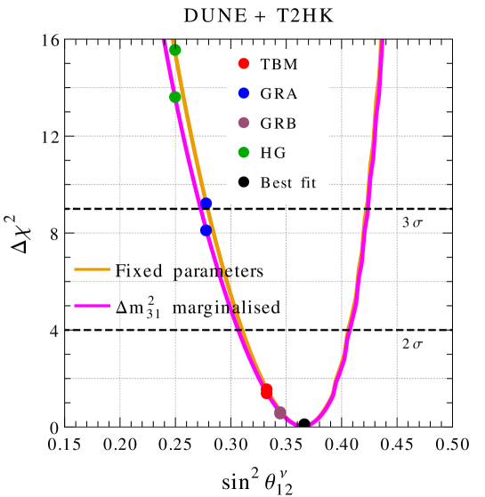
Figure 5: Compatibility between various symmetry forms and present best fit values of neutrino oscillation parameters in light of the prospective data from the combined DUNE + T2HK set-up. The black dot corresponds to $\sin^{2}\theta^{\nu}_{12}=0.364$ obtained from eq. (1.1) using the present best fit values of $\theta_{12}$, $\theta_{13}$, $\theta_{23}$, and $\delta_{\mathrm{CP}}$. The coloured dots correspond to the values of $\sin^{2}\theta^{\nu}_{12}$ for the TBM, GRA, GRB, and HG symmetry forms. We show the results for the two different cases: (i) fixed parameter scenario where all the oscillation parameters are kept fixed in the fit, and (ii) we only marginalise over $\Delta m_{31}^{2}$ in the fit in its present 3$\sigma$ allowed range.

In this appendix, we give Fig. 5 to show the impact of the present 3$\sigma$ uncertainty on $\Delta m_{31}^{2}$ while testing the compatibility between the considered symmetry forms and present oscillation data. In Fig. 5, we show the potential of the combined DUNE + T2HK set-up for the two different cases: (i) fixed parameter scenario where we keep all the oscillation parameters fixed at their benchmark values in the fit, and (ii) we only marginalise over $\Delta m_{31}^{2}$ in the fit in its present 3$\sigma$ allowed range. The fixed parameter curve is exactly similar to what we have already presented in Fig. 1 for the combined DUNE + T2HK set-up. For the GRB and TBM schemes, we do not see much difference between the fixed parameter case and the case where we marginalise over $\Delta m_{31}^{2}$ in the fit. For the GRA (HG) symmetry form, $\Delta\chi^{2}$ gets reduced by $\sim$ 11% (13%), when we marginalise over $\Delta m_{31}^{2}$ instead of keeping it fixed in the fit.

Appendix C Agreement between Various Mixing Schemes and Oscillation Data in $\boldsymbol{(\sin^{2}\theta_{23}^{\rm true},\delta_{\mathrm{CP}}^{\rm true})}$ Plane

Here we will see which regions of the parameter space in the plane of true values of $\sin^{2}\theta_{23}$ and $\delta_{\mathrm{CP}}$ will be compatible at less than $3\sigma$ C.L. for each symmetry form of interest, if that form is realised in Nature. To this aim, for each symmetry form (fixed $\theta^{\nu}_{12}$), we calculate $\delta_{\mathrm{CP}}$ using eq. (1.1) with the test values of the mixing angles $\theta_{ij}^{\rm test}$. Then, we marginalise $\Delta\chi^{2}$ over $\theta_{ij}^{\rm test}$ for given true values $\theta_{23}^{\rm true}$ and $\delta_{\mathrm{CP}}^{\rm true}$. The coloured bands in Fig. 6 represent potentially true values of $\delta_{\mathrm{CP}}$ as well as $\sin^{2}\theta_{23}$ with which the form under consideration is compatible at $1\sigma$, $2\sigma$, $3\sigma$ confidence levels in the context of DUNE, T2HK and their combination. If the true value of $\delta_{\mathrm{CP}}$ turned out to lie outside these bands, this would imply that the given symmetry form is disfavoured at more than $3\sigma$ C.L. For all the symmetry forms, a significant part of the parameter space gets disfavoured at more than $3\sigma$.

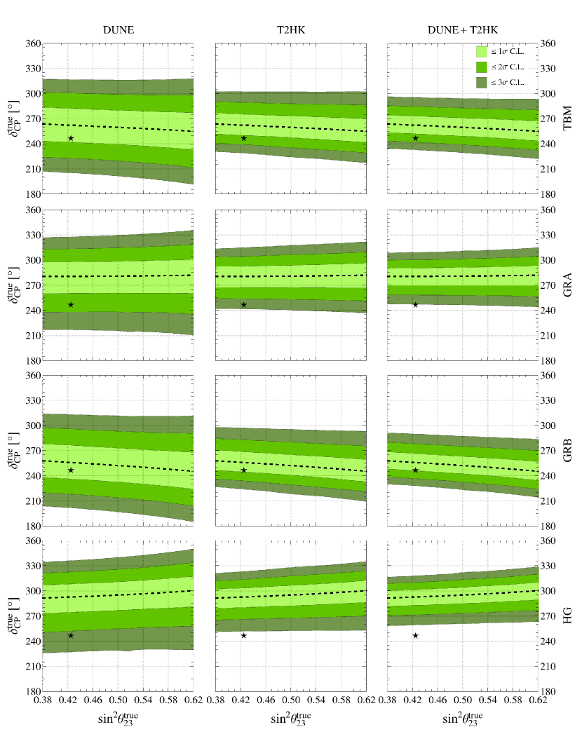
Figure 6: Compatibility of various symmetry forms with any potentially true values of $\sin^{2}\theta_{23}$ and $\delta_{\mathrm{CP}}$ in the context of DUNE (left panels), T2HK (middle panels), and DUNE + T2HK (right panels). For a given symmetry form (fixed $\theta^{\nu}_{12}$), the black dashed line has been obtained using eq. (1.1) and fixing $\theta_{12}$ and $\theta_{13}$ to their NO best fit values. The star indicates the present best fit values for NO as given in Table 1. For all the symmetry forms, a significant part of the parameter space gets disfavoured at more than $3\sigma$ C.L. for DUNE + T2HK.

For each symmetry form, the black dashed line has been obtained using eq. (1.1) with $\theta_{12}$ and $\theta_{13}$ fixed to their NO best fit values. Note that a given symmetry form is well compatible with any point close to this line. The star denotes the present best fit values of $\sin^{2}\theta_{23}$ and $\delta_{\mathrm{CP}}$ for the NO spectrum as given in Table 1, namely, $(\sin^{2}\theta_{23},\delta_{\mathrm{CP}})=(0.425,248\degree)$. As we can see from the right panels of Fig. 6, i.e., in the context of DUNE + T2HK, the HG (GRA) form is disfavoured at more than (precisely) $3\sigma$ C.L., while the GRB and TBM forms are compatible with the star at $1\sigma$ and $2\sigma$, respectively. If the star moves in the future to a different point, we will immediately conclude which symmetry forms are (dis)favoured. Let us assume, e.g., that the future best fit values are $(\sin^{2}\theta_{23},\delta_{\mathrm{CP}})=(0.58,300\degree)$. Then, in the context of DUNE + T2HK, the GRB and TBM forms would be disfavoured at more than $3\sigma$, while the HG (GRA) symmetry form would be compatible with this hypothetical position of the star at $1\sigma$ ($2\sigma$) confidence level.

Finally, we would like to notice the compatibility between this figure and the numbers in Table 5. Let us consider an example, in which GRB is the true form and HG is tested against it. In this case, from Table 5, we read the C.L. at which these two symmetry forms can be distinguished by DUNE + T2HK, namely, $3.3\sigma$. We recall that the results in this table have been obtained assuming the current best fit values of the mixing angles to be their true values. Thus, for GRB we have $(\sin^{2}\theta_{23},\delta_{\mathrm{CP}})=(0.425,256\degree)$, which are the true values of these parameters in the case under consideration. Now, we put this point on the right bottom panel of Fig. 6, corresponding to the HG symmetry form for DUNE + T2HK, and find that this point falls just outside the dark green band representing $\delta_{\mathrm{CP}}$ values compatible with the HG form at $3\sigma$ C.L. It means that if $\delta_{\mathrm{CP}}$ predicted by GRB together with the present best fit values of $\theta_{23}$, $\theta_{12}$, and $\theta_{13}$ are realised in Nature, then the HG symmetry form will be disfavoured by DUNE + T2HK at $>3\sigma$. The same message is conveyed from Table 5 as well.

References

- [1] K. Nakamura and S. T. Petcov, Neutrino Mass, Mixing, and Oscillations, in Particle Data Group Collaboration, C. Patrignani et al., Review of Particle Physics, Chin. Phys. C 40 (2016) 100001.
- [2] I. Esteban, M. C. Gonzalez-Garcia, M. Maltoni, I. Martinez-Soler and T. Schwetz, Updated fit to three neutrino mixing: exploring the accelerator-reactor complementarity, JHEP 01 (2017) 087, [1611.01514].
- [3] F. Capozzi, E. Di Valentino, E. Lisi, A. Marrone, A. Melchiorri and A. Palazzo, Global constraints on absolute neutrino masses and their ordering, Phys. Rev. D 95 (2017) 096014, [1703.04471].
- [4] P. F. de Salas, D. V. Forero, C. A. Ternes, M. Tortola and J. W. F. Valle, Status of neutrino oscillations 2017, 1708.01186.
- [5] G. Altarelli and F. Feruglio, Discrete Flavor Symmetries and Models of Neutrino Mixing, Rev. Mod. Phys. 82 (2010) 2701–2729, [1002.0211].
- [6] H. Ishimori, T. Kobayashi, H. Ohki, Y. Shimizu, H. Okada and M. Tanimoto, Non-Abelian Discrete Symmetries in Particle Physics, Prog. Theor. Phys. Suppl. 183 (2010) 1–163, [1003.3552].
- [7] S. F. King and C. Luhn, Neutrino Mass and Mixing with Discrete Symmetry, Rept. Prog. Phys. 76 (2013) 056201, [1301.1340].
- [8] S. T. Petcov, Predicting the values of the leptonic CP violation phases in theories with discrete flavour symmetries, Nucl. Phys. B 892 (2015) 400–428, [1405.6006].
- [9] I. Girardi, S. T. Petcov and A. V. Titov, Determining the Dirac CP Violation Phase in the Neutrino Mixing Matrix from Sum Rules, Nucl. Phys. B 894 (2015) 733–768, [1410.8056].
- [10] I. Girardi, S. T. Petcov and A. V. Titov, Predictions for the Dirac CP Violation Phase in the Neutrino Mixing Matrix, Int. J. Mod. Phys. A 30 (2015) 1530035, [1504.02402].
- [11] I. Girardi, S. T. Petcov and A. V. Titov, Predictions for the Leptonic Dirac CP Violation Phase: a Systematic Phenomenological Analysis, Eur. Phys. J. C 75 (2015) 345, [1504.00658].
- [12] I. Girardi, S. T. Petcov, A. J. Stuart and A. V. Titov, Leptonic Dirac CP Violation Predictions from Residual Discrete Symmetries, Nucl. Phys. B 902 (2016) 1–57, [1509.02502].
- [13] D. Marzocca, S. T. Petcov, A. Romanino and M. C. Sevilla, Nonzero from Charged Lepton Corrections and the Atmospheric Neutrino Mixing Angle, JHEP 05 (2013) 073, [1302.0423].
- [14] M. Tanimoto, Neutrinos and flavor symmetries, AIP Conf. Proc. 1666 (2015) 120002.
- [15] P. Ballett, S. F. King, C. Luhn, S. Pascoli and M. A. Schmidt, Testing atmospheric mixing sum rules at precision neutrino facilities, Phys. Rev. D 89 (2014) 016016, [1308.4314].
- [16] S.-F. Ge, D. A. Dicus and W. W. Repko, Symmetry Prediction for the Leptonic Dirac CP Phase, Phys. Lett. B 702 (2011) 220–223, [1104.0602].
- [17] S.-F. Ge, D. A. Dicus and W. W. Repko, Residual Symmetries for Neutrino Mixing with a Large and Nearly Maximal , Phys. Rev. Lett. 108 (2012) 041801, [1108.0964].
- [18] S. Antusch, S. F. King, C. Luhn and M. Spinrath, Trimaximal mixing with predicted from a new type of constrained sequential dominance, Nucl. Phys. B 856 (2012) 328–341, [1108.4278].
- [19] A. D. Hanlon, S.-F. Ge and W. W. Repko, Phenomenological consequences of residual and symmetries, Phys. Lett. B 729 (2014) 185–191, [1308.6522].
- [20] G. C. Branco, L. Lavoura and M. N. Rebelo, Majorana Neutrinos and CP Violation in the Leptonic Sector, Phys. Lett. B 180 (1986) 264–268.
- [21] F. Feruglio, C. Hagedorn and R. Ziegler, Lepton Mixing Parameters from Discrete and CP Symmetries, JHEP 07 (2013) 027, [1211.5560].
- [22] M. Holthausen, M. Lindner and M. A. Schmidt, CP and Discrete Flavour Symmetries, JHEP 04 (2013) 122, [1211.6953].
- [23] S. M. Bilenky, J. Hosek and S. T. Petcov, On Oscillations of Neutrinos with Dirac and Majorana Masses, Phys. Lett. B 94 (1980) 495–498.
- [24] I. Girardi, A. Meroni, S. T. Petcov and M. Spinrath, Generalised geometrical CP violation in a lepton flavour model, JHEP 02 (2014) 050, [1312.1966].
- [25] P. Ballett, S. Pascoli and J. Turner, Mixing angle and phase correlations from A5 with generalized CP and their prospects for discovery, Phys. Rev. D 92 (2015) 093008, [1503.07543].
- [26] J. Turner, Predictions for leptonic mixing angle correlations and nontrivial Dirac CP violation from A5 with generalized CP symmetry, Phys. Rev. D 92 (2015) 116007, [1507.06224].
- [27] I. Girardi, S. T. Petcov and A. V. Titov, Predictions for the Majorana CP Violation Phases in the Neutrino Mixing Matrix and Neutrinoless Double Beta Decay, Nucl. Phys. B 911 (2016) 754–804, [1605.04172].
- [28] J.-N. Lu and G.-J. Ding, Alternative Schemes of Predicting Lepton Mixing Parameters from Discrete Flavor and CP Symmetry, Phys. Rev. D 95 (2017) 015012, [1610.05682].
- [29] J. T. Penedo, S. T. Petcov and A. V. Titov, Neutrino mixing and leptonic CP violation from S4 flavour and generalised CP symmetries, JHEP 12 (2017) 022, [1705.00309].
- [30] P. Ballett, S. F. King, C. Luhn, S. Pascoli and M. A. Schmidt, Testing solar lepton mixing sum rules in neutrino oscillation experiments, JHEP 12 (2014) 122, [1410.7573].
- [31] M. Sruthilaya, S. C, K. N. Deepthi and R. Mohanta, Predicting Leptonic CP phase by considering deviations in charged lepton and neutrino sectors, New J. Phys. 17 (2015) 083028, [1408.4392].
- [32] S. T. Petcov, On Pseudo-Dirac Neutrinos, Neutrino Oscillations and Neutrinoless Double beta Decay, Phys. Lett. B 110 (1982) 245–249.
- [33] F. Vissani, A Study of the scenario with nearly degenerate Majorana neutrinos, hep-ph/9708483.
- [34] V. D. Barger, S. Pakvasa, T. J. Weiler and K. Whisnant, Bimaximal mixing of three neutrinos, Phys. Lett. B 437 (1998) 107–116, [hep-ph/9806387].
- [35] A. J. Baltz, A. S. Goldhaber and M. Goldhaber, The Solar neutrino puzzle: An Oscillation solution with maximal neutrino mixing, Phys. Rev. Lett. 81 (1998) 5730–5733, [hep-ph/9806540].
- [36] P. F. Harrison, D. H. Perkins and W. G. Scott, Tri-bimaximal mixing and the neutrino oscillation data, Phys. Lett. B 530 (2002) 167, [hep-ph/0202074].
- [37] P. F. Harrison and W. G. Scott, Symmetries and generalizations of tri - bimaximal neutrino mixing, Phys. Lett. B 535 (2002) 163–169, [hep-ph/0203209].
- [38] Z.-z. Xing, Nearly tri bimaximal neutrino mixing and CP violation, Phys. Lett. B 533 (2002) 85–93, [hep-ph/0204049].
- [39] X. G. He and A. Zee, Some simple mixing and mass matrices for neutrinos, Phys. Lett. B 560 (2003) 87–90, [hep-ph/0301092].
- [40] L. Wolfenstein, Oscillations Among Three Neutrino Types and CP Violation, Phys. Rev. D 18 (1978) 958–960.
- [41] A. Datta, F.-S. Ling and P. Ramond, Correlated hierarchy, Dirac masses and large mixing angles, Nucl. Phys. B 671 (2003) 383–400, [hep-ph/0306002].
- [42] Y. Kajiyama, M. Raidal and A. Strumia, The Golden ratio prediction for the solar neutrino mixing, Phys. Rev. D 76 (2007) 117301, [0705.4559].
- [43] L. L. Everett and A. J. Stuart, Icosahedral () Family Symmetry and the Golden Ratio Prediction for Solar Neutrino Mixing, Phys. Rev. D 79 (2009) 085005, [0812.1057].
- [44] W. Rodejohann, Unified Parametrization for Quark and Lepton Mixing Angles, Phys. Lett. B 671 (2009) 267–271, [0810.5239].
- [45] A. Adulpravitchai, A. Blum and W. Rodejohann, Golden Ratio Prediction for Solar Neutrino Mixing, New J. Phys. 11 (2009) 063026, [0903.0531].
- [46] C. H. Albright, A. Dueck and W. Rodejohann, Possible Alternatives to Tri-bimaximal Mixing, Eur. Phys. J. C 70 (2010) 1099–1110, [1004.2798].
- [47] J. E. Kim and M.-S. Seo, Quark and lepton mixing angles with a dodeca-symmetry, JHEP 02 (2011) 097, [1005.4684].
- [48] P. Ballett, S. F. King, S. Pascoli, N. W. Prouse and T. Wang, Precision neutrino experiments vs the Littlest Seesaw, JHEP 03 (2017) 110, [1612.01999].
- [49] S. S. Chatterjee, P. Pasquini and J. W. F. Valle, Probing atmospheric mixing and leptonic CP violation in current and future long baseline oscillation experiments, Phys. Lett. B 771 (2017) 524–531, [1702.03160].
- [50] S. S. Chatterjee, M. Masud, P. Pasquini and J. W. F. Valle, Cornering the revamped BMV model with neutrino oscillation data, Phys. Lett. B 774 (2017) 179–182, [1708.03290].
- [51] P. Pasquini, Reactor and Atmospheric Neutrino Mixing Angles’ Correlation as a Probe for New Physics, 1708.04294.
- [52] S. Pascoli and T. Schwetz, Prospects for neutrino oscillation physics, Adv. High Energy Phys. 2013 (2013) 503401.
- [53] DUNE Collaboration, R. Acciarri et al., Long-Baseline Neutrino Facility (LBNF) and Deep Underground Neutrino Experiment (DUNE) Conceptual Design Report, Volume 1: The LBNF and DUNE Projects, 1601.05471.
- [54] DUNE Collaboration, R. Acciarri et al., Long-Baseline Neutrino Facility (LBNF) and Deep Underground Neutrino Experiment (DUNE) Conceptual Design Report, Volume 2: The Physics Program for DUNE at LBNF, 1512.06148.
- [55] DUNE Collaboration, J. Strait et al., Long-Baseline Neutrino Facility (LBNF) and Deep Underground Neutrino Experiment (DUNE) Conceptual Design Report, Volume 3: Long-Baseline Neutrino Facility for DUNE, 1601.05823.
- [56] DUNE Collaboration, R. Acciarri et al., Long-Baseline Neutrino Facility (LBNF) and Deep Underground Neutrino Experiment (DUNE) Conceptual Design Report, Volume 4: The DUNE Detectors at LBNF, 1601.02984.
- [57] LBNE Collaboration, C. Adams et al., Scientific Opportunities with the Long-Baseline Neutrino Experiment, 1307.7335.
- [58] S. K. Agarwalla, T. Li and A. Rubbia, An Incremental approach to unravel the neutrino mass hierarchy and CP violation with a long-baseline Superbeam for large , JHEP 05 (2012) 154, [1109.6526].
- [59] Mary Bishai. Private communication, 2012.
- [60] K. Abe, T. Abe, H. Aihara, Y. Fukuda, Y. Hayato et al., Letter of Intent: The Hyper-Kamiokande Experiment — Detector Design and Physics Potential —, 1109.3262.
- [61] Hyper-Kamiokande Working Group Collaboration, K. Abe et al., A Long Baseline Neutrino Oscillation Experiment Using J-PARC Neutrino Beam and Hyper-Kamiokande, 1412.4673.
- [62] Hyper-Kamiokande Proto Collaboration, K. Abe et al., Physics potential of a long-baseline neutrino oscillation experiment using a J-PARC neutrino beam and Hyper-Kamiokande, PTEP 2015 (2015) 053C02, [1502.05199].
- [63] Hyper-Kamiokande Proto Collaboration, K. Abe et al., Physics Potentials with the Second Hyper-Kamiokande Detector in Korea, 1611.06118.
- [64] M. D. Messier, Evidence for neutrino mass from observations of atmospheric neutrinos with Super-Kamiokande, .
- [65] E. Paschos and J. Yu, Neutrino interactions in oscillation experiments, Phys. Rev. D 65 (2002) 033002, [hep-ph/0107261].
- [66] Geralyn Zeller. Private communication, 2012.
- [67] R. Petti and G. Zeller, “Nuclear Effects in Water vs. Argon.”
- [68] A. Dziewonski and D. Anderson, Preliminary reference Earth model, Physics of the Earth and Planetary Interiors 25 (1981) 297–356.
- [69] P. Huber, M. Lindner and W. Winter, Simulation of long-baseline neutrino oscillation experiments with GLoBES (General Long Baseline Experiment Simulator), Comput. Phys. Commun. 167 (2005) 195, [hep-ph/0407333].
- [70] P. Huber, J. Kopp, M. Lindner, M. Rolinec and W. Winter, New features in the simulation of neutrino oscillation experiments with GLoBES 3.0: General Long Baseline Experiment Simulator, Comput. Phys. Commun. 177 (2007) 432–438, [hep-ph/0701187].
- [71] S. K. Agarwalla, S. Prakash and S. Uma Sankar, Exploring the three flavor effects with future superbeams using liquid argon detectors, JHEP 03 (2014) 087, [1304.3251].
- [72] P. Ballett, S. F. King, S. Pascoli, N. W. Prouse and T. Wang, Sensitivities and synergies of DUNE and T2HK, Phys. Rev. D 96 (2017) 033003, [1612.07275].
- [73] Hyper-Kamiokande Proto Collaboration, M. Yokoyama, The Hyper-Kamiokande Experiment, in Proceedings, Prospects in Neutrino Physics (NuPhys2016): London, UK, December 12-14, 2016, 2017. 1705.00306.
- [74] E. K. Akhmedov, R. Johansson, M. Lindner, T. Ohlsson and T. Schwetz, Series expansions for three flavor neutrino oscillation probabilities in matter, JHEP 04 (2004) 078, [hep-ph/0402175].
- [75] JUNO Collaboration, F. An et al., Neutrino Physics with JUNO, J. Phys. G 43 (2016) 030401, [1507.05613].
- [76] Daya Bay Collaboration, J. Ling, Precision Measurement of and from Daya Bay, PoS ICHEP2016 (2016) 467.
- [77] P. Huber, M. Lindner and W. Winter, Superbeams versus neutrino factories, Nucl. Phys. B 645 (2002) 3–48, [hep-ph/0204352].
- [78] G. Fogli, E. Lisi, A. Marrone, D. Montanino, A. Palazzo et al., Solar neutrino oscillation parameters after first KamLAND results, Phys. Rev. D 67 (2003) 073002, [hep-ph/0212127].
- [79] M. Blennow, P. Coloma, P. Huber and T. Schwetz, Quantifying the sensitivity of oscillation experiments to the neutrino mass ordering, JHEP 03 (2014) 028, [1311.1822].