Wirelessly Powered Crowd Sensing: Joint Power Transfer, Sensing, Compression, and Transmission

Xiaoyang Li, Changsheng You, Sergey Andreev, Yi Gong, and Kaibin Huang This work was supported in part by Hong Kong Research Grants Council under the Grants 17209917 and 17259416, and Natural Science Foundation of Guangdong Province under Grant 2015A030313844. X. Li, C. You, and K. Huang are with the Dept. of EEE at The University of Hong Kong, Hong Kong (e-mail: lixy@eee.hku.hk, csyou@eee.hku.hk; huangkb@eee.hku.hk). X. Li is also with the Dept. of EEE at Southern University of Science and Technology, Shenzhen, China. S. Andreev is with the Laboratory of Electronics and Communications Engineering, Tampere University of Technology, Finland (e-mail: sergey.andreev@tut.fi). Y. Gong is with the Dept. of EEE at Southern University of Science and Technology, Shenzhen, China (e-mail: gongy@sustc.edu.cn).
Abstract

Leveraging massive numbers of sensors in user equipment as well as opportunistic human mobility, mobile crowd sensing (MCS) has emerged as a powerful paradigm, where prolonging battery life of constrained devices and motivating human involvement are two key design challenges. To address these, we envision a novel framework, named wirelessly powered crowd sensing (WPCS), which integrates MCS with wireless power transfer (WPT) for supplying the involved devices with extra energy and thus facilitating user incentivization. This paper considers a multiuser WPCS system where an access point (AP) transfers energy to multiple mobile sensors (MSs), each of which performs data sensing, compression, and transmission. Assuming lossless (data) compression, an optimization problem is formulated to simultaneously maximize data utility and minimize energy consumption at the operator side, by jointly controlling wireless-power allocation at the AP as well as sensing-data sizes, compression ratios, and sensor-transmission durations at the MSs. Given fixed compression ratios, the proposed optimal power allocation policy has the threshold-based structure with respect to a defined crowd-sensing priority function for each MS depending on both the operator configuration and the MS information. Further, for fixed sensing-data sizes, the optimal compression policy suggests that compression can reduce the total energy consumption at each MS only if the sensing-data size is sufficiently large. Our solution is also extended to the case of lossy compression, while extensive simulations are offered to confirm the efficiency of the contributed mechanisms.

I Introduction

The unprecedented growth of the Internet of Things (IoT) applications for Smart Cities fuels the deployment of billions of wireless IoT devices that help automate a wide range of services, such as temperature measurement, pollution assessment, traffic monitoring, and public-safety surveillance. However, traditional wireless sensor networking (WSN) solutions are limited in their coverage and scalability, as well as suffer from high maintenance costs [1]. Recently, leveraging massive numbers of sensors in user handheld and wearable equipment led to the emergence of mobile crowd sensing (MCS), which is becoming a new paradigm that involves humans as part of the sensing infrastructure [2]. The key MCS challenges are prolonging device battery life and facilitating human engagement. These can be tackled by leveraging wireless power transfer (WPT) techniques as a user incentive for charging mobile sensors (MSs) within our proposed framework of wirelessly powered crowd sensing (WPCS) [3].

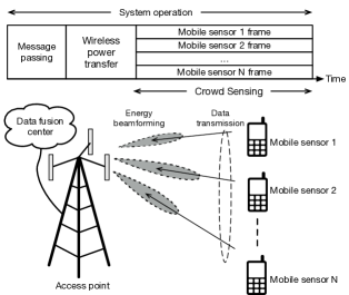
In this work, we consider a multiuser WPCS system in Fig. 1, which comprises an operator-deployed access point (AP) that transfers energy to multiple MSs. To optimize the operator’s reward, we design a set of efficient control policies for maximizing data utility and minimizing energy consumption simultaneously.

I-A Mobile Crowd Sensing

The consideration of MCS for IoT in Smart Cities has motivated research on advanced technologies that go beyond conventional WSNs, such as personal location-based systems, trusted sensing platforms, and people-centric sensing applications [2]. A key MCS design issue is how to involve people into collaborate sensing, as users may not be willing to contribute if the associated energy costs are high. There are two approaches to address this issue, known as opportunistic and participatory sensing [4, 5]. The former assumes that applications may run in the background and opportunistically collect data without user attention. The latter requires users to consciously participate in sensing activities and timely transmit the operator-requested data. However, this may consume significant device resources (i.e., battery and computing power), and it is essential to design incentivization mechanisms that compensate for the costs of participation [6, 7, 8].
Refer to caption
Figure 1: Our considered multiuser WPCS system.

Specifically, inspired by the location-based games, entertainment as an incentive can enrich the experience of participants who collect e.g., geographic data on user preferences and interests. Service as an incentive is another widely-recognized mechanism. A typical example here is traffic monitoring, wherein users provide real-time traffic information (e.g., on road congestion levels) and in return receive timely services, such as accurate route planning. Finally, money as an incentive is an intuitive method that interprets sensed data as goods for gaining profit. Accordingly, an auction scheme for MCS named reverse auction was proposed in [7], where the sellers (i.e., participants) submit their bidding prices to the buyer (i.e., operator) to compete for the data sensing activities. Further, the operator selects a subset of MSs for crowd sensing operation and determines individual payments.

In [8], the authors designed an alternative framework by utilizing Stackelberg game for monetary incentivization. The operator and the MSs negotiate in a two-stage manner to achieve the Stackelberg equilibrium: first the operator announces the payments and then each MS decides on whether to participate. Here, incentive allocation in multiuser MCS systems depends on data quality of each user, which has been investigated in [9, 10]. In particular, the user data quality was estimated in [9] by using unsupervised learning techniques for characterizing long-term reputation. For privacy management, inverse correlation between the service quality and the privacy level was determined in [10] from the perspective of data analytics. Despite these substantial efforts, the issue of energy consumption at the MSs is not yet resolved. The proposed work addresses it by relying on advanced WPT techniques as well as contributes the first theoretical resource-allocation design of trading energy for data, which we envisioned in [3].

I-B Wirelessly Powered Communication and Sensing

Designed originally for point-to-point power transmission, the WPT technology has already comprised advanced techniques from inductive coupling and electromagnetic radiation [11, 12]. According to [13], the power to be wirelessly transferred is on the level of micro-watt, thus WPT is mostly applied for the ultra-dense small cell networks. Further integration of information and power transfer gave rise to the emerging field of simultaneous wireless information and power transmission (SWIPT) [14]. Multiple studies focused on applying SWIPT to a variety of communication systems and networks, including multiple-input-multiple-output (MIMO) communications [14, 15], two-way transmissions [16], relaying [17, 18, 19], orthogonal frequency-division multiple access (OFDMA) transmissions [20], and cognitive networking [21, 22], among others. Further design efforts tailored it for practical setups by accounting for channel state information [23] and quality of service [24]. Recently, WPT was considered for unmanned aerial vehicles [25] and mobile-edge computing networks [26] for powering computation offloading in energy-constrained devices.

Another important application of WPT is in sensing systems, where the MSs have a limited energy storage due to their compact form-factor, but are expected to perform sophisticated sensing tasks cooperatively. Powering these sensors is challenging, since frequent battery recharging/replacement is impractical if not impossible. Recent breakthroughs in WPT techniques offer a viable solution by powering MSs with energy beamforming [27, 28, 29, 30, 31]. Specifically, a multi-antenna wirelessly powered sensor networking (WPSN) testbed has been developed in [28], where a power beacon transfers energy to a sensor node via an adaptive energy-beamforming scheme.

For multiple WPSN sensors, efficient design of energy beamforming is much more convoluted. In [29], accounting for practical sensing and circuit power consumption at MSs, the authors proposed a collaborative energy-beamforming scheme for powering a cluster of sensors to transfer data by using distributed information beamforming. Cooperative sensing was further addressed in [30], where clusters of sensors forward their information by utilizing relay and SWIPT techniques. Finally, for low-complexity passive backscatter sensors, a novel architecture for large-scale WPSN systems was recently proposed in [31], where the sensors are powered by distributed power beacons. However, the existing literature concentrates on optimizing WPT efficiency to improve the sensing-and-communication throughput, but disregards the design of user incentivization and operator reward schemes. In this work, we bridge this gap by integrating WPT with MCS to facilitate human involvement into collective sensing activities, thus simultaneously maximizing data utility and minimizing energy consumption at the operator side.

I-C Contributions and Organization

In this work, by leveraging the potential of WPT for powering MSs and motivating MCS, we aim at addressing the following two key issues.

  • The first one is how to incentivize and select MSs for crowd-sensing operation. This includes designing a new incentivization approach that can trade energy for data depending on the data utility at different MSs. An optimized sensor selection policy needs to be developed at the operator to select a set of sensors to participate in the MCS for the maximum reward.

  • The second one is how to jointly control wireless-power allocation, data sensing, compression, and transmission at the selected MSs. This requires the operator to allocate wireless power for improved energy supply of each MS, while the MSs should employ energy-efficient sensing, compression, and transmission policies to minimize the energy consumption.

To account for these two considerations, this paper addresses a multiuser WPCS system controlled by an operator and comprising a multiple-antenna AP that transfers energy to multiple single-antenna MSs. Each MS accumulates part of such energy as a reward and utilizes the rest to conduct the MCS tasks, including sensing, data compression, and transmission of compressed data to the AP. We consider both lossless and lossy (data) compression as well as design a joint control policy for maximizing the data utility and minimizing the energy consumption at the AP simultaneously. The main contributions of this work are summarized as follows.

  • Problem Formulation and Iterative Solution: For lossless compression, we formulate an optimization problem for simultaneously maximizing data utility and minimizing energy consumption at the operator. An iterative solution that reaches the local optimum is then proposed for a joint optimization of power allocation, sensing, compression, and transmission.

  • Joint Optimization of Power Allocation, Sensing, and Transmission: Given fixed compression ratios, the considered non-convex problem is reduced to a convex formulation. We first derive a semi-closed form expression for the optimal sensor-transmission duration. The results are used for deriving the optimal wireless-power allocation and sensing-data sizes.

  • Joint Optimization of Compression and Transmission: Given fixed sensing-data sizes, the sensor-transmission durations and compression ratios are optimized for minimizing energy consumption at the operator. The derived optimal policy suggests that the MSs should perform data compression only if the sensing-data size exceeds a certain threshold.

  • Optimal Control for Lossy Compression: The proposed solution is further extended to lossy compression, while the optimization problem is modified to account for the respective data utility degradation. Given fixed compression ratios, the corresponding approach is similar to the lossless case. For the optimization of compression to preserve the data utility, we further optimize both the sensing-data sizes and the compression ratios at the MSs.

The rest of this paper is organized as follows. The system model is introduced in Section II. Section III studies efficient joint control in the WPCS system based on lossless compression. In Section IV, this approach is extended for the system with lossy compression. Simulation results are offered in Section V, followed by the conclusions in Section VI.

II System Model

Consider a multiuser WPCS system shown in Fig. 1 and comprising multiple single-antenna MSs together with one multi-antenna AP. The model of system operation is described in below sub-sections.

II-A WPCS Operation

We focus on a particular fixed time window for crowd-sensing, which is divided into three phases: message passing, WPT, and crowd sensing (see Fig. 1).

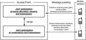
Consider the message-passing phase. Each sensor feeds back to the AP its parameters including the effective channel power gain, sensing, and compression power. Given the knowledge of all sensor parameters, the AP jointly optimizes the power allocation for WPT and sensor operations (namely, data sensing, compression, and transmission). The objective is to simultaneously maximize the data utility and minimize the energy consumption (see the performance metrics in the sequel). Subsequently, the AP informs individual sensors on their allocated power, optimal compression ratios, sensing-data sizes, and time partitions for sensing, compression, and transmission. The power consumption at the AP for transmitting these control parameters is negligible due to their small data sizes.

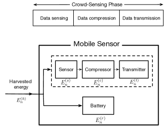
Further, in the WPT phase, the AP employs an antenna array to beam energy to the MSs as an incentive for sensing (see Fig. 1). Upon harvesting energy, each MS stores a part of it as a reward and applies the rest to operate the sensing tasks, including sensing, data compression, and transmission of compressed data to the AP.

Finally, in the crowd-sensing phase, the sensors simultaneously perform data sensing, compression, and transmission based on the settings determined by the AP in the message-passing phase. Parallel data collection is enabled via transmissions over orthogonal channels as allocated by the AP to the sensors based on OFDMA. The time duration for crowd sensing, denoted as T𝑇T, is divided into three slots with adjustable durations tn(s)superscriptsubscript𝑡𝑛𝑠t_{n}^{(s)}, tn(c)superscriptsubscript𝑡𝑛𝑐t_{n}^{(c)}, and tnsubscript𝑡𝑛t_{n}, which are used for sensing, compression, and transmission, respectively. This introduces the following constraint:

(Time constraint)tn(s)+tn(c)+tnT.(Time constraint)superscriptsubscript𝑡𝑛𝑠superscriptsubscript𝑡𝑛𝑐subscript𝑡𝑛𝑇\text{(Time constraint)}\quad t_{n}^{(s)}+t_{n}^{(c)}+t_{n}\leq T. (1)

II-B Model of Wireless Power Transfer

In the WPT phase with a fixed duration of T0subscript𝑇0T_{0} (seconds), the AP transfers energy simultaneously to N𝑁N MSs by pointing N𝑁N radio beams to the corresponding MSs. Let gnsubscript𝑔𝑛g_{n} denote the effective channel power gain between the AP and MS n𝑛n using energy beamforming, while Pnsubscript𝑃𝑛P_{n} is the transmission power of the corresponding beam. The AP transmission power is assumed to be fixed and represented by P0subscript𝑃0P_{0}, thus resulting in the following constraint:

(Power constraint)n=1NPnP0.(Power constraint)superscriptsubscript𝑛1𝑁subscript𝑃𝑛subscript𝑃0\text{(Power constraint)}\quad\sum_{n=1}^{N}P_{n}\leq P_{0}. (2)

The energy transferred from the AP to MS n𝑛n, denoted by En(h)(Pn)superscriptsubscript𝐸𝑛subscript𝑃𝑛E_{n}^{(h)}(P_{n}), is En(h)(Pn)=ηgnPnT0superscriptsubscript𝐸𝑛subscript𝑃𝑛𝜂subscript𝑔𝑛subscript𝑃𝑛subscript𝑇0E_{n}^{(h)}(P_{n})=\eta g_{n}P_{n}T_{0}, where the constant 0<η<10𝜂10<\eta<1 represents the energy conversion efficiency.

Each of the sensors selected to participate in the crowd sensing stores a part of received energy as its reward. Let the reward energy at sensor n𝑛n, denoted by En(r)(n(s))superscriptsubscript𝐸𝑛𝑟superscriptsubscript𝑛𝑠E_{n}^{(r)}(\ell_{n}^{(s)}), be proportional to the size of sensing data, namely, En(r)(n(s))=qn(r)n(s)superscriptsubscript𝐸𝑛𝑟superscriptsubscript𝑛𝑠superscriptsubscript𝑞𝑛𝑟superscriptsubscript𝑛𝑠E_{n}^{(r)}(\ell_{n}^{(s)})=q_{n}^{(r)}\ell_{n}^{(s)} with qn(r)superscriptsubscript𝑞𝑛𝑟q_{n}^{(r)} being a fixed scaling factor. The remaining energy, (En(h)En(r))superscriptsubscript𝐸𝑛superscriptsubscript𝐸𝑛𝑟\left(E_{n}^{(h)}-E_{n}^{(r)}\right), is consumed by the sensor operations, including sensing, compression, and transmission, where energy consumption is represented respectively by En(s)superscriptsubscript𝐸𝑛𝑠E_{n}^{(s)}, En(c)superscriptsubscript𝐸𝑛𝑐E_{n}^{(c)} and En(t)superscriptsubscript𝐸𝑛𝑡E_{n}^{(t)} as specified in the sequel. Based on the above discussion, each MS should satisfy the following energy constraint:

(Energy constraint)En(r)+En(s)+En(c)+En(t)ηgnPnT0.(Energy constraint)superscriptsubscript𝐸𝑛𝑟superscriptsubscript𝐸𝑛𝑠superscriptsubscript𝐸𝑛𝑐superscriptsubscript𝐸𝑛𝑡𝜂subscript𝑔𝑛subscript𝑃𝑛subscript𝑇0\text{(Energy constraint)}\leavevmode\nobreak\ E_{n}^{(r)}\!+\!E_{n}^{(s)}\!+\!E_{n}^{(c)}\!+\!E_{n}^{(t)}\!\leq\!\eta g_{n}P_{n}T_{0}. (3)
Refer to caption
Figure 2: MS architecture, operation, and energy consumption.

II-C Mobile-Sensor Model

At each MS, crowd sensing comprises three sequential operations: data sensing, data compression, and data transmission as shown in Fig. 2 and modeled as follows.

II-C1 Data sensing model

Consider MS n𝑛n. Let snsubscript𝑠𝑛s_{n} denote the output data rate. Given the sensing time-duration tn(s)superscriptsubscript𝑡𝑛𝑠t_{n}^{(s)}, the size of raw sensing data, denoted by n(s)superscriptsubscript𝑛𝑠\ell_{n}^{(s)} (in bits), is n(s)=sntn(s)superscriptsubscript𝑛𝑠subscript𝑠𝑛superscriptsubscript𝑡𝑛𝑠\ell_{n}^{(s)}=s_{n}t_{n}^{(s)}. Based on the data-sensing energy consumption model in [32], let qn(s)superscriptsubscript𝑞𝑛𝑠q_{n}^{(s)} denote the sensing energy consumption for generating 111-bit of data. The total energy consumption for sensing at MS n𝑛n, denoted as En(s)(n(s))superscriptsubscript𝐸𝑛𝑠superscriptsubscript𝑛𝑠E_{n}^{(s)}(\ell_{n}^{(s)}), is given as En(s)(n(s))=qn(s)n(s)superscriptsubscript𝐸𝑛𝑠superscriptsubscript𝑛𝑠superscriptsubscript𝑞𝑛𝑠superscriptsubscript𝑛𝑠E_{n}^{(s)}(\ell_{n}^{(s)})=q_{n}^{(s)}\ell_{n}^{(s)}.

II-C2 Data compression model

First, consider lossless compression of sensed data, for which the original data can be perfectly reconstructed from the compressed data. Relevant techniques include Huffman, run-length, and Lempel-Ziv encoding. It is assumed that all MSs deploy the same lossless compression method with the maximum compression ratio denoted as Rmaxsubscript𝑅maxR_{\rm{max}}, namely, the maximum ratio between the sizes of raw and compressed data. Let Rn[1,Rmax]subscript𝑅𝑛1subscript𝑅maxR_{n}\in[1,R_{\rm{max}}] denote the compression ratio chosen by MS n𝑛n. Then, the size of compressed data nsubscript𝑛\ell_{n} is given as n=n(s)/Rnsubscript𝑛superscriptsubscript𝑛𝑠subscript𝑅𝑛\ell_{n}=\ell_{n}^{(s)}/R_{n}. Note that in the current literature, there is still a lack of well-established models for the computation complexity of data compression. However, a tractable model can be inferred from the existing measurement results for Zlib compression [33]. Specifically, the required CPU cycles for compressing 111-bit of data can be approximated as an exponential function of the compression ratio Rnsubscript𝑅𝑛R_{n} as:

(Compression complexity)C(Rn,ϵ)=eϵRneϵ,(Compression complexity)𝐶subscript𝑅𝑛italic-ϵsuperscript𝑒italic-ϵsubscript𝑅𝑛superscript𝑒italic-ϵ\text{(Compression complexity)}\quad C(R_{n},\epsilon)=e^{\epsilon R_{n}}-e^{\epsilon}, (4)

where ϵitalic-ϵ\epsilon is a positive constant depending on the compression method. At Rn=1subscript𝑅𝑛1R_{n}=1, C(Rn,ϵ)=0𝐶subscript𝑅𝑛italic-ϵ0C(R_{n},\epsilon)=0, which corresponds to no compression. Let fnsubscript𝑓𝑛f_{n} denote the fixed CPU-cycle frequency at MS n𝑛n and tn(c)superscriptsubscript𝑡𝑛𝑐t_{n}^{(c)} is the compression time duration. Then, tn(c)=(n(s)C(Rn,ϵ))/fnsuperscriptsubscript𝑡𝑛𝑐superscriptsubscript𝑛𝑠𝐶subscript𝑅𝑛italic-ϵsubscript𝑓𝑛t_{n}^{(c)}=(\ell_{n}^{(s)}C(R_{n},\epsilon))/f_{n}. Following the practical model in [34], each CPU cycle consumes the energy of qn(c)=αfn2superscriptsubscript𝑞𝑛𝑐𝛼superscriptsubscript𝑓𝑛2q_{n}^{(c)}=\alpha f_{n}^{2}, where α𝛼\alpha is a constant determined by the circuits. The energy consumption for data compression at MS n𝑛n, denoted by En(c)(n(s),Rn)superscriptsubscript𝐸𝑛𝑐superscriptsubscript𝑛𝑠subscript𝑅𝑛E_{n}^{(c)}(\ell_{n}^{(s)},R_{n}), is given as En(c)(n(s),Rn)=qn(c)n(s)C(Rn,ϵ)superscriptsubscript𝐸𝑛𝑐superscriptsubscript𝑛𝑠subscript𝑅𝑛superscriptsubscript𝑞𝑛𝑐superscriptsubscript𝑛𝑠𝐶subscript𝑅𝑛italic-ϵE_{n}^{(c)}(\ell_{n}^{(s)},R_{n})=q_{n}^{(c)}\ell_{n}^{(s)}C(R_{n},\epsilon) with C(Rn,ϵ)𝐶subscript𝑅𝑛italic-ϵC(R_{n},\epsilon) in (4). It follows that

(Compression energy)En(c)(n(s),Rn)=qn(c)n(s)(eϵRneϵ).(Compression energy)superscriptsubscript𝐸𝑛𝑐superscriptsubscript𝑛𝑠subscript𝑅𝑛superscriptsubscript𝑞𝑛𝑐superscriptsubscript𝑛𝑠superscript𝑒italic-ϵsubscript𝑅𝑛superscript𝑒italic-ϵ\text{(Compression energy)}\leavevmode\nobreak\ E_{n}^{(c)}(\ell_{n}^{(s)},R_{n})\!=\!q_{n}^{(c)}\ell_{n}^{(s)}(e^{\epsilon R_{n}}\!-\!e^{\epsilon}).\! (5)

Further, consider lossy compression that achieves a higher compression ratio than its lossless counterpart at the cost of some information loss. Typical techniques involve data truncation after a transform (e.g., discrete cosine transform) or discarding the data immaterial for user perception. Our model of compression energy consumption follows that in (5) with the parameters {Rn,Rmax,ϵ}subscript𝑅𝑛subscript𝑅maxitalic-ϵ\{R_{n},R_{\rm{max}},\epsilon\} replaced by their counterparts for lossy compression {Rˇn,Rˇmax,ϵˇ}subscriptˇ𝑅𝑛subscriptˇ𝑅maxˇitalic-ϵ\{\check{R}_{n},\check{R}_{\rm{max}},\check{\epsilon}\}. The information loss can be measured with a quality factor, denoted by bn(0,1]subscript𝑏𝑛01b_{n}\in(0,1] and defined as the equivalent size of raw data for 111-bit of compressed data in terms of utility. The quality factor, however, has not been well-modeled in the existing literature. To address it, one tractable model can be inferred from the simulation results in [35], given by bn=1/Rˇnsubscript𝑏𝑛1subscriptˇ𝑅𝑛b_{n}=1/\sqrt{\check{R}_{n}}. Specifically, bn0subscript𝑏𝑛0b_{n}\to 0 when Rˇnsubscriptˇ𝑅𝑛\check{R}_{n}\to\infty, and bn1subscript𝑏𝑛1b_{n}\to 1 when Rˇn1subscriptˇ𝑅𝑛1\check{R}_{n}\to 1, which corresponds to no compression.

II-C3 Data transmission model

Each selected MS transmits its compressed data to the AP. Let Pn(t)superscriptsubscript𝑃𝑛𝑡P_{n}^{(t)} denote the transmission power and tnsubscript𝑡𝑛t_{n} is the transmission time duration. Assuming channel reciprocity, the achievable transmission rate (in bits/s), denoted by vnsubscript𝑣𝑛v_{n}, can be given as vn=n/tn=Blog2(1+gnPn(t)N0)subscript𝑣𝑛subscript𝑛subscript𝑡𝑛𝐵subscript21subscript𝑔𝑛superscriptsubscript𝑃𝑛𝑡subscript𝑁0v_{n}=\ell_{n}/t_{n}=B\log_{2}(1+\frac{g_{n}P_{n}^{(t)}}{N_{0}}), where B𝐵B is the bandwidth and N0subscript𝑁0N_{0} is the variance of complex-white-Gaussian noise. Hence, the transmission energy consumption denoted by En(t)(n)superscriptsubscript𝐸𝑛𝑡subscript𝑛E_{n}^{(t)}(\ell_{n}) follows: En(t)(n)=Pn(t)tn=tngnf(n/tn)superscriptsubscript𝐸𝑛𝑡subscript𝑛superscriptsubscript𝑃𝑛𝑡subscript𝑡𝑛subscript𝑡𝑛subscript𝑔𝑛𝑓subscript𝑛subscript𝑡𝑛E_{n}^{(t)}(\ell_{n})=P_{n}^{(t)}t_{n}=\dfrac{t_{n}}{g_{n}}f(\ell_{n}/t_{n}), where the function f(x)𝑓𝑥f(x) is defined as f(x)=N0(2xB1)𝑓𝑥subscript𝑁0superscript2𝑥𝐵1f(x)=N_{0}(2^{\frac{x}{B}}-1).

II-C4 Time and energy constraints (revisited)

Finally, based on the above models, the time constraint in (1) and energy constraint in (3) can be rewritten as

n(s)sn+n(s)C(Rn,ϵ)fn+tnT,superscriptsubscript𝑛𝑠subscript𝑠𝑛superscriptsubscript𝑛𝑠𝐶subscript𝑅𝑛italic-ϵsubscript𝑓𝑛subscript𝑡𝑛𝑇\displaystyle\frac{\ell_{n}^{(s)}}{s_{n}}+\frac{\ell_{n}^{(s)}C(R_{n},\epsilon)}{f_{n}}+t_{n}\leq T, (6)
[qn(r)+qn(s)+qn(c)C(Rn,ϵ)]n(s)+tngnf(n(s)tnRn)ηgnPnT0.delimited-[]superscriptsubscript𝑞𝑛𝑟superscriptsubscript𝑞𝑛𝑠superscriptsubscript𝑞𝑛𝑐𝐶subscript𝑅𝑛italic-ϵsuperscriptsubscript𝑛𝑠subscript𝑡𝑛subscript𝑔𝑛𝑓superscriptsubscript𝑛𝑠subscript𝑡𝑛subscript𝑅𝑛𝜂subscript𝑔𝑛subscript𝑃𝑛subscript𝑇0\displaystyle\left[q_{n}^{(r)}\!+\!q_{n}^{(s)}\!+\!q_{n}^{(c)}C(R_{n},\epsilon)\right]\ell_{n}^{(s)}\!+\!\dfrac{t_{n}}{g_{n}}f\left(\frac{\ell_{n}^{(s)}}{t_{n}R_{n}}\right)\!\leq\!\eta g_{n}P_{n}T_{0}. (7)

An important observation from the time constraint perspective is that given the sensing rate snsubscript𝑠𝑛s_{n} and the CPU-cycle frequency fnsubscript𝑓𝑛f_{n}, the partitioning of crowd-sensing time of sensor n𝑛n for sensing, compression, and transmission can be determined by the sensing-data size nsubscript𝑛\ell_{n}, compression ratio Rnsubscript𝑅𝑛R_{n}, and transmission time tnsubscript𝑡𝑛t_{n} to be optimized in the sequel.

II-D Performance Metrics

Recall that the operator’s reward, which becomes our performance measure, refers to the difference between the sum weighted data utility and the weighted energy cost. Its mathematical definition is provided as follows. Following a commonly used model (see e.g., [36]), the utility of nsubscript𝑛\ell_{n}-bit data delivered by sensor n𝑛n is tackled by the logarithmic function anlog(1+bnn(s))subscript𝑎𝑛1subscript𝑏𝑛superscriptsubscript𝑛𝑠a_{n}\log\left(1+b_{n}\ell_{n}^{(s)}\right), where bnsubscript𝑏𝑛b_{n} is the said information loss due to compression and ansubscript𝑎𝑛a_{n} is a weight factor depending on the type of data. Note that the logarithmic function is chosen here to model the diminishing return as the data size increases. Hence, the sum data utility for the operator, denoted by U((s))𝑈superscriptbold-ℓ𝑠U(\bm{\ell}^{(s)}), is

U((s))=n=1Nanlog(1+bnn(s)).𝑈superscriptbold-ℓ𝑠superscriptsubscript𝑛1𝑁subscript𝑎𝑛1subscript𝑏𝑛superscriptsubscript𝑛𝑠U(\bm{\ell}^{(s)})=\sum_{n=1}^{N}{a_{n}}\log(1+b_{n}\ell_{n}^{(s)}). (8)

Then, the operator’s reward, denoted by R((s),𝑷)𝑅superscriptbold-ℓ𝑠𝑷R(\bm{\ell}^{(s)},\bm{P}), can be modeled as

R((s),𝑷)=n=1Nanlog(1+bnn(s))cn=1NPnT0,𝑅superscriptbold-ℓ𝑠𝑷superscriptsubscript𝑛1𝑁subscript𝑎𝑛1subscript𝑏𝑛superscriptsubscript𝑛𝑠𝑐superscriptsubscript𝑛1𝑁subscript𝑃𝑛subscript𝑇0\displaystyle R(\bm{\ell}^{(s)},\bm{P})=\sum_{n=1}^{N}a_{n}\log(1+b_{n}\ell_{n}^{(s)})-c\sum_{n=1}^{N}P_{n}T_{0}, (9)

where c𝑐c denotes the price of unit energy with respect to that of unit data utility.

III Joint Power Allocation, Sensing, Compression, and Transmission

In this section, we formulate and solve a non-convex problem of jointly optimizing the power allocation, sensing, lossless compression, and transmission by deriving the local-optimal policy as discussed in Section II. This yields important guidelines for operating the proposed WPCS system. The results are extended to the case of lossy compression in the following section.

III-A Problem Formulation

The specific design problem here is to jointly optimize the AP power allocation for WPT to sensors, {Pn}subscript𝑃𝑛\{P_{n}\}, the sizes of sensing data, {n(s)}superscriptsubscript𝑛𝑠\{\ell_{n}^{(s)}\}, the data compression ratios, {Rn}subscript𝑅𝑛\{R_{n}\}, and the partitioning of crowd-sensing time for sensing and compression, determined by {tn}subscript𝑡𝑛\{t_{n}\} together with {n(s)}superscriptsubscript𝑛𝑠\{\ell_{n}^{(s)}\} and {Rn}subscript𝑅𝑛\{R_{n}\}. The objective is to maximize the operator’s reward in (9) under the power constraint in (2), time constraint in (6), and energy constraint in (7). For lossless compression, the quality factor bn=1subscript𝑏𝑛1b_{n}=1. Mathematically, the optimization problem at hand can be formulated as follows:

maxPn0,n(s)0,Rn[1,Rmax],tn0subscriptformulae-sequencesubscript𝑃𝑛0superscriptsubscript𝑛𝑠0formulae-sequencesubscript𝑅𝑛1subscript𝑅maxsubscript𝑡𝑛0\displaystyle\max_{\begin{subarray}{c}P_{n}\geq 0,\ell_{n}^{(s)}\geq 0,\\ R_{n}\in[1,R_{\rm{max}}],t_{n}\geq 0\end{subarray}} n=1Nanlog(1+n(s))cn=1NPnT0superscriptsubscript𝑛1𝑁subscript𝑎𝑛1superscriptsubscript𝑛𝑠𝑐superscriptsubscript𝑛1𝑁subscript𝑃𝑛subscript𝑇0\displaystyle\sum_{n=1}^{N}a_{n}\log(1+\ell_{n}^{(s)})-c\sum_{n=1}^{N}P_{n}T_{0}
s.t. n=1NPnP0,superscriptsubscript𝑛1𝑁subscript𝑃𝑛subscript𝑃0\displaystyle\sum_{n=1}^{N}P_{n}\leq P_{0},
(P1) n(s)sn+n(s)C(Rn,ϵ)fn+tnT,n,superscriptsubscript𝑛𝑠subscript𝑠𝑛superscriptsubscript𝑛𝑠𝐶subscript𝑅𝑛italic-ϵsubscript𝑓𝑛subscript𝑡𝑛𝑇for-all𝑛\displaystyle\frac{\ell_{n}^{(s)}}{s_{n}}+\frac{\ell_{n}^{(s)}C(R_{n},\epsilon)}{f_{n}}+t_{n}\leq T,\qquad\leavevmode\nobreak\ \leavevmode\nobreak\ \forall\leavevmode\nobreak\ n,
[qn(r)+qn(s)+qn(c)C(Rn,ϵ)]n(s)delimited-[]superscriptsubscript𝑞𝑛𝑟superscriptsubscript𝑞𝑛𝑠superscriptsubscript𝑞𝑛𝑐𝐶subscript𝑅𝑛italic-ϵsuperscriptsubscript𝑛𝑠\displaystyle[q_{n}^{(r)}+q_{n}^{(s)}+q_{n}^{(c)}C(R_{n},\epsilon)]\ell_{n}^{(s)}
+tngnf(n(s)tnRn)ηgnPnT0,n.subscript𝑡𝑛subscript𝑔𝑛𝑓superscriptsubscript𝑛𝑠subscript𝑡𝑛subscript𝑅𝑛𝜂subscript𝑔𝑛subscript𝑃𝑛subscript𝑇0for-all𝑛\displaystyle\qquad+\dfrac{t_{n}}{g_{n}}f\left(\frac{\ell_{n}^{(s)}}{t_{n}R_{n}}\right)\leq\eta g_{n}P_{n}T_{0},\quad\forall\leavevmode\nobreak\ n.
Refer to caption
Figure 3: Implementation of our iterative solution for optimal WPCS.

III-B Iterative Solution Approach

The convexity of problem P1 is characterized as follows.

Lemma 1.

Problem P1 is a non-convex optimization problem.

This lemma can be easily proved, since the optimization variables, {n(s),Rn,tn}superscriptsubscript𝑛𝑠subscript𝑅𝑛subscript𝑡𝑛\left\{\ell_{n}^{(s)},R_{n},t_{n}\right\}, are coupled at the constraints in forms of n(s)C(Rn,ϵ)superscriptsubscript𝑛𝑠𝐶subscript𝑅𝑛italic-ϵ\ell_{n}^{(s)}C(R_{n},\epsilon) and tngnf(n(s)/(tnRn))subscript𝑡𝑛subscript𝑔𝑛𝑓superscriptsubscript𝑛𝑠subscript𝑡𝑛subscript𝑅𝑛\dfrac{t_{n}}{g_{n}}f\left(\ell_{n}^{(s)}/(t_{n}R_{n})\right). To establish the optimal policy for attaining a local maximum and characterize its structure, we propose an iterative solution approach as demonstrated in Fig. 3. Specifically, the approach iterates between solving two sub-problems, P1-A and P1-B as given below, for optimizing two subsets of parameters, namely, {Pn,n(s),tn}subscript𝑃𝑛superscriptsubscript𝑛𝑠subscript𝑡𝑛\{P_{n},\ell_{n}^{(s)},t_{n}\} and {Rn,tn}subscript𝑅𝑛subscript𝑡𝑛\{R_{n},t_{n}\}, respectively. The reason for such separation of parametric optimization is in that it creates two convex sub-problems as shown in the sequel. It is necessary to include the transmission durations {tn}subscript𝑡𝑛\{t_{n}\} as variables in both sub-problems, since they are affected by all other parameters.

First, with the compression ratios {Rn}subscript𝑅𝑛\{R_{n}\} fixed, problem P1 reduces to the following problem P1-A, named joint optimization of power allocation, sensing, and transmission:

maxPn0,n(s)0,tn0subscriptformulae-sequencesubscript𝑃𝑛0superscriptsubscript𝑛𝑠0subscript𝑡𝑛0\displaystyle\max_{\begin{subarray}{c}P_{n}\geq 0,\ell_{n}^{(s)}\geq 0,\\ t_{n}\geq 0\end{subarray}} n=1Nanlog(1+n(s))cn=1NPnT0superscriptsubscript𝑛1𝑁subscript𝑎𝑛1superscriptsubscript𝑛𝑠𝑐superscriptsubscript𝑛1𝑁subscript𝑃𝑛subscript𝑇0\displaystyle\sum_{n=1}^{N}a_{n}\log(1+\ell_{n}^{(s)})-c\sum_{n=1}^{N}P_{n}T_{0}
s.t. n=1NPnP0,superscriptsubscript𝑛1𝑁subscript𝑃𝑛subscript𝑃0\displaystyle\sum_{n=1}^{N}P_{n}\leq P_{0},
(P1-A) βnn(s)+tnT,n,subscript𝛽𝑛superscriptsubscript𝑛𝑠subscript𝑡𝑛𝑇for-all𝑛\displaystyle\beta_{n}\ell_{n}^{(s)}+t_{n}\leq T,\qquad\qquad\qquad\qquad\qquad\forall\leavevmode\nobreak\ n,
αnn(s)+tngnf(n(s)Rntn)ηgnPnT0,n,subscript𝛼𝑛superscriptsubscript𝑛𝑠subscript𝑡𝑛subscript𝑔𝑛𝑓superscriptsubscript𝑛𝑠subscript𝑅𝑛subscript𝑡𝑛𝜂subscript𝑔𝑛subscript𝑃𝑛subscript𝑇0for-all𝑛\displaystyle\alpha_{n}\ell_{n}^{(s)}+\dfrac{t_{n}}{g_{n}}f\left(\frac{\ell_{n}^{(s)}}{R_{n}t_{n}}\right)\leq\eta g_{n}P_{n}T_{0},\leavevmode\nobreak\ \leavevmode\nobreak\ \leavevmode\nobreak\ \leavevmode\nobreak\ \leavevmode\nobreak\ \forall\leavevmode\nobreak\ n,

where αn=qn(r)+qn(s)+qn(c)C(Rn,ϵ)subscript𝛼𝑛superscriptsubscript𝑞𝑛𝑟superscriptsubscript𝑞𝑛𝑠superscriptsubscript𝑞𝑛𝑐𝐶subscript𝑅𝑛italic-ϵ\alpha_{n}=q_{n}^{(r)}+q_{n}^{(s)}+q_{n}^{(c)}C(R_{n},\epsilon) and βn=1sn+C(Rn,ϵ)fnsubscript𝛽𝑛1subscript𝑠𝑛𝐶subscript𝑅𝑛italic-ϵsubscript𝑓𝑛\beta_{n}=\frac{1}{s_{n}}+\frac{C(R_{n},\epsilon)}{f_{n}}. Next, given the parameters {Pn}{n(s)}{tn}subscript𝑃𝑛superscriptsubscript𝑛𝑠subscript𝑡𝑛\{P_{n}\}\cup\{\ell_{n}^{(s)}\}\cup\{t_{n}\}, the sensing-data sizes (s)superscriptbold-ℓ𝑠\bm{\ell}^{(s)} are fixed and thus problem P1 is reduced to minimizing the sum energy consumption: n=1NPnT0superscriptsubscript𝑛1𝑁subscript𝑃𝑛subscript𝑇0\sum_{n=1}^{N}P_{n}T_{0}. Given this criterion, the energy constraints in (7) are active at the optimal point:

[qn(r)+qn(s)+qn(c)C(Rn,ϵ)]n(s)+tngnf(n(s)tnRn)=ηgnPnT0.delimited-[]superscriptsubscript𝑞𝑛𝑟superscriptsubscript𝑞𝑛𝑠superscriptsubscript𝑞𝑛𝑐𝐶subscript𝑅𝑛italic-ϵsuperscriptsubscript𝑛𝑠subscript𝑡𝑛subscript𝑔𝑛𝑓superscriptsubscript𝑛𝑠subscript𝑡𝑛subscript𝑅𝑛𝜂subscript𝑔𝑛subscript𝑃𝑛subscript𝑇0\left[q_{n}^{(r)}\!+\!q_{n}^{(s)}\!+\!q_{n}^{(c)}C(R_{n},\epsilon)\right]\ell_{n}^{(s)}\!+\!\dfrac{t_{n}}{g_{n}}f\left(\frac{\ell_{n}^{(s)}}{t_{n}R_{n}}\right)=\eta g_{n}P_{n}T_{0}. (10)

After substituting this, problem P1-B, named joint optimization of compression and transmission, can be produced from problem P1 as:

minRn[1,Rmax],tn0subscriptsubscript𝑅𝑛1subscript𝑅maxsubscript𝑡𝑛0\displaystyle\min_{\begin{subarray}{c}R_{n}\in[1,R_{\rm{max}}],\\ t_{n}\geq 0\end{subarray}}\leavevmode\nobreak [qn(r)+qn(s)+qn(c)C(Rn,ϵ)]n(s)+tngnf(n(s)tnRn)delimited-[]superscriptsubscript𝑞𝑛𝑟superscriptsubscript𝑞𝑛𝑠superscriptsubscript𝑞𝑛𝑐𝐶subscript𝑅𝑛italic-ϵsuperscriptsubscript𝑛𝑠subscript𝑡𝑛subscript𝑔𝑛𝑓superscriptsubscript𝑛𝑠subscript𝑡𝑛subscript𝑅𝑛\displaystyle[q_{n}^{(r)}\!+\!q_{n}^{(s)}\!+\!q_{n}^{(c)}C(R_{n},\epsilon)]\ell_{n}^{(s)}\!+\!\dfrac{t_{n}}{g_{n}}f\left(\frac{\ell_{n}^{(s)}}{t_{n}R_{n}}\right)
(P1-B)   s.t. n(s)sn+n(s)C(Rn,ϵ)fn+tnT,n.superscriptsubscript𝑛𝑠subscript𝑠𝑛superscriptsubscript𝑛𝑠𝐶subscript𝑅𝑛italic-ϵsubscript𝑓𝑛subscript𝑡𝑛𝑇for-all𝑛\displaystyle\frac{\ell_{n}^{(s)}}{s_{n}}+\frac{\ell_{n}^{(s)}C(R_{n},\epsilon)}{f_{n}}+t_{n}\leq T,\quad\quad\quad\leavevmode\nobreak\ \forall\leavevmode\nobreak\ n.

By iteratively solving these two problems, which are proved to be convex in the sequel, the solution is guaranteed to converge and reach a local maximum of the operator’s reward function in formulation P1.

III-C Joint Optimization of Power Allocation, Sensing, and Transmission

To solve problem P1-A, we first prove that it can be reduced to the problem of transmission-duration optimization. Then, the solution of the reduced problem is used to characterize the optimal wireless power allocation and sensing-data sizes.

III-C1 Optimal Sensor Transmission

Problem P1-A is solved as follows. First, observe that problem P1-A is always feasible, since {Pn=0,n(s)=0,Rn=1}formulae-sequencesubscript𝑃𝑛0formulae-sequencesuperscriptsubscript𝑛𝑠0subscript𝑅𝑛1\{P_{n}=0,\ell_{n}^{(s)}=0,R_{n}=1\} for each n𝑛n is a feasible solution. Next, some useful necessary conditions for the optimal solution are provided as follows.

Lemma 2.

As a result of solving problem P1-A, the optimal power allocation {Pn}superscriptsubscript𝑃𝑛\{P_{n}^{*}\}, sensor transmission durations {tn}superscriptsubscript𝑡𝑛\{t_{n}^{*}\}, and sensing-data sizes {(n(s))}superscriptsuperscriptsubscript𝑛𝑠\{(\ell_{n}^{(s)})^{*}\} satisfy the following:

αn(n(s))+tngnf((n(s))Rntn)=ηgnPnT0,subscript𝛼𝑛superscriptsuperscriptsubscript𝑛𝑠superscriptsubscript𝑡𝑛subscript𝑔𝑛𝑓superscriptsuperscriptsubscript𝑛𝑠subscript𝑅𝑛superscriptsubscript𝑡𝑛𝜂subscript𝑔𝑛superscriptsubscript𝑃𝑛subscript𝑇0\displaystyle\alpha_{n}\left(\ell_{n}^{(s)}\right)^{*}+\dfrac{t_{n}^{*}}{g_{n}}f\left(\frac{(\ell_{n}^{(s)})^{*}}{R_{n}t_{n}^{*}}\right)=\eta g_{n}P_{n}^{*}T_{0}, n,for-all𝑛\displaystyle\leavevmode\nobreak\ \forall n,
βn(n(s))+tn=T,subscript𝛽𝑛superscriptsuperscriptsubscript𝑛𝑠superscriptsubscript𝑡𝑛𝑇\displaystyle\beta_{n}\left(\ell_{n}^{(s)}\right)^{*}+t_{n}^{*}=T, n.for-all𝑛\displaystyle\leavevmode\nobreak\ \forall n.

Lemma 2 is proved in Appendix -A. The equalities arise from the fact that to maximize the operator’s reward, each MS should fully utilize the transferred energy and the crowd-sensing time. Based on these equalities, {Pn}superscriptsubscript𝑃𝑛\{P_{n}^{*}\} and {(n(s))}superscriptsuperscriptsubscript𝑛𝑠\{(\ell_{n}^{(s)})^{*}\} can be written as functions of {tn}superscriptsubscript𝑡𝑛\{t_{n}^{*}\}. Consequently, problem P1-A can be equivalently transformed into problem P2 for sensor-duration optimization having only {tn}subscript𝑡𝑛\{t_{n}\} as its variables:

maxtn0subscriptsubscript𝑡𝑛0\displaystyle\max_{t_{n}\geq 0} n=1Nanlog(1+Ttnβn)superscriptsubscript𝑛1𝑁subscript𝑎𝑛1𝑇subscript𝑡𝑛subscript𝛽𝑛\displaystyle\sum_{n=1}^{N}a_{n}\log\left(1+\frac{T-t_{n}}{\beta_{n}}\right)
cn=1N[αn(Ttn)ηβngn+tnηgn2f(TtnRnβntn)]𝑐superscriptsubscript𝑛1𝑁delimited-[]subscript𝛼𝑛𝑇subscript𝑡𝑛𝜂subscript𝛽𝑛subscript𝑔𝑛subscript𝑡𝑛𝜂superscriptsubscript𝑔𝑛2𝑓𝑇subscript𝑡𝑛subscript𝑅𝑛subscript𝛽𝑛subscript𝑡𝑛\displaystyle\qquad-c\sum_{n=1}^{N}\left[\frac{\alpha_{n}(T-t_{n})}{\eta\beta_{n}g_{n}}+\dfrac{t_{n}}{\eta g_{n}^{2}}f\left(\frac{T-t_{n}}{{R_{n}}{\beta_{n}}{t_{n}}}\right)\right]
(P2)    s.t. n=1N[αn(Ttn)ηβngn+tnηgn2f(TtnRnβntn)]P0T0,superscriptsubscript𝑛1𝑁delimited-[]subscript𝛼𝑛𝑇subscript𝑡𝑛𝜂subscript𝛽𝑛subscript𝑔𝑛subscript𝑡𝑛𝜂superscriptsubscript𝑔𝑛2𝑓𝑇subscript𝑡𝑛subscript𝑅𝑛subscript𝛽𝑛subscript𝑡𝑛subscript𝑃0subscript𝑇0\displaystyle\sum_{n=1}^{N}\left[\frac{\alpha_{n}(T-t_{n})}{\eta\beta_{n}g_{n}}+\dfrac{t_{n}}{\eta g_{n}^{2}}f\left(\frac{T-t_{n}}{R_{n}\beta_{n}t_{n}}\right)\right]\leq P_{0}T_{0},
0tnT,n.formulae-sequence0subscript𝑡𝑛𝑇for-all𝑛\displaystyle 0\leq t_{n}\leq T,\qquad\qquad\qquad\qquad\qquad\qquad\leavevmode\nobreak\ \leavevmode\nobreak\ \leavevmode\nobreak\ \leavevmode\nobreak\ \forall\leavevmode\nobreak\ n.

The convexity of problem P2 is established in the following lemma as proved in Appendix -B.

Lemma 3.

Problem P2 is a convex optimization problem.

As a result, problem P2 can be solved by the Lagrange method. The corresponding partial Lagrange function is

L(tn,λ)=𝐿subscript𝑡𝑛𝜆absent\displaystyle L(t_{n},\lambda)= n=1N(λ+c)[αn(Ttn)ηβngn+tnηgn2f(TtnRnβntn)]superscriptsubscript𝑛1𝑁𝜆𝑐delimited-[]subscript𝛼𝑛𝑇subscript𝑡𝑛𝜂subscript𝛽𝑛subscript𝑔𝑛subscript𝑡𝑛𝜂superscriptsubscript𝑔𝑛2𝑓𝑇subscript𝑡𝑛subscript𝑅𝑛subscript𝛽𝑛subscript𝑡𝑛\displaystyle\sum_{n=1}^{N}(\lambda\!+\!c)\left[\frac{\alpha_{n}(T\!-\!t_{n})}{\eta\beta_{n}g_{n}}\!+\!\dfrac{t_{n}}{\eta g_{n}^{2}}f\left(\frac{T\!-\!t_{n}}{R_{n}\beta_{n}t_{n}}\right)\right]
anlog(1+Ttnβn)λP0T0.subscript𝑎𝑛1𝑇subscript𝑡𝑛subscript𝛽𝑛𝜆subscript𝑃0subscript𝑇0\displaystyle\quad\qquad-a_{n}\log\left(1\!+\!\frac{T\!-\!t_{n}}{\beta_{n}}\right)\!-\!\lambda P_{0}T_{0}. (11)

Define a function y(x)𝑦𝑥y(x) as y(x)=f(x)(x+1Rnβn)f(x)𝑦𝑥𝑓𝑥𝑥1subscript𝑅𝑛subscript𝛽𝑛superscript𝑓𝑥y(x)=f(x)-(x+\frac{1}{R_{n}\beta_{n}})f^{\prime}(x) and tnsuperscriptsubscript𝑡𝑛t_{n}^{*} as the optimal solution for solving problem P2. Then, applying Karush-Kuhn-Tucker (KKT) conditions leads to the following necessary and sufficient conditions:

Ltn=anβn+(Ttn)+(λ+cn)ηgn[1gny(TtnRnβntn)αnβn]𝐿superscriptsubscript𝑡𝑛subscript𝑎𝑛subscript𝛽𝑛𝑇superscriptsubscript𝑡𝑛superscript𝜆subscript𝑐𝑛𝜂subscript𝑔𝑛delimited-[]1subscript𝑔𝑛𝑦𝑇superscriptsubscript𝑡𝑛subscript𝑅𝑛subscript𝛽𝑛superscriptsubscript𝑡𝑛subscript𝛼𝑛subscript𝛽𝑛\displaystyle\frac{\partial L}{\partial t_{n}^{*}}=\frac{a_{n}}{\beta_{n}\!+\!(T\!-\!t_{n}^{*})}\!+\!\frac{(\lambda^{*}\!+\!c_{n})}{\eta g_{n}}\left[\frac{1}{g_{n}}y\left(\frac{T-t_{n}^{*}}{R_{n}\beta_{n}t_{n}^{*}}\right)\!-\!\frac{\alpha_{n}}{\beta_{n}}\right]
{>0,tn=0,=0,0<tn<T,<0,tn=T,casesabsent0superscriptsubscript𝑡𝑛0absent00superscriptsubscript𝑡𝑛𝑇absent0superscriptsubscript𝑡𝑛𝑇\displaystyle\qquad\begin{cases}>0,&t_{n}^{*}=0,\\ =0,&0<t_{n}^{*}<T,\\ <0,&t_{n}^{*}=T,\end{cases} (12a)
λ(n=1N[tnηgn2f(TtnRnβntn)+αn(Ttn)ηβngn]P0T0)=0.superscript𝜆superscriptsubscript𝑛1𝑁delimited-[]superscriptsubscript𝑡𝑛𝜂superscriptsubscript𝑔𝑛2𝑓𝑇superscriptsubscript𝑡𝑛subscript𝑅𝑛subscript𝛽𝑛superscriptsubscript𝑡𝑛subscript𝛼𝑛𝑇superscriptsubscript𝑡𝑛𝜂subscript𝛽𝑛subscript𝑔𝑛subscript𝑃0subscript𝑇00\displaystyle\lambda^{*}\left(\sum_{n=1}^{N}\left[\frac{t_{n}^{*}}{\eta g_{n}^{2}}f\left(\frac{T\!-\!t_{n}^{*}}{R_{n}\beta_{n}t_{n}^{*}}\right)\!+\!\frac{\alpha_{n}(T\!-\!t_{n}^{*})}{\eta\beta_{n}g_{n}}\right]\!-\!P_{0}T_{0}\right)\!=\!0. (12b)

Combing these conditions yields the optimal sensor-transmission policy given as follows.

Proposition 1 (Optimal Sensor Transmission).

Given fixed compression ratios, for each MS selected for crowd sensing with (0<tnT)0superscriptsubscript𝑡𝑛𝑇(0<t_{n}^{*}\leq T), the optimal transmission duration tnsuperscriptsubscript𝑡𝑛t_{n}^{*} satisfies:

(λ+c)N0ηgn2[(1Tln2BRnβntn)2TtnBRnβntn1]superscript𝜆𝑐subscript𝑁0𝜂superscriptsubscript𝑔𝑛2delimited-[]1𝑇2𝐵subscript𝑅𝑛subscript𝛽𝑛superscriptsubscript𝑡𝑛superscript2𝑇superscriptsubscript𝑡𝑛𝐵subscript𝑅𝑛subscript𝛽𝑛superscriptsubscript𝑡𝑛1\displaystyle\frac{(\lambda^{*}+c)N_{0}}{\eta g_{n}^{2}}\left[\left(1-\frac{T\ln 2}{BR_{n}\beta_{n}t_{n}^{*}}\right)2^{\frac{T-t_{n}^{*}}{BR_{n}\beta_{n}t_{n}^{*}}}-1\right]
+anβn+(Ttn)(λ+c)αnηgnβn=0,subscript𝑎𝑛subscript𝛽𝑛𝑇superscriptsubscript𝑡𝑛superscript𝜆𝑐subscript𝛼𝑛𝜂subscript𝑔𝑛subscript𝛽𝑛0\displaystyle\qquad\qquad\qquad+\frac{a_{n}}{\beta_{n}+(T-t_{n}^{*})}-\frac{(\lambda^{*}+c)\alpha_{n}}{\eta g_{n}\beta_{n}}=0, (13)

where λsuperscript𝜆\lambda^{*} satisfies the condition in (12b).

One can observe from Proposition 1 that the optimal sensor-transmission duration tnsubscriptsuperscript𝑡𝑛t^{*}_{n} has no closed form. However, the value of tnsubscriptsuperscript𝑡𝑛t^{*}_{n} can be efficiently computed by following the proposed bisection-search procedure summarized in Algorithm 1. Based on Proposition 1, the dependence of the optimal sensor-transmission durations on the utility weights and channels is characterized in the following corollary.

Algorithm 1 A Bisection-Search Algorithm for Computing the Optimal Sensor Transmission
  • Step 1 [Initialize]: Let λ=0subscript𝜆0\lambda_{\ell}=0, λh=λmaxsubscript𝜆subscript𝜆max\lambda_{h}=\lambda_{\rm{max}}, and ξ>0𝜉0\xi>0.
    Obtain tn,subscript𝑡𝑛t_{n,\ell} and tn,hsubscript𝑡𝑛t_{n,h} based on (1), calculate E=n=1N[αn(Ttn,)ηβngn+tn,ηgn2f(Ttn,Rnβntn,)]subscript𝐸superscriptsubscript𝑛1𝑁delimited-[]subscript𝛼𝑛𝑇subscript𝑡𝑛𝜂subscript𝛽𝑛subscript𝑔𝑛subscript𝑡𝑛𝜂superscriptsubscript𝑔𝑛2𝑓𝑇subscript𝑡𝑛subscript𝑅𝑛subscript𝛽𝑛subscript𝑡𝑛E_{\ell}=\sum_{n=1}^{N}\left[\frac{\alpha_{n}(T-t_{n,\ell})}{\eta\beta_{n}g_{n}}+\frac{t_{n,\ell}}{\eta g_{n}^{2}}f\left(\frac{T-t_{n,\ell}}{R_{n}\beta_{n}t_{n,\ell}}\right)\right] and Eh=n=1N[αn(Ttn,h)ηβngn+tn,hηgn2f(Ttn,hRnβntn,h)]subscript𝐸superscriptsubscript𝑛1𝑁delimited-[]subscript𝛼𝑛𝑇subscript𝑡𝑛𝜂subscript𝛽𝑛subscript𝑔𝑛subscript𝑡𝑛𝜂superscriptsubscript𝑔𝑛2𝑓𝑇subscript𝑡𝑛subscript𝑅𝑛subscript𝛽𝑛subscript𝑡𝑛E_{h}=\sum_{n=1}^{N}\left[\frac{\alpha_{n}(T-t_{n,h})}{\eta\beta_{n}g_{n}}+\frac{t_{n,h}}{\eta g_{n}^{2}}f\left(\frac{T-t_{n,h}}{R_{n}\beta_{n}t_{n,h}}\right)\right] respectively.

  • Step 2 [Bisection search]: While EP0T0subscript𝐸subscript𝑃0subscript𝑇0E_{\ell}\neq P_{0}T_{0} and EhP0T0subscript𝐸subscript𝑃0subscript𝑇0E_{h}\neq P_{0}T_{0}, update λsubscript𝜆\lambda_{\ell} and λhsubscript𝜆\lambda_{h} as follows.
    (1) Define λm=(λ+λh)/2subscript𝜆𝑚subscript𝜆subscript𝜆2\lambda_{m}\!=\!(\lambda_{\ell}\!+\!\lambda_{h})/2, compute tn,msubscript𝑡𝑛𝑚t_{n,m} and Em=n=1N[αn(Ttn,m)ηβngn+tn,mηgn2f(Ttn,mRnβntn,m)]subscript𝐸𝑚superscriptsubscript𝑛1𝑁delimited-[]subscript𝛼𝑛𝑇subscript𝑡𝑛𝑚𝜂subscript𝛽𝑛subscript𝑔𝑛subscript𝑡𝑛𝑚𝜂superscriptsubscript𝑔𝑛2𝑓𝑇subscript𝑡𝑛𝑚subscript𝑅𝑛subscript𝛽𝑛subscript𝑡𝑛𝑚E_{m}\!=\!\sum_{n=1}^{N}\left[\frac{\alpha_{n}(T-t_{n,m})}{\eta\beta_{n}g_{n}}\!+\!\frac{t_{n,m}}{\eta g_{n}^{2}}f\left(\frac{T-t_{n,m}}{R_{n}\beta_{n}t_{n,m}}\right)\right].
    (2) If Em<P0T0subscript𝐸𝑚subscript𝑃0subscript𝑇0E_{m}<P_{0}T_{0}, let λh=λmsubscript𝜆subscript𝜆𝑚\lambda_{h}=\lambda_{m}, else λ=λmsubscript𝜆subscript𝜆𝑚\lambda_{\ell}=\lambda_{m}.
    Until λhλ<ξsubscript𝜆subscript𝜆𝜉\lambda_{h}-\lambda_{\ell}<\xi. Return tn=tn,msuperscriptsubscript𝑡𝑛subscript𝑡𝑛𝑚t_{n}^{*}=t_{n,m}.

Corollary 1 (Properties of Optimal Sensor Transmission).

The optimal sensor-transmission durations {tn}superscriptsubscript𝑡𝑛\{t_{n}^{*}\} have the following properties:

  • 1)

    If the effective channel power gains {gn}subscript𝑔𝑛\{g_{n}\} are identical but the utility weights satisfy a1a2aNsubscript𝑎1subscript𝑎2subscript𝑎𝑁a_{1}\geq a_{2}\cdots\geq a_{N}, then t1t2tNsuperscriptsubscript𝑡1superscriptsubscript𝑡2superscriptsubscript𝑡𝑁t_{1}^{*}\leq t_{2}^{*}\cdots\leq t_{N}^{*}.

  • 2)

    If the utility weights {an}subscript𝑎𝑛\{a_{n}\} are identical but the effective channel power gains satisfy g1g2gnsubscript𝑔1subscript𝑔2subscript𝑔𝑛g_{1}\geq g_{2}\cdots\geq g_{n}, then t1t2tNsuperscriptsubscript𝑡1superscriptsubscript𝑡2superscriptsubscript𝑡𝑁t_{1}^{*}\leq t_{2}^{*}\cdots\leq t_{N}^{*}.

The proof is given in Appendix -C. These cases indicate that for a sensor with large utility weight and high effective channel power gain, it is beneficial to have a short transmission duration so that the sensing duration can be made longer to increase the amount of sensing data, for larger sum data utility.

Last, the following result for the case of small optimal transmission durations (tnTmuch-less-thansuperscriptsubscript𝑡𝑛𝑇t_{n}^{*}\ll T) follows from Proposition 1 by substituting TtnT𝑇superscriptsubscript𝑡𝑛𝑇T-t_{n}^{*}\approx T.

Corollary 2 (Approximate Optimal Sensor Transmission).

Consider the optimal sensor-transmission duration tnsuperscriptsubscript𝑡𝑛t_{n}^{*} in (1). If tnTmuch-less-thansuperscriptsubscript𝑡𝑛𝑇t_{n}^{*}\ll T,

tnTln2BRnβn(θ~1),superscriptsubscript𝑡𝑛𝑇2𝐵subscript𝑅𝑛subscript𝛽𝑛~𝜃1t_{n}^{*}\approx\frac{T\ln 2}{BR_{n}\beta_{n}(\tilde{\theta}-1)}, (14)

where θ~=W0[(anηgn2(c+λ)(βn+T)N0gnαnN0βn1)eln2BRnβn1]~𝜃subscript𝑊0delimited-[]subscript𝑎𝑛𝜂superscriptsubscript𝑔𝑛2𝑐superscript𝜆subscript𝛽𝑛𝑇subscript𝑁0subscript𝑔𝑛subscript𝛼𝑛subscript𝑁0subscript𝛽𝑛1superscript𝑒2𝐵subscript𝑅𝑛subscript𝛽𝑛1\tilde{\theta}\!=\!W_{0}\left[\left(\dfrac{a_{n}\eta g_{n}^{2}}{(c\!+\!\lambda^{*})(\beta_{n}\!+\!T)N_{0}}\!-\!\dfrac{g_{n}\alpha_{n}}{N_{0}\beta_{n}}\!-\!1\right)e^{\frac{\ln 2}{BR_{n}\beta_{n}}\!-\!1}\right].

Here, one can observe that the approximate result retains the properties in Corollary 1. Moreover, this result shows that the optimal sensor-transmission duration increases with the growing sensing-and-compression power as represented by αnsubscript𝛼𝑛\alpha_{n} and defined in problem P1-A.

III-C2 Optimal Wireless-Power Allocation

Combining the optimal sensor-transmission policy in Proposition 1 with the optimality conditions in Lemma 2 yields the optimal wireless-power allocation policy formulated in the following proposition, which is proved in Appendix -D.

Proposition 2 (Optimal Wireless-Power Allocation).

The optimal wireless-power allocation policy {Pn}superscriptsubscript𝑃𝑛\{P_{n}^{*}\} that solves problem P1-A is given as

Pn={1ηgnT0[tngnf(TtnRnβntn)+αn(Ttn)βn],φnλ,0,φn<λ,superscriptsubscript𝑃𝑛cases1𝜂subscript𝑔𝑛subscript𝑇0delimited-[]superscriptsubscript𝑡𝑛subscript𝑔𝑛𝑓𝑇superscriptsubscript𝑡𝑛subscript𝑅𝑛subscript𝛽𝑛superscriptsubscript𝑡𝑛subscript𝛼𝑛𝑇superscriptsubscript𝑡𝑛subscript𝛽𝑛subscript𝜑𝑛superscript𝜆0subscript𝜑𝑛superscript𝜆P_{n}^{*}\!=\!\begin{cases}\dfrac{1}{\eta g_{n}T_{0}}\left[\dfrac{t_{n}^{*}}{g_{n}}f\left(\dfrac{T\!-\!t_{n}^{*}}{R_{n}\beta_{n}t_{n}^{*}}\right)\!+\!\dfrac{\alpha_{n}(T\!-\!t_{n}^{*})}{\beta_{n}}\right],&\varphi_{n}\geq\lambda^{*},\\ 0,&\varphi_{n}<\lambda^{*},\end{cases} (15)

where tnsuperscriptsubscript𝑡𝑛t_{n}^{*} and λsuperscript𝜆\lambda^{*} are given in Proposition 1, while φnsubscript𝜑𝑛\varphi_{n} is named the crowd-sensing priority function defined as

φn=κnc,subscript𝜑𝑛subscript𝜅𝑛𝑐\varphi_{n}\!=\!\kappa_{n}-c,\\ (16)

where

κn=anηgnqn(r)+qn(s)+qn(c)C(Rn,ϵ)+N0ln2gnBRn.subscript𝜅𝑛subscript𝑎𝑛𝜂subscript𝑔𝑛superscriptsubscript𝑞𝑛𝑟superscriptsubscript𝑞𝑛𝑠superscriptsubscript𝑞𝑛𝑐𝐶subscript𝑅𝑛italic-ϵsubscript𝑁02subscript𝑔𝑛𝐵subscript𝑅𝑛\kappa_{n}\overset{\triangle}{=}\!\frac{a_{n}\eta g_{n}}{q_{n}^{(r)}+q_{n}^{(s)}+q_{n}^{(c)}C(R_{n},\epsilon)+\frac{N_{0}\ln 2}{g_{n}BR_{n}}}. (17)

Proposition 2 yields that the optimal wireless-power allocation policy has a threshold-based structure. In other words, only the MSs with (crowd-sensing) priority functions exceeding the threshold λsuperscript𝜆\lambda^{*} will be allocated wireless power or, equivalently, selected for participating in the crowd sensing operation. Specifically, both the operator’s configuration (including cost weight as well as provisioned power), and MSs’ individual parameters significantly affect the crowd-sensing sensor selection as discussed in the following remarks.

Remark 1 (Effects of Operator’s Configuration on Sensor Selection).

First, it can be observed from (16) that if the cost weight c𝑐c is sufficiently large (c>max{κn}𝑐subscript𝜅𝑛c>\max\{\kappa_{n}\}), the priority function for each sensor is negative i.e., φn0,nsubscript𝜑𝑛0for-all𝑛\varphi_{n}\leq 0,\forall n. Since the Lagrange multiplier λ0superscript𝜆0\lambda^{*}\geq 0, it follows that φn<λ,nsubscript𝜑𝑛superscript𝜆for-all𝑛\varphi_{n}<\lambda^{*},\forall n, thus implying that no sensor is selected for crowd sensing. On the other hand, if the energy cost is negligible (i.e., c=0𝑐0c=0), each sensor has a positive priority function. In this case, provided that the operator supplies sufficient power for crowd sensing, which leads to λ=0superscript𝜆0\lambda^{*}=0 (see (12a)), all of the sensors will be selected to participate in the crowd sensing to increase the operator’s reward. For the general case of finite c𝑐c and λ>0superscript𝜆0\lambda^{*}>0, it is desirable for the operator to choose only a subset of sensors with the priorities above λsuperscript𝜆\lambda^{*} for crowd sensing.

Remark 2 (Effects of Sensor Parameters on Sensor Selection).

Individual parameters of sensors also affect the sensor-selection policy by the term of κnsubscript𝜅𝑛\kappa_{n} as defined in (17). To be specific, a sensor with smaller sensing-and-compression power and larger effective channel power gain has higher crowd-sensing priority and thus is more likely to be selected. Such sensors with larger effective channel power gains can not only harvest more energy, but also consume less transmission power for their data transmission. Last, to compete for crowd sensing with other sensors, a sensor can reduce its amount of reward power, qn(r)superscriptsubscript𝑞𝑛𝑟q_{n}^{(r)}, so as to increase its own priority function.

Finally, the sum allocated power is affected by the cost weight as shown below.

Corollary 3.

The sum allocated power n=1NPnT0superscriptsubscript𝑛1𝑁superscriptsubscript𝑃𝑛subscript𝑇0\sum_{n=1}^{N}P_{n}^{*}T_{0} decreases with the cost weight c𝑐c. In particular, n=1NPnT0=P0T0superscriptsubscript𝑛1𝑁superscriptsubscript𝑃𝑛subscript𝑇0subscript𝑃0subscript𝑇0\sum_{n=1}^{N}P_{n}^{*}T_{0}=P_{0}T_{0}, if c=0𝑐0c=0.

This corollary is aligned with intuition and suggests that the optimal wireless power allocation balances the tradeoff between obtaining data utility and energy with the price measured by c𝑐c.

III-C3 Optimal Sensing-Data Sizes

Using a similar approach for deriving the optimal wireless power allocation in Proposition 2, the optimal sensing-data sizes can be derived in the following proposition by using Proposition 1 and Lemma 2.

Proposition 3 (Optimal Sensing-Data Sizes).

The optimal sensing-data sizes {(n(s))}superscriptsuperscriptsubscript𝑛𝑠\{(\ell_{n}^{(s)})^{*}\} that solve problem P1-A are given as:

(n(s))={Ttnβn,φnλ,0,φn<λ,superscriptsuperscriptsubscript𝑛𝑠cases𝑇superscriptsubscript𝑡𝑛subscript𝛽𝑛subscript𝜑𝑛superscript𝜆0subscript𝜑𝑛superscript𝜆(\ell_{n}^{(s)})^{*}=\begin{cases}\dfrac{T-t_{n}^{*}}{\beta_{n}},&\varphi_{n}\geq\lambda^{*},\\ 0,&\varphi_{n}<\lambda^{*},\end{cases} (18)

where tnsuperscriptsubscript𝑡𝑛t_{n}^{*} and λsuperscript𝜆\lambda^{*} are given in Proposition 1, while φnsubscript𝜑𝑛\varphi_{n} is defined in (16).

The effects of parameters on the sensing-data size are characterized as follows.

Corollary 4 (Properties of Optimal Sensing-Data Sizes).

The optimal sensing-data sizes {(n(s))}superscriptsuperscriptsubscript𝑛𝑠\{(\ell_{n}^{(s)})^{*}\} have the following properties:

  • 1)

    If the effective channel power gains {gn}subscript𝑔𝑛\{g_{n}\} are identical but the utility weights satisfy a1a2aNsubscript𝑎1subscript𝑎2subscript𝑎𝑁a_{1}\geq a_{2}\cdots\geq a_{N}, then (1(s))(2(s))(n(s))superscriptsuperscriptsubscript1𝑠superscriptsuperscriptsubscript2𝑠superscriptsuperscriptsubscript𝑛𝑠(\ell_{1}^{(s)})^{*}\geq(\ell_{2}^{(s)})^{*}\cdots\geq(\ell_{n}^{(s)})^{*}.

  • 2)

    If the utility weights {an}subscript𝑎𝑛\{a_{n}\} are identical but the effective channel power gains satisfy g1g2gnsubscript𝑔1subscript𝑔2subscript𝑔𝑛g_{1}\geq g_{2}\cdots\geq g_{n}, then (1(s))(2(s))(n(s))superscriptsuperscriptsubscript1𝑠superscriptsuperscriptsubscript2𝑠superscriptsuperscriptsubscript𝑛𝑠(\ell_{1}^{(s)})^{*}\geq(\ell_{2}^{(s)})^{*}\cdots\geq(\ell_{n}^{(s)})^{*}.

This corollary reflects that it is desirable to increase the sensing-data sizes for sensors with high effective channel power gains, since they consume less transmission energy.

III-D Joint Optimization of Compression and Transmission

Consider the optimization formulation in problem P1-B (see Section III-B). First, the problem convexity is established in the following lemma, which can be easily proved by using the property of perspective function [37].

Lemma 4.

Problem P1-B is a convex optimization problem.

Hence, problem P1-B can be solved by the Lagrange method. The Lagrange function is

L^(Rn,tn,λ^)^𝐿subscript𝑅𝑛subscript𝑡𝑛^𝜆\displaystyle\!\!\widehat{L}(R_{n},t_{n},\widehat{\lambda}) =Q(Rn)n(s)+tngnf(n(s)tnRn)absent𝑄subscript𝑅𝑛superscriptsubscript𝑛𝑠subscript𝑡𝑛subscript𝑔𝑛𝑓superscriptsubscript𝑛𝑠subscript𝑡𝑛subscript𝑅𝑛\displaystyle=Q(R_{n})\ell_{n}^{(s)}+\dfrac{t_{n}}{g_{n}}f\left(\frac{\ell_{n}^{(s)}}{t_{n}R_{n}}\right)
+λ^(tn+n(s)C(Rn,ϵ)fn+n(s)snT),^𝜆subscript𝑡𝑛superscriptsubscript𝑛𝑠𝐶subscript𝑅𝑛italic-ϵsubscript𝑓𝑛superscriptsubscript𝑛𝑠subscript𝑠𝑛𝑇\displaystyle\quad+\widehat{\lambda}\left(t_{n}+\frac{\ell_{n}^{(s)}C(R_{n},\epsilon)}{f_{n}}+\frac{\ell_{n}^{(s)}}{s_{n}}-T\right), (19)

where Q(Rn)=qn(r)+qn(s)+qn(c)C(Rn,ϵ)𝑄subscript𝑅𝑛superscriptsubscript𝑞𝑛𝑟superscriptsubscript𝑞𝑛𝑠superscriptsubscript𝑞𝑛𝑐𝐶subscript𝑅𝑛italic-ϵQ(R_{n})=q_{n}^{(r)}+q_{n}^{(s)}+q_{n}^{(c)}C(R_{n},\epsilon). Let g(x)=f(x)xf(x)𝑔𝑥𝑓𝑥𝑥superscript𝑓𝑥g(x)=f(x)-xf^{{}^{\prime}}(x) and tnsuperscriptsubscript𝑡𝑛t_{n}^{*}, Rnsuperscriptsubscript𝑅𝑛R_{n}^{*} be the optimal solution for tackling problem P1-B. Directly applying the KKT conditions results in the following necessary and sufficient conditions:

L^Rn=(qn(c)+λ^fn)n(s)ϵeϵRnn(s)gnRn2f(n(s)tnRn)^𝐿superscriptsubscript𝑅𝑛superscriptsubscript𝑞𝑛𝑐superscript^𝜆subscript𝑓𝑛superscriptsubscript𝑛𝑠italic-ϵsuperscript𝑒italic-ϵsuperscriptsubscript𝑅𝑛superscriptsubscript𝑛𝑠subscript𝑔𝑛superscriptsubscript𝑅𝑛absent2superscript𝑓superscriptsubscript𝑛𝑠superscriptsubscript𝑡𝑛superscriptsubscript𝑅𝑛\displaystyle\frac{\partial\widehat{L}}{\partial R_{n}^{*}}=\left(q_{n}^{(c)}+\frac{\widehat{\lambda}^{*}}{f_{n}}\right)\ell_{n}^{(s)}\epsilon e^{\epsilon R_{n}^{*}}-\frac{\ell_{n}^{(s)}}{g_{n}R_{n}^{*2}}f^{\prime}\left(\frac{\ell_{n}^{(s)}}{t_{n}^{*}R_{n}^{*}}\right)
{>0,Rn=1,=0,1<Rn<Rmax,<0,Rn=Rmax,casesabsent0superscriptsubscript𝑅𝑛1absent01superscriptsubscript𝑅𝑛subscript𝑅maxabsent0superscriptsubscript𝑅𝑛subscript𝑅max\displaystyle\qquad\begin{cases}>0,&R_{n}^{*}=1,\\ =0,&1<R_{n}^{*}<R_{\rm{max}},\\ <0,&R_{n}^{*}=R_{\rm{max}},\end{cases} (20a)
L^tn=1gng(nstnRn)+λ^{>0,tn=0,=0,0<tn<T,<0,tn=T,^𝐿superscriptsubscript𝑡𝑛1subscript𝑔𝑛𝑔superscriptsubscript𝑛𝑠superscriptsubscript𝑡𝑛superscriptsubscript𝑅𝑛superscript^𝜆casesabsent0superscriptsubscript𝑡𝑛0absent00superscriptsubscript𝑡𝑛𝑇absent0superscriptsubscript𝑡𝑛𝑇\displaystyle\frac{\partial{\widehat{L}}}{\partial{t_{n}^{*}}}=\frac{1}{g_{n}}g\left(\frac{\ell_{n}^{s}}{t_{n}^{*}R_{n}^{*}}\right)+{\widehat{\lambda}}^{*}\begin{cases}>0,&t_{n}^{*}=0,\\ =0,&0<t_{n}^{*}<T,\\ <0,&t_{n}^{*}=T,\end{cases} (20b)
λ^(tn+n(s)C(Rn,ϵ)fn+n(s)snT)=0.superscript^𝜆superscriptsubscript𝑡𝑛superscriptsubscript𝑛𝑠𝐶superscriptsubscript𝑅𝑛italic-ϵsubscript𝑓𝑛superscriptsubscript𝑛𝑠subscript𝑠𝑛𝑇0\displaystyle\widehat{\lambda}^{*}\left(t_{n}^{*}+\frac{\ell_{n}^{(s)}C(R_{n}^{*},\epsilon)}{f_{n}}+\frac{\ell_{n}^{(s)}}{s_{n}}-T\right)=0. (20c)

Therefore, the optimal sensor decisions on compress-or-not are derived as follows, which is proved in Appendix -E.

Lemma 5 (Compress or Not?).

Given fixed sensing-data sizes, sensor n𝑛n should perform data compression (i.e., Rn>1subscript𝑅𝑛1R_{n}>1) for minimizing its energy consumption, if and only if its sensing-data size satisfies:

n(s)>Tθ^,superscriptsubscript𝑛𝑠𝑇^𝜃\ell_{n}^{(s)}>\frac{T}{\widehat{\theta}},

where θ^=ln2B[W0((qn(c)gnfnN0+1)eϑn)+ϑn+1]+1sn^𝜃2𝐵delimited-[]subscript𝑊0superscriptsubscript𝑞𝑛𝑐subscript𝑔𝑛subscript𝑓𝑛subscript𝑁01superscript𝑒subscriptitalic-ϑ𝑛subscriptitalic-ϑ𝑛11subscript𝑠𝑛\widehat{\theta}=\frac{\ln 2}{B\left[W_{0}\left(-\left(\dfrac{q_{n}^{(c)}g_{n}f_{n}}{N_{0}}+1\right)e^{-\vartheta_{n}}\right)+\vartheta_{n}+1\right]}+\dfrac{1}{s_{n}}, and ϑn=fnln2Bϵeϵ+1subscriptitalic-ϑ𝑛subscript𝑓𝑛2𝐵italic-ϵsuperscript𝑒italic-ϵ1\vartheta_{n}={\frac{f_{n}\ln 2}{B\epsilon e^{\epsilon}}+1}.

Lemma 5 suggests that the optimal decision on compress-or-not has a threshold-based structure. To be specific, data compression is preferred only if the sensing-data size exceeds a threshold that depends on the effective channel power gain and compression power among others. This is due to the fact that reducing the data sizes by compression can substantially lower the exponentially-increasing energy required for transmitting larger amounts of data.

Based on the conditions in (20a)-(20c), the key results of this subsection are derived in the following proposition.

Proposition 4 (Optimal Compression and Transmission).

The solution of problem P1-B is as follows.

  • 1)

    The optimal sensor-transmission durations {tn}superscriptsubscript𝑡𝑛\{t_{n}^{*}\} are

    tn=Tn(s)(eϵRneϵ)fnn(s)sn,n,superscriptsubscript𝑡𝑛𝑇superscriptsubscript𝑛𝑠superscript𝑒italic-ϵsuperscriptsubscript𝑅𝑛superscript𝑒italic-ϵsubscript𝑓𝑛superscriptsubscript𝑛𝑠subscript𝑠𝑛for-all𝑛t_{n}^{*}=T-\dfrac{\ell_{n}^{(s)}\left(e^{\epsilon R_{n}^{*}}-e^{\epsilon}\right)}{f_{n}}-\dfrac{\ell_{n}^{(s)}}{s_{n}},\qquad\forall\ n, (21)

    which corresponds to full utilization of the crowd-sensing duration.

  • 2)

    The optimal compression ratios {Rn}superscriptsubscript𝑅𝑛\{R_{n}^{*}\} are

    Rn=max{min{R^n,Rmax},1},n,superscriptsubscript𝑅𝑛subscript^𝑅𝑛subscript𝑅max1for-all𝑛R_{n}^{*}=\max\left\{\min\left\{\widehat{R}_{n},R_{\rm{max}}\right\},1\right\},\qquad\forall\ n, (22)

    where R^nsubscript^𝑅𝑛\widehat{R}_{n} satisfies: z(R^n)=0𝑧subscript^𝑅𝑛0z(\widehat{R}_{n})=0 with the function z(Rn)𝑧subscript𝑅𝑛z(R_{n}) defined by

    z(Rn)𝑧subscript𝑅𝑛\displaystyle z(R_{n}) =[qn(c)1gnfng(1d(Rn)Rn)]ϵeϵRnabsentdelimited-[]superscriptsubscript𝑞𝑛𝑐1subscript𝑔𝑛subscript𝑓𝑛𝑔1𝑑subscript𝑅𝑛subscript𝑅𝑛italic-ϵsuperscript𝑒italic-ϵsubscript𝑅𝑛\displaystyle=\left[q_{n}^{(c)}-\frac{1}{g_{n}f_{n}}g\left(\frac{1}{d(R_{n})R_{n}}\right)\right]\epsilon e^{\epsilon R_{n}}
    1gnRn2f(1d(Rn)Rn),1subscript𝑔𝑛superscriptsubscript𝑅𝑛2superscript𝑓1𝑑subscript𝑅𝑛subscript𝑅𝑛\displaystyle\qquad\qquad-\frac{1}{g_{n}R_{n}^{2}}f^{\prime}\left(\frac{1}{d(R_{n})R_{n}}\right), (23)

    and d(Rn)=Tn(s)1sn1fnC(Rn,ϵ)>0𝑑subscript𝑅𝑛𝑇superscriptsubscript𝑛𝑠1subscript𝑠𝑛1subscript𝑓𝑛𝐶subscript𝑅𝑛italic-ϵ0d(R_{n})\overset{\triangle}{=}\dfrac{T}{\ell_{n}^{(s)}}-\dfrac{1}{s_{n}}-\dfrac{1}{f_{n}}C(R_{n},\epsilon)>0.

The proof is given in Appendix -F. Though R^nsubscript^𝑅𝑛\widehat{R}_{n} has no closed form, it can be computed by the bisection-search method in Algorithm 2. This is due to the monotonicity of function z(Rn)𝑧subscript𝑅𝑛z(R_{n}) as shown in the lemma below and proved in Appendix -G.

Algorithm 2 Optimal Lossless Compression Ratio Algorithm
  • Step 1 [Initialize]: Let R=1subscript𝑅1R_{\ell}=1, Rh=Rmaxsubscript𝑅subscript𝑅R_{h}=R_{\max}, and ξ>0𝜉0\xi>0. Obtain z(R)𝑧subscript𝑅z(R_{\ell}) and z(Rh)𝑧subscript𝑅z(R_{h}).

  • Step 2 [Bisection search]: While z(R)0𝑧subscript𝑅0z(R_{\ell})\neq 0 and z(Rh)0𝑧subscript𝑅0z(R_{h})\neq 0, update Rsubscript𝑅R_{\ell} and Rhsubscript𝑅R_{h} as follows.
    (1) Define Rn=(R+Rh)/2superscriptsubscript𝑅𝑛subscript𝑅subscript𝑅2R_{n}^{*}=(R_{\ell}+R_{h})/2, compute z(Rn)𝑧superscriptsubscript𝑅𝑛z(R_{n}^{*}).
    (2) If z(Rn)>0𝑧superscriptsubscript𝑅𝑛0z(R_{n}^{*})>0, let Rh=Rnsubscript𝑅superscriptsubscript𝑅𝑛R_{h}=R_{n}^{*}, else R=Rnsubscript𝑅superscriptsubscript𝑅𝑛R_{\ell}=R_{n}^{*}.
    Until RhR<ξsubscript𝑅subscript𝑅𝜉R_{h}-R_{\ell}<\xi.

Lemma 6.

z(Rn)𝑧subscript𝑅𝑛z(R_{n}) is a monotone-increasing function of Rnsubscript𝑅𝑛R_{n}.

Consequently, the effects of parameters on the optimal compression ratio are detailed below.

Corollary 5 (Properties of Optimal Compression Ratios).

The optimal compression ratios {Rn}superscriptsubscript𝑅𝑛\{R_{n}^{*}\} have the following properties:

  • 1)

    If the compression powers {qn(c)}superscriptsubscript𝑞𝑛𝑐\{q_{n}^{(c)}\} are identical but the effective channel power gains satisfy g1g2gnsubscript𝑔1subscript𝑔2subscript𝑔𝑛g_{1}\geq g_{2}\cdots\geq g_{n}, then R1R2RNsuperscriptsubscript𝑅1superscriptsubscript𝑅2superscriptsubscript𝑅𝑁R_{1}^{*}\leq R_{2}^{*}\cdots\leq R_{N}^{*}.

  • 2)

    If the effective channel power gains {gn}subscript𝑔𝑛\{g_{n}\} are identical but the compression powers satisfy q1(c)q2(c)qn(c)superscriptsubscript𝑞1𝑐superscriptsubscript𝑞2𝑐superscriptsubscript𝑞𝑛𝑐q_{1}^{(c)}\geq q_{2}^{(c)}\cdots\geq q_{n}^{(c)}, then R1R2RNsuperscriptsubscript𝑅1superscriptsubscript𝑅2superscriptsubscript𝑅𝑁R_{1}^{*}\leq R_{2}^{*}\cdots\leq R_{N}^{*}.

Proposition 5 is proved in Appendix -H. Accordingly, it is more energy-efficient for a sensor to perform more aggressive compression in the case of a poor channel or small compression-power consumption.

Algorithm 3 Efficient Algorithm for Lossless Compression Solving Problem P1
  • Step 1: Initialize the compression ratio Rnsuperscriptsubscript𝑅𝑛R_{n}^{*}.

  • Step 2: Repeat
    (1) Given fixed compression ratio, find the optimal power allocation Pnsuperscriptsubscript𝑃𝑛P_{n}^{*} and the sensing-data size (n(s))superscriptsuperscriptsubscript𝑛𝑠(\ell_{n}^{(s)})^{*} by using Algorithm 1.
    (2) Given fixed sensing-data size, update the compression ratio Rnsuperscriptsubscript𝑅𝑛R_{n}^{*} by using Algorithm 2.
    Until convergence or a maximum number of iterations has been reached.

III-E Complexity Analysis

Combining the results of the preceding subsections, the efficient control policy for achieving the maximum operator’s reward can be computed by an iterative procedure as summarized in Algorithm 3 with the complexity analyzed as follows. In the outer iteration, the algorithm alternatively optimizes the control policy given by fixed compression ratios and sensing-data sizes. First, given fixed compression ratios, the optimal control policy can be computed by the one-dimensional search for λsuperscript𝜆\lambda^{*} described in Algorithm 1, which invokes an inner iteration. The complexity of the one-dimensional search can be represented by 𝒪(log(1/ξ))𝒪1𝜉\mathcal{O}(\log(1/\xi)) given the solution accuracy of ξ>0𝜉0\xi>0.

Moreover, the complexity of the sensor-transmission, power-allocation, and sensing-data size is 𝒪(N)𝒪𝑁\mathcal{O}(N) in each inner iteration. Hence, the total complexity of the control policy given fixed compression ratios is 𝒪(Nlog(1/ξ))𝒪𝑁1𝜉\mathcal{O}(N\log(1/\xi)). Next, given fixed sensing-data sizes, the optimal compression ratio for each sensor can be computed by another one-dimensional search in Algorithm 2. Therefore, each iteration also has the computation complexity of 𝒪(Nlog(1/ξ))𝒪𝑁1𝜉\mathcal{O}(N\log(1/\xi)). Last, the complexity of the outer iteration can be characterized by 𝒪(log(1/ξ))𝒪1𝜉\mathcal{O}(\log(1/\xi)). In summary, the total complexity of Algorithm 3 is 𝒪(Nlog2(1/ξ))𝒪𝑁superscript21𝜉\mathcal{O}(N\log^{2}(1/\xi)), which is feasible in practical systems.

IV Extension to Lossy Compression

The preceding section considered lossless compression. In this section, those results are extended to the case of lossy compression. To this aim, problem P1 is modified to include the quality factor bn=1Rˇnsubscript𝑏𝑛1subscriptˇ𝑅𝑛b_{n}=\frac{1}{\sqrt{\check{R}_{n}}} for lossy compression, which leads to its lossy-compression counterpart as follows:

maxPˇn0,ˇn(s)0,Rˇn[1,Rˇmax],tˇn0subscriptformulae-sequencesubscriptˇ𝑃𝑛0superscriptsubscriptˇ𝑛𝑠0formulae-sequencesubscriptˇ𝑅𝑛1subscriptˇ𝑅maxsubscriptˇ𝑡𝑛0\displaystyle\max_{\begin{subarray}{c}\check{P}_{n}\geq 0,\check{\ell}_{n}^{(s)}\geq 0,\\ \check{R}_{n}\in[1,\check{R}_{\rm{max}}],\check{t}_{n}\geq 0\end{subarray}} n=1Nanlog(1+1Rˇnˇn(s))cn=1NPˇnT0superscriptsubscript𝑛1𝑁subscript𝑎𝑛11subscriptˇ𝑅𝑛superscriptsubscriptˇ𝑛𝑠𝑐superscriptsubscript𝑛1𝑁subscriptˇ𝑃𝑛subscript𝑇0\displaystyle\sum_{n=1}^{N}a_{n}\log\left(1\!+\!\frac{1}{\sqrt{\check{R}_{n}}}\check{\ell}_{n}^{(s)}\right)\!-\!c\sum_{n=1}^{N}\check{P}_{n}T_{0}
s.t. n=1NPˇnP0,superscriptsubscript𝑛1𝑁subscriptˇ𝑃𝑛subscript𝑃0\displaystyle\sum_{n=1}^{N}\check{P}_{n}\leq P_{0},
(P3) ˇn(s)sn+ˇn(s)(eϵˇRˇneϵˇ)fn+tˇnT,n,superscriptsubscriptˇ𝑛𝑠subscript𝑠𝑛superscriptsubscriptˇ𝑛𝑠superscript𝑒ˇitalic-ϵsubscriptˇ𝑅𝑛superscript𝑒ˇitalic-ϵsubscript𝑓𝑛subscriptˇ𝑡𝑛𝑇for-all𝑛\displaystyle\frac{\check{\ell}_{n}^{(s)}}{s_{n}}+\frac{\check{\ell}_{n}^{(s)}(e^{\check{\epsilon}\check{R}_{n}}\!-\!e^{\check{\epsilon}})}{f_{n}}+\check{t}_{n}\leq T,\quad\leavevmode\nobreak\ \leavevmode\nobreak\ \leavevmode\nobreak\ \forall\leavevmode\nobreak\ n,
ˇn(s)[qn(r)+qn(s)+qn(c)(eϵˇRˇneϵˇ)]superscriptsubscriptˇ𝑛𝑠delimited-[]superscriptsubscript𝑞𝑛𝑟superscriptsubscript𝑞𝑛𝑠superscriptsubscript𝑞𝑛𝑐superscript𝑒ˇitalic-ϵsubscriptˇ𝑅𝑛superscript𝑒ˇitalic-ϵ\displaystyle\check{\ell}_{n}^{(s)}\left[q_{n}^{(r)}+q_{n}^{(s)}+q_{n}^{(c)}(e^{\check{\epsilon}\check{R}_{n}}-e^{\check{\epsilon}})\right]
+tˇngn(ˇn(s)Rˇntˇn)ηgnPnˇT0,n.subscriptˇ𝑡𝑛subscript𝑔𝑛superscriptsubscriptˇ𝑛𝑠subscriptˇ𝑅𝑛subscriptˇ𝑡𝑛𝜂subscript𝑔𝑛ˇsubscript𝑃𝑛subscript𝑇0for-all𝑛\displaystyle\qquad\quad+\dfrac{\check{t}_{n}}{g_{n}}\left(\frac{\check{\ell}_{n}^{(s)}}{\check{R}_{n}\check{t}_{n}}\right)\leq\eta g_{n}\check{P_{n}}T_{0},\leavevmode\nobreak\ \leavevmode\nobreak\ \forall\leavevmode\nobreak\ n.

Problem P3 has a similar form as P1 and it is also non-convex. Leveraging the iterative solution approach developed in the preceding section, problem P3 can be decomposed into two sub-problems for optimizing two corresponding subsets of parameters, {Pˇn,ˇn(s),tˇn}subscriptˇ𝑃𝑛superscriptsubscriptˇ𝑛𝑠subscriptˇ𝑡𝑛\{\check{P}_{n},\check{\ell}_{n}^{(s)},\check{t}_{n}\} and {Rˇn,ˇn(s),tˇn}subscriptˇ𝑅𝑛superscriptsubscriptˇ𝑛𝑠subscriptˇ𝑡𝑛\{\check{R}_{n},\check{\ell}_{n}^{(s)},\check{t}_{n}\}. The first sub-problem has the same form as problem P1-A in the lossless-compression counterpart; thus, it can be solved in a similar way (see Section III-C). The second sub-problem (see problem P4 below) differs from problem P1-B due to the addition of sensing-data sizes {ˇn(s)}superscriptsubscriptˇ𝑛𝑠\{\check{\ell}_{n}^{(s)}\} to the optimization variables. The reason is that lossy-compression causes information loss and thereby reduces data utility, which has to be compensated for by increasing the sensing-data sizes. To address this issue and also for better tractability, we apply the constraint that the data utility contributed by different sensors is fixed in problem P4 as {un}subscript𝑢𝑛\{u_{n}\}, which results from solving the first sub-problem. Consequently, problem P4 follows from the problem P3 as:

(Data utility constraint)un=bnˇn(s)=1Rˇnˇn(s).(Data utility constraint)subscript𝑢𝑛subscript𝑏𝑛superscriptsubscriptˇ𝑛𝑠1subscriptˇ𝑅𝑛superscriptsubscriptˇ𝑛𝑠\text{(Data utility constraint)}\leavevmode\nobreak\ \leavevmode\nobreak\ u_{n}=b_{n}\check{\ell}_{n}^{(s)}=\frac{1}{\sqrt{\check{R}_{n}}}\check{\ell}_{n}^{(s)}. (24)

Then, the corresponding optimization problem can be formulated as follows.

minRˇn[1,Rˇmax],tˇn0,ˇn(s)0subscriptsubscriptˇ𝑅𝑛1subscriptˇ𝑅maxformulae-sequencesubscriptˇ𝑡𝑛0superscriptsubscriptˇ𝑛𝑠0\displaystyle\min_{\begin{subarray}{c}\check{R}_{n}\in[1,\check{R}_{\rm{max}}],\\ \check{t}_{n}\geq 0,\check{\ell}_{n}^{(s)}\geq 0\end{subarray}}\leavevmode\nobreak ˇn(s)[qn(r)+qn(s)+qn(c)(eϵˇRˇneϵˇ)]+tˇngnf(ˇn(s)Rˇntˇn)superscriptsubscriptˇ𝑛𝑠delimited-[]superscriptsubscript𝑞𝑛𝑟superscriptsubscript𝑞𝑛𝑠superscriptsubscript𝑞𝑛𝑐superscript𝑒ˇitalic-ϵsubscriptˇ𝑅𝑛superscript𝑒ˇitalic-ϵsubscriptˇ𝑡𝑛subscript𝑔𝑛𝑓superscriptsubscriptˇ𝑛𝑠subscriptˇ𝑅𝑛subscriptˇ𝑡𝑛\displaystyle\check{\ell}_{n}^{(s)}\left[q_{n}^{(r)}\!+\!q_{n}^{(s)}\!+\!q_{n}^{(c)}\left(e^{\check{\epsilon}\check{R}_{n}}\!-\!e^{\check{\epsilon}}\right)\right]\!+\!\frac{\check{t}_{n}}{g_{n}}f\left(\frac{\check{\ell}_{n}^{(s)}}{\check{R}_{n}\check{t}_{n}}\right)
s.t. 1Rˇnˇn(s)=un,n,1subscriptˇ𝑅𝑛superscriptsubscriptˇ𝑛𝑠subscript𝑢𝑛for-all𝑛\displaystyle\frac{1}{\sqrt{\check{R}_{n}}}\check{\ell}_{n}^{(s)}=u_{n},\qquad\qquad\qquad\qquad\qquad\leavevmode\nobreak\ \leavevmode\nobreak\ \leavevmode\nobreak\ \forall\leavevmode\nobreak\ n,
(P4) tˇn+ˇn(s)sn+ˇn(s)fn(eϵˇRˇneϵˇ)T,n.subscriptˇ𝑡𝑛superscriptsubscriptˇ𝑛𝑠subscript𝑠𝑛superscriptsubscriptˇ𝑛𝑠subscript𝑓𝑛superscript𝑒ˇitalic-ϵsubscriptˇ𝑅𝑛superscript𝑒ˇitalic-ϵ𝑇for-all𝑛\displaystyle\check{t}_{n}+\frac{\check{\ell}_{n}^{(s)}}{s_{n}}+\frac{\check{\ell}_{n}^{(s)}}{f_{n}}\left(e^{\check{\epsilon}\check{R}_{n}}-e^{\check{\epsilon}}\right)\leq T,\qquad\leavevmode\nobreak\ \leavevmode\nobreak\ \leavevmode\nobreak\ \leavevmode\nobreak\ \forall\leavevmode\nobreak\ n.

This problem is solved in the following sub-section.

IV-A Joint Optimization of Sensing-Data Sizes, Compression, and Transmission

Problem P4 can be shown to be non-convex but may also be transformed into a convex formulation as follows. Here, we define a set of new variables {rn}subscript𝑟𝑛\{r_{n}\} as rn=Rˇn[1,rmax]subscript𝑟𝑛subscriptˇ𝑅𝑛1subscript𝑟maxr_{n}=\sqrt{\check{R}_{n}}\in\left[1,r_{\rm{max}}\right], where rmax=Rˇmaxsubscript𝑟maxsubscriptˇ𝑅maxr_{\rm{max}}=\sqrt{\check{R}_{\rm{max}}}. Hence, ˇns=unrnsuperscriptsubscriptˇ𝑛𝑠subscript𝑢𝑛subscript𝑟𝑛\check{\ell}_{n}^{s}=u_{n}r_{n} and Rˇn=rn2subscriptˇ𝑅𝑛superscriptsubscript𝑟𝑛2\check{R}_{n}=r_{n}^{2}. Substituting them into problem P4 yields:

minrn[1,rmax],tˇn0subscriptsubscript𝑟𝑛1subscript𝑟maxsubscriptˇ𝑡𝑛0\displaystyle\min_{\begin{subarray}{c}r_{n}\in\left[1,r_{\rm{max}}\right],\\ \check{t}_{n}\geq 0\end{subarray}}\leavevmode\nobreak unrn[qn(r)+qn(s)+qn(c)(eϵˇrn2eϵˇ)]+tˇngnf(untˇnrn)subscript𝑢𝑛subscript𝑟𝑛delimited-[]superscriptsubscript𝑞𝑛𝑟superscriptsubscript𝑞𝑛𝑠superscriptsubscript𝑞𝑛𝑐superscript𝑒ˇitalic-ϵsuperscriptsubscript𝑟𝑛2superscript𝑒ˇitalic-ϵsubscriptˇ𝑡𝑛subscript𝑔𝑛𝑓subscript𝑢𝑛subscriptˇ𝑡𝑛subscript𝑟𝑛\displaystyle u_{n}r_{n}\left[q_{n}^{(r)}\!+\!q_{n}^{(s)}\!+\!q_{n}^{(c)}\left(e^{\check{\epsilon}r_{n}^{2}}\!-\!e^{\check{\epsilon}}\right)\right]\!+\!\frac{\check{t}_{n}}{g_{n}}f\left(\frac{u_{n}}{\check{t}_{n}r_{n}}\right)
(P5)    s.t. tˇn+unrn(1sn+eϵˇrn2eϵˇfn)T,n.subscriptˇ𝑡𝑛subscript𝑢𝑛subscript𝑟𝑛1subscript𝑠𝑛superscript𝑒ˇitalic-ϵsuperscriptsubscript𝑟𝑛2superscript𝑒ˇitalic-ϵsubscript𝑓𝑛𝑇for-all𝑛\displaystyle\check{t}_{n}+u_{n}r_{n}\left(\frac{1}{s_{n}}+\frac{e^{\check{\epsilon}r_{n}^{2}}-e^{\check{\epsilon}}}{f_{n}}\right)\leq T,\qquad\qquad\forall\leavevmode\nobreak\ n.

Using a similar approach as that for deriving Lemma 4, it can be proved that problem P5 is a convex optimization problem. Hence, applying the Lagrange method as for solving problem P1-B, the key results of this subsection are derived as stated in the following corollary.

Proposition 5 (Optimal Lossy Compression and Transmission).

The solution of P5 is as follows.

  • 1)

    The optimal sensor-transmission durations {tˇn}superscriptsubscriptˇ𝑡𝑛\{\check{t}_{n}^{*}\} are

    tˇn=Tunrn(eϵˇrn2eϵˇ)fnunrnsn,n,superscriptsubscriptˇ𝑡𝑛𝑇subscript𝑢𝑛superscriptsubscript𝑟𝑛superscript𝑒ˇitalic-ϵsuperscriptsuperscriptsubscript𝑟𝑛2superscript𝑒ˇitalic-ϵsubscript𝑓𝑛subscript𝑢𝑛superscriptsubscript𝑟𝑛subscript𝑠𝑛for-all𝑛\check{t}_{n}^{*}=T-\dfrac{u_{n}r_{n}^{*}\left(e^{\check{\epsilon}{r_{n}^{*}}^{2}}-e^{\check{\epsilon}}\right)}{f_{n}}-\dfrac{u_{n}r_{n}^{*}}{s_{n}},\qquad\forall\ n, (25)

    which corresponds to full utilization of the crowd-sensing duration.

  • 2)

    The optimal square roots of compression ratios {rn}superscriptsubscript𝑟𝑛\{r_{n}^{*}\} are

    rn=max{min{r^n,rmax},1},n,superscriptsubscript𝑟𝑛subscript^𝑟𝑛subscript𝑟max1for-all𝑛r_{n}^{*}=\max\left\{\min\left\{\widehat{r}_{n},r_{\rm{max}}\right\},1\right\},\qquad\forall\ n, (26)

    where r^nsubscript^𝑟𝑛\widehat{r}_{n} satisfies: zˇ(r^n)=0ˇ𝑧subscript^𝑟𝑛0\check{z}(\widehat{r}_{n})=0 with the function zˇ(rn)ˇ𝑧subscript𝑟𝑛\check{z}(r_{n}) defined by

    zˇ(rn)ˇ𝑧subscript𝑟𝑛\displaystyle\!\!\check{z}(r_{n}) =rnQ(rn)+Q(rn)1gnrn2f(1dˇ(rn)rn)absentsubscript𝑟𝑛superscript𝑄subscript𝑟𝑛𝑄subscript𝑟𝑛1subscript𝑔𝑛superscriptsubscript𝑟𝑛2superscript𝑓1ˇ𝑑subscript𝑟𝑛subscript𝑟𝑛\displaystyle\!=\!r_{n}Q^{\prime}(r_{n})\!+\!Q(r_{n})\!-\!\frac{1}{g_{n}r_{n}^{2}}f^{\prime}(\frac{1}{\check{d}(r_{n})r_{n}})
    1gng(1dˇ(rn)rn)[V(rn)+rnV(rn)],1subscript𝑔𝑛𝑔1ˇ𝑑subscript𝑟𝑛subscript𝑟𝑛delimited-[]𝑉subscript𝑟𝑛subscript𝑟𝑛superscript𝑉subscript𝑟𝑛\displaystyle\qquad\!-\!\frac{1}{g_{n}}g\left(\frac{1}{\check{d}(r_{n})r_{n}}\right)\left[V(r_{n})\!+\!r_{n}V^{\prime}(r_{n})\right], (27)

    where Q(rn)=qn(r)+qn(s)+qn(c)(eϵˇrn2eϵˇ)𝑄subscript𝑟𝑛superscriptsubscript𝑞𝑛𝑟superscriptsubscript𝑞𝑛𝑠superscriptsubscript𝑞𝑛𝑐superscript𝑒ˇitalic-ϵsuperscriptsubscript𝑟𝑛2superscript𝑒ˇitalic-ϵQ(r_{n})\!=\!q_{n}^{(r)}\!+\!q_{n}^{(s)}\!+\!q_{n}^{(c)}\left(e^{\check{\epsilon}r_{n}^{2}}\!-\!e^{\check{\epsilon}}\right), V(rn)=(1sn+eϵˇrn2eϵˇfn)𝑉subscript𝑟𝑛1subscript𝑠𝑛superscript𝑒ˇitalic-ϵsuperscriptsubscript𝑟𝑛2superscript𝑒ˇitalic-ϵsubscript𝑓𝑛V(r_{n})\!=\!\left(\frac{1}{s_{n}}\!+\!\frac{e^{\check{\epsilon}r_{n}^{2}}\!-\!e^{\check{\epsilon}}}{f_{n}}\right) and dˇ(rn)=Tunrn(1sn+eϵˇrn2eϵˇfn)ˇ𝑑subscript𝑟𝑛𝑇subscript𝑢𝑛subscript𝑟𝑛1subscript𝑠𝑛superscript𝑒ˇitalic-ϵsuperscriptsubscript𝑟𝑛2superscript𝑒ˇitalic-ϵsubscript𝑓𝑛\check{d}(r_{n})=\frac{T}{u_{n}}\!-\!r_{n}\left(\dfrac{1}{s_{n}}\!+\!\frac{e^{\check{\epsilon}r_{n}^{2}}\!-\!e^{\check{\epsilon}}}{f_{n}}\right).

This proposition can be proved by a similar method as that for deriving Proposition 4. Even though r^nsubscript^𝑟𝑛\widehat{r}_{n} has no closed form, it can be computed by a bisection method due to the monotonicity of function zˇ(rn)ˇ𝑧subscript𝑟𝑛\check{z}(r_{n}) as shown in the lemma below, which is proved in Appendix -I.

Lemma 7.

zˇ(rn)ˇ𝑧subscript𝑟𝑛\check{z}(r_{n}) is a monotone-increasing function of rnsubscript𝑟𝑛r_{n}.

Following a similar approach as that for deriving Corollary 5, it can be proved that the optimal compression ratio increases with the effective channel power gain and decreases with the compression power.

Remark 3 (Lossy vs. Lossless Compression).

Given the same sensing-data size, as compared to lossless compression, the lossy operation consumes less energy for compression and results in smaller size of compressed data, which further reduces transmission-energy consumption. The disadvantage, however, is that it sacrifices a part of data utility due to information loss. Hence, there exists a tradeoff between the energy consumption and the data utility for lossy compression. The decision of choosing lossless or lossy compression is intractable due to the lack of closed-form expression for the maximum reward (see Proposition 4 and Corollary 5). However, it can be observed that lossy compression is preferred under the following conditions: poor channel, high compression power, or low sensing power. In these cases, lossy compression can achieve significant energy savings.

V Simulations and Discussion

The simulation parameters are set as follows unless specified otherwise. Our WPCS system comprises 111 AP equipped with Nt=40subscript𝑁𝑡40N_{t}=40 antennas and 101010 MSs each with a single antenna. The Ntsubscript𝑁𝑡N_{t} antennas are divided into 101010 groups, each having Nt/10=4subscript𝑁𝑡104N_{t}/10=4 antennas and pointing to one specific MS by transmit beamforming. The time duration of the WPT phase is T0=1subscript𝑇01T_{0}=1 s. For each MS n𝑛n, the channel vector 𝕙𝕟4×1subscript𝕙𝕟superscript41\mathbb{h_{n}}\in\mathbb{C}^{4\times 1} is assumed to follow Rician fading and thus is modeled as

𝕙𝕟=ΩnK1+K𝕙¯𝕟+Ωn1+K𝕙^𝕟,subscript𝕙𝕟subscriptΩ𝑛𝐾1𝐾subscript¯𝕙𝕟subscriptΩ𝑛1𝐾subscript^𝕙𝕟\mathbb{h_{n}}=\sqrt{\frac{\Omega_{n}K}{1+K}}\mathbb{\bar{h}_{n}}+\sqrt{\frac{\Omega_{n}}{1+K}}\mathbb{\widehat{h}_{n}},

where the Rician factor K=10𝐾10K=10, the average fading power gain Ωn=5×10⁴×dn2subscriptΩ𝑛5superscript104superscriptsubscript𝑑𝑛2\Omega_{n}=5\times 10^{-4}\times{d_{n}}^{-2}, the distance between the AP and MS dnsubscript𝑑𝑛d_{n} is distributed uniformly in the range [1,5]15[1,5] m, the line-of-sight (LOS) component 𝕙¯𝕟subscript¯𝕙𝕟\mathbb{\bar{h}_{n}} has all elements equal to one, and 𝕙^𝕟subscript^𝕙𝕟\mathbb{\widehat{h}_{n}} is a 4×1414\times 1 i.i.d. 𝒞𝒩(0,1)𝒞𝒩01\mathcal{CN}(0,1) vector representing small-scale fading. The effective channel power gain gn=|𝕙𝕟|2subscript𝑔𝑛superscriptsubscript𝕙𝕟2g_{n}=|\mathbb{h_{n}}|^{2} as follows from transmit/receive beamforming. The energy conversion efficiency is set as η=0.5𝜂0.5\eta=0.5.

Further, the effective bandwidth B=10𝐵10B=10 KHz and the variance of complex-white-Gaussian-channel noise N0=109subscript𝑁0superscript109N_{0}=10^{-9} W. For the system reward, the utility weights for all the MSs are the same: an=0.04subscript𝑎𝑛0.04a_{n}=0.04 and the cost weight c=0.6𝑐0.6c=0.6. For each MS, the sensing rate follows a uniform distribution with sn[1,10]×104subscript𝑠𝑛110superscript104s_{n}\in[1,10]\times 10^{4} bits/s and the energy consumption per bit is distributed uniformly by qn(s)[1,10]×1012superscriptsubscript𝑞𝑛𝑠110superscript1012q_{n}^{(s)}\in[1,10]\times 10^{-12} J/bit [38]. For the data compression, the required number of CPU cycles per bit, CPU-cycle frequency, and energy consumption per cycle follow the uniform distribution with Cn[0,3000]subscript𝐶𝑛03000C_{n}\in[0,3000] cycles/bit, fn[0.1,1]subscript𝑓𝑛0.11f_{n}\in[0.1,1] GHz, and qn(c)[1,10]×1014superscriptsubscript𝑞𝑛𝑐110superscript1014q_{n}^{(c)}\in[1,10]\times 10^{-14} J/cycle, respectively. In addition, the energy reward per bit is distributed uniformly as: qn(r)[1,10]×1012superscriptsubscript𝑞𝑛𝑟110superscript1012q_{n}^{(r)}\in[1,10]\times 10^{-12} J/bit. The maximum compression ratios for lossless and lossy compression are set as Rmax=3subscript𝑅3R_{\max}=3 and Rˇmax=25subscriptˇ𝑅25\check{R}_{\max}=25 with ϵ=4italic-ϵ4\epsilon=4 and ϵˇ=0.1ˇitalic-ϵ0.1\check{\epsilon}=0.1, respectively.

V-A Wireless Power Allocation

Numerical results produced by using Proposition 2 are presented in Fig. 4 to offer insights into the optimal policy for wireless-power allocation. The effective channel power gain of sensor 111 varies, while those of sensors 2,,N2𝑁2,\cdots,N are fixed as 105superscript10510^{-5}. One can observe that if the channel is poor, sensor 111 does not receive wireless power due to the small priority function. Otherwise, if the effective channel power gain exceeds a threshold (of about 106superscript10610^{-6}), the allocated wireless power first increases and then decreases. This curious observation indicates that when the effective channel power gain is not sufficiently large, the sensor should receive enough power for increasing its data utility. However, equipped with a good channel, the sensor can contribute to large data utility even with smaller received power, which allows for saving more power for other sensors in order to increase the sum data utility.
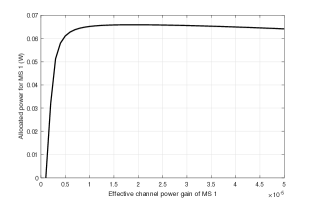
Refer to caption
Figure 4: Impact of effective power channel gain on allocated wireless power.

V-B Iteration Convergence Rate

The convergence of our proposed algorithm is assessed in Fig. 5, where the allowed error is set as ξ=105𝜉superscript105\xi=10^{-5}. Observe from Fig. 5(a) that the operator’s reward increases monotonically as the iteration evolves and tends to converge after only a few iterations (about 333 times for lossless compression and 777 for lossy compression). Next, let R(k)𝑅𝑘R(k) denote the operator’s reward after k𝑘k-th iteration and Rsuperscript𝑅R^{*} is the maximum operator’s reward of our proposed algorithm. Define Rgapsubscript𝑅gapR_{\rm{gap}} as the reward gap between R(k)𝑅𝑘R(k) and Rsuperscript𝑅R^{*} given as Rgap=|R(k)R|subscript𝑅gap𝑅𝑘superscript𝑅R_{\rm{gap}}=|R(k)-R^{*}|. Fig. 5(b) displays the curves of the reward gap verses the number of iterations. We can observe that the gap of our proposed algorithm almost linearly decreases as the iteration evolves, thus our proposed solution can be approximated as a first-order algorithm with linear local convergence rate [39].
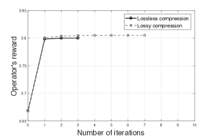
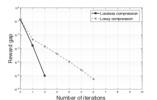
Refer to caption
(a) Operator’s reward vs. iteration
Refer to caption
(b) Reward gap vs. iteration
Figure 5: Convergence of our proposed algorithm.

V-C WPCS Performance

Three baseline policies are considered for our performance comparison. The first one is the baseline policy with fixed compression ratio (FCR) that jointly optimizes the power allocation, sensor transmission, and sensing-data size by following the approach in Section III-C. Specifically, the compression ratios for lossless and lossy compression are set as Rn=1.5subscript𝑅𝑛1.5R_{n}=1.5 and Rˇn=4subscriptˇ𝑅𝑛4\check{R}_{n}=4, respectively, which can achieve the maximum operator’s reward for the baseline policy with FCR. The second one is the baseline policy with equal power allocation (EPA), which jointly optimizes the sensor transmission, sensing-data size, and compression ratio given the power allocation policy. The third one is the baseline policy without compression, which can be regarded as a special case of the FCR with the compression ratio set as zero.
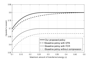
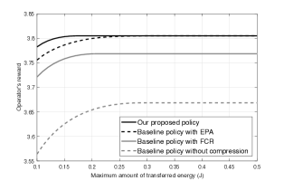
Refer to caption
(a) Lossless compression
Refer to caption
(b) Lossy compression
Figure 6: Operator’s reward vs. maximum amount of transferred energy.
Refer to caption
(a) Lossless compression
Refer to caption
(b) Lossy compression
Figure 7: Operator’s reward vs. time slot for crowd sensing.

The curves for the operator’s reward versus the maximum amount of transferred energy are displayed in Fig. 6 with the time duration for crowd sensing set as T=1𝑇1T=1 s. For lossless compression, it can be observed from Fig. 6(a) that the operator’s reward for our proposed policy is monotone-increasing with the growth of transferred energy in the small transferred-energy regime. However, when the amount of energy exceeds a threshold (of about 0.250.250.25 J), the performance cannot improve further by increasing the transferred energy. The reason is that the bottleneck in this case is no longer energy but other settings, such as the crowd-sensing duration.

Note that our proposed policy has significant performance gain over the policy with FCR and without compression, even when the maximum amount of transferred energy is sufficient. This shows the necessity of optimizing the compression ratios to improve system performance when the transferred energy is sufficient. In addition, among the three baseline policies, the one with EPA has the highest operator’s reward and approaches close-to-optimal performance in the large transferred energy regime. This is due to the fact that optimizing compression ratios can substantially reduce transmission energy consumption, thus allowing for using more energy to sense data for better data utility. For lossy compression, one can observe from Fig. 6(b) that our proposed policy yields higher operator’s reward with respect to the lossless counterpart for the case of small and large transferred energy, respectively. Other observations are similar to those in Fig. 6(a).

Fig. 7 demonstrates the curves of the operator’s reward versus the crowd-sensing duration for both compression methods. One can observe from Fig. 7(a) that for lossless compression, the operator’s reward is monotone-increasing with the extension of crowd-sensing duration, as it can reduce transmission-energy consumption so as to save more energy for data sensing. However, the growth rate of the operator’s reward slows down with the crowd-sensing duration. It indicates that extending a short crowd-sensing duration can substantially increase the operator’s reward. Moreover, in long crowd-sensing duration regime, lossy compression yields higher operator’s reward than in the lossless case. Other observations are similar to those in Fig. 6.
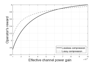
Refer to caption
Figure 8: Operator’s reward vs. effective channel power gain.

Finally, the impact of effective channel power gain on the compression method selection is evaluated in Fig. 8. Several observations are made as follows. First, the operator’s reward is observed to be a monotone-increasing function of the effective channel power gain. Next, lossy and lossless compression is preferred for relatively small and large effective channel power gains, respectively. The reason is that for poor channels, transmission-energy can dominate other components (e.g., sensing), and it can be substantially reduced by lossy compression due to efficient data-compression performance. However, when the channel is good enough, lossless compression can contribute to higher data utility with small compression energy, and thereby may be preferred over the lossy operation.

VI Concluding Remarks

This work proposed a multiuser WPCS system model and investigated a joint control of power allocation, sensing, compression, and transmission for maximizing the operator’s reward. It offered several insights into the control policies of the operator and the MSs. To be specific, for the operator, we showed that it should select the MSs for participating in the crowd sensing operation based on its configuration and the individual parameters of MSs. In addition, the optimal power allocation policy has a threshold-based structure depending on the derived crowd sensing priority function. For MSs, each selected sensor should control its compression ratio, sensor transmission, and sensing-data size for minimizing the resultant energy consumption. This work can be further extended to other interesting scenarios, such as cooperation among multiple operators and online control of multiuser WPCS systems.

-A Proof of Lemma 2

This lemma can be proved by contradiction. First, assume that {(n(s)),tn,Pn}superscriptsuperscriptsubscript𝑛𝑠superscriptsubscript𝑡𝑛superscriptsubscript𝑃𝑛\left\{\left(\ell_{n}^{(s)}\right)^{*},t_{n}^{*},P_{n}^{*}\right\} is the optimal solution satisfying αn(n(s))+tngnf((n(s))Rntn)<ηgnPnT0subscript𝛼𝑛superscriptsuperscriptsubscript𝑛𝑠superscriptsubscript𝑡𝑛subscript𝑔𝑛𝑓superscriptsuperscriptsubscript𝑛𝑠subscript𝑅𝑛superscriptsubscript𝑡𝑛𝜂subscript𝑔𝑛superscriptsubscript𝑃𝑛subscript𝑇0\alpha_{n}\left(\ell_{n}^{(s)}\right)^{*}\!+\!\frac{t_{n}^{*}}{g_{n}}f\left(\frac{\left(\ell_{n}^{(s)}\right)^{*}}{R_{n}t_{n}^{*}}\right)\!<\!\eta g_{n}P_{n}^{*}T_{0}. Then, there exists another feasible power allocation policy, denoted by Pn(1)superscriptsubscript𝑃𝑛1P_{n}^{(1)}, which satisfies Pn(1)<Pnsuperscriptsubscript𝑃𝑛1superscriptsubscript𝑃𝑛P_{n}^{(1)}<P_{n}^{*} and αn(n(s))+tngnf((n(s))Rntn)=ηgnPn(1)T0subscript𝛼𝑛superscriptsuperscriptsubscript𝑛𝑠superscriptsubscript𝑡𝑛subscript𝑔𝑛𝑓superscriptsuperscriptsubscript𝑛𝑠subscript𝑅𝑛superscriptsubscript𝑡𝑛𝜂subscript𝑔𝑛superscriptsubscript𝑃𝑛1subscript𝑇0\alpha_{n}{(\ell_{n}^{(s)})}^{*}\!+\!\frac{t_{n}^{*}}{g_{n}}f\left(\frac{\left(\ell_{n}^{(s)}\right)^{*}}{R_{n}t_{n}^{*}}\right)\!=\!\eta g_{n}P_{n}^{(1)}T_{0}. It leads to the following

n=1Nanlog(1+(n(s)))cn=1NPn(1)T0superscriptsubscript𝑛1𝑁subscript𝑎𝑛1superscriptsuperscriptsubscript𝑛𝑠𝑐superscriptsubscript𝑛1𝑁superscriptsubscript𝑃𝑛1subscript𝑇0\displaystyle\sum_{n=1}^{N}a_{n}\log(1+(\ell_{n}^{(s)})^{*})-c\sum_{n=1}^{N}P_{n}^{(1)}T_{0}
>n=1Nanlog(1+(n(s)))cn=1NPnT0,absentsuperscriptsubscript𝑛1𝑁subscript𝑎𝑛1superscriptsuperscriptsubscript𝑛𝑠𝑐superscriptsubscript𝑛1𝑁superscriptsubscript𝑃𝑛subscript𝑇0\displaystyle\qquad\qquad>\sum_{n=1}^{N}a_{n}\log(1+(\ell_{n}^{(s)})^{*})-c\sum_{n=1}^{N}P_{n}^{*}T_{0},

which contradicts the optimality. Similarly, if the optimal solution leads to βn(n(s))+tn<Tsubscript𝛽𝑛superscriptsuperscriptsubscript𝑛𝑠superscriptsubscript𝑡𝑛𝑇\beta_{n}\left(\ell_{n}^{(s)}\right)^{*}+t_{n}^{*}<T, then there exists another feasible policy with (n(s))(1)superscriptsuperscriptsubscript𝑛𝑠1(\ell_{n}^{(s)})^{(1)} that satisfies (n(s))(1)=Ttnβn>(n(s))superscriptsuperscriptsubscript𝑛𝑠1𝑇superscriptsubscript𝑡𝑛subscript𝛽𝑛superscriptsuperscriptsubscript𝑛𝑠(\ell_{n}^{(s)})^{(1)}=\frac{T-t_{n}^{*}}{\beta_{n}}>\left(\ell_{n}^{(s)}\right)^{*}. This new policy yields higher operator’s reward as

n=1Nanlog(1+(n(s))(1))cn=1NPnT0superscriptsubscript𝑛1𝑁subscript𝑎𝑛1superscriptsuperscriptsubscript𝑛𝑠1𝑐superscriptsubscript𝑛1𝑁superscriptsubscript𝑃𝑛subscript𝑇0\displaystyle\sum_{n=1}^{N}a_{n}\log(1+(\ell_{n}^{(s)})^{(1)})-c\sum_{n=1}^{N}P_{n}^{*}T_{0}
>n=1Nanlog(1+(n(s)))cn=1NPnT0,absentsuperscriptsubscript𝑛1𝑁subscript𝑎𝑛1superscriptsuperscriptsubscript𝑛𝑠𝑐superscriptsubscript𝑛1𝑁superscriptsubscript𝑃𝑛subscript𝑇0\displaystyle\qquad\qquad>\sum_{n=1}^{N}a_{n}\log(1+\left(\ell_{n}^{(s)}\right)^{*})-c\sum_{n=1}^{N}P_{n}^{*}T_{0},

thus contradicting the assumption. Combining the above together leads to the desired result.

-B Proof of Lemma 3

First, it is easy to see that n=1Nanlog(1+Ttnβn)superscriptsubscript𝑛1𝑁subscript𝑎𝑛1𝑇subscript𝑡𝑛subscript𝛽𝑛\sum_{n=1}^{N}a_{n}\log\left(1+\frac{T-t_{n}}{\beta_{n}}\right) is concave and αn(Ttn)ηgnβnsubscript𝛼𝑛𝑇subscript𝑡𝑛𝜂subscript𝑔𝑛subscript𝛽𝑛\frac{\alpha_{n}(T-t_{n})}{\eta g_{n}\beta_{n}} is linear for tnsubscript𝑡𝑛t_{n}. Then, the second derivative of tnηgn2f(TtnRnβntn)subscript𝑡𝑛𝜂superscriptsubscript𝑔𝑛2𝑓𝑇subscript𝑡𝑛subscript𝑅𝑛subscript𝛽𝑛subscript𝑡𝑛\frac{t_{n}}{\eta g_{n}^{2}}f\left(\frac{T-t_{n}}{{R_{n}}{\beta_{n}}{t_{n}}}\right) is N0(Tln2)2η(gnBRnβn)2tn32TtnBRnβntn>0subscript𝑁0superscript𝑇22𝜂superscriptsubscript𝑔𝑛𝐵subscript𝑅𝑛subscript𝛽𝑛2superscriptsubscript𝑡𝑛3superscript2𝑇subscript𝑡𝑛𝐵subscript𝑅𝑛subscript𝛽𝑛subscript𝑡𝑛0\frac{N_{0}{(T\ln 2)}^{2}}{\eta(g_{n}BR_{n}\beta_{n})^{2}t_{n}^{3}}2^{\frac{T-t_{n}}{BR_{n}\beta_{n}t_{n}}}>0 for 0<tn<T0subscript𝑡𝑛𝑇0<{t_{n}}<T; thus, it is a convex function. It follows that the objective function, being a summation over a set of convex functions, preserves the convexity. Combining it with the convex constraints yields the desired result.

-C Proof of Corollary 1

From (1), the utility weight can be expressed as:

ansubscript𝑎𝑛\displaystyle a_{n} =[(Tln2BRnβntn1)eTln2BRnβntnln2BRnβn+αngnN0βn+1]absentdelimited-[]𝑇2𝐵subscript𝑅𝑛subscript𝛽𝑛superscriptsubscript𝑡𝑛1superscript𝑒𝑇2𝐵subscript𝑅𝑛subscript𝛽𝑛superscriptsubscript𝑡𝑛2𝐵subscript𝑅𝑛subscript𝛽𝑛subscript𝛼𝑛subscript𝑔𝑛subscript𝑁0subscript𝛽𝑛1\displaystyle=\left[\left(\frac{T\ln 2}{BR_{n}\beta_{n}t_{n}^{*}}-1\right)e^{\frac{T\ln 2}{BR_{n}\beta_{n}t_{n}^{*}}-\frac{\ln 2}{BR_{n}\beta_{n}}}+\frac{\alpha_{n}g_{n}}{N_{0}\beta_{n}}+1\right]
×(λ+c)N0[βn+(Ttn)]ηgn2.absentsuperscript𝜆𝑐subscript𝑁0delimited-[]subscript𝛽𝑛𝑇superscriptsubscript𝑡𝑛𝜂superscriptsubscript𝑔𝑛2\displaystyle\qquad\qquad\times\frac{(\lambda^{*}+c)N_{0}[\beta_{n}+(T-t_{n}^{*})]}{\eta g_{n}^{2}}.

Given a1<a2subscript𝑎1subscript𝑎2a_{1}<a_{2}, it can be directly observed from the above equation that t1>t2subscript𝑡1subscript𝑡2t_{1}>t_{2}. As for the effective channel power gain, it should satisfy the following equation:

gn[anηgn(λ+c)N0[βn+(Ttn)]αnN0βn]subscript𝑔𝑛delimited-[]subscript𝑎𝑛𝜂subscript𝑔𝑛superscript𝜆𝑐subscript𝑁0delimited-[]subscript𝛽𝑛𝑇superscriptsubscript𝑡𝑛subscript𝛼𝑛subscript𝑁0subscript𝛽𝑛\displaystyle g_{n}\left[\frac{a_{n}\eta g_{n}}{(\lambda^{*}+c)N_{0}[\beta_{n}+(T-t_{n}^{*})]}-\frac{\alpha_{n}}{N_{0}\beta_{n}}\right]
=(Tln2BRnβntn1)eTln2BRnβntnln2BRnβn+1.absent𝑇2𝐵subscript𝑅𝑛subscript𝛽𝑛superscriptsubscript𝑡𝑛1superscript𝑒𝑇2𝐵subscript𝑅𝑛subscript𝛽𝑛superscriptsubscript𝑡𝑛2𝐵subscript𝑅𝑛subscript𝛽𝑛1\displaystyle\qquad\qquad=\left(\frac{T\ln 2}{BR_{n}\beta_{n}t_{n}^{*}}-1\right)e^{\frac{T\ln 2}{BR_{n}\beta_{n}t_{n}^{*}}-\frac{\ln 2}{BR_{n}\beta_{n}}}+1. (28)

Note that both the right hand-side of (-C) and N0[βn+(Ttn)]subscript𝑁0delimited-[]subscript𝛽𝑛𝑇superscriptsubscript𝑡𝑛N_{0}[\beta_{n}+(T-t_{n}^{*})] are decreasing with tnsubscript𝑡𝑛t_{n}. It means that if g1<g2subscript𝑔1subscript𝑔2g_{1}<g_{2}, it should be satisfied that t1t2subscript𝑡1subscript𝑡2t_{1}\geq t_{2}, thus completing the proof.

-D Proof of Proposition 2

First, combing αn(n(s))+tngnf((n(s))Rntn)=ηgnPnT0subscript𝛼𝑛superscriptsuperscriptsubscript𝑛𝑠superscriptsubscript𝑡𝑛subscript𝑔𝑛𝑓superscriptsuperscriptsubscript𝑛𝑠subscript𝑅𝑛superscriptsubscript𝑡𝑛𝜂subscript𝑔𝑛superscriptsubscript𝑃𝑛subscript𝑇0\alpha_{n}\left(\ell_{n}^{(s)}\right)^{*}+\frac{t_{n}^{*}}{g_{n}}f\left(\frac{\left(\ell_{n}^{(s)}\right)^{*}}{R_{n}t_{n}^{*}}\right)=\eta g_{n}P_{n}^{*}T_{0} and βn(n(s))+tn=Tsubscript𝛽𝑛superscriptsuperscriptsubscript𝑛𝑠superscriptsubscript𝑡𝑛𝑇\beta_{n}\left(\ell_{n}^{(s)}\right)^{*}+t_{n}^{*}=T gives

Pn=1ηgnT0[tngnf(TtnRnβntn)+αn(Ttn)βn].superscriptsubscript𝑃𝑛1𝜂subscript𝑔𝑛subscript𝑇0delimited-[]superscriptsubscript𝑡𝑛subscript𝑔𝑛𝑓𝑇superscriptsubscript𝑡𝑛subscript𝑅𝑛subscript𝛽𝑛superscriptsubscript𝑡𝑛subscript𝛼𝑛𝑇superscriptsubscript𝑡𝑛subscript𝛽𝑛P_{n}^{*}=\frac{1}{\eta g_{n}T_{0}}\left[\frac{t_{n}^{*}}{g_{n}}f\left(\frac{T-t_{n}^{*}}{R_{n}\beta_{n}t_{n}^{*}}\right)+\frac{\alpha_{n}(T-t_{n}^{*})}{\beta_{n}}\right].

Next, the first and the second derivative of Pnsubscript𝑃𝑛P_{n} are calculated as follows.

Pntn=N0ηgn2T0[(1Tln2BRnβntn)2TtnBRnβntn1]αnηβngnT0,subscript𝑃𝑛subscript𝑡𝑛subscript𝑁0𝜂superscriptsubscript𝑔𝑛2subscript𝑇0delimited-[]1𝑇2𝐵subscript𝑅𝑛subscript𝛽𝑛subscript𝑡𝑛superscript2𝑇subscript𝑡𝑛𝐵subscript𝑅𝑛subscript𝛽𝑛subscript𝑡𝑛1subscript𝛼𝑛𝜂subscript𝛽𝑛subscript𝑔𝑛subscript𝑇0\displaystyle\frac{\partial P_{n}}{\partial t_{n}}\!=\!\frac{N_{0}}{\eta g_{n}^{2}T_{0}}\left[\left(1-\frac{T\ln 2}{BR_{n}\beta_{n}t_{n}}\right)2^{\frac{T-t_{n}}{BR_{n}\beta_{n}t_{n}}}\!-\!1\right]\!-\!\frac{\alpha_{n}}{\eta\beta_{n}g_{n}T_{0}},
2Pntn2=N0(Tln2)2ηT0(gnBRnβn)2tn32TtnBRnβntn.superscript2subscript𝑃𝑛superscriptsubscript𝑡𝑛2subscript𝑁0superscript𝑇22𝜂subscript𝑇0superscriptsubscript𝑔𝑛𝐵subscript𝑅𝑛subscript𝛽𝑛2superscriptsubscript𝑡𝑛3superscript2𝑇subscript𝑡𝑛𝐵subscript𝑅𝑛subscript𝛽𝑛subscript𝑡𝑛\displaystyle\frac{\partial^{2}P_{n}}{\partial t_{n}^{2}}\!=\!\frac{N_{0}{(T\ln 2)}^{2}}{\eta T_{0}(g_{n}BR_{n}\beta_{n})^{2}t_{n}^{3}}2^{\frac{T-t_{n}}{BR_{n}\beta_{n}t_{n}}}.

It can be observed that 2Pntn2>0superscript2subscript𝑃𝑛superscriptsubscript𝑡𝑛20\frac{\partial^{2}P_{n}}{\partial t_{n}^{2}}>0 for 0tnT0subscript𝑡𝑛𝑇0\leq t_{n}\leq T. Hence, Pntnsubscript𝑃𝑛subscript𝑡𝑛\frac{\partial P_{n}}{\partial t_{n}} is monotone-increasing for 0tnT0subscript𝑡𝑛𝑇0\leq t_{n}\leq T and

(Pntn)max=Pntn|tn=T=Nnln2ηgn2BRnβnT0αnηβngnT0<0.subscriptsubscript𝑃𝑛subscript𝑡𝑛maxevaluated-atsubscript𝑃𝑛subscript𝑡𝑛subscript𝑡𝑛𝑇subscript𝑁𝑛2𝜂superscriptsubscript𝑔𝑛2𝐵subscript𝑅𝑛subscript𝛽𝑛subscript𝑇0subscript𝛼𝑛𝜂subscript𝛽𝑛subscript𝑔𝑛subscript𝑇00\left(\frac{\partial P_{n}}{\partial t_{n}}\right)_{\rm{max}}\!=\!\frac{\partial P_{n}}{\partial t_{n}}\bigg{|}_{t_{n}=T}\!=\!-\frac{N_{n}\ln 2}{\eta g_{n}^{2}BR_{n}\beta_{n}T_{0}}\!-\!\frac{\alpha_{n}}{\eta\beta_{n}g_{n}T_{0}}\!<\!0.

It means that Pnsubscript𝑃𝑛P_{n} is monotone decreasing with tnsubscript𝑡𝑛t_{n} and (Pn)min=Pn|tn=T=0subscriptsubscript𝑃𝑛minevaluated-atsubscript𝑃𝑛subscript𝑡𝑛𝑇0({P_{n}})_{\rm{min}}={P_{n}}|_{t_{n}=T}=0. Combining (12a) and 0tnT0subscript𝑡𝑛𝑇0\leq t_{n}\leq T yields

λsuperscript𝜆\displaystyle\lambda^{*} >anηgnβn+(Ttn)αnβnN0gn[(1Tln2BRnβntn)2TtnBRnβntn1]cabsentsubscript𝑎𝑛𝜂subscript𝑔𝑛subscript𝛽𝑛𝑇superscriptsubscript𝑡𝑛subscript𝛼𝑛subscript𝛽𝑛subscript𝑁0subscript𝑔𝑛delimited-[]1𝑇2𝐵subscript𝑅𝑛subscript𝛽𝑛superscriptsubscript𝑡𝑛superscript2𝑇superscriptsubscript𝑡𝑛𝐵subscript𝑅𝑛subscript𝛽𝑛superscriptsubscript𝑡𝑛1𝑐\displaystyle>\frac{\frac{a_{n}\eta g_{n}}{\beta_{n}+(T-t_{n}^{*})}}{\frac{\alpha_{n}}{\beta_{n}}-\frac{N_{0}}{g_{n}}\left[\left(1-\frac{T\ln 2}{BR_{n}\beta_{n}t_{n}^{*}}\right)2^{\frac{T-t_{n}^{*}}{BR_{n}\beta_{n}t_{n}^{*}}}-1\right]}-c
=anηgnqn(r)+qn(s)+qn(c)eϵRn+N0ln2gnBRnc=φn.absentsubscript𝑎𝑛𝜂subscript𝑔𝑛superscriptsubscript𝑞𝑛𝑟superscriptsubscript𝑞𝑛𝑠superscriptsubscript𝑞𝑛𝑐superscript𝑒italic-ϵsubscript𝑅𝑛subscript𝑁02subscript𝑔𝑛𝐵subscript𝑅𝑛𝑐subscript𝜑𝑛\displaystyle=\frac{a_{n}\eta g_{n}}{q_{n}^{(r)}+q_{n}^{(s)}+q_{n}^{(c)}e^{\epsilon R_{n}}+\frac{N_{0}\ln 2}{g_{n}BR_{n}}}-c=\varphi_{n}.

If λ<φnsuperscript𝜆subscript𝜑𝑛\lambda^{*}<\varphi_{n}, the optimal sensing time will violate the time constraint tn>Tsuperscriptsubscript𝑡𝑛𝑇t_{n}^{*}\!>\!T; thus, the sensor will not be selected and no power will be allocated to it i.e., Pn=0subscript𝑃𝑛0P_{n}=0, which completes the proof.

-E Proof of Lemma 5

Based on (20a), for Rn=1superscriptsubscript𝑅𝑛1R_{n}^{*}=1, it can be established that N0ln2gnB2n(s)tnB(qn(c)+λ^fn)ϵeϵ<0.subscript𝑁02subscript𝑔𝑛𝐵superscript2superscriptsubscript𝑛𝑠superscriptsubscript𝑡𝑛𝐵superscriptsubscript𝑞𝑛𝑐superscript^𝜆subscript𝑓𝑛italic-ϵsuperscript𝑒italic-ϵ0\frac{N_{0}\ln 2}{g_{n}B}2^{\frac{\ell_{n}^{(s)}}{t_{n}^{*}B}}-\left(q_{n}^{(c)}+\frac{\widehat{\lambda}^{*}}{f_{n}}\right){\epsilon}e^{\epsilon}<0. Combining it with the optimal conditions, tn=Tn(s)snsuperscriptsubscript𝑡𝑛𝑇superscriptsubscript𝑛𝑠subscript𝑠𝑛t_{n}^{*}=T-\frac{\ell_{n}^{(s)}}{s_{n}} and λ^=N0gn[(n(s)ln2tnB1)2n(s)tnB+1]superscript^𝜆subscript𝑁0subscript𝑔𝑛delimited-[]superscriptsubscript𝑛𝑠2superscriptsubscript𝑡𝑛𝐵1superscript2superscriptsubscript𝑛𝑠superscriptsubscript𝑡𝑛𝐵1\widehat{\lambda}^{*}=\frac{N_{0}}{g_{n}}\left[\left(\frac{\ell_{n}^{(s)}\ln 2}{t_{n}^{*}B}-1\right)2^{\frac{\ell_{n}^{(s)}}{t_{n}^{*}B}}+1\right], leads to the desired result.

-F Proof of Proposition 4

Based on (20c), at least one of the two equations λ^=0superscript^𝜆0\widehat{\lambda}^{*}=0 or tn+n(s)(eϵRneϵ)fn+n(s)snT=0superscriptsubscript𝑡𝑛superscriptsubscript𝑛𝑠superscript𝑒italic-ϵsuperscriptsubscript𝑅𝑛superscript𝑒italic-ϵsubscript𝑓𝑛superscriptsubscript𝑛𝑠subscript𝑠𝑛𝑇0t_{n}^{*}+\frac{\ell_{n}^{(s)}\left(e^{\epsilon R_{n}^{*}}-e^{\epsilon}\right)}{f_{n}}+\frac{\ell_{n}^{(s)}}{s_{n}}-T=0 should be satisfied. Assume that tn+n(s)(eϵRneϵ)fn+n(s)snT0superscriptsubscript𝑡𝑛superscriptsubscript𝑛𝑠superscript𝑒italic-ϵsuperscriptsubscript𝑅𝑛superscript𝑒italic-ϵsubscript𝑓𝑛superscriptsubscript𝑛𝑠subscript𝑠𝑛𝑇0t_{n}^{*}+\frac{\ell_{n}^{(s)}\left(e^{\epsilon R_{n}^{*}}-e^{\epsilon}\right)}{f_{n}}+\frac{\ell_{n}^{(s)}}{s_{n}}-T\neq 0, then it has λ^=0superscript^𝜆0\widehat{\lambda}^{*}=0, which leads to Rnsuperscriptsubscript𝑅𝑛R_{n}^{*}\to\infty according to (20b). This, however, contradicts the finite compression ratio. Hence, it should satisfy: tn+n(s)(eϵRneϵ)fn+n(s)sn=Tsuperscriptsubscript𝑡𝑛superscriptsubscript𝑛𝑠superscript𝑒italic-ϵsuperscriptsubscript𝑅𝑛superscript𝑒italic-ϵsubscript𝑓𝑛superscriptsubscript𝑛𝑠subscript𝑠𝑛𝑇t_{n}^{*}+\frac{\ell_{n}^{(s)}\left(e^{\epsilon R_{n}^{*}}-e^{\epsilon}\right)}{f_{n}}+\frac{\ell_{n}^{(s)}}{s_{n}}=T. The optimal solution should satisfy (20a) as

(qn(c)+λ^fn)ϵeϵRn1gn(Rn)2f(n(s)tnRn)=0.superscriptsubscript𝑞𝑛𝑐superscript^𝜆subscript𝑓𝑛italic-ϵsuperscript𝑒italic-ϵsuperscriptsubscript𝑅𝑛1subscript𝑔𝑛superscriptsuperscriptsubscript𝑅𝑛2superscript𝑓superscriptsubscript𝑛𝑠superscriptsubscript𝑡𝑛superscriptsubscript𝑅𝑛0\left(q_{n}^{(c)}+\frac{\widehat{\lambda}^{*}}{f_{n}}\right)\epsilon e^{\epsilon R_{n}^{*}}-\frac{1}{g_{n}(R_{n}^{*})^{2}}f^{\prime}\left(\frac{\ell_{n}^{(s)}}{t_{n}^{*}R_{n}^{*}}\right)=0.

Combining the above with the optimal conditions, λ^=1gng(n(s)tnRn)superscript^𝜆1subscript𝑔𝑛𝑔superscriptsubscript𝑛𝑠superscriptsubscript𝑡𝑛superscriptsubscript𝑅𝑛\widehat{\lambda}^{*}=-\frac{1}{g_{n}}g\left(\frac{\ell_{n}^{(s)}}{t_{n}^{*}R_{n}^{*}}\right) and tn=Tn(s)(eϵRneϵ)fnn(s)snsuperscriptsubscript𝑡𝑛𝑇superscriptsubscript𝑛𝑠superscript𝑒italic-ϵsuperscriptsubscript𝑅𝑛superscript𝑒italic-ϵsubscript𝑓𝑛superscriptsubscript𝑛𝑠subscript𝑠𝑛t_{n}^{*}=T-\frac{\ell_{n}^{(s)}\left(e^{\epsilon R_{n}^{*}}-e^{\epsilon}\right)}{f_{n}}-\frac{\ell_{n}^{(s)}}{s_{n}} according to (20b) and (20c), produces the desired result.

-G Proof of Lemma 6

The first derivative of function z(Rn)𝑧subscript𝑅𝑛z({R_{n}}) is

z(Rn)Rn𝑧subscript𝑅𝑛subscript𝑅𝑛\displaystyle\frac{\partial z(R_{n})}{\partial R_{n}} =N0ln2BRn2gn[2Rn+ln2[Rnd(Rn)]B[Rnd(Rn)]2(1Rnd(Rn)d(Rn))]absentsubscript𝑁02𝐵superscriptsubscript𝑅𝑛2subscript𝑔𝑛delimited-[]2subscript𝑅𝑛2superscriptdelimited-[]subscript𝑅𝑛𝑑subscript𝑅𝑛𝐵superscriptdelimited-[]subscript𝑅𝑛𝑑subscript𝑅𝑛21subscript𝑅𝑛superscript𝑑subscript𝑅𝑛𝑑subscript𝑅𝑛\displaystyle\!=\!\frac{N_{0}\ln 2}{BR_{n}^{2}g_{n}}\left[\frac{2}{R_{n}}+\frac{\ln 2[R_{n}d(R_{n})]^{\prime}}{B[R_{n}d(R_{n})]^{2}}\left(1\!-\!\frac{R_{n}d^{\prime}({R_{n}})}{d(R_{n})}\right)\right]
×eln2BRnd(Rn)+[qn(c)1gnfng(1d(Rn)Rn)]ϵ2eϵRn.absentsuperscript𝑒2𝐵subscript𝑅𝑛𝑑subscript𝑅𝑛delimited-[]superscriptsubscript𝑞𝑛𝑐1subscript𝑔𝑛subscript𝑓𝑛𝑔1𝑑subscript𝑅𝑛subscript𝑅𝑛superscriptitalic-ϵ2superscript𝑒italic-ϵsubscript𝑅𝑛\displaystyle\leavevmode\nobreak\ \leavevmode\nobreak\ \leavevmode\nobreak\ \times\!e^{\frac{\ln 2}{BR_{n}d(R_{n})}}\!+\!\left[q_{n}^{(c)}\!-\!\frac{1}{g_{n}f_{n}}g\left(\frac{1}{d(R_{n})R_{n}}\right)\right]\epsilon^{2}e^{\epsilon R_{n}}\!.

First, it has [Rnd(Rn)]=d(Rn)Rnd(Rn)superscriptdelimited-[]subscript𝑅𝑛𝑑subscript𝑅𝑛𝑑subscript𝑅𝑛subscript𝑅𝑛superscript𝑑subscript𝑅𝑛[R_{n}d({R_{n}})]^{{}^{\prime}}\!=\!d({R_{n}})\!-\!R_{n}d^{\prime}({R_{n}}). Hence, [Rnd(Rn)]>0superscriptdelimited-[]subscript𝑅𝑛𝑑subscript𝑅𝑛0[R_{n}d({R_{n}})]^{\prime}>0 when d(Rn)>Rnd(Rn)𝑑subscript𝑅𝑛subscript𝑅𝑛superscript𝑑subscript𝑅𝑛d({R_{n}})>R_{n}d^{\prime}({R_{n}}) and [Rnd(Rn)]<0superscriptdelimited-[]subscript𝑅𝑛𝑑subscript𝑅𝑛0[R_{n}d({R_{n}})]^{\prime}<0 when d(Rn)<Rnd(Rn)𝑑subscript𝑅𝑛subscript𝑅𝑛superscript𝑑subscript𝑅𝑛d({R_{n}})<R_{n}d^{\prime}({R_{n}}). Combining these together leads to:

ln2[Rnd(Rn)]B[Rnd(Rn)]2(1Rnd(Rn)d(Rn))>0,forRn[1,Rmax].formulae-sequence2superscriptdelimited-[]subscript𝑅𝑛𝑑subscript𝑅𝑛𝐵superscriptdelimited-[]subscript𝑅𝑛𝑑subscript𝑅𝑛21subscript𝑅𝑛superscript𝑑subscript𝑅𝑛𝑑subscript𝑅𝑛0forsubscript𝑅𝑛1subscript𝑅max\frac{\ln 2[R_{n}d(R_{n})]^{\prime}}{B[R_{n}d(R_{n})]^{2}}\left(1-\frac{R_{n}d^{\prime}({R_{n}})}{d(R_{n})}\right)>0,\leavevmode\nobreak\ \leavevmode\nobreak\ \text{for}\leavevmode\nobreak\ R_{n}\in[1,R_{\rm{max}}].

Further, the first derivative of function g(x)𝑔𝑥g(x) is

g(x)=xf′′(x)=N0ln22B22xB<0,forx>0.formulae-sequencesuperscript𝑔𝑥𝑥superscript𝑓′′𝑥subscript𝑁0superscript22superscript𝐵2superscript2𝑥𝐵0for𝑥0g^{\prime}(x)=-xf^{\prime\prime}(x)=-\frac{N_{0}\ln 2^{2}}{B^{2}}2^{\frac{x}{B}}<0,\leavevmode\nobreak\ \leavevmode\nobreak\ \text{for}\leavevmode\nobreak\ x>0.

It means that g(x)𝑔𝑥g(x) is monotone-decreasing with x𝑥x and thus g(x)g(x)|x=0=0𝑔𝑥evaluated-at𝑔𝑥𝑥00g(x)\leq g(x)|_{x=0}=0 for x>0𝑥0x>0. Since 1d(Rn)Rn>01𝑑subscript𝑅𝑛subscript𝑅𝑛0\frac{1}{d(R_{n})R_{n}}>0, it has [qn(c)1gnfng(1d(Rn)Rn)]>0delimited-[]superscriptsubscript𝑞𝑛𝑐1subscript𝑔𝑛subscript𝑓𝑛𝑔1𝑑subscript𝑅𝑛subscript𝑅𝑛0\left[q_{n}^{(c)}-\frac{1}{g_{n}f_{n}}g\left(\frac{1}{d(R_{n})R_{n}}\right)\right]>0 for x>0𝑥0x>0. Combining the above considerations leads to z(Rn)Rn>0𝑧subscript𝑅𝑛subscript𝑅𝑛0\frac{\partial z(R_{n})}{\partial R_{n}}>0 for Rn[1,Rmax]subscript𝑅𝑛1subscript𝑅maxR_{n}\in[1,R_{\rm{max}}], thus completing the proof.

-H Proof of Corollary 5

Define a function φ(Rn)𝜑subscript𝑅𝑛\varphi(R_{n}) as φ(Rn)=qn(c)gn𝜑subscript𝑅𝑛superscriptsubscript𝑞𝑛𝑐subscript𝑔𝑛\varphi(R_{n})=q_{n}^{(c)}g_{n}. According to (2)), it has

φ(Rn)=1fng(1d(Rn)Rn)+1Rn2ϵeϵRnf(1d(Rn)Rn).𝜑subscript𝑅𝑛1subscript𝑓𝑛𝑔1𝑑subscript𝑅𝑛subscript𝑅𝑛1superscriptsubscript𝑅𝑛2italic-ϵsuperscript𝑒italic-ϵsubscript𝑅𝑛superscript𝑓1𝑑subscript𝑅𝑛subscript𝑅𝑛\varphi(R_{n})=\frac{1}{f_{n}}g\left(\frac{1}{d(R_{n})R_{n}}\right)+\frac{1}{R_{n}^{2}\epsilon e^{\epsilon R_{n}}}f^{\prime}\left(\frac{1}{d(R_{n})R_{n}}\right).

The derivation of φ(Rn)𝜑subscript𝑅𝑛\varphi(R_{n}) is

φ(Rn)Rn𝜑subscript𝑅𝑛subscript𝑅𝑛\displaystyle\frac{\partial\varphi(R_{n})}{\partial R_{n}} =[2+ϵRnϵeϵRn+ln2[Rnd(Rn)]B[Rnd(Rn)]2(1RnϵeϵRnfnd(Rn))]absentdelimited-[]2italic-ϵsubscript𝑅𝑛italic-ϵsuperscript𝑒italic-ϵsubscript𝑅𝑛2superscriptdelimited-[]subscript𝑅𝑛𝑑subscript𝑅𝑛𝐵superscriptdelimited-[]subscript𝑅𝑛𝑑subscript𝑅𝑛21subscript𝑅𝑛italic-ϵsuperscript𝑒italic-ϵsubscript𝑅𝑛subscript𝑓𝑛𝑑subscript𝑅𝑛\displaystyle=-\left[\frac{2+\epsilon}{R_{n}\epsilon e^{\epsilon R_{n}}}+\frac{\ln 2[R_{n}d(R_{n})]^{\prime}}{B[R_{n}d(R_{n})]^{2}}\left(1-\frac{R_{n}\epsilon e^{\epsilon R_{n}}}{f_{n}d(R_{n})}\right)\right]
×N0ln2BRn2ϵeϵRneln2BRnd(Rn).absentsubscript𝑁02𝐵superscriptsubscript𝑅𝑛2italic-ϵsuperscript𝑒italic-ϵsubscript𝑅𝑛superscript𝑒2𝐵subscript𝑅𝑛𝑑subscript𝑅𝑛\displaystyle\quad\quad\quad\times\frac{N_{0}\ln 2}{BR_{n}^{2}\epsilon e^{\epsilon R_{n}}}e^{\frac{\ln 2}{BR_{n}d(R_{n})}}.

Since ln2[Rnd(Rn)]B[Rnd(Rn)]2(1RnϵeϵRnfnd(Rn))2superscriptdelimited-[]subscript𝑅𝑛𝑑subscript𝑅𝑛𝐵superscriptdelimited-[]subscript𝑅𝑛𝑑subscript𝑅𝑛21subscript𝑅𝑛italic-ϵsuperscript𝑒italic-ϵsubscript𝑅𝑛subscript𝑓𝑛𝑑subscript𝑅𝑛\frac{\ln 2[R_{n}d(R_{n})]^{\prime}}{B[R_{n}d(R_{n})]^{2}}\left(1-\frac{R_{n}\epsilon e^{\epsilon R_{n}}}{f_{n}d(R_{n})}\right) is always positive as proved in Appendix -G, the function φ(Rn)𝜑subscript𝑅𝑛\varphi(R_{n}) is monotone-decreasing for Rn[1,Rmax]subscript𝑅𝑛1subscript𝑅maxR_{n}\!\in\![1,R_{\rm{max}}]. Given q1(c)>q2(c)superscriptsubscript𝑞1𝑐superscriptsubscript𝑞2𝑐q_{1}^{(c)}\!>\!q_{2}^{(c)}, it can be derived that R1<R2subscript𝑅1subscript𝑅2R_{1}\!<\!R_{2}. Using a similar approach, it can be proved that R1<R2subscript𝑅1subscript𝑅2R_{1}\!<\!R_{2} when g1>g2subscript𝑔1subscript𝑔2g_{1}\!>\!g_{2}, thus completing the proof.

-I Proof of Lemma 7

The first derivative of zˇ(rn)ˇ𝑧subscript𝑟𝑛\check{z}({r_{n}}) is

N0ln2Bgnrn2[2rn+ln2[rndˇ(rn)]B[rndˇ(rn)]2(1rndˇ(rn)dˇ(rn))]eln2Brndˇ(rn)+limit-fromsubscript𝑁02𝐵subscript𝑔𝑛superscriptsubscript𝑟𝑛2delimited-[]2subscript𝑟𝑛2superscriptdelimited-[]subscript𝑟𝑛ˇ𝑑subscript𝑟𝑛𝐵superscriptdelimited-[]subscript𝑟𝑛ˇ𝑑subscript𝑟𝑛21subscript𝑟𝑛superscriptˇ𝑑subscript𝑟𝑛ˇ𝑑subscript𝑟𝑛superscript𝑒2𝐵subscript𝑟𝑛ˇ𝑑subscript𝑟𝑛\displaystyle\frac{N_{0}\ln 2}{Bg_{n}r_{n}^{2}}\left[\frac{2}{r_{n}}+\frac{\ln 2[r_{n}\check{d}(r_{n})]^{\prime}}{B[r_{n}\check{d}(r_{n})]^{2}}\left(1-\frac{r_{n}\check{d}^{\prime}({r_{n}})}{\check{d}(r_{n})}\right)\right]e^{\frac{\ln 2}{Br_{n}\check{d}(r_{n})}}+
(6+4ϵrn2)rnqn(c)ϵeϵrn2g(1dˇ(rn)rn)(6+4ϵrn2)ϵrngnfneϵrn2.64italic-ϵsuperscriptsubscript𝑟𝑛2subscript𝑟𝑛superscriptsubscript𝑞𝑛𝑐italic-ϵsuperscript𝑒italic-ϵsuperscriptsubscript𝑟𝑛2𝑔1ˇ𝑑subscript𝑟𝑛subscript𝑟𝑛64italic-ϵsuperscriptsubscript𝑟𝑛2italic-ϵsubscript𝑟𝑛subscript𝑔𝑛subscript𝑓𝑛superscript𝑒italic-ϵsuperscriptsubscript𝑟𝑛2\displaystyle\quad(6+4\epsilon r_{n}^{2})r_{n}q_{n}^{(c)}\epsilon e^{\epsilon r_{n}^{2}}-g\left(\frac{1}{\check{d}(r_{n})r_{n}}\right)\frac{(6+4\epsilon r_{n}^{2})\epsilon r_{n}}{g_{n}f_{n}}e^{\epsilon r_{n}^{2}}.

The derivative of function rndˇ(rn)subscript𝑟𝑛ˇ𝑑subscript𝑟𝑛r_{n}\check{d}({r_{n}}) is dˇ(rn)rndˇ(rn)ˇ𝑑subscript𝑟𝑛subscript𝑟𝑛superscriptˇ𝑑subscript𝑟𝑛\check{d}({r_{n}})-r_{n}\check{d}^{\prime}({r_{n}}). Since [rndˇ(rn)]>0superscriptdelimited-[]subscript𝑟𝑛ˇ𝑑subscript𝑟𝑛0[r_{n}\check{d}({r_{n}})]^{\prime}>0 when dˇ(rn)>rndˇ(rn)ˇ𝑑subscript𝑟𝑛subscript𝑟𝑛superscriptˇ𝑑subscript𝑟𝑛\check{d}({r_{n}})>r_{n}\check{d}^{\prime}({r_{n}}) and [rndˇ(rn)]<0superscriptdelimited-[]subscript𝑟𝑛ˇ𝑑subscript𝑟𝑛0[r_{n}\check{d}({r_{n}})]^{\prime}<0 when dˇ(rn)<rndˇ(rn)ˇ𝑑subscript𝑟𝑛subscript𝑟𝑛superscriptˇ𝑑subscript𝑟𝑛\check{d}({r_{n}})<r_{n}\check{d}^{\prime}({r_{n}}), the item ln2[rndˇ(rn)]B[rndˇ(rn)]2(1rndˇ(rn)dˇ(rn))2superscriptdelimited-[]subscript𝑟𝑛ˇ𝑑subscript𝑟𝑛𝐵superscriptdelimited-[]subscript𝑟𝑛ˇ𝑑subscript𝑟𝑛21subscript𝑟𝑛superscriptˇ𝑑subscript𝑟𝑛ˇ𝑑subscript𝑟𝑛\frac{\ln 2[r_{n}\check{d}(r_{n})]^{\prime}}{B[r_{n}\check{d}(r_{n})]^{2}}\left(1-\frac{r_{n}\check{d}^{\prime}({r_{n}})}{\check{d}(r_{n})}\right) is always positive. Moreover, g(x)<0𝑔𝑥0g(x)<0 when x>0𝑥0x>0 according to Appendix -G. Since 1dˇ(rn)rn>01ˇ𝑑subscript𝑟𝑛subscript𝑟𝑛0\frac{1}{\check{d}(r_{n})r_{n}}>0, the item [(6+4ϵrn2)rnqn(c)ϵeϵrn2g(1dˇ(rn)rn)(6+4ϵrn2)ϵrngnfneϵrn2]delimited-[]64italic-ϵsuperscriptsubscript𝑟𝑛2subscript𝑟𝑛superscriptsubscript𝑞𝑛𝑐italic-ϵsuperscript𝑒italic-ϵsuperscriptsubscript𝑟𝑛2𝑔1ˇ𝑑subscript𝑟𝑛subscript𝑟𝑛64italic-ϵsuperscriptsubscript𝑟𝑛2italic-ϵsubscript𝑟𝑛subscript𝑔𝑛subscript𝑓𝑛superscript𝑒italic-ϵsuperscriptsubscript𝑟𝑛2\left[(6+4\epsilon r_{n}^{2})r_{n}q_{n}^{(c)}\epsilon e^{\epsilon r_{n}^{2}}-g\left(\frac{1}{\check{d}(r_{n})r_{n}}\right)\frac{(6+4\epsilon r_{n}^{2})\epsilon r_{n}}{g_{n}f_{n}}e^{\epsilon r_{n}^{2}}\right] is always positive. Hence, Zˇ(rn)rn>0ˇ𝑍subscript𝑟𝑛subscript𝑟𝑛0\frac{\partial\check{Z}(r_{n})}{\partial r_{n}}>0 for rn[1,rmax]subscript𝑟𝑛1subscript𝑟maxr_{n}\in[1,r_{\rm{max}}], thus completing the proof.

References

  • [1] I. F. Akyildiz, W. Su, Y. Sankarasubramaniam, and E. Cayirci, “Wireless sensor networks: A survey,” Comput. netw., vol. 38, no. 4, pp. 393–422, 2002.
  • [2] R. K. Ganti, F. Ye, and H. Lei, “Mobile crowdsensing: Current state and future challenges,” IEEE Commun. Mag., vol. 49, no. 11, pp. 32–39, 2011.
  • [3] O. Galinina, K. Mikhaylov, K. Huang, S. Andreev, and Y. Koucheryavy, “Wirelessly powered urban crowd sensing over wearables: Trading energy for data,” [Online]. Available: https://arxiv.org/pdf/1611.05910.pdf.
  • [4] H. Ma, D. Zhao, and P. Yuan, “Opportunities in mobile crowd sensing,” IEEE Commun. Mag., vol. 52, no. 8, pp. 29–35, 2014.
  • [5] V. Petrov, A. Samuylov, V. Begishev, D. Moltchanov, S. Andreev, K. Samouylov, and Y. Koucheryavy, “Vehicle-based relay assistance for opportunistic crowdsensing over narrowband IoT (NB-IoT),” IEEE Internet Things J., vol. PP, no. 99, pp. 1–1, 2017.
  • [6] X. Zhang, Z. Yang, W. Sun, Y. Liu, S. Tang, K. Xing, and X. Mao, “Incentives for mobile crowd sensing: A survey,” IEEE Commun. Surveys Tuts., vol. 18, no. 1, pp. 54–67, 2016.
  • [7] Z. Feng, Y. Zhu, Q. Zhang, L. M. Ni, and A. V. Vasilakos, “TRAC: Truthful auction for location-aware collaborative sensing in mobile crowdsourcing,” in Proc. IEEE Infocom, 2014, pp. 1231–1239.
  • [8] L. Duan, T. Kubo, K. Sugiyama, J. Huang, T. Hasegawa, and J. Walrand, “Incentive mechanisms for smartphone collaboration in data acquisition and distributed computing,” in Proc. IEEE Infocom, 2012, pp. 1701–1709.
  • [9] S. Yang, F. Wu, S. Tang, X. Gao, B. Yang, and G. Chen, “On designing data quality-aware truth estimation and surplus sharing method for mobile crowdsensing,” IEEE J. Sel. Areas Commun., vol. 35, no. 4, pp. 832–847, 2017.
  • [10] M. A. Alsheikh, D. Niyato, D. Leong, P. Wang, and Z. Han, “Privacy management and optimal pricing in people-centric sensing,” IEEE J. Sel. Areas Commun., vol. 35, no. 4, pp. 906–920, 2017.
  • [11] X. Lu, P. Wang, D. Niyato, D. I. Kim, and Z. Han, “Wireless networks with RF energy harvesting: A contemporary survey,” IEEE Commun. Surveys Tuts., vol. 17, no. 2, pp. 757–789, 2015.
  • [12] Y. Zeng, B. Clerckx, and R. Zhang, “Communications and signals design for wireless power transmission,” IEEE Trans. Commun., vol. 65, no. 5, pp. 2264–2290, 2016.
  • [13] A. Ghazanfari, H. Tabassum, and E. Hossain, “Ambient RF energy harvesting in ultra-dense small cell networks: Performance and trade-offs,” IEEE Wireless Commun., vol. 23, no. 2, pp. 38–45, 2016.
  • [14] R. Zhang and C. K. Ho, “MIMO broadcasting for simultaneous wireless information and power transfer,” IEEE Trans. Wireless Commun., vol. 12, no. 5, pp. 1989–2001, 2013.
  • [15] J. Park and B. Clerckx, “Joint wireless information and energy transfer in a two-user MIMO interference channel,” IEEE Trans. Wireless Commun., vol. 12, no. 8, pp. 4210–4221, 2013.
  • [16] P. Popovski, A. M. Fouladgar, and O. Simeone, “Interactive joint transfer of energy and information,” IEEE Trans. Commun., vol. 61, no. 5, pp. 2086–2097, 2013.
  • [17] Z. Ding, S. M. Perlaza, I. Esnaola, and H. V. Poor, “Power allocation strategies in energy harvesting wireless cooperative networks,” IEEE Trans. Wireless Commun., vol. 13, no. 2, pp. 846–860, 2014.
  • [18] Z. Ding, I. Krikidis, B. Sharif, and H. V. Poor, “Wireless information and power transfer in cooperative networks with spatially random relays,” IEEE Trans. Wireless Commun., vol. 13, no. 8, pp. 4440–4453, 2014.
  • [19] Z. Zheng, L. Song, D. Niyato, and Z. Han, “Resource allocation in wireless powered relay networks: A bargaining game approach,” IEEE Trans. Vehi. Techn., vol. 66, no. 7, pp. 6310–6323, 2017.
  • [20] D. W. K. Ng, E. S. Lo, and R. Schober, “Wireless information and power transfer: Energy efficiency optimization in OFDMA systems,” IEEE Trans. Wireless Commun., vol. 12, no. 12, pp. 6352–6370, 2013.
  • [21] S. Lee, R. Zhang, and K. Huang, “Opportunistic wireless energy harvesting in cognitive radio networks,” IEEE Trans. Wireless Commun., vol. 12, no. 9, pp. 4788–4799, 2013.
  • [22] D. W. K. Ng, E. S. Lo, and R. Schober, “Multiobjective resource allocation for secure communication in cognitive radio networks with wireless information and power transfer,” IEEE Trans. Veh. Technol., vol. 65, no. 5, pp. 3166–3184, 2016.
  • [23] C.-F. Liu, M. Maso, S. Lakshminarayana, C.-H. Lee, and T. Q. Quek, “Simultaneous wireless information and power transfer under different CSI acquisition schemes,” IEEE Trans. Wireless Commun., vol. 14, no. 4, pp. 1911–1926, 2015.
  • [24] M. Gregori and M. Payaró, “Energy-efficient transmission for wireless energy harvesting nodes,” IEEE Trans. Wireless Commun., vol. 12, no. 3, pp. 1244–1254, 2013.
  • [25] Y. Zeng, R. Zhang, and T. J. Lim, “Throughput maximization for UAV-enabled mobile relaying systems,” IEEE Trans. Commun., vol. 64, no. 12, pp. 4983–4996, 2016.
  • [26] C. You, K. Huang, and H. Chae, “Energy efficient mobile cloud computing powered by wireless energy transfer,” IEEE J. Sel. Areas Commun., vol. 34, no. 5, pp. 1757–1771, 2016.
  • [27] L. Xie, Y. Shi, Y. T. Hou, and A. Lou, “Wireless power transfer and applications to sensor networks,” IEEE Wireless Commun., vol. 20, no. 4, pp. 140–145, 2013.
  • [28] K. W. Choi, L. Ginting, P. A. Rosyady, A. A. Aziz, and D. I. Kim, “Wireless-powered sensor networks: How to realize,” IEEE Trans. Wireless Commun., vol. 16, no. 1, pp. 221–234, 2017.
  • [29] J. Xu, Z. Zhong, and B. Ai, “Wireless powered sensor networks: Collaborative energy beamforming considering sensing and circuit power consumption,” IEEE Commun. Lett., vol. 5, no. 4, pp. 344–347, 2016.
  • [30] S. Guo, F. Wang, Y. Yang, and B. Xiao, “Energy-efficient cooperative transmission for simultaneous wireless information and power transfer in clustered wireless sensor networks,” IEEE Trans. Commun., vol. 63, no. 11, pp. 4405–4417, 2015.
  • [31] K. Han and K. Huang, “Wirelessly powered backscatter communication networks: modeling, coverage, and capacity,” IEEE Trans. Wireless Commun., vol. 16, no. 4, pp. 2548–2561, 2017.
  • [32] M. Bhardwaj, T. Garnett, and A. P. Chandrakasan, “Upper bounds on the lifetime of sensor networks,” in Proc. IEEE ICC, 2001, pp. 785–790.
  • [33] A. V. D. Ven, “Linux OS data compression options: Comparing behavior,” https://clearlinux.org/blogs/linux-os-data-compression-options-comparing-behavior, 2017.
  • [34] A. P. Chandrakasan, S. Sheng, and R. W. Brodersen, “Low-power CMOS digital design,” IEEE J. Solid-State Circuits, vol. 27, no. 4, pp. 473–484, 1992.
  • [35] C. J. V. den Branden Lambrecht and O. Verscheure, “Perceptual quality measure using a spatiotemporal model of the human visual system,” in Proc. SPIE, vol. 2668, 1996, pp. 450–461.
  • [36] D. Yang, G. Xue, X. Fang, and J. Tang, “Crowdsourcing to smartphones: Incentive mechanism design for mobile phone sensing,” in Proc. MobiCom, 2012, pp. 173–184.
  • [37] S. Boyd and L. Vandenberghe, Convex Optimization.   Cambridge University Press, 2004.
  • [38] A. Thiagarajan, L. Ravindranath, H. Balakrishnan, S. Madden, and L. Girod, “Accurate, low-energy trajectory mapping for mobile devices,” in Proc. NSDI, 2011, pp. 267–280.
  • [39] M. Schatzman, Numerical analysis: A mathematical introduction.   Oxford University Press, 2002.