Two-phase Thermodynamic Model for Computing Entropies of Liquids Reanalyzed

Abstract

The two-phase thermodynamic (2PT) model [J. Chem. Phys., 119, 11792 (2003)] provides a promising paradigm to efficiently determine the ionic entropies of liquids from molecular dynamics (MD). In this model, the vibrational density of states (VDoS) of a liquid is decomposed into a diffusive gas-like component and a vibrational solid-like component. By treating the diffusive component as hard sphere (HS) gas and the vibrational component as harmonic oscillators, the ionic entropy of the liquid is determined. Here we examine three issues crucial for practical implementations of the 2PT model: (i) the mismatch between the VDoS of the liquid system and that of the HS gas; (ii) the excess entropy of the HS gas; (iii) the partition of the gas-like and solid-like components. Some of these issues have not been addressed before, yet they profoundly change the entropy predicted from the model. Based on these findings, a revised 2PT formalism is proposed and successfully tested in systems with Lennard-Jones potentials as well as many-atom potentials of liquid metals. Aside from being capable of performing quick entropy estimations for a wide range of systems, the formalism also supports fine-tuning to accurately determine entropies at specific thermal states.

I introduction

Entropy $(S)$ is a fundamental while somewhat peculiar thermodynamic quantity in molecular dynamics (MD) simulations.Allen and Tildesley (1989); Frenkel and Smit (2002) It is one of the basic inputs, along with energy $(E)$, pressure $(P)$, density ($\rho$), and temperature $(T)$, to determine the system’s free energy essential for establishing phase diagrams and other thermodynamic properties. However, unlike $E$, $P$, $\rho$, and $T$, entropy can not be defined as time averages over phase space trajectories,Allen and Tildesley (1989); Frenkel and Smit (2002) and special techniques are needed to evaluate entropy in MD. For solids, entropy can be evaluated through the power spectrum (vibrational density of states, VDoS) of the velocity autocorrelation function (VACF) using phonon gas model (PGM).Wallace (1972); Grimvall (1999); Fultz (2010); Sun et al. (2010); Zhang et al. (2014) PGM takes into account lattice anharmonicity via temperature-dependent phonon frequencies and is applicable even to strongly anharmonic crystals.Sun et al. (2014); Lu et al. (2017) However, PGM is not suitable for liquids as diffusion of atoms, a characteristic feature of fluids, cannot be described by phonons. To overcome this difficulty, Lin et al.Lin et al. (2003) proposed an ingenious two-phase thermodynamic (2PT) model. In this model, the VDoS of a liquid is decomposed into a diffusive gas-like component and a vibrational solid-like component. Entropy associated with the diffusive component is determined from the hard spheres (HS) model, that with the vibrational component is from the harmonic oscillator (phonon) model. The 2PT model requires only one post-processing of the MD trajectory to evaluate entropy. Thus it is much more efficient than the conventional thermodynamic integration (TI) approach which involves many separate MD simulations along the integration path. Because of this, the 2PT model has attracted considerable attention and has been applied to many systems including Ar,Lin et al. (2003) CO₂,Huang et al. (2011) H₂O,Lin et al. (2010) liquid metals,Desjarlais (2013); Robert et al. (2015); Jakse and Pasturel (2016) silicates and oxides,Boates and Bonev (2013) etc.

In essence, the 2PT model relies on phonons to describe vibration and HS to describe diffusion. The former is a natural extension of the well-established PGM for solids and can be regarded as reliable. The latter, as it turns out, is more problematic and requires careful consideration. Here we focus on three issues that are related to HS. The first issue, as noticed by Desjarlais,Desjarlais (2013) is that the VDoS of HS gas declines more slowly with frequency than that of the actual liquid. As a result, the VDoS of the gas-like component is larger than the total VDoS at high frequencies. This mismatch in VDoS was found to cause significant overestimation of entropy (up to 0.3 to 0.4 $k_{B}$ per atom) in ab initio MD (AIMD) simulations of liquid metals.Desjarlais (2013) The second issue, which has not been addressed so far, is the explicit formula used to evaluate the excess entropy ($S_{{\rm ex}}$) of HS gas. The excess entropy is defined as the entropy difference between non-ideal and ideal gases under the same physical condition. Here the same physical condition refers to either identical $T$ and $\rho$, or identical $T$ and $P$. In the original 2PT paper,Lin et al. (2003) Lin et al. applied the Carnahan-Starling formulaCarnahan and Starling (1970) to compute $S_{{\rm ex}}$ under identical $T$ and $\rho$. However, a closer inspection would reveal that the Carnahan-Starling formula actually corresponds to $S_{{\rm ex}}$ under identical $T$ and $P$.Carnahan and Starling (1970); O’Connell and Haile (2005); Hansen and McDonald (2006) The two formulas, $S_{{\rm ex}}(T,\>\rho)$ and $S_{{\rm ex}}(T,\>P)$, differ by a term $\ln(z)$, where $z$ is the compressibility of the HS gas.O’Connell and Haile (2005) As will be shown in the paper, removing this $\ln(z)$ term causes profound changes to the predicted entropies. It is surprising that the predicability of a model hinges on an apparently misplaced formula. Resolving this puzzle leads to the third issue we would address: the partition of the gas-like and solid-like components. Indeed, entropy predicted by the 2PT model relies on the gas-solid partition and this partition can be refined to improve the accuracy of the model.

In this paper, we introduce a revised 2PT formalism which resolves the above three issues. The formalism is first validated with liquid Ar using Lennard-Jones potential, in the same fashion as Lin et al.’s original work. It is then applied to liquid metals using Sutton-Chen many-atom potentials.Sutton and Chen (1990) The adoption of classical potentials, rather than AIMD, allows us to perform extensive TI calculations to check the accuracy of the entropies from the 2PT model. The analytic nature of Sutton-Chen potentials is also ideal for demonstrating how the softness of interatomic potentials affects the predicted 2PT entropies. We stress that while only classical potentials are considered in the present paper, the proposed formalism should also be applicable to AIMD simulations as the underlying physics is identical.

II original 2pt formalism

The starting point of a 2PT calculationLin et al. (2003) is the VACF $C(t)$ and its power spectrum (VDoS) $F(\nu)$, evaluated in MD as

$$C(t) =\frac{1}{3(N-1)}\sum_{i=1}^{N}m\left\langle\mathbf{v}_{i}\left(0\right)\cdot\mathbf{v}_{i}\left(t\right)\right\rangle,$$ (1)

$$F(\nu) =\frac{12}{k_{B}T}\int_{0}^{\infty}C(t)\cos(2\pi\nu t)dt.$$ (2)

Here $m$ is the mass of an atom, $N$ is the total number of atoms, ${\rm{\bf v}}_{i}\left(t\right)$ denotes the velocity of the ith atom at time $t$, and $\left\langle\cdots\right\rangle$ stands for ensemble average, $k_{B}$ is the Boltzmann’s constant. With such definitions, we have (i) $C(0)=k_{B}T$; (ii) $\int_{0}^{\infty}F(\nu)d\nu=3$; (iii) the VDoS at zero frequency $F\left(0\right)$ is proportional to the diffusion coefficient $D$ asHansen and McDonald (2006); McQuarrie (2000)

$$F\left(0\right) =\frac{12m}{k_{B}T}D.$$ (3)

A non-zero $F(0)$ indicates that the system is in fluid state.

Next, $C(t)$ and $F\left(\nu\right)$ are partitioned into a gas-like component and a solid-like component as

$$C(t) =f_{g}C_{g}(t)+(1-f_{g})C_{s}(t),$$ (4)

$$F\left(\nu\right) =f_{g}F_{g}\left(\nu\right)+\left(1-f_{g}\right)F_{s}\left(\nu\right),$$ (5)

where the subscripts distinguish the gas-like($g$) and solid-like($s$) subsystems, respectively, $f_{g}$ denotes the gas-like fraction of the system and takes value between $0$ (completely solid) and $1$ (completely gas). According to the Enskog theory of HS model, $C_{g}(t)$ equals $k_{B}T\exp(-\alpha t)$,McQuarrie (2000); Hansen and McDonald (2006) where $\alpha$ is a parameter to be calculated, and

$$F_{g}(\nu) =\frac{12\alpha}{\alpha^{2}+4\pi^{2}\nu^{2}}.$$ (6)

Note $F_{g}(\nu)$ obeys the sum rule $\int_{0}^{\infty}F_{g}(\nu)d\nu=3$, an useful feature in subsequent entropy evaluations. Since the diffusive VDoS at zero frequency $F(0)$ should be completely attributed to the gas component, we have

$$F(0) =f_{g}F_{g}(0)=\frac{12f_{g}}{\alpha}.$$ (7)

Thus $\alpha$, and subsequently $F_{g}(\nu)$ , can be determined once $f_{g}$ is known. The VDoS associated with the solid-like component $(1-f_{g})F_{s}(\nu)$ can then be determined as $F(\nu)-f_{g}F_{g}(\nu)$.

To evaluate $f_{g}$, Lin et al made two further assumptions:Lin et al. (2003) (i) $f_{g}=\frac{D}{D_{0}}$, where $D_{0}$ is the HS diffusivity in the low density limit (the Chapman-Enskog result); (ii) the diffusivity of the gas component can be determined analytically using the Enskog theory for dense HS, and it is $1/f_{g}$ times larger than the diffusivity of the whole system. With these two assumptions, $f_{g}$, as well as the packing fraction of HS, are uniquely determined and the partition of gas-solid components is accomplished (see Appendix A for a general derivation) .

The partition of gas-solid components can be interpreted as the liquid system under study is dynamically equivalent to a combination of two subsystems: one is HS gas with $f_{g}N$ particles, the other is harmonic oscillators with VDoS equaling $N(1-f_{g})F_{s}(\nu)$. Entropy of the liquid equals the sum of the entropies of subsystems. For the solid subsystem, the associated entropy $S_{s}$ is determined as

$$S_{s} =Nk_{{}_{B}}\left(1-f_{g}\right)\int_{0}^{\infty}F_{s}\left(\nu\right)W_{s}\left(\nu\right)d\nu,$$ (8)

where

$$W_{s}\left(\nu\right) =\frac{h\nu/k_{B}T}{e^{h\nu/k_{B}T}-1}-\ln\left[1-e^{-h\nu/k_{B}T}\right]$$

$$\approx 1-\ln(h\nu/k_{B}T)\>\>\>\>\>\>\>\>(h\nu\ll k_{B}T)$$ (9)

corresponds to the entropy of a quantum (classical) harmonic oscillatorBerens et al. (1983) and $h$ represents the Planck’s constant. Entropy associated with the gas subsystem $S_{g}$ is determined as

$$S_{g} =Nk_{B}f_{g}\int_{0}^{\infty}F_{g}(\nu)W_{g}d\nu,$$ (10)

where the weighting function $W_{g}$ is the sum of the ideal gas (IG) contribution $W_{{\rm IG}}$ and excess (${\rm ex}$) contribution $W_{{\rm ex}}$,Carnahan and Starling (1970) i.e. $W_{g}=W_{{\rm IG}}+W_{{\rm ex}}$. For a given $T$ and $\rho$ (here $\rho=f_{g}N/V$), $W_{{\rm IG}}$ is expressed as

$$W_{{\rm IG}} =\frac{1}{3k_{B}}S_{{\rm IG}}(T,\>\rho)$$

$$=\frac{1}{3}\left\{\frac{5}{2}+\ln\left[\left(\frac{2\pi mk_{B}T}{h^{2}}\right)^{3/2}\frac{V}{f_{g}N}\right]\right\}$$ (11)

and the corresponding $W_{{\rm ex}}$ should beO’Connell and Haile (2005); Hansen and McDonald (2006)

$$W_{{\rm ex}} =\frac{1}{3k_{B}}S_{{\rm ex}}(T,\>\rho)$$

$$=\frac{1}{3}\frac{\gamma\left(3\gamma-4\right)}{\left(1-\gamma\right)^{2}},$$ (12)

where $S_{{\rm IG}}(T,\,\rho)$ is the entropy per atom of the ideal gas, $S_{{\rm ex}}$ is the excess entropy per atom of the HS gas, $\gamma$ ($\gamma\equiv\frac{\pi\rho}{6}\sigma^{3}$, $\sigma$ is the hard sphere diameter) is the packing fraction. However in the original 2PT paper, a different weighting function was used,Carnahan and Starling (1970)

$$W_{{\rm ex}}^{\prime} =\frac{1}{3}\left\{\frac{\gamma\left(3\gamma-4\right)}{\left(1-\gamma\right)^{2}}+\ln z\right\},$$ (13)

which in fact corresponds to the excess entropy under identical $T$ and $P$ (see Appendix B for a derivation). In the following session we show how this extra $\ln z$ term in $W_{{\rm ex}}$ affects the predicted entropies.

Eqs. (8) and (10) contain integrals with infinity as upper bounds. In practice, this infinite upper bound is replaced by a finite $\nu_{0}$, which should be sufficiently large to ensure the numerical integration result converges to the exact value. This is particularly important for $S_{g}$, where $F_{g}(\nu)$ decreases slowly as $\nu^{-2}$ and $W_{g}$ is $\nu$-independent. An alternative way to evaluate $S_{g}$ is to apply the sum rule $\int_{0}^{\infty}F_{g}(\nu)d\nu=3$, which leads to $S_{g}=3Nk_{B}f_{g}W_{g}$.

III liquid argon

Liquid argon is the prototype of simple fluids. Its phase diagram and thermodynamic properties have been determined accurately over a wide $T$ and $\rho$ range.Johnson et al. (1993) This makes liquid argon an ideal model system for methodological developments. The inter-atomic potential of liquid argon takes the form

$$V(r) =4\epsilon\left[\left(\frac{\sigma}{r}\right)^{12}-\left(\frac{\sigma}{r}\right)^{6}\right],$$

where $\sigma=3.405$ Å, $\epsilon/k_{B}=119.8$ K, $m=39.948$ g/mol. For generality, $T$ and $\rho$ are measured in reduced units as $T^{\star}=k_{B}T/\epsilon$, $\rho^{\star}=\rho\sigma^{3}$. In the original 2PT paper,Lin et al. (2003) Five $\rho^{\star}$ ($1.10$, $0.85$, $0.70$, $0.40$, and $0.05$) and four $T^{\star}$ ($1.8$, $1.4$, $1.1$, and $0.9$) were considered. These $(\rho^{\star},\>T^{\star})$ cover fluid, solid, metastable and unstable states. Here we focus on $(\rho^{\star},\>T^{\star})$ conditions where argon is in the fluid state, the intended target of the 2PT model. Moreover, the sampling of $T^{\star}$ is increased to elucidate the trends in $S(T)$. MD simulationsTodorov et al. (2006) were performed with the same setup as Lin et al.,Lin et al. (2003) i.e., the system contained 512 atoms, the time step was 8 fs, each simulation first ran $10\>000$ steps for equilibration, then another $20\>000$ to $50\>000$ steps for production. Moreover, the maximum entropy methodPress et al. (1986) was applied to minimize the statistical noises and produce smooth VDoS.

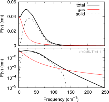
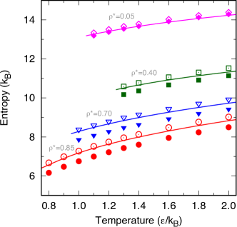
Figure 1: (a) Partitions of the VDoS of liquid argon at $\rho^{\star}=0.85$, $T^{\star}=1.1$ in the original 2PT model. (b) Entropies at various $\rho^{\star}$ and $T^{\star}$. Open symbols denote results obtained with the same $S_{{\rm ex}}$ formula as Lin et al.,Lin et al. (2003) closed symbols denote results with the right formula (without $\ln z$), solid lines represent the MBWR EOS.Johnson et al. (1993)

Fig. 1(a) shows a representative $F(\nu)$ at $\rho^{\star}=0.85$, $T^{\star}=1.1$ and the partition of gas-like and solid-like components. We see that the gas-like component $f_{g}F_{g}(\nu)$ takes the maximum at $\nu=0$ where $f_{g}F_{g}(0)=F(0)$, then declines monotonically as $\nu$ increases. In contrast, the solid-like component $(1-f_{g})F_{s}(\nu)$ is zero at $\nu=0$ but makes predominant contribution to $F(\nu)$ at higher frequencies. A subtle feature, manifest only in the logarithmic scale, is that $f_{g}F_{g}(\nu)$ becomes larger than the total $F(\nu)$ when $\nu\apprge 140$ cm^-1. This mismatch between $f_{g}F_{g}(\nu)$ and $F(\nu)$ was first noticed by Desjarlais in his AIMD simulations of liquid metals.Desjarlais (2013) Here we see it is also present in liquid argon. To quantify this mismatch, we define an auxiliary function $F_{a}(\nu)$ as

$$F_{a}(\nu) =\begin{cases}f_{g}F_{g}(\nu)-F(\nu),&f_{g}F_{g}(\nu)>F(\nu)\\ 0,&f_{g}F_{g}(\nu)\leq F(\nu)\end{cases}.$$

Although $F_{a}(\nu)$ seems negligibly small, it spans a very wide frequency range (diminishes as $\nu^{-2}$ at high $\nu$) and the overall contribution is still notable. At $\rho^{\star}=0.85$, $T^{\star}=1.1$, the integral $\int_{0}^{\infty}F_{a}(\nu)\>d\nu=0.0625$, or $2\%$ of the total VDoS. Here the integration was performed numerically by replacing the infinite upper bound with a large $\nu_{0}$ (2084.6 cm^-1), and the residue $\int_{\nu_{0}}^{\infty}F_{a}(\nu)d\nu$ is less than $5\times 10^{-4}$. If we discard the entropy associated with $F_{a}(\nu)$, either by enforcing the VDoS of the gas-component equals $F(\nu)$ when $f_{g}F_{g}(\nu)>F(\nu)$, or by adopting a smaller $\nu_{0}$ (e. g. 200 cm^-1) when evaluating the entropy integrals in Eqs. (8) and (10), we are able to reproduce Lin et al.’s results,Lin et al. (2003) shown as open symbols in Fig. 1(b) and tabulated in Table 1. These results agree with the modified Benedict-Webb-Rubin (MBWR) EOSJohnson et al. (1993) fairly well, however one should be aware that this agreement is achieved when (i) the entropy associated with $F_{{\rm a}}(\nu)$ is ignored, (ii) the excess entropy of HS was evaluated using Eq. (13), instead of Eq. (12). If the right formula for weighting function (without $\ln(z)$) was applied, entropy will drop significantly (solid symbols in Fig. 1(b)). For instance, at $\rho^{\star}=0.85$ , $T^{\star}=1.1$, the original 2PT prediction is $7.51$ $k_{B}$ per atom, about $1$% higher than the MBWR result ($7.42$ $k_{B}$). After dropping the $\ln(z)$ term in $W_{g}$, the 2PT prediction becomes 6.99 $k_{B}$ per atom, nearly $6\%$ lower than the MBWR result. Only at low densities ( e. g. $\rho^{\star}=0.05$) where the system is close to ideal gas and $S_{{\rm ex}}$ is small, the effect of the $\ln(z)$ term is inconsequential.

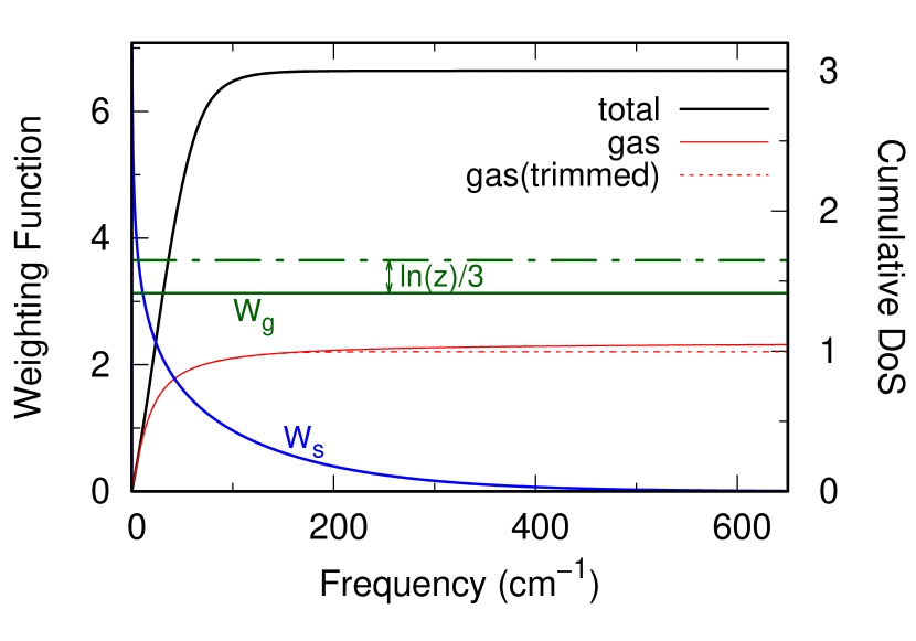
Figure 2: Weighting functions (left axis) $W_{s}(\nu)$, $W_{g}$ and cumulative VDoS (right axis) : $I(\nu)=\int_{0}^{\nu}F(\nu)d\nu$ (“total”), $I_{g}(\nu)=\int_{0}^{v}f_{g}F_{g}(\nu)d\nu$ (“gas”), and $I_{g,t}(\nu)=\int_{0}^{\nu}[f_{g}F_{g}(\nu)-F_{a}(\nu)]d\nu$ (“gas(trimmed)”) for liquid argon at $\rho^{\star}=0.85$, $T^{\star}=1.1$.

To better appreciate these results, we present in Fig. 2 the weighting functions $W_{s}(\nu)$, $W_{g}$ (with and without $\ln(z)$), and cumulative VDoS: $I(\nu)=\int_{0}^{\nu}F(\nu)d\nu$ (“total”), $I_{g}(\nu)=\int_{0}^{v}f_{g}F_{g}(\nu)d\nu$ (“gas”), and $I_{g,t}(\nu)=\int_{0}^{\nu}[f_{g}F_{g}(\nu)-F_{a}(\nu)]d\nu$ (“gas(trimmed)”) at $\rho^{\star}=0.85$ , $T^{\star}=1.1$. The last integral $I_{g,t}(\nu)$ corresponds to the case where the high-frequency tail of $f_{g}F_{g}(\nu)$ is trimmed by enforcing the VDoS of the gas component equals $F(\nu)$ when $f_{g}F_{g}(\nu)>F(\nu)$. At this $\rho^{\star}$ and $T^{\star}$, $f_{g}=0.35$, $\gamma=0.33$ , and $\ln(z)/3=0.52$ . In comparison, $W_{{\rm ex}}$ and $W_{{\rm IG}}$ equal $-0.75$ and $3.88$, respectively. Therefore with or without the $\ln(z)$ term in $W_{g}$ makes a big difference in the predicted 2PT entropy. Also, we note that $I(\nu)$ and $I_{g,t}(\nu)$ saturate with $\nu$ quickly ($\sim 200$ cm^-1) , while $I_{g}(\nu)$ saturates much slowly due to the presence of $F_{a}(\nu)$. If we include $F_{a}(\nu)$ in the VDoS of the gas component, $S_{g}$ will increase by $\int_{0}^{\infty}F_{a}(\nu)W_{g}d\nu=0.20$ $k_{B}$ per atom; if we treat $F_{a}(\nu)$ as harmonic oscillators (solid-component), the corresponding entropy is $\int_{0}^{\infty}F_{a}(\nu)W_{s}(\nu)d\nu=0.01$ $k_{B}$ per atom. The difference between these two cases is because in regions where $F_{a}(\nu)$ is non-zero, $W_{s}(\nu)\ll W_{g}$. These information will be useful when we try to revise the 2PT model.

IV revised 2PT model

Table 1: Entropies (in $k_{B}$ per atom) of Lennard-Jones fluid at selected $\rho^{\star}$ and $T^{\star}$. “MBWR EOS” denotes data from Ref. Johnson et al., 1993, “2PT” and “2PT (w/o $\ln z$)” correspond to results from the original 2PT formalism with and without the $\ln(z)$ term in $W_{g}$, “R2PT ($\delta$)” represents results from the revised 2PT model with the value of $\delta$ in the parentheses. Uncertainties in the 2PT calculations are estimated to be $0.02$ $k_{B}$ per atom.

$\rho^{\star}$	$T^{\star}$	MBWR EOS	2PT	2PT (w/o $\ln z$)	R2PT ($1.0$)	R2PT ($1.5$)
	0.8	6.57	6.67	6.16	6.33	6.50
	1.1	7.42	7.51	6.99	7.18	7.36
0.85	1.4	7.99	8.13	7.60	7.79	7.98
	1.8	8.58	8.76	8.23	8.43	8.62
	2.0	8.83	9.02	8.49	8.70	8.88
	1.0	8.28	8.38	7.86	8.04	8.21
0.70	1.4	8.99	9.15	8.63	8.83	8.99
	1.8	9.51	9.70	9.20	9.40	9.55
	1.3	10.51	10.58	10.17	10.33	10.39
0.40	1.6	10.92	11.06	10.67	10.83	10.88
	1.8	11.14	11.31	10.91	11.08	11.13
	1.1	13.27	13.34	13.18	13.24	13.19
0.05	1.4	13.67	13.79	13.67	13.72	13.67
	1.8	14.07	14.23	14.11	14.17	14.12

In the prior section we demonstrate a dilemma in the original 2PT formalism: the spurious $\ln(z)$ term in evaluating $S_{{\rm ex}}$ should be dropped, but removing this term spoils the good agreement and entropy becomes significantly underestimated. A question arises naturally: is it possible to modify the 2PT formalism, such that it adopts the right formula for $S_{{\rm ex}}$ and yet gives accurate entropy? In the following we construct a revised 2PT model that meets this requirement.

We have shown that $f_{g}F_{g}(\nu)$ is larger than $F(\nu)$ at high frequencies and the excess VDoS is defined as $F_{a}(\nu)$. Since entropies associated with $F_{a}(\nu)$ were not accounted for in the original calculation, our first revision of the model is to include such contributions. This is more sensible than simply discarding $F_{a}(\nu)$ if one considers the fundamental difference between diffusion and vibration: For vibrations, it is okay to consider entropy contributions from various frequency components of VDoS individually, as they represent different harmonic oscillators whose motions are independent. Diffusion is a far more complex type of motion with all frequency components coupled to each other and only $f_{g}F_{g}(\nu)$ as a whole is physically meaningful. To determine entropy associated with $f_{g}F_{g}(\nu)$, we replace the numerical integration $S_{g}=Nk_{B}f_{g}\int_{0}^{\nu_{0}}F_{g}(\nu)W_{g}d\nu,$ where $\nu_{0}$ is the upper bound of the VDoS, with the closed form $3Nk_{B}f_{g}W_{g}$. This allows us to avoid the truncation error that may arise from a finite $\nu_{0}$. A consequence of including $F_{a}(\nu)$ in the VDoS of the gas component is that the corresponding VDoS of the solid component becomes negative, as $(1-f_{g})F_{s}(\nu)\equiv F(\nu)-f_{g}F_{g}(\nu)=-F_{a}(\nu)$. The appearance of negative solid VDoS can be interpreted as follows: Imagine the liquid system under study is attached with an assemblage of auxiliary harmonic oscillators with VDoS $F_{a}(\nu)$. The VDoS of the combined system is $F(\nu)+F_{a}(\nu)$. To get entropy associated with $F(\nu)$, one may first perform standard 2PT calculation on the combined system, then subtract the entropies of auxiliary harmonic oscillators. Thus the negative solid VDoS is just book-keeping of auxiliary harmonic oscillators, with entropy $S_{s,a}=-Nk_{B}\int_{0}^{\infty}F_{a}(\nu)W_{s}(\nu)d\nu$. Note at high $T$, $f_{g}F_{g}(\nu)$ may slightly exceed $F(\nu)$ also near $\nu=0$ (see supplementary material). Such mismatch is readily handled via $F_{a}(\nu)$, just like the mismatch in the high $\nu$ region. In contrast to $S_{g}$, $S_{s,a}$ is easy to converge in numerical integration as $W_{s}(\nu)$ decreases exponentially at high $\nu$. The value of $S_{s,a}$ is small. At $\rho^{\star}=0.85$, $T^{\star}=1.1$, $S_{s,a}$ is just $-0.01$ $k_{B}$ per atom, whereas the increase in $S_{g}$ after accounting for $F_{a}(\nu)$ is $0.20$ $k_{B}$ per atom. Thus the overall effect of including $F_{a}(\nu)$ is to increase entropy by $0.19$ $k_{B}$ per atom. This moves the 2PT predictions (tabulated with label “R2PT(1.0)” in Table 1) closer to the standard MBWR results, but the remaining differences ($3\%$) is still substantial compared to the desired accuracy ($1\%$) in practical applications.Fultz (2010)

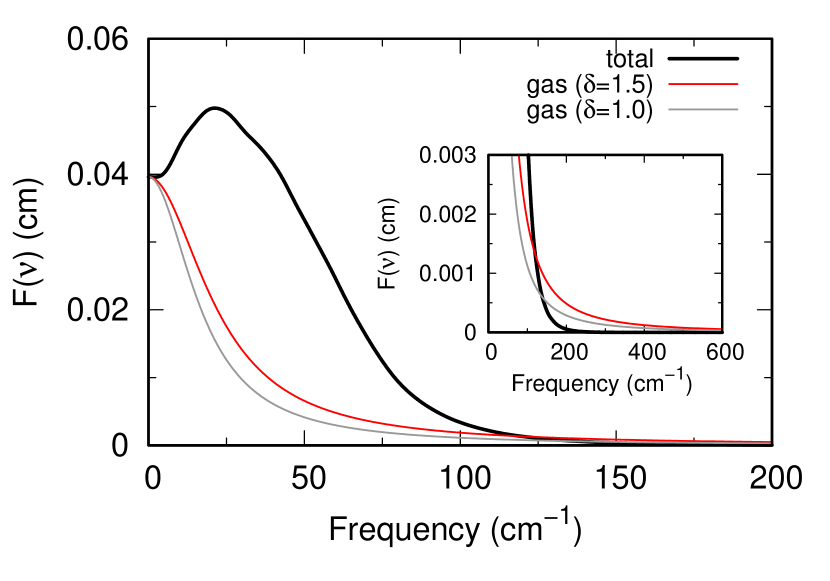
Figure 3: Partitions of the VDoS of liquid argon at $\rho^{\star}=0.85$, $T^{\star}=1.1$ with the gas fraction $f_{g}$ determined from $\delta=1.5$ and $1.0$, respectively. Inset: amplified VDoS demonstrating the high frequency tail $F_{a}(\nu)$.

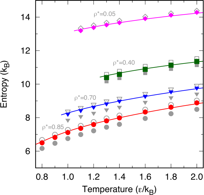
Figure 4: Entropies of liquid argon at various $\rho^{\star}$ and $T^{\star}$. Closed symbols represent predictions from the revised 2PT model with $\delta=1.5$, solid lines are MBWR results, grey open (filled) symbols stand for entropies from the original 2PT model with (without) the $\ln(z)$ term.

To further improve the accuracy of the model, we direct our attention to the gas fraction $f_{g}$, a central parameter in the 2PT model dictating the partition of gas-solid components. As detailed in Appendix A, $f_{g}$ is determined from two assumptions whose theoretical footings are not equal. One is based on the classic Enskog theory of dense HS, while the other, $f_{g}=D/D_{0}$ with $D_{0}$ the diffusivity of dilute HS, is more speculative. It is made under the consideration that $f_{g}$ should be $0$ when the diffusivity of the system is $0$ and approach $1$ in the high temperature-low density limit. Yet this consideration can be served equally well by assuming $f_{g}^{\delta}=D/D_{0}$, where the exponent $\delta$ is not restricted to unity. We emphasize that the original $\delta=1$ may seem natural, but in essence it is a tacit assumption made by Lin et al. and is not required by any physical law. Indeed, if one considers $\tilde{f}_{g}^{\delta}=D/D_{0}$ as the definition of $\delta$, with $\tilde{f}_{g}$ the optimal $f_{g}$ that yields the exact entropy of the system, then $\delta$ will vary from system to system. When the variation of $\delta$ is small, it can be approximated as a constant. At present, we lack physical constraints to compute $\delta$ directly, so its optimal value is determined by comparing with outside references.

After a few tests, we find $\delta=1.5$ a suitable choice for liquid Ar. Partitions of VDoS at $\rho^{\star}=0.85$, $T^{\star}=1.1$ using $\delta=1.5$ as well as the original $\mbox{$\delta$=}1.0$ are shown in Fig. 3. The adoption of $\delta=1.5$ increases $f_{g}$ from $0.35$ to $0.46$ and the packing fraction $\gamma$ from $0.33$ to $0.36$. The corresponding entropy increases from $7.18$ to $7.36$ $k_{B}$ per atom, within $1\%$ of the MBWR value ($7.42$ $k_{B}$). Entropies at other $\rho^{\star}$-$T^{\star}$ conditions are shown in Fig. 4 and tabulated in Table 1 with label “R2PT(1.5)”. We see that the overall agreement with respect to MBWR is quite good, even slightly better than the original 2PT predictions (with the $\ln(z)$ term).

V liquid metals

We now consider an important yet more complex class of fluids: liquid metals. They have broad applications in industryScopigno et al. (2005) as well as in Earth sciences.Belonoshko et al. (2000) Deploying the 2PT model to liquid metals was initiated by Desjarlais,Desjarlais (2013) who proposed a novel memory-function formalism to resolve the perceived overestimation of entropy due to the high frequency tail of $f_{g}F_{g}(\nu)$. However as we noted before, contributions from high frequency tails were not included in Lin et al.’s calculations in the first place, so the actual difference between entropies predicted from the two approaches is minor. Moreover, both approaches rely on the $\ln(z)$ term in the weighting function to produce good results. As we now have a revised 2PT model that works well for liquid Ar, it is tempting to extend this model to liquid metals.

Table 2: Ionic entropies (in $k_{B}$ per atom) of various metals near the experimental melting temperature. Here the density $\rho$ is in g/cm³, temperature $T$ is in Kelvin. “TI” stands for thermodynamic integration. “R2PT ($\delta$)” for the revised 2PT formalism, with the value of $\delta$ in the parentheses. “2PT” and “2PT (w/o $\ln z$)” correspond to results from the original 2PT formalism with and without the $\ln(z)$ term in $W_{g}$. “($n$,  $m$)” denotes the exponents of the Sutton-Chen potential. Uncertainties in the TI and 2PT calculations are estimated to be $0.01$ and $0.02$ $k_{B}$ per atom, respectively.

	$\rho$	$T$	TI	R2PT ($1.5$)	R2PT ($1.0$)	2PT	2PT (w/o $\ln z$)	$(n,\>m)$
Ir	19.0	2700	12.25	12.19	11.99	12.28	11.80	$(14,\>6)$
Ag	9.32	1200	10.24	10.25	10.06	10.33	9.86	$(12,\>6)$
Rh	10.7	2200	11.10	11.09	10.89	11.17	10.68	$(12,\>6)$
Pd	10.38	1800	11.08	11.05	10.84	11.13	10.64	$(12,\>7)$
Au	17.31	1300	11.71	11.73	11.52	11.80	11.29	$(10,\>8)$
Ni	7.81	1700	10.31	10.38	10.17	10.43	9.93	$(9,\>6)$
Al	2.375	900	9.25	9.40	9.20	9.46	8.94	$(7,\>6)$

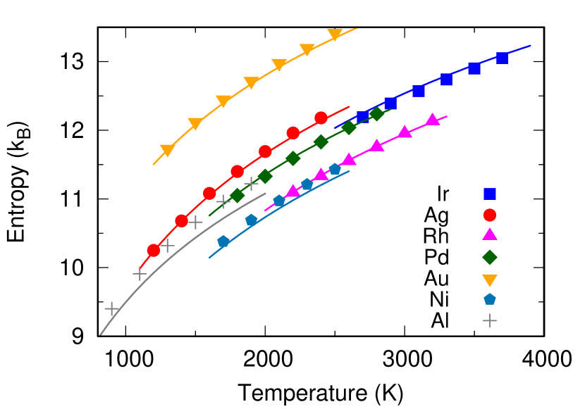
Figure 5: Ionic entropies of liquid metals using the Sutton-Chen potential. Solid lines are references from TI, points are from the revised 2PT model with $\delta=1.5$.

We choose the well-established Sutton-Chen many-atom potentialSutton and Chen (1990) to describe the interatomic interactions in liquid metals. With the Sutton-Chen potential, the total potential energy of the system takes the form

$$U =\epsilon\left[\frac{1}{2}\sum_{i}\sum_{j\neq i}V(r_{ij})-c\sum_{i}\sqrt{\rho_{i}}\right],$$ (14)

where $V(r)=(a/r)^{n}$, $\rho_{i}=\sum_{j\neq i}(a/r_{ij})^{m}$. Among them, $\epsilon$ is a parameter with the dimension of energy, $r_{ij}$ is the separation between atoms $i$ and $j$, $c$ is a positive dimensionless parameter, $a$ is a parameter with the dimension of length, $n$ and $m$ are positive integers. In some respects, the Sutton-Chen potential resembles the Lennard-Jones potential for liquid argon, with $V(r)$ corresponding to the $(\sigma/r)^{12}$ repulsive part and $-c\sqrt{\rho_{i}}$ to the $-(\sigma/r)^{6}$ attractive part. The pair $(n,\>m)$ determines how the potential varies with interatomic distances and serves as a measure of the softness of potentials. To see how our revised model performs with different potentials, we choose seven metals with $(n,\>m)$ ranging from $(14,\>6)$ as Ir, to $(7,\>6)$ as Al.Sutton and Chen (1990) For each metal, we fix its density to the experimental density at melting point $T_{m}$, with temperature ranging from close to $T_{m}$ to $1000$ K above $T_{m}$. The $NVT$ MD simulationsTodorov et al. (2006) were performed in a cubic cell containing $512$ atoms. The time step was $1$ fs. Each simulation first ran $50$ ps for thermal equilibration, then another $100$ ps for production. Calculations of the 2PT model were conducted in the same fashion as in liquid argon. To measure the accuracy of 2PT results, we further performed extensive TI calculations (see Appendix C for details) from which we extract entropies as references.

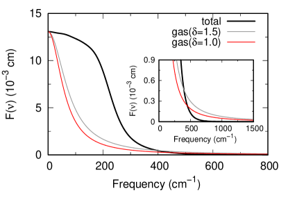
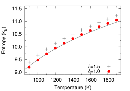
Figure 6: (a) Partitions of VDoS with $\delta=1.5$ and $1.0$ for liquid Al at $\rho=2.375$ g/cm³ and $T=900$ K. Inset: amplified VDoS demonstrating the high frequency tail $F_{a}(\nu)$. (b) Ionic entropies of Al at $\rho=2.375$ g/cm³. Solid lines are references from TI, points are predictions from the revised 2PT model with $\delta=1.5$ and $1.0$, respectively.

Figure 5 compares entropies determined from our revised 2PT model using $\delta=1.5$ with those from TI. The corresponding data are tabulated in Table 2. We see that the overall agreement is good, especially in Ag, Rh, Pd and Au. Still, noticeable discrepancies appear in Ir and Ni, with entropy of the former being underestimated and the latter being overestimated. More significant overestimations are seen in Al. To understand this phenomenon, recall that our revised 2PT model was initially developed for liquid Ar, where the exponent $n\>(m)$ for the repulsive (attractive) part of potential is $12\>(6)$. Apparently, our model works best for liquid metals with $n=12$, such as Ag, Rh, Pd, whereas it underestimates entropy for liquid metals with harder ($n>12)$ potentials and overestimates for those with softer $(n<12)$ potentials. The largest overestimation takes place in Al whose potential is the softest $(n=7)$. In this worst case, the error is $0.15$ $k_{B}$ per atom at $900$ K, or $1.6\%$ of the total ionic entropy. To put this level of accuracy into context, we note the absolute (relative) error at $\rho^{\star}=0.85$, $T^{\star}=0.9$ (near the triple point) is $0.1$ $k_{B}$ ($1.5\%$ ) when the original 2PT model is applied to the Lennard-Jones system.Lin et al. (2003) With $\delta=1.5$ as the default value, our revised 2PT formalism is suited for quick estimations of entropies for a wide range of materials at various conditions, with accuracy comparable to other 2PT formalismsLin et al. (2003); Desjarlais (2013); Meyer et al. (2016) proposed before.

Further improvements in accuracy can be achieved if one does not require a fixed $\delta$ for all materials. From the study of liquid argon, we know that the 2PT entropy relies on the gas-solid partition, and we have introduced a parameter $\delta$ to refine this partition. For Ar, setting $\delta=1.0$ would underestimate entropy while the optimal $\delta=1.5$. This indicates that one may accommodate potentials of different nature by adjusting the parameter $\delta.$ Indeed, take liquid Al as an example, changing $\delta$ from the default value of $1.5$ to $1.0$ yields a smaller gas fraction $f_{g}$, as shown in Fig. 6(a), the resulting entropy also decreases and the agreement with TI gets significantly improved, as shown in Fig. 6(b).

In some situations, quick estimations may not be good enough and one would like to determine the absolute entropy as precise as possible. In principle, TI is the method of choice for such cases. However the computational cost to perform TI can be prohibitively high for AIMD of large systems. In such cases, our revised 2PT model may serve as a viable alternative: one may first perform both the 2PT and TI calculations in a small supercell with fewer atoms at the targeted $T$ and $\rho$, identify the best $\delta$ for this particular thermal state, then apply this $\delta$ to larger supercells. Good transferability of $\delta$ from small to large cells is anticipated since $\delta$ is controlled by interatomic interactions and should not depend strongly on supercell size. This feature can be quite useful for accurate determination of chemical potentials, phase boundaries, etc., for large and complex systems.

VI conclusion

We have conducted a detailed analysis on the 2PT model for computing the ionic entropy of liquids in MD. This analysis reaffirms the seminal idea of Lin, Blanco, and Goddard,Lin et al. (2003) namely, thermodynamic properties of liquids can be accurately determined by decomposition of VDoS using two idealized systems of hard-sphere gas and harmonic oscillators. Some deficiencies in the original model are also identified and addressed. In particular, the spurious $\ln(z)$ term is removed from the weighting function; The correspondence between dynamics and thermodynamics is enforced by considering the VDoS of the gas component as a whole when determining its associated entropy; Partition of gas-solid components is now subject to optimization for better accuracy. With improved theoretical formality, the new formalism is ready to be applied to a wide range of systems for quick entropy estimations. Moreover, it can be combined with TI to obtain accurate entropies of specific thermal states. This latter feature will be useful in situations where high accuracy is necessary, but the systems are too large to perform TI directly.

supplementary material

See supplementary material on the mismatch of HS and total VDoS near $\nu=0$ at high $T$.

Appendix A determination of $f_{g}$

A central parameter in the 2PT model is the gas fraction $f_{g}$ . Equations to determine $f_{g}$ were introduced by Lin et al..Lin et al. (2003) Here we slightly generalize Lin et al.’s approach to improve its applicability.

First, consider that $f_{g}$ should be $0$ when the diffusivity of the system is $0$ (the system is completely solid with no gas fraction) and approach $1$ in the high temperature-low density limit (the system becomes completely gas), thus $f_{g}$ can be defined as

$$f_{g}^{\delta} =\frac{D}{D_{0}(N)},$$ (15)

where $D$ is the diffusivity of the MD system, determined from $F(0)$ using Eq. (3), $D_{0}(N)$ is the diffusivity of HS gas in the low density limit (the Chapman-Enskog result),McQuarrie (2000); Hansen and McDonald (2006) defined as

$$D_{0}(N) =\frac{3}{8}\frac{V}{N\sigma^{2}}\left(\frac{k_{B}T}{\pi m}\right)^{1/2},$$ (16)

with $N$ the total number of particles in the MD system, $V$ the system volume, $m$ the mass of the particle, $\sigma$ the HS diameter, $k_{B}$ the Boltzmann constant. The exponent $\delta$ was set to unity in the original Lin et al.’s paper.Lin et al. (2003) Here we allow it to be system-dependent. Define a normalized diffusivity $\Delta$ as

$$\Delta \equiv\frac{8}{3}(\frac{36}{\pi^{2}})^{1/3}D\sqrt{\frac{\pi m}{k_{B}T}}\left(\frac{N}{V}\right)^{1/3}$$ (17)

and packing fraction $\gamma\equiv\frac{\pi f_{g}N}{6V}\sigma^{3}$, Eq. (15) can be simplified as

$$\gamma =\Delta^{-\frac{3}{2}}f_{g}^{\frac{3}{2}\delta+1}.$$ (18)

The second consideration is that in the spirit of 2PT model, the diffusivity $D$ is solely caused by motions of $f_{g}N$ particles. The rest $(1-f_{g})N$ particles just vibrate and do not diffuse (no contribution to $F(0)$). As such,

$$D_{{\rm HS}}(f_{g}N) =\frac{D}{f_{g}}.$$ (19)

Here $D_{{\rm HS}}(f_{g}N)$ is the diffusivity of HS gas with $f_{g}N$ particles in volume $V$. The $1/f_{g}$ factor on the right-hand side reflects that $D$ is an apparent diffusivity determined from the VACF of $N$ particles, whereas the gas subsystem only contains $f_{g}N$ particles and its actual diffusivity is $1/f_{g}$ times higher than $D$. An analytic theory for $D_{{\rm HS}}$ was given by Enskog as

$$D_{{\rm HS}}(f_{g}N) =D_{0}(f_{g}N)/g(\sigma^{+}),$$ (20)

where $g(\sigma^{+})$ is the value of radial distribution function at contact.Hansen and McDonald (2006) With Carnahan-Starling equation of state, $g(\sigma^{+})=(z-1)/4\gamma$, where the compressibility $z=(1+\gamma+\gamma^{2}-\gamma^{3})/(1-\gamma)^{3}$.Hansen and McDonald (2006) Eq. (19) can be simplified as

$$f_{g}^{2/3} =\frac{\Delta}{2}\frac{\gamma^{2/3}(2-\gamma)}{(1-\gamma)^{3}}.$$ (21)

Substituting $\gamma$ in Eq. (21) using Eq. (18), one reaches the equation for $f_{g}$ as

$$\Delta^{-\frac{9}{2}}f_{g}^{(3+\frac{9\delta}{2})}-3\Delta^{-3}f_{g}^{(3\delta+2)}+3 \Delta^{-\frac{3}{2}}f_{g}^{(1+\frac{3}{2}\delta)}$$

$$-\frac{1}{2}\Delta^{-\frac{3}{2}}f_{g}^{(1+\frac{5}{2}\delta)}+f_{g}^{\delta}-1=0.$$ (22)

For $\delta=1$, the above equation becomes Eq. (34) in Ref. [Lin et al., 2003].

Appendix B excess entropy of hard sphere gas

The excess entropy $S_{{\rm ex}}$ is defined as the entropy difference between non-ideal and ideal gases under the same physical conditions, either identical $T$ and $\rho$ or identical $T$ and $P$.O’Connell and Haile (2005) We first consider identical $T$ and $\rho$, for which

$$S_{{\rm ex}}(T,\>\rho) =S_{{\rm HS}}(T,\>\rho)-S_{{\rm IG}}(T,\>\rho).$$ (23)

$S_{{\rm IG}}(T,\>\rho)$ is described by the Sackur-Tetrode formula as

$$S_{{\rm IG}}(T,\>\rho) =k_{B}[\frac{5}{2}+\frac{3}{2}\ln(\frac{2\pi mk_{B}T}{h^{2}})-\ln(\rho)],$$ (24)

whereas $S_{{\rm ex}}(T,\>\rho)$ is readily determined as follows: consider an isotherm from the present $\rho$ to $\rho\rightarrow 0$ limit as the thermodynamic integration path, we have

$$S_{{\rm ex}}(T,\>\rho) =\int_{0}^{\rho}\frac{d\rho}{\rho^{2}}\left(\beta_{V}^{{\rm IG}}-\beta_{V}^{{\rm HS}}\right),$$ (25)

where $\beta_{V}=(\partial S/\partial V)_{T}=(\partial P/\partial T)_{V}$ is the thermal pressure coefficient. Note as $\rho$ decreases, non-ideal gas becomes increasingly similar to ideal gas, and $S_{{\rm HS}}$ equals $S_{{\rm IG}}$ at the $\rho\rightarrow 0$ limit.

From equation of state $P/\rho k_{B}T=z$, where $z$ is the compressibility ($z=1$ for ideal gas), one finds $\beta_{V}^{{\rm HS}}=z\rho k_{B}$ and $\beta_{V}^{{\rm IG}}=\rho k_{B}$. With Carnahan-Starling equation of stateCarnahan and Starling (1970) $z=(1+\gamma+\gamma^{2}-\gamma^{3})/(1-\gamma)^{3}$ and packing fraction $\gamma=\frac{\pi}{6}\rho\sigma^{3}$, $S_{{\rm ex}}$ is evaluated as

$$S_{{\rm ex}}(T,\>\rho) =k_{B}\int_{0}^{\rho}\frac{d\rho}{\rho}\left(1-z\right)$$

$$=k_{B}\frac{3\gamma^{2}-4\gamma}{(1-\gamma)^{2}}.$$ (26)

To get excess entropy under identical $T$ and $P$, we note that an IG system with density $z\rho$ has the same $P$ as an HS system with density $\rho$. Accordingly,

$$S_{{\rm IG}}(T,\>P) =S_{{\rm IG}}(T,\>z\rho)$$

$$=k_{B}\left[\frac{5}{2}+\frac{3}{2}\ln(\frac{2\pi mk_{B}T}{h^{2}})-\ln(\rho)-\ln z\right].$$ (27)

And the excess entropy

$$S_{{\rm ex}}(T,\>P) =S_{{\rm ex}}(T,\>\rho)+k_{B}\ln z.$$ (28)

Appendix C thermodynamic integration

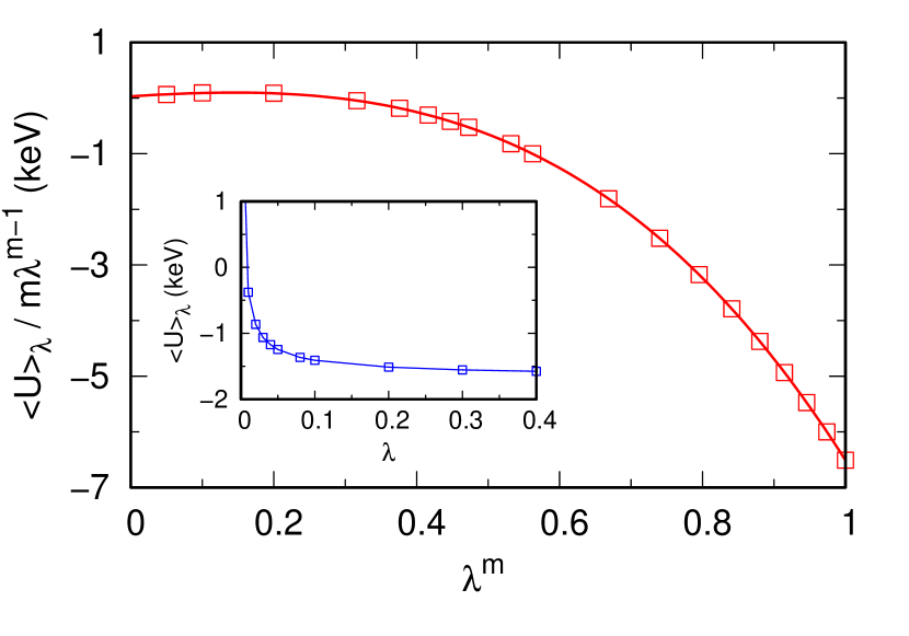
Figure 7: Integrand of TI after transforming $\lambda$ to $\lambda^{m}$ $(m=0.25)$. Squares are data from MD, solid line corresponds to numerical fitting to the fourth order polynomial. Inset: the original integrand $\langle U\rangle_{\lambda}$, which diverges when $\lambda\rightarrow 0$. The target state is liquid Al at $\rho=2.375$ g/cm³, $T=1000$ K.

Thermodynamic integration (TI) is a formally exact method to determine entropy $(S)$ or free energy $(F)$ of a target state. To perform TI, one first choose a reference state whose thermodynamic properties are known; then, a continuous transition path is constructed to connect the reference and target state; finally, $F$ of the target state is obtained by combining that of the reference with the free energy change along the transition path. For a liquid at $(T_{0},\>\rho_{0})$, the reference state is usually set to be ideal gas at $(T_{0},\>\rho_{0})$. The transition path consists of states whose interatomic interactions are gradually switched off.Mezei (1989) Denote the potential energy of the liquid as $U$, states along the transition path as $U_{\lambda}\equiv\lambda U$, where $\lambda$ is the integration variable ranging from $0$ to $1$, we have

$$\frac{\partial F}{\partial\lambda} =\langle\frac{\partial U_{\lambda}}{\partial\lambda}\rangle_{\lambda}$$

$$=\langle U\rangle_{\lambda},$$ (29)

where $\langle\rangle_{\lambda}$ denotes ensemble average with $U_{\lambda}$ being the potential energy of the ensemble. $F$ of the target state is then determined as

$$F =F_{{\rm IG}}+\int_{0}^{1}\langle U\rangle_{\lambda}d\lambda,$$ (30)

where $F_{{\rm IG}}$ is the free energy of ideal gas at $(T_{0},\>\rho_{0})$. This integral is ill-defined because $\langle U\rangle_{\lambda}\rightarrow\infty$ when $\lambda\rightarrow 0$. To remove this divergence at $\lambda=0$, a common practiceMruzik et al. (1976); Mezei (1989) is to transform $\lambda$ to $\lambda^{m}$, such that

$$F =F_{{\rm IG}}+\frac{1}{m}\int_{0}^{1}\frac{\langle U\rangle_{\lambda}}{\lambda^{m-1}}d\lambda^{m}.$$ (31)

Following Ref. [Mruzik et al., 1976] we set $m=0.25$. As shown in Fig. 7, the new integrand is well defined at $\lambda=0$ and the integral can be easily evaluated numerically. Once $F$ is known, $S$($T_{0},\>\rho_{0})$ is evaluated as $S=\left(E-F\right)/T_{0}$. Entropy at other temperatures is determined as

$$S(T,\>\rho_{0}) =S(T_{0},\>\rho_{0})+\int_{T_{0}}^{T}\frac{C_{V}(T^{\prime},\>\rho_{0})}{T^{\prime}}dT^{\prime},$$ (32)

where $C_{V}=(\partial E/\partial T)_{V}$ is the heat capacity at constant volume and can be evaluated from a series of MD simulations with density fixed at $\rho_{0}$ and temperatures sampled between $T_{0}$ and $T$.Sun et al. (2010, 2014)

References

- Allen and Tildesley (1989) M. P. Allen and D. J. Tildesley, Computer simulation of liquids (Oxford University Press, New York, 1989).
- Frenkel and Smit (2002) D. Frenkel and B. Smit, Understanding Molecular Simulation: From Algorithms to Simulations (Academic Press, San Diego, 2002).
- Wallace (1972) D. C. Wallace, Thermodynamics of Crystals (Wiley, New York, 1972).
- Grimvall (1999) G. Grimvall, Thermophysical properties of materials (North-Holland, Amsterdam, 1999).
- Fultz (2010) B. Fultz, Prog. Mater. Sci. 55, 247 (2010).
- Sun et al. (2010) T. Sun, X. Shen, and P. B. Allen, Phys. Rev. B 82, 224304 (2010).
- Zhang et al. (2014) D.-B. Zhang, T. Sun, and R. M. Wentzcovitch, Phys. Rev. Lett. 112, 058501 (2014).
- Sun et al. (2014) T. Sun, D.-B. Zhang, and R. M. Wentzcovitch, Phys. Rev. B 89, 094109 (2014).
- Lu et al. (2017) Y. Lu, T. Sun, P. Zhang, P. Zhang, D.-B. Zhang, and R. M. Wentzcovitch, Phys. Rev. Lett. 118, 145702 (2017).
- Lin et al. (2003) S.-T. Lin, M. Blanco, and W. A. Goddard, J. Chem. Phys. 119, 11792 (2003).
- Huang et al. (2011) S.-N. Huang, T. A. Pascal, I. William A. Goddard, P. K. Maiti, and S.-T. Lin, J. Chem. Theory Comput. 7, 1893 (2011).
- Lin et al. (2010) S.-T. Lin, P. K. Maiti, and I. William A. Goddard, J. Phys. Chem. B 114, 8191 (2010).
- Desjarlais (2013) M. P. Desjarlais, Phys. Rev. E 88, 062145 (2013).
- Robert et al. (2015) G. Robert, P. Legrand, P. Arnault, N. Desbiens, and J. Clérouin, Phys. Rev. E 91, 033310 (2015).
- Jakse and Pasturel (2016) N. Jakse and A. Pasturel, Sci. Rep. 6, 20689 (2016).
- Boates and Bonev (2013) B. Boates and S. A. Bonev, Phys. Rev. Lett. 110, 135504 (2013).
- Carnahan and Starling (1970) N. F. Carnahan and K. E. Starling, J. Chem. Phys. 53, 600 (1970).
- O’Connell and Haile (2005) J. P. O’Connell and J. M. Haile, Thermodynamics: Fundamentals for Applications (Cambridge University Press, Cambridge, 2005).
- Hansen and McDonald (2006) J. P. Hansen and I. R. McDonald, Theory of Simple Liquids, 3rd ed. (Academic Press, Amsterdam, 2006).
- Sutton and Chen (1990) A. P. Sutton and J. Chen, Phil. Mag. Lett. 61, 139 (1990).
- McQuarrie (2000) D. A. McQuarrie, Statistical Mechanics (University Science Books, Sausalito, 2000).
- Berens et al. (1983) P. H. Berens, D. H. J. Mackay, G. M. White, and K. R. Wilson, J. Chem. Phys. 79, 2375 (1983).
- Johnson et al. (1993) J. K. Johnson, J. A. Zollweg, and K. E. Gubbins, Mole. Phys. 78, 591 (1993).
- Todorov et al. (2006) I. T. Todorov, W. Smith, K. Trachenko, and M. T. Dove, J. Mater. Chem. 16, 1911 (2006).
- Press et al. (1986) W. Press, S. Teukolsky, W. Vetterling, and B. Flannery, Numerical Recipes in Fortran 77: The Art of Scientific Computing, 1st ed. (Cambridge University, Cambridge, 1986).
- Scopigno et al. (2005) T. Scopigno, G. Ruocco, and F. Sette, Rev. Mod. Phys. 77, 881 (2005).
- Belonoshko et al. (2000) A. B. Belonoshko, R. Ahuja, and B. Johansson, Phys. Rev. Lett. 84, 3638 (2000).
- Meyer et al. (2016) E. R. Meyer, C. Ticknor, J. D. Kress, and L. A. Collins, Phys. Rev. E 93, 042119 (2016).
- Mezei (1989) M. Mezei, Mol. Simulat. 2, 201 (1989).
- Mruzik et al. (1976) M. R. Mruzik, F. F. Abraham, D. E. Schreiber, and G. M. Pound, J. Chem. Phys. 64, 481 (1976).