Estimating Cosmological Parameters from the Dark Matter Distribution

Abstract

A grand challenge of the 21^st century cosmology is to accurately estimate the cosmological parameters of our Universe. A major approach in estimating the cosmological parameters is to use the large scale matter distribution of the Universe. Galaxy surveys provide the means to map out cosmic large-scale structure in three dimensions. Information about galaxy locations is typically summarized in a “single” function of scale, such as the galaxy correlation function or power-spectrum. We show that it is possible to estimate these cosmological parameters directly from the distribution of matter. This paper presents the application of deep 3D convolutional networks to volumetric representation of dark-matter simulations as well as the results obtained using a recently proposed distribution regression framework, showing that machine learning techniques are comparable to, and can sometimes outperform, maximum-likelihood point estimates using “cosmological models”. This opens the way to estimating the parameters of our Universe with higher accuracy.

1 Introduction

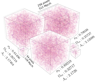
Figure 1: Dark matter distribution in three cubes produced using different sets of parameters. Each cube is divided into small sub-cubes for training and prediction. Note that although cubes in this figure are produced using very different cosmological parameters in our constrained sampled set, the effect is not visually discernible.

The $21^{\mathrm{st}}$ century has brought us tools and methods to observe and analyze the Universe in far greater detail than before, allowing us to deeply probe the fundamental properties of cosmology. We have a suite of cosmological observations that allow us to make serious inroads to the understanding of our own universe, including the cosmic microwave background (CMB) (Planck Collaboration et al., 2015; Hinshaw et al., 2013), supernovae (Perlmutter et al., 1999; Riess et al., 1998) and the large scale structure of galaxies and galaxy clusters (Cole et al., 2005; Anderson et al., 2014; Parkinson et al., 2012). In particular, large scale structure involves measuring the positions and other properties of bright sources in great volumes of the sky. The amount of information is overwhelming, and modern methods in machine learning and statistics can play an increasingly important role in modern cosmology. For example, the common method to compare large scale structure observation and theory is to compare the compressed two-point correlation function of the observation with the theoretical prediction (which is only correct up to a certain physical separation scale). We argue here that there may be a better way to make this comparison.

The best model of the Universe is currently described by less than 10 parameters in the standard $\Lambda$CDM cosmology model, where CDM stands for cold dark matter and $\Lambda$ stands for the cosmological constant. The $\Lambda$CDM parameters that are important for this analysis include the matter density $\Omega_{m}\approx 0.3$ (normal matter and dark matter together constitute $\sim 30\%$ of the energy content of the Universe), the dark energy density $\Omega_{\lambda}\approx 0.7$ ($\sim$70% of the energy content of the Universe is a dark energy substance that pushes the content of the universe apart), the variance in the matter over densities $\sigma_{8}\approx 0.8$ (measured on the matter power spectrum smoothed over 8  $\mathrm{h^{-1}Mpc}$ spheres), and the current Hubble parameter $H_{0}=100h\approx 70\mathrm{km/s/Mpc}$ (which describes the present rate of expansion of the Universe). $\Lambda$CDM also assumes a flat geometry for the Universe, which requires $\Omega_{\Lambda}=1-\Omega_{m}$  (Dodelson, 2003). Note that the unit of distance megaparsec/$h$ ( $\mathrm{h^{-1}Mpc}$ ) used above is time-dependent, where $1\mathrm{Mpc}$ is equivalent to $3.26\times 10^{6}$ light years and $h$ is the dimensionless Hubble parameter that accounts for the expansion of the universe.

The expansion of the Universe stretches the wavelength, or redshifts, the light that is emitted from distant galaxies, with the amount of change in wavelength depending on their distances and the cosmological parameters. Consequently, for a fixed cosmology we can use the directly observed redshift $z$ of galaxies as a proxy for their distance away from us and/or the time at which the light was emitted.

Here, we present a first attempt at using advanced machine learning to predict cosmological parameters directly from the distribution of matter. The final goal is to apply such models to produce better estimates for cosmological parameters in our Universe. In the following, Section 2 presents our main results. Section 3 elaborates on the simulation and cosmological analysis procedures as well as machine learning techniques used to obtain these estimates.

2 Results

To build the computational model, we rely on direct dark matter simulations produced using different cosmological parameters and random seeds. We sample these parameters within a very narrow range that reflects the uncertainty of our current best estimates of these parameters for our universe from real data, in particular the Planck Collaboration et al. (2015) CMB observations. Our objective is to show that it is possible to further improve the estimates in this range, for simulated data, using a deep convolutional neural network (conv-net).

We consider two sets of simulations: the first set contains only one snapshot of the dark matter distribution at the present day. The following cosmological parameters are varied across simulations: I) mass density $\Omega_{m}$; II) $\sigma_{8}$ (or alternatively, the amplitude of the primordial power spectrum, $A_{s}$, which can be used to predict $\sigma_{8}$).

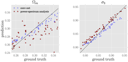
Figure 2: Prediction and ground truth of $\Omega_{m}$ and $\sigma_{8}$ using 3D conv-net and analysis of the power-spectrum on 50 test cube instances.

Here, each training and test instance is the output of an N-body simulation with millions of particles in a box or “cube” that is tens of  $\mathrm{h^{-1}Mpc}$ across. All the simulations in this dataset are recorded at the present day – i.e., redshift $z=0$. Figure 1 shows three cubes with their corresponding cosmological parameters. As is evident from this figure, distinguishing the constants using visual clues is challenging. Importantly, there is substantial variation among cubes even with similar cosmological parameters, since the initial conditions are chosen randomly in each simulation. In all experiments, we use $90\%$ of the data for training and the remaining $10\%$ for testing.

We compare the performance of the conv-net to a standard cosmology analysis based on the standard maximum likelihood fit to the matter power spectrum (Dodelson, 2003). Figure 2 presents our main result, the prediction versus the ground truth for the cosmological parameters using both methods. We find that the maximum likelihood prediction for $(\sigma_{8},\Omega_{m})$ has an average relative error of $(0.013,0.072)$, respectively. In comparison, the conv-net has an average relative error of $(0.012,0.028)$, which has a clear advantage in predicting $\Omega_{m}$. Predictions for conv-net are the mean-value of the predictions on smaller 128  $\mathrm{h^{-1}Mpc}$ sub-cubes. On these sub-cubes, the conv-net has a relatively small standard deviation of $(0.0044,0.0032)$, indicating only small variations in predictions using much smaller sub-cubes. We have not performed a maximum likelihood estimate on these small sub-cubes, since the quality of the results would be drastically limited by sample variance. We also observed that changing the size of these sub-cubes by a factor of two did not significantly affect conv-net’s prediction accuracy; see the Appendix A for details.

The second dataset contains 100 simulations using a more sophisticated simulation code (Trac et al., 2015), where each simulation is recorded at 13 different redshifts $z\in[0,6]$; see Figure 3. Simulations in this set use fewer particles and since the distribution of matter at different redshifts is substantially different (compared to the effect of cosmological parameters in the first dataset) we are able to produce reasonable estimates of the redshift using the distribution-to-real framework of Oliva et al. (2014) as well as a 3D conv-net. Figure 4 reports both results for the training and test sets.

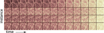
Figure 3: Log-density of dark matter at different redshifts. Each row shows a slice of a different 3D cube. From left to right the redshift increases in $\mathrm{1Gyr}$ steps.

3 Methods

We review the procedure for dark matter simulations in Section 3.1 and outline the standard cosmological likelihood analysis in Section 3.2. Section 3.3 and Section 3.4 detail our deep conv-net applied to the data and our approach to predicting the redshift using a double-basis estimator. Section 3.5 describes the details of the redshift estimation.

3.1 Simulations

Simulations play an important part in modern cosmology studies, particularly in order to model the non-linear effects of general relativity and gravity, which are impossible to take into account in a simpler analytic solution. Consequently, significant effort has been made in the last few decades to obtain a large number of realistic simulations as a function of the cosmology parameters. The simulations also provide a useful test for supervised machine learning techniques.

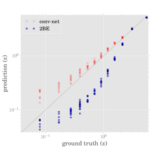
Figure 4: Prediction and ground truth of redshift $z$ on test instances for both 3D conv-net and double-basis estimator (2BE).

In order to apply a Machine Learning process in cosmological parameter estimation we need to generate a huge amount of simulations for the training set. Moreover, it is important to generate big volume simulation boxes in order to accurately reproduce the statistics of large scale structures. There are several algorithms for calculating the gravitational acceleration in N-body simulations, ranging from slow-and-accurate to fast-and-approximate. The equations of motion for the N particles are solved in discrete time steps to track the nonlinear trajectories of the particles.

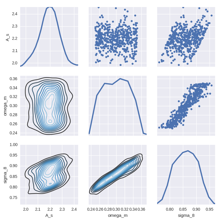
Figure 5: Distribution of cosmological parameters in the first set of simulations.

As we are interested in large scale statistics, for the first dataset we use the COmoving Lagrangian Acceleration (COLA) code (Tassev et al., 2013; Koda et al., 2015). The COLA code is a mixture of N-body simulation and second order Lagrangian perturbation theory. This method conserves the N-body accuracy at large scale and agrees with the non-linear power spectrum (see Section 3.2) that can be obtained with ultra high-resolution pure N-body simulations (Springel, 2005) at better than $95\%$ up to $k\sim 0.5h\mathrm{Mpc^{-1}}$.

For the first study we generate 500 cubic simulations with a size of $512~{}\mathrm{h^{-1}Mpc}~{}$ with $512^{3}$ dark matter particles, evolving the simulation until redshift $z=0$. The mass of these particles varies with the value of $\Omega_{m}$ from $m_{p}\sim 6.5\times 10^{10}$ to $m_{p}\sim 9.5\times 10^{10}\mathrm{h^{-1}M_{\odot}}$, where $M_{\odot}$ is a solar mass. We start the simulations at a redshift of $z\sim 20$ and use 20 steps up to the final redshift $z=0$. Each box is generated using a different seed for the random initial conditions. The Hubble parameter used for all simulations is $H_{0}=70\mathrm{km/s/Mpc}$.

Motivated by the Planck results (Planck Collaboration et al., 2015), we use a Gaussian distribution for the amplitude of the initial scalar perturbations $\ln(10^{10}A_{s})=3.089\pm 0.036$ and a flat distribution in the range $\left[0.25;0.35\right]$ for $\Omega_{m}$. Note that Planck results arguably give us the best constraints on the parameters of our Universe, limiting our simulations mostly to uncertain regions of the parameter space. The value for $\sigma_{8}$ is obtained by calculating the convolution of the linear power spectrum with a top hat window function with a radius of $8~{}\mathrm{h^{-1}Mpc}~{}$, using the Camb code; see Section 3.2 for power-spectrum. Figure 5 shows the distribution of the three parameters (two independent, one derived) that are varying across simulations.

The simulations in the second dataset are based on a particle-particle-particle-mesh ($\mathrm{P^{3}M}$) algorithm from Trac et al. (2015). Each simulation is computed in 13 time steps of 1 gigayear ($\mathrm{Gyr}$), using $128^{3}$ particles in boxes with sizes of 128  $\mathrm{h^{-1}Mpc}$ using the standard $\Lambda CDM$ cosmology.

3.2 Two-Point Correlation and Maximum Likelihood Power Spectrum Analysis

A commonly used measurement for analysis of the distribution of matter is the two-point correlation function $\xi(\vec{r})$, measuring the excess probability, relative to a random distribution, of finding two points in the matter distribution at the volume elements $dV_{1}$ and $dV_{2}$ separated by a vector distance $\vec{r}$ – that is we have

$$dP_{12}(\vec{r})=n^{2}\left(1+\xi(\vec{r})\right)dV_{1}dV_{2},$$ (1)

where $n$ is the mean density (number of particles divided by the volume), and $n^{2}dV_{1}dV_{2}$ in the equation above measures the probability of finding two points in $dV_{1}$ and $dV_{2}$ at vector distance $\vec{r}$. Under the cosmological principle the Universe is statistically isotropic and homogeneous, therefore the correlation function only depends on the distance $r=|\vec{r}|$. The matter power spectrum $P_{m}(k)$ is the Fourier transform of the correlation function, where $k=|\bf k|$ is the magnitude of the Fourier basis vector.

The form of the power spectrum as a function of $k$ depends on the cosmological parameters, in particular $\sigma_{8}$ and $\Omega_{m}$. For a larger (smaller) $\sigma_{8}$ the amplitude of the power spectrum smoothed on the scale of $8~{}\mathrm{h^{-1}Mpc}~{}$ increases (decreases). Similarly, larger $\Omega_{m}$ shifts power into smaller scales.

Given the output of an N-body simulation at $z=0$, we evaluate the “empirical” power spectrum $\hat{P}(k)$ of the dark matter distribution. For a set of cosmological parameters ${Y}=(\sigma_{8},\Omega_{m})$ we can obtain the predicted (theoretical) matter power spectra $P_{m}(k,{Y})$. This theoretical average is produced using our “physical model”, rather than the training data. After obtaining an estimate of the covariance using additional training simulations, for each test cube, we can find the parameter ${Y}$ that maximizes its Gaussian likelihood.

To define this Gaussian likelihood of the empirical power spectra based on its theoretical value $\mathcal{L}(\hat{P}_{m}(k)|P_{m}(k,{Y}))$, we discretize the power spectrum to equally spaced bins in $\log k$. We the estimate the covariance matrix of this Gaussian using 20 different simulations with the fixed cosmology of $(\sigma_{8},\Omega_{m})=(0.812,0.273)$. Note that each of these is using different random initial conditions to obtain an estimate of the sample variance. The sample variance on scales of $k\lesssim 0.1\mathrm{Mpc}$ gives a large uncertainty in the estimate of $\hat{P}_{m}(k)$ at scales $\gtrsim 100~{}\mathrm{h^{-1}Mpc}~{}$ in real-space, which corresponds to approximately $20\%$ of the entire simulation box. This limits the inferences we can draw from large scales in the dark matter simulation.

We then maximize the likelihood function over ${Y}$ using the downhill simplex method (Nelder & Mead, 1965) to obtain an estimate $\hat{}{Y}$ that can be compared to the ground truth cosmological parameter values that are known from the simulations.

3.3 Invariances of the Distribution of Matter

Modern cosmology is built on the cosmological principle that states at large scales, the distribution of matter in the Universe is homogeneous and isotropic (Ryden, 2003), which implies shift, rotation and reflection invariance of the distribution of matter. These invariances have also made the two-point correlation function –as a shift, rotation and reflection invariant measurement– an indispensable tool in cosmological data analysis. Here, we intend to go beyond this measure. Let ${X}$ denote a cube and ${Y}=(\Omega_{m},\sigma_{8})$ the corresponding dependent variable. The existence of invariance in the data means $p({Y}\mid{X})=p({Y}\mid\mathrm{transform}({X}))$, where the invariance identifies the valid transformations.

In machine learning, and in particular deep learning, several recent works have attempted to identify and model the data invariances and its symmetries (e.g.,  Gens & Domingos, 2014; Cohen & Welling, 2014). However, due to inefficiency of current techniques, any known symmetry beyond translation invariance is often enforced by data-augmentation (e.g.,  Krizhevsky et al., 2012); see (Dieleman et al., 2015) for an application in astronomy. Data-augmentation is the process of replicating data by invariant transformations.

In the original representation of cubes, particles are fully interchangable and a source of redundancy is due to this permutation invariance. For conv-nets, prior to data augmentation, we transform this data to volumetric form, where a 3D histogram of $d^{3}$ voxels represents the normalized density of the matter for each cube. For the first and second datasets this resolution (in proportion to the number of particles and the size of these cubes) is set to $d=256$ and $d=64$ respectively, which means each voxel is $2~{}\mathrm{h^{-1}Mpc}~{}$ along each edge. A normalization step ensures that the model generalizes to simulations with different number of particles as long as densities remain non-degenerate. In the first dataset we further break down each of the $500$ simulation cubes to $64^{3}$-voxel sub-cubes, corresponding to $128^{3}(~{}\mathrm{h^{-1}Mpc}~{})^{3}$. This is in order to obtain more training instances for our conv-net; see Figure 1

Translation invariance is addressed by shift-invariance of the convolutional parameters. We augment both datasets with symmetries of a cube. This symmetry group has 48 elements: 6 different $90\text{\,}\mathrm{\SIUnitSymbolDegree}$ rotations and $2^{3}=8$ different axis-reflections of each sub-cube.

The combination of data-augmentation and using “sub”-cubes increases the training data $\mathcal{S}=\{({X}^{(1)},{Y}^{(1)}),\ldots,({X}^{(N)},{Y}^{(N)})\}$ to have $N>10^{6}$ and $N>62000$ instances for the first and second dataset respectively, where in the following we use ${X}\in\Upsilon=\mathbb{R}^{64^{3}}$ to denote a (sub-)cube from either dataset. To see if the data-augmentation has indeed produced the desirable invariance, we predicted both $\Omega_{m}$ and $\sigma_{8}$ using 48 replicates of each sub-cube. The average standard deviation in these predictions is .0013 and .0017 respectively, i.e., small compared to .029 and .039, their respective standard deviations over the whole test-set.

3.4 Deep Convolutional Network for Volumetric Data

Our goal is to learn the model parameters $\theta^{*}\in\Theta$ for an expressive class of functions $\mathsf{f}_{\theta}:\Upsilon\to\mathbb{R}^{2}$, so as to minimize the expected loss $\mathbb{E}_{{X},{Y}}[\ell(\mathsf{f}({X})-{Y})]$ where $\ell(\mathbb{R}^{2})\to\mathbb{R}$ is a loss function — e.g., we use the L1 norm. However, due to the unavailability of $p({X},{Y})$, a common practice is to minimize the empirical loss $\sum_{({X}^{(n)},{Y}^{(n)})\in\mathcal{S}}\ell(\mathsf{f}({X}^{(n)})-{Y}^{(n)})$ with an eye towards generalization to new data, which is often enforced by regularization.

Our function class is the class of a deep convolutional neural network (LeCun et al., 2015; Bengio, 2009). Conv-nets have been mostly applied to 2D image data in the past. Beside applications in video processing –with two image dimensions and time as the third dimension– application of conv-nets to volumetric data are very recent and mostly limited to 3D medical image segmentation (e.g.,  Kamnitsas et al., 2015; Roth et al., 2015).

Figure 6 shows the architecture of our model. A major restriction when moving from 2D images to volumetric data is the substantial increase in the size of the input, which in turn restricts the number of feature-maps at the first layers of the conv-net. This memory usage is further amplified by the fact that in 3D convolution the advantage of using FFT is considerable. However, FFT-based convolution requires larger memory compared to its time domain counterpart.

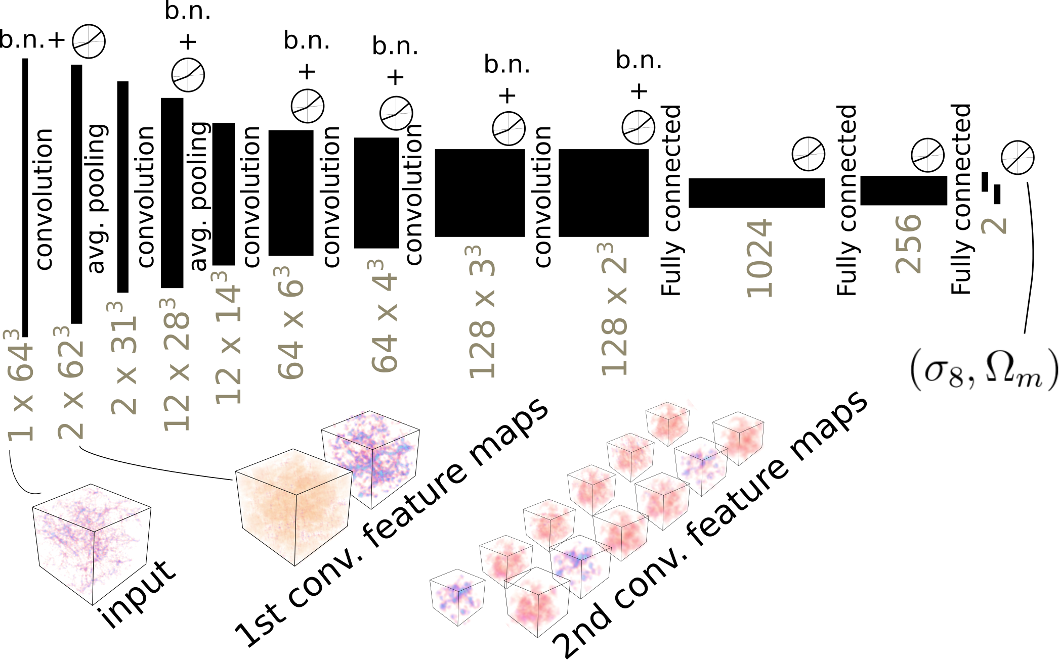
Figure 6: The architecture of our 3D conv-net. The model has six convolutional and 3 fully connected layers. The first two convolutional layers are followed by average pooling. All layers, except the final layer, use leaky rectified linear units, and all the convolutional layers use batch-normalization (b.n.).

In designing our network we identified several choices that are critical in obtaining the results reported in Section 2: I) We use Leaky rectified linear unit (ReLU). (Maas et al., 2013). This significantly speeds up the learning compared to non-leaky variation. We used the leak parameter $c=.01$ in $\mathsf{f}({X})=\max(0,{X})-c$.

II) We used Average pooling in our model and could not learn a meaningful model using max-pooling (which is often used for image processing tasks). One explanation is that with the combination of ReLU and average pooling, activity at higher layers of the conv-net signifies the weighted sum of the dark-matter mass at particular regions of the cube. This information (total mass in a region) is lost when using max-pooling. Here, both pooling layers are sub-sampling by a factor of two along each dimension.

III) Batch normalization (Ioffe & Szegedy, 2015) is necessary to undo the internal covariate shift and stabilize the gradient calculations. The basic idea is to normalize the output of each layer –with an online estimate of mean and variance for all the training data at that layer– before applying the non-linearity.

Regularization is enforced by “drop-out” at fully connected layers, where $50\%$ of units are ignored during each activation, in order to reduce overfitting by preventing co-adaptation (Hinton et al., 2012). For training with backpropagation, we use Adam (Kingma & Ba, 2014) with a learning rate of $.0005$ and first and second moment exponential decay rate of $.9$ and $.999$, respectively.

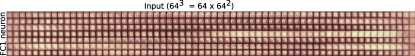
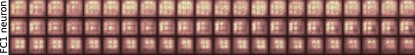
Figure 7: (top) visualization of inputs that maximize the activation of 7/1024 units (corresponding to seven rows) at the first fully connected layer. In this figure, we have unwrapped the maximizing input sub-cubes for better visualization. (bottom) magnified portion of the top row.

3.4.1 Visualization

A common approach to visualizing the representation learned by a deep neural network is to maximize the activation of a particular unit while treating the input ${X}$ as the optimization variable (Erhan et al., 2009; Simonyan et al., 2013)

$${X}^{*}=\arg\max_{{X}}\;s.t.\;{X}_{l,i}\quad\|{X}\|_{2}\leq\zeta$$

where ${X}_{l,i}$ is the $i^{th}$ unit at layer $l$ of the conv-net and $\zeta>0$ is a constant. Figure 7 shows the representation learned by seven units at the first fully connected layer of our model. The visualization suggests that the conv-net has learned to identify various patterns involving periodic concentration of mass as a key feature in predicting $\Omega_{m}$ and $\sigma_{8}$.

3.5 Estimating the Redshift

We applied the conv-net of the previous section to estimate the redshift in our second dataset. Since this is an easier task, we removed two fully connected layers, without losing prediction power. All the other settings in training are kept the same. For this dataset we could also obtain good results using the Double-Basis Estimator, described in the following section.

3.5.1 Distribution to Real Regression

We analyzed the use of distribution-to-real regression (Póczos et al., 2013) and the Double-Basis Estimator (2BE) (Oliva et al., 2014) for predicting cosmological parameters. Here, we take sub-cubes of simulation snapshots to be sample sets from an underlying distribution, and regress a mapping that maps the underlying distribution to a real-value (in this case the redshift of the simulation snapshot). In other words, we consider our data to be $\mathcal{D}=\{(\mathcal{X}_{i},Y_{i})\}_{i=1}^{N}$, where $\mathcal{X}_{i}=\{X_{ij}\in\mathbb{R}^{3}\}_{j=1}^{n_{i}}\overset{iid}{\sim}P_{i}$. We look to estimate a mapping $Y_{i}=f(P_{i})+\epsilon_{i}$, where $\epsilon_{i}$ is a noise term (Oliva et al., 2014).

Roughly speaking, the 2BE operates in an approximate primal space that allows one to use a kernelized estimator on distributions without computing a Gram matrix. The 2BE uses:

I) An orthonormal basis so that we can estimate the $L_{2}$ distance on two distributions, $\lVert P_{i}-P_{j}\rVert_{2}$, as the Euclidean distance of finite vectors of their projection coefficients onto a finite subset of the orthonormal basis, $\lVert\vec{a}(P_{i})-\vec{a}(P_{j})\rVert$.

II) A random basis to approximate kernel evaluations on distributions $K(P_{i},P_{j})$ as the dot product of finite vectors of random features on the respective projection coefficients of the distributions, $z(\vec{a}(P_{i}))^{T}z(\vec{a}(P_{j}))$.

Using these two bases, the 2BE is able to regress a nonparametric mapping efficiently. In short, the 2BE estimates a real valued response, $Y_{i}$, as $Y_{i}\approx\psi^{T}z(\vec{a}(P_{i}))$, where $z(\vec{a}(P_{i}))$ are the aforementioned random features of projection coefficients, and $\psi$ is a vector of model parameters that are optimized over. We expound on the details below.

Orthonormal Basis. We use orthonormal basis projection estimators (Tsybakov, 2008) for estimating densities of $P_{i}$ from a sample $\mathcal{X}_{i}$. Let $\Upsilon=[a,b]$ and suppose that $\Upsilon^{l}\subseteq\mathbb{R}^{l}$ is the domain of input densities. If $\{\varphi_{i}\}_{i\in\mathbb{Z}}$ is an orthonormal basis for $L_{2}(\Upsilon)$, then the tensor product of $\{\varphi_{i}\}_{i\in\mathbb{Z}}$ serves as an orthonormal basis for $L_{2}(\Upsilon^{l})$; that is,

$$\{\varphi_{\alpha}\}_{\alpha\in\mathbb{Z}^{l}}\;\mathrm{where}\;\varphi_{\alpha}(x)=\prod_{i=1}^{l}\varphi_{\alpha_{i}}(x_{i}),\ x\in\Upsilon^{l}$$ (2)

serves as an orthonormal basis (so we have $\forall\alpha,\rho\in\mathbb{Z}^{l},\ \langle\varphi_{\alpha},\varphi_{\rho}\rangle=I{\{\alpha=\rho\}}$).

Let $P\in\mathcal{I}\subseteq L_{2}(\Upsilon^{l})$, then

$$p(x)=\sum_{\alpha\in\mathbb{Z}^{l}}a_{\alpha}(P)\varphi_{\alpha}(x)\ \mathrm{where}$$ (3)

$$\quad a_{\alpha}(P)=\langle\varphi_{\alpha},p\rangle=\int_{\Upsilon^{l}}\varphi_{\alpha}(z)\mathrm{d}P(z)\ \in\mathbb{R}.$$

Here, $p(x)$ denotes the probability density function of the distribution $P$. If the space of input densities, $\mathcal{I}$, is in a Sobolov ellipsoid type space; see (Ingster & Stepanova, 2011; Laurent, 1996; Oliva et al., 2014) for details. We can effectively approximate input densities using a finite set of empirically estimated projection coefficients. Given a sample $\mathcal{X}_{i}=\{X_{i1},\ldots,X_{in_{i}}\}$ where $X_{ij}\overset{iid}{\sim}P_{i}\in\mathcal{I}$, let $\widehat{P}_{i}$ be the empirical distribution of $\mathcal{X}_{i}$; i.e. $\widehat{P}_{i}(X=X_{ij})=\frac{1}{n_{i}}$. Our estimator for $p_{i}$ will be:

$$\tilde{p}_{i}(x)=\sum_{\alpha\in M}a_{\alpha}(\widehat{P}_{i})\varphi_{\alpha}(x)\quad\mathrm{where}$$ (4)

$$a_{\alpha}(\widehat{P}_{i})=\int_{\Upsilon^{l}}\varphi_{\alpha}(z)\mathrm{d}\widehat{P}_{i}(z)=\frac{1}{n_{i}}\sum_{j=1}^{n_{i}}\varphi_{\alpha}(X_{ij}).$$ (5)

Choosing $M$ optimally can be shown to lead to $\mathbb{E}[\lVert\tilde{p}_{i}-p_{i}\rVert_{2}^{2}]=O(n_{i}^{-\frac{2}{2+\gamma^{-1}}})$, where $\gamma^{-1}$ is a smoothing constant (Nussbaum, 1983).

Random Basis. Next, we use random basis functions from Random Kitchen Sinks (RKS) (Rahimi & Recht, 2007) to compute our estimate of the response. In particular, we consider the RBF kernel

$$K_{\delta}(x,y)=\exp\left(-\frac{\lVert x-y\rVert^{2}}{2\delta^{2}}\right)$$

where $x,y\in\mathbb{R}^{d}$ and $\delta\in\mathbb{R}$ is a bandwidth parameter. Rahimi & Recht (2007) shows that for a shift-invariant kernel, such as $K_{\delta}$:

$$K_{\delta}(x,y)\approx z(x)^{T}z(y),\ \mathrm{where}$$ (6)

$$z(x)\equiv\sqrt{\tfrac{2}{D}}\left[\cos(\omega_{1}^{T}x+b_{1})\cdots\cos(\omega_{D}^{T}x+b_{D})\right]^{T}$$ (7)

with $\omega_{i}\stackrel{{\scriptstyle iid}}{{\sim}}\mathcal{N}(0,\delta^{-2}I_{d})$, $b_{i}\stackrel{{\scriptstyle iid}}{{\sim}}\text{Unif}[0,2\pi]$. The quality of the approximation will depend on the number of random features $D$ as well as other factors, see (Rahimi & Recht, 2007) for details.

Below we consider the RBF kernel on distributions,

$$K_{\delta}(P_{i},P_{j})=\exp\left(-\frac{\lVert p_{i}-p_{j}\rVert^{2}}{2\delta^{2}}\right),$$

where $p_{i},p_{j}$ are the respective densities and $\lVert p_{i}-p_{j}\rVert$ is the $L_{2}$ norm on functions. We will take the class of mappings we regress to be:

$$Y_{i}=\sum_{j=1}^{N}\theta_{i}K_{\delta}(G_{j},P_{i})+\epsilon_{i},$$ (8)

where $\lVert\theta\rVert_{1}<\infty$, $G_{j}\in\mathcal{I}$’s are unknown distributions and $\epsilon_{i}$ is a noise term (Oliva et al., 2014). Note that this model is analogous to a linear smoother on some unknown infinite dataset, and is nonparametric. We show that (8) can be approximated with the 2BE below.

Double-Basis Estimator. First note that:

$$\langle\tilde{p}_{i},\tilde{p}_{j}\rangle= \left\langle\sum_{\alpha\in M}a_{\alpha}(\widehat{P}_{i})\varphi_{\alpha},\sum_{\alpha\in M}a_{\alpha}(\widehat{P}_{j})\varphi_{\alpha}\right\rangle$$

$$= \sum_{\alpha\in M}\sum_{\beta\in M}a_{\alpha}(\widehat{P}_{i})a_{\beta}(\widehat{P}_{j})\left\langle\varphi_{\alpha},\varphi_{\beta}\right\rangle$$

$$= \sum_{\alpha\in M}a_{\alpha}(\widehat{P}_{i})a_{\alpha}(\widehat{P}_{j})=\left\langle\vec{a}(\widehat{P}_{i}),\vec{a}(\widehat{P}_{j})\right\rangle,$$

where $\vec{a}(\widehat{P}_{i})=(a_{\alpha_{1}},\ldots,a_{\alpha_{s}})$, $M=\{\alpha_{1},\ldots,\alpha_{s}\}$, and the last inner product is the vector dot product. Thus,

$$\left\lVert\tilde{p}_{i}-\tilde{p}_{j}\right\rVert_{2}=\left\lVert\vec{a}_{t}(\widehat{P}_{i})-\vec{a}_{t}(\widehat{P}_{j})\right\rVert_{2},$$

where the norm on the LHS is the $L_{2}$ norm and the $\ell_{2}$ on the RHS.

Consider a fixed $\delta$. Let $\omega_{i}\stackrel{{\scriptstyle iid}}{{\sim}}\mathcal{N}(0,\delta^{-2}I_{s})$, $b_{i}\stackrel{{\scriptstyle iid}}{{\sim}}\text{Unif}[0,2\pi]$, be fixed. Then,

$$\sum_{i=1}^{\infty}\theta_{i}K_{\delta}(G_{i},P_{0})\approx \sum_{i=1}^{\infty}\theta_{i}K_{\delta}(\vec{a}(G_{i}),\vec{a}(P_{0}))$$

$$\approx \sum_{i=1}^{\infty}\theta_{i}z(\vec{a}(G_{i}))^{T}z(\vec{a}(\widehat{P}_{0}))$$

$$= \left(\sum_{i=1}^{\infty}\theta_{i}z(\vec{a}(G_{i}))\right)^{T}z(\vec{a}_{t}(\widehat{P}_{0}))$$

$$= \psi^{T}z(\vec{a}(\widehat{P}_{0}))$$ (9)

where $\psi=\sum_{i=1}^{\infty}\theta_{i}z(\vec{a}(G_{i}))\in\mathbb{R}^{D}$. Thus, we consider estimators of the form (9). I.e. we use a linear estimator in the non-linear space induced by $z(\vec{a}(\cdot))$. In particular, we consider the OLS estimator using the data-set $\{(z(\vec{a}(\widehat{P}_{i})),Y_{i})\}_{i=1}^{N}$ :

$$\hat{f}(\tilde{P}_{0})\equiv \hat{\psi}^{T}z(\vec{a}(\widehat{P}_{0}))\ \mathrm{where}$$ (10)

$$\hat{\psi}\equiv \operatorname*{arg\,min}_{\beta}\lVert\vec{Y}-{\bf{Z}}\beta\rVert_{2}^{2}=({\bf{Z}}^{T}{\bf{Z}})^{-1}{\bf{Z}}^{T}\vec{Y}$$ (11)

for $\vec{Y}=(Y_{1},\ldots,Y_{N})^{T}$, and with ${\bf{Z}}$ being the $N\times D$ matrix: ${\bf{Z}}=[z(\vec{a}_{t}(\widehat{P}_{1}))\cdots z(\vec{a}_{t}(\widehat{P}_{N}))]^{T}$.

A straightforward extension to (10) is to use a ridge regression estimate on features $z(\vec{a}(\cdot))$ rather than a OLS estimate. That is, for $\lambda\geq 0$ let

$$\hat{\psi}^{T}_{\lambda}\equiv \operatorname*{arg\,min}_{\beta}\lVert\vec{Y}-{\bf{Z}}\beta\rVert_{2}^{2}+\lambda\lVert\beta\rVert_{2}$$ (12)

$$= ({\bf{Z}}^{T}{\bf{Z}}+\lambda I)^{-1}{\bf{Z}}^{T}\vec{Y}.$$ (13)

3.5.2 Algorithm

We summarize the basic steps for training the 2BE in practice given a data-set of empirical functional observations $\mathcal{D}=\{(\mathcal{X}_{i},Y_{i})\}_{i=1}^{N}$, parameters $\delta$ and $D$ (which may be cross-validated), and an orthonormal basis $\{\varphi_{i}\}_{i\in\mathbb{Z}}$ for $L_{2}([a,b])$.

1. Determine the sets of basis functions M for approximating $p$. This may be done via cross validation of density estimates (see (Oliva et al., 2014) for more details).

2. Let $s=|M|$, draw $\omega_{i}\stackrel{{\scriptstyle iid}}{{\sim}}\mathcal{N}(0,\delta^{-2}I_{s})$, $b_{i}\stackrel{{\scriptstyle iid}}{{\sim}}\text{Unif}[0,2\pi]$ for $i\in\{1,\ldots,D\}$; keep the set $\{(\omega_{i},b_{i})\}_{i=1}^{D}$ fixed henceforth.

3. Let $\{\alpha_{1},\ldots,\alpha_{s}\}=M$. Generate the data-set of random kitchen sink features, output projection coefficient vector, response pairs $\{(z(\vec{a}(\widehat{P}_{i})),Y_{i})\}_{i=1}^{N}$. Let $\hat{\psi}=({\bf{Z}}^{T}{\bf{Z}}+\lambda I)^{-1}{\bf{Z}}^{T}\vec{Y}\in\mathbb{R}^{D}$ where ${\bf{Z}}=[z(\vec{a}(\widehat{P}_{1}))\cdots z(\vec{a}(\widehat{P}_{N}))]^{T}\in\mathbb{R}^{N\times D}$, and $\lambda$ may be chosen via cross validation. Note that ${\bf{Z}}^{T}\vec{Y}$ and ${\bf{Z}}^{T}{\bf{Z}}$ can be computed efficiently using parallelism.

4. For all future query input functional observations $\widehat{P}_{0}$, estimate the corresponding response as $\hat{f}(p_{0})=\hat{\psi}^{T}z(\vec{a}(\widehat{P}_{0}))$.

3.6 2BE for Redshift Prediction

We divide simulation snapshots into 16  $\mathrm{h^{-1}Mpc}$ length sub-cubes, for a total of 512 sub-cubes per simulation snapshot. Each sub-cube is then rescaled to be the unit box. We treat each sub-cube as a sample $\mathcal{X}_{i}$ with a response $Y_{i}$, of the redshift it was observed at. In total, a training set of approximately 600K (sample $\mathcal{X}_{i}$, response $Y_{i}$) pairs was used for constructing our model. A total of 130 simulation snapshots were held out. Test accuracies were assessed by averaging the predicted response in the boxes of each held-out snapshot.

We used 20K random features, D, as in Eq. (7). We used the cosine basis, i.e., the tensor product in Eq. (2) of: $\varphi_{0}(x)=1$, and $\varphi_{k}(x)=\sqrt{2}\cos(k\pi x)$ for $k\geq 1$. The set of basis functions, $M$ (5), was taken to be $M=\{\alpha\in\mathbb{N}^{3}\ :\ \lVert\alpha\rVert\leq 18\}$ via rule of thumb. The free parameters $\delta$, the bandwidth, and $\lambda$, the regularizer, were chosen by validation on a held-out portion of the training set. In total the 2BE model’s parameters $\psi$, totaled 20K dimensions.

Future Directions

We demonstrated that machine learning techniques can produce accurate estimates of the cosmological parameters from simulated dark matter distributions, which are highly competitive with standard analysis techniques. In particular the advantage of conv-nets on small-scale boxes shows that convolutional features that carry higher order correlation information provide high fidelity and could produce low variance estimates of the cosmological parameters.

The eventual goal is to use such models to estimate the parameters of our own Universe, where we only have access to the distribution of “visible” matter. This introduces extra complexities as galaxies and clusters are biased tracers of the underlying matter distribution. Furthermore, the direct simulation of galaxy clusters are highly complex. In the next step, we would like to evaluate and establish the robustness of these models to variations across simulation settings, before applying proper models to Sloan Digital Sky Survey data (Alam et al., 2015) that observes the distribution of galaxies at large scales.

Appendix A Spatial Scale of the Cubes

However, increasing the size of cubes comes at the cost of less training/test instances. We evaluated the effect of scale by using different quantizations of the original $512^{3}(~{}\mathrm{h^{-1}Mpc}~{})^{3}$ cubes. The results of Section 2 use a 3D histogram with $256^{3}$ voxels divided into $64^{3}$-voxel sub-cubes. We also tried 3D histograms with $512^{3}$ and $128^{3}$ voxels, with similar $64^{3}$-voxel sub-cubes. We then used the same conv-net for training. This resulted in using $2^{3}=8$ times less or more instances. Figure 8 compares the prediction accuracy under different spatial scales. Error-bars show one standard deviation for the predictions made using different sub-cubes that belong to the same cube (sibling sub-cubes). Interestingly, these predictions for sibling sub-cubes are also consistent, having a small standard deviation for both parameters ($\Omega_{m}$ and $\sigma_{8}$).

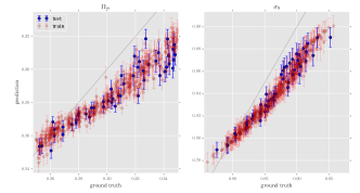
(a) sub-cubic volume of $64^{3}~{}\mathrm{h^{-1}Mpc}~{}$

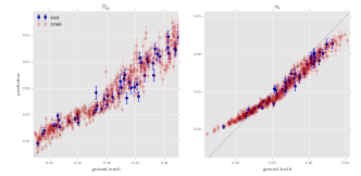
(b) sub-cubic volume of $128^{3}~{}\mathrm{h^{-1}Mpc}~{}$

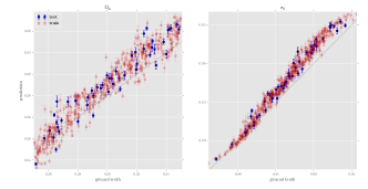
(c) sub-cubic volume of $(256^{3}~{}\mathrm{h^{-1}Mpc}~{}$

Figure 8: Prediction and ground truth using a) small; b) medium and ;c) large sub-cubes. The error-bar shows the standard deviation over predictions made by sibling sub-cubes.

Moreover, change of the spatial volume of sub-cubes does not seem to significantly affect the prediction accuracy. We are able to make predictions with similar accuracy using sub-cubes with both smaller and larger spatial scales.

References

- Alam et al. (2015) Alam, Shadab et al. The Eleventh and Twelfth Data Releases of the Sloan Digital Sky Survey: Final Data from SDSS-III. Astrophys. J. Suppl., 219(1):12, 2015. doi: 10.1088/0067-0049/219/1/12.
- Anderson et al. (2014) Anderson, Lauren et al. The clustering of galaxies in the SDSS-III Baryon Oscillation Spectroscopic Survey: baryon acoustic oscillations in the Data Releases 10 and 11 Galaxy samples. Mon. Not. Roy. Astron. Soc., 441(1):24–62, 2014. doi: 10.1093/mnras/stu523.
- Bengio (2009) Bengio, Yoshua. Learning deep architectures for ai. Foundations and trends in ML, 2(1), 2009.
- Cohen & Welling (2014) Cohen, Taco and Welling, Max. Learning the irreducible representations of commutative lie groups. arXiv preprint arXiv:1402.4437, 2014.
- Cole et al. (2005) Cole, Shaun et al. The 2dF Galaxy Redshift Survey: Power-spectrum analysis of the final dataset and cosmological implications. Mon. Not. Roy. Astron. Soc., 362:505–534, 2005. doi: 10.1111/j.1365-2966.2005.09318.x.
- Dieleman et al. (2015) Dieleman, Sander, Willett, Kyle W, and Dambre, Joni. Rotation-invariant convolutional neural networks for galaxy morphology prediction. Monthly Notices of the Royal Astronomical Society, 450(2):1441–1459, 2015.
- Dodelson (2003) Dodelson, S. Modern Cosmology. Elsevier Science, 2003. ISBN 9780080511979.
- Erhan et al. (2009) Erhan, Dumitru, Bengio, Yoshua, Courville, Aaron, and Vincent, Pascal. Visualizing higher-layer features of a deep network. Dept. IRO, Université de Montréal, Tech. Rep, 4323, 2009.
- Gens & Domingos (2014) Gens, Robert and Domingos, Pedro M. Deep symmetry networks. In Advances in neural information processing systems, pp. 2537–2545, 2014.
- Hinshaw et al. (2013) Hinshaw, G. et al. Nine-Year Wilkinson Microwave Anisotropy Probe (WMAP) Observations: Cosmological Parameter Results. Astrophys. J. Suppl., 208:19, 2013. doi: 10.1088/0067-0049/208/2/19.
- Hinton et al. (2012) Hinton, Geoffrey E, Srivastava, Nitish, Krizhevsky, Alex, Sutskever, Ilya, and Salakhutdinov, Ruslan R. Improving neural networks by preventing co-adaptation of feature detectors. arXiv preprint arXiv:1207.0580, 2012.
- Ingster & Stepanova (2011) Ingster, Y. and Stepanova, N. Estimation and detection of functions from anisotropic sobolev classes. Electronic Journal of Statistics, 5:484–506, 2011.
- Ioffe & Szegedy (2015) Ioffe, Sergey and Szegedy, Christian. Batch normalization: Accelerating deep network training by reducing internal covariate shift. arXiv preprint arXiv:1502.03167, 2015.
- Izard et al. (2015) Izard, A., Crocce, M., and Fosalba, P. ICE-COLA: Towards fast and accurate synthetic galaxy catalogues optimizing a quasi -body method. ArXiv e-prints, September 2015.
- Kamnitsas et al. (2015) Kamnitsas, Konstantinos, Chen, Liang, Ledig, Christian, Rueckert, Daniel, and Glocker, Ben. Multi-scale 3d convolutional neural networks for lesion segmentation in brain mri. Ischemic Stroke Lesion Segmentation, pp. 13, 2015.
- Kingma & Ba (2014) Kingma, Diederik and Ba, Jimmy. Adam: A method for stochastic optimization. arXiv preprint arXiv:1412.6980, 2014.
- Koda et al. (2015) Koda, J., Blake, C., Beutler, F., Kazin, E., and Marin, F. Fast and accurate mock catalogue generation for low-mass galaxies. ArXiv e-prints, July 2015.
- Krizhevsky et al. (2012) Krizhevsky, Alex, Sutskever, Ilya, and Hinton, Geoffrey E. Imagenet classification with deep convolutional neural networks. In Advances in neural information processing systems, pp. 1097–1105, 2012.
- Laurent (1996) Laurent, B. Efficient estimation of integral functionals of a density. The Annals of Statistics, 24(2):659–681, 1996.
- LeCun et al. (2015) LeCun, Yann, Bengio, Yoshua, and Hinton, Geoffrey. Deep learning. Nature, 521(7553):436–444, 2015.
- Lewis & Bridle (2002) Lewis, Antony and Bridle, Sarah. Cosmological parameters from CMB and other data: a Monte- Carlo approach. Phys. Rev., D66:103511, 2002.
- Lewis et al. (2000) Lewis, Antony, Challinor, Anthony, and Lasenby, Anthony. Efficient computation of CMB anisotropies in closed FRW models. Astrophys. J., 538:473–476, 2000.
- Maas et al. (2013) Maas, Andrew L, Hannun, Awni Y, and Ng, Andrew Y. Rectifier nonlinearities improve neural network acoustic models. In Proc. ICML, volume 30, 2013.
- Nelder & Mead (1965) Nelder, John A and Mead, Roger. A simplex method for function minimization. The computer journal, 7(4):308–313, 1965.
- Nussbaum (1983) Nussbaum, M. On optimal filtering of a function of many variables in white gaussian noise. Problemy Peredachi Informatsii, 19(2):23–29, 1983.
- Oliva et al. (2014) Oliva, Junier B, Neiswanger, Willie, Poczos, Barnabas, Schneider, Jeff, and Xing, Eric. Fast distribution to real regression. AISTATS, 2014.
- Parkinson et al. (2012) Parkinson, David et al. The WiggleZ Dark Energy Survey: Final data release and cosmological results. Phys. Rev., D86:103518, 2012. doi: 10.1103/PhysRevD.86.103518.
- Perlmutter et al. (1999) Perlmutter, S. et al. Measurements of Omega and Lambda from 42 high redshift supernovae. Astrophys. J., 517:565–586, 1999. doi: 10.1086/307221.
- Planck Collaboration et al. (2015) Planck Collaboration, Ade, P. A. R., Aghanim, N., Arnaud, M., Ashdown, M., Aumont, J., Baccigalupi, C., Banday, A. J., Barreiro, R. B., Bartlett, J. G., and et al. Planck 2015 results. XIII. Cosmological parameters. ArXiv e-prints, February 2015.
- Póczos et al. (2013) Póczos, Barnabás, Rinaldo, Alessandro, Singh, Aarti, and Wasserman, Larry. Distribution-free distribution regression. AISTATS, 2013.
- Rahimi & Recht (2007) Rahimi, Ali and Recht, Benjamin. Random features for large-scale kernel machines. Advances in neural information processing systems, pp. 1177–1184, 2007.
- Riess et al. (1998) Riess, Adam G. et al. Observational evidence from supernovae for an accelerating universe and a cosmological constant. Astron. J., 116:1009–1038, 1998. doi: 10.1086/300499.
- Roth et al. (2015) Roth, Holger R, Farag, Amal, Lu, Le, Turkbey, Evrim B, and Summers, Ronald M. Deep convolutional networks for pancreas segmentation in ct imaging. In SPIE Medical Imaging, pp. 94131G–94131G. International Society for Optics and Photonics, 2015.
- Ryden (2003) Ryden, Barbara Sue. Introduction to cosmology, volume 4. Addison-Wesley San Francisco USA, 2003.
- Simonyan et al. (2013) Simonyan, Karen, Vedaldi, Andrea, and Zisserman, Andrew. Deep inside convolutional networks: Visualising image classification models and saliency maps. arXiv preprint arXiv:1312.6034, 2013.
- Smith et al. (2003) Smith, R. E., Peacock, J. A., Jenkins, A., White, S. D. M., Frenk, C. S., Pearce, F. R., Thomas, P. A., Efstathiou, G., and Couchmann, H. M. P. Stable clustering, the halo model and nonlinear cosmological power spectra. Mon. Not. Roy. Astron. Soc., 341:1311, 2003. doi: 10.1046/j.1365-8711.2003.06503.x.
- Springel (2005) Springel, V. The cosmological simulation code GADGET-2. mnras, 364:1105–1134, December 2005. doi: 10.1111/j.1365-2966.2005.09655.x.
- Tassev et al. (2013) Tassev, S., Zaldarriaga, M., and Eisenstein, D. J. Solving large scale structure in ten easy steps with COLA. jcap, 6:036, June 2013. doi: 10.1088/1475-7516/2013/06/036.
- Trac et al. (2015) Trac, H., Cen, R., and Mansfield, P. SCORCH I: The Galaxy-Halo Connection in the First Billion Years. apj, 813:54, November 2015. doi: 10.1088/0004-637X/813/1/54.
- Tsybakov (2008) Tsybakov, Alexandre B. Introduction to nonparametric estimation. Springer, 2008.