Local pressure for confined systems

Abstract

We derive a general closed expression for the local pressure exerted onto the corrugated walls of a channel confining a fluid medium. When the fluid medium is at equilibrium the local pressure is a functional of the shape of the walls. It is shown that, due to the intrinsic non-local character of the interactions among the particles forming the fluid, the applicability of approximate schemes such as the concept of a surface of tension or morphometric thermodynamics is limited to wall curvatures small compared to the range of particle-particle interactions.

I Introduction

In a variety of scenarios, such as biological systems Alberts et al. (2007), micro- and nano-fluidic circuitry Duncombe et al. (2015), and energy harvesting devices Wang and Wu (2012), physical systems are composed of a fluid medium confined by means of solid or liquid interfaces. Clearly, the confining walls affect both the dynamics and the steady states of the fluid medium due to the additional interactions between the fluid phase and the boundaries. For example, droplet formation Bakker (1908), electric charge accumulation in confined electrolytes Frenkel (1901), and active particle accumulation in microchannels Rothschild (1963) are driven by the effective interactions between the otherwise unbounded fluid medium and the confining walls. In order to grasp the effect of the presence of the confining walls on the dynamics of confined fluids, up to now, the attention has been focused on the case of fluid media embedded between parallel plates or in channels with constant cross-sections. However, many experimentally relevant cases are not covered by these geometries. For example, porous materials, microfluidic devices, or biological scenarios, are characterized by larger cavities that alternate with narrow bottlenecks. This inhomogeneity in the confining space couples to the dynamics of the confined systems possibly leading to novel scenarios. Indeed, electrolytes confined in varying section pores have been observed to undergo novel regimes Kalman et al. (2008); Malgaretti et al. (2014); Laohakunakorn and Keyser (2015); Melnikov et al. (2017); Dubov et al. absent in the corresponding unbound scenarios. Similarly both passive Reguera and Rubí (2001); Dagdug et al. (2011, 2012); Reguera et al. (2012); Marini Bettolo Marconi et al. (2015); Malgaretti et al. (2016) and active Di Leonardo et al. (2010); Malgaretti et al. (2012); Ghosh et al. (2013); Sandoval and Dagdug (2014); Malgaretti and Stark (2017) colloidal particles as well as polymers Wong and Muthukumar (2008); Nikoofard and Fazli (2011); Nedelcu and Sommer (2013); Bianco and Malgaretti (2016); Datar et al. display confinement-induced dynamical regimes when embedded within varying section channels. In order to unravel the the general mechanisms responsible of these diverse phenomena, it is of primary importance to understand the physical origin of the effective coupling between the fluid medium and the confining walls. Accordingly, an insight into such a coupling can be provided by the knowledge of the dependence of local intensive thermodynamic quantities, e.g., pressure, on the local geometry of the confining walls. Indeed local imbalances in such quantities will lead to net local fluxes that are tuned by the geometry of the confining walls. Alternatively, imposing the equilibrium condition, i.e., constancy of intensive thermodynamic variables, will provide insight into the rearrangement of the fluid medium under inhomogeneous confining conditions.

In the following, we derive a framework capable of capturing the local dependence of thermodynamic variables of the embedded fluid medium, and we derive a general expression for the local pressure exerted onto the confinement. To that end, the fluid medium is described in terms of density functional theory (DFT), which is in principle exact Evans (1979) and for which numerous considerably precise approximation schemes have been developed in the past Tarazona (1984, 1985); Rosenfeld (1989); Roth et al. (2002); Wittmann et al. (2016). Accordingly, our closed expression for the local pressure is exact within this framework.

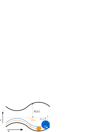
Figure 1: Cartoon of the system under study. Particles (depicted as discs) are confined to the interior of a channel whose upper and lower walls are located respectively at $z=h_{+}(x)$ and $z=-h_{-}(x)$. Due to their radius $R_{\alpha}$, the volume accessible to particles of species $\alpha$ is given by $z\in[-H_{\alpha}^{-}(x),H_{\alpha}^{+}(x)]$. A particle of species $\alpha$ located at position $(x,\pm H_{\alpha}^{\pm}(x))$ touches the wall at point $(\bar{x}^{\pm}_{\alpha}(x,[h_{\pm}]),h_{\pm}(\bar{x}^{\pm}_{\alpha}(x,[h_{\pm}])))$.

The structure of the text is the following. In Sec. II we define the model (Sec. II.1), set up the DFT approach (Sec. II.2), and derive a closed expression for the local pressure (Sec. II.3). In order to demonstrate the application of the general form of the local pressure derived in Sec. II, we discuss our results in the context of the concept of a surface of tension and in comparison with the approach of morphometric thermodynamics in Sec. III. Finally in Sec. IV we give some concluding remarks.

II General formalism

II.1 Model

As sketched in Fig. 1, consider in the three-dimensional Euclidean space an $s$-component mixture which is confined by two hard walls

$$\mathcal{W}_{+}[h_{+}]:= \{(x,y,z)\in\mathbb{R}^{3}\ |\ z>\phantom{-}h_{+}(x)\}$$ (1a)

$$\mathcal{W}_{-}[h_{-}]:= \{(x,y,z)\in\mathbb{R}^{3}\ |\ z<-h_{-}(x)\}\,,$$ (1b)

where the positive real functions $h_{\pm}:\mathbb{R}\to(0,\infty)$ describe the wall shapes. The particles of species $\alpha\in\{1,\dots,s\}$ possess a spherical hard core of radius $R_{\alpha}\geq 0$, and, due to the hard walls $\mathcal{W}_{+}[h_{+}]$ and $\mathcal{W}_{-}[h_{-}]$, they are confined to the interior of the accessible volume $\mathcal{V}_{\alpha}[h]:=\{(x,y,z)\in\mathbb{R}^{3}\ |\ -H^{-}_{\alpha}(x,[h_{-}])<z<H^{+}_{\alpha}(x,[h_{+}])\}$ with the positive real functions $H^{\pm}_{\alpha}[h_{\pm}]:\mathbb{R}\to(0,\infty)$. Here and in the following $h:=(h_{+},h_{-})$ is an abbreviation of the set of both wall shape functions $h_{+}$ and $h_{-}$. In order to have the functions $H^{\pm}_{\alpha}[h_{\pm}]$, which describe the boundary $\partial\mathcal{V}_{\alpha}[h]$ of the accessible volume $\mathcal{V}_{\alpha}[h]$, being well-defined, the radii of curvature $R^{\pm}_{\text{w}}(x,[h_{\pm}]):=(1+h_{\pm}^{\prime}(x)^{2})^{3/2}/h_{\pm}^{\prime\prime}(x)$ of the walls are required to be larger than the radius of all particles: $|R^{\pm}_{\text{w}}(x)|>R_{\alpha}$ for all $x\in\mathbb{R}$ and $\alpha\in\{1,\dots,s\}$. Besides the hard-core interactions, additional fluid-fluid and fluid-wall interactions can be present. The structure of the fluid is described in terms of the number density profiles $\varrho_{\alpha}$ of species $\alpha\in\{1,\dots,s\}$, which, due to the translational invariance of the system along the $y$-direction, can be assumed to depend only on $x$ and $z$. The hard-core interaction precludes particles of species $\alpha\in\{1,\dots,s\}$ to be found outside the accessible volume $\mathcal{V}_{\alpha}$, i.e., $\varrho_{\alpha}(x,z)=0$ for $(x,y,z)\not\in\mathcal{V}_{\alpha}[h]$.

II.2 Density functional theory

Without restriction of generality the grand-canonical density functional describing the fluid is given by

$$\beta\Omega\left[\underline{\varrho},h\right]=\mathcal{A}\left[\underline{\varrho},\underline{H}^{+}[h_{+}],\underline{H}^{-}[h_{-}],h\right]$$ (2)

with the auxiliary functional

$$\mathcal{A}\left[\underline{\varrho},\underline{J}^{+},\underline{J}^{-},h\right]=L_{y}\int\!\mathrm{d}x\sum_{\alpha=1}^{s}\int\limits_{-J^{-}_{\alpha}(x)}^{J^{+}_{\alpha}(x)}\!\!\!\!\!\mathrm{d}z\;\varrho_{\alpha}(x,z)\left[f_{\alpha}\left(\varrho_{\alpha}(x,z)\right)-\beta\mu_{\alpha}+\beta V_{\alpha}(x,z,[h])\right]+\beta F^{\text{ex}}\left[\underline{\varrho},\underline{J}^{+},\underline{J}^{-}\right],$$ (3)

where $\underline{\varrho}=(\varrho_{1},\dots,\varrho_{s})$ denotes the set of all density profiles and similarly for other quantities, and $L_{y}$ is the thickness of the system along the $y$ direction. In Eq. (3), $V_{\alpha}(x,z,[h])$ and $\mu_{\alpha}$ are respectively the particle-wall interaction in excess to the hard-core interaction for particles of species $\alpha\in\{1,\dots,s\}$ and the chemical potential. Note that $V_{\alpha}(x,z,[h])$ depends explicitly on the shapes $h_{+}$ and $h_{-}$ of the confining walls. The reference system is described by the free energy density per particle $f_{\alpha}(\varrho_{\alpha})$, which equals exactly $\ln(\varrho_{\alpha}\Lambda^{3}_{\alpha})-1$ with the thermal wave length $\Lambda_{\alpha}$ for the case of an ideal gas, but which also allows for a description within a local density approximation (LDA). In the present work the free energy functional $F^{\text{ex}}$ in excess to the reference functional is chosen of the rather general form

$$\beta F^{\text{ex}}\left[\underline{\varrho},\underline{J}^{+},\underline{J}^{-}\right]$$

$$= -L_{y}\!\sum_{n=2}^{\infty}\frac{1}{n!}\sum_{\alpha_{1},\dots,\alpha_{n}=1}^{s}\int\!\mathrm{d}x_{1}\!\!\!\!\!\!\!\!\int\limits_{-J^{-}_{\alpha_{1}}(x_{1})}^{J^{+}_{\alpha_{1}}(x_{1})}\!\!\!\!\!\!\!\mathrm{d}z_{1}\dots\int\!\mathrm{d}x_{n}\!\!\!\!\!\!\!\!\int\limits_{-J^{-}_{\alpha_{n}}(x_{n})}^{J^{+}_{\alpha_{n}}(x_{n})}\!\!\!\!\!\!\!\mathrm{d}z_{n}\;c_{\alpha_{1}\dots\alpha_{n}}^{(0)}(x_{1},z_{1},\dots,x_{n},z_{n})\varrho_{\alpha_{1}}(x_{1},z_{1})\cdots\varrho_{\alpha_{n}}(x_{n},z_{n}).$$ (4)

All weighted density approximations (WDA), including the fundamental measure theories (FMT), are of this form. However, gradient expansions, such as the well-known square-gradient approximation within the Cahn-Hilliard approach, cannot be represented in the form of Eq. (4).

Given some wall shapes $h$, the equilibrium number density profiles $\varrho^{\text{eq}}[h]$ are solutions of the Euler-Lagrange equations

$$0 =\frac{\delta\beta\Omega}{\delta\varrho_{\alpha}(x,z)}[\underline{\varrho}^{\text{eq}}[h],h]$$

$$=\frac{\delta\mathcal{A}}{\delta\varrho_{\alpha}(x,z)}[\underline{\varrho}^{\text{eq}}[h],\underline{H}^{+}[h_{+}],\underline{H}^{-}[h_{-}],h]$$ (5)

for all $\alpha\in\{1,\dots,s\}$ and $(x,y,z)\in\mathcal{V}_{\alpha}[h]$.

II.3 Deformation work and local pressure

When the fluid medium is at equilibrium, or in some non-equilibrium steady state, the conditions of the system, composed of the walls and the fluid medium, are such that the state of the fluid medium, represented by the density profiles $\underline{\varrho}$, is determined by the shapes of the walls $h_{\pm}$ alone: $\underline{\varrho}=\underline{\varrho}^{*}[h]$. In such a scenario one obtains from Eq. (2) the effective wall Hamiltonian on the function space of all wall shapes $h=(h_{+},h_{-})$

$$\beta\Xi[h]:=\beta\Omega\left[\underline{\varrho}^{*}[h],h\right]$$ (6)

that represents the energy of the system for given wall shapes $h$.

In the following, we restrict ourselves to the case of the fluid medium being at equilibrium, i.e., $\underline{\varrho}^{*}=\underline{\varrho}^{\text{eq}}$, where the equilibrium state is given by Eq. (5). In such a condition Eq. (6) reads

$$\beta\Xi[h]=\beta\Omega\left[\underline{\varrho}^{\text{eq}}[h],h\right],$$ (7)

and the degrees of freedom of the fluid medium are accounted for in terms of the equilibrium state $\underline{\varrho}^{\text{eq}}[h]$.

Accordingly, as is shown in detail in Appendix A, the work needed to deform the walls $h=(h_{+},h_{-})$ by $\delta h=(\delta h_{+},\delta h_{-})$ is given by

$$\delta\beta\Xi\left[h,\delta h\right] =L_{y}\int\!\mathrm{d}x^{\prime}\sum_{\alpha=1}^{s}\sum_{t\in\{\pm\}}\!\!\Bigg{[}-\partial_{x^{\prime}}K^{t}_{\alpha}(x^{\prime},[h_{t}])\left.\varrho_{\alpha}^{\text{eq}}(x,tH^{t}_{\alpha}(x,[h_{t}]),[h])^{2}f_{\alpha}^{\prime}(\varrho_{\alpha}^{\text{eq}}(x,tH^{t}_{\alpha}(x,[h_{t}]),[h]))\right|_{x=K^{t}_{\alpha}(x^{\prime},[h_{t}])}$$

$$\phantom{=L_{y}\int\!\mathrm{d}x^{\prime}\sum_{\alpha=1}^{s}\sum_{t\in\{\pm\}}\!\!\Bigg{[}}+\int\!\mathrm{d}x\int\limits_{-H^{-}_{\alpha}(x,[h_{-}])}^{H^{+}_{\alpha}(x,[h_{+}])}\!\!\!\mathrm{d}z\;\varrho_{\alpha}^{\text{eq}}(x,z,[h])\frac{\delta\beta V_{\alpha}}{\delta h_{t}(x^{\prime})}(x,z,[h])\Bigg{]}\ \delta h_{t}(x^{\prime}),$$ (8)

where (compare Eq. (50) in Appendix A)

$$K^{\pm}_{\alpha}(x^{\prime},[h_{\pm}]):=x^{\prime}+\frac{R_{\alpha}h_{\pm}^{\prime}(x^{\prime})}{\sqrt{1+h_{\pm}^{\prime}(x^{\prime})^{2}}}.$$ (9)

Equation (8) is an expression of the work $\beta\Xi[h,\delta h]$ required to deform the walls, whose shape is described by $h=(h_{+},h_{-})$, such that $h$ is changed by $\delta h$. It is of the form

$$\delta\Xi\left[h,\delta h\right]=-L_{y}\int\!\mathrm{d}x\left[\beta P^{+}_{z}(x,[h])\ \delta h_{+}(x)+\beta P^{-}_{z}(x,[h])\ \delta h_{-}(x)\right]$$ (10)

where

$$\beta P^{t}_{z}(x,[h]) =\sum_{\alpha=1}^{s}\Bigg{[}\partial_{x}K^{t}_{\alpha}(x,[h_{t}])\left.\varrho_{\alpha}^{\text{eq}}(x^{\prime},tH^{t}_{\alpha}(x^{\prime},[h_{t}]),[h])^{2}f_{\alpha}^{\prime}(\varrho_{\alpha}^{\text{eq}}(x^{\prime},tH^{t}_{\alpha}(x^{\prime},[h_{t}]),[h]))\right|_{x^{\prime}=K^{t}_{\alpha}(x,[h_{t}])}\$$

$$\phantom{=\sum_{\alpha=1}^{s}\Bigg{[}}-\int\!\mathrm{d}x^{\prime}\int\limits_{-H^{-}_{\alpha}(x^{\prime},[h_{-}])}^{H^{+}_{\alpha}(x^{\prime},[h_{+}])}\!\!\!\mathrm{d}z^{\prime}\;\varrho_{\alpha}^{\text{eq}}(x^{\prime},z^{\prime},[h])\frac{\delta\beta V_{\alpha}}{\delta h_{t}(x)}(x^{\prime},z^{\prime},[h])\Bigg{]}$$ (11)

is the local force along the positive ($t=+$) or negative ($t=-$) $z$-direction per unit area projected onto the axis of the channel the fluid exerts on the walls at $(x,y,th_{t}(x))$. Using as reference system in Eq. (3) the ideal gas with free energy per particle $f_{\alpha}(\varrho_{\alpha})=\ln(\varrho_{\alpha}\Lambda_{\alpha}^{3})-1$ one obtains $\varrho_{\alpha}^{2}f^{\prime}_{\alpha}(\varrho_{\alpha})=\varrho_{\alpha}$, so that Eq. (11) simplifies to

$$\beta P^{t}_{z}(x,[h]) =\sum_{\alpha=1}^{s}\Bigg{[}\partial_{x}K^{t}_{\alpha}(x,[h_{t}])\varrho_{\alpha}^{\text{eq}}(K^{t}_{\alpha}(x,[h_{t}]),tH^{t}_{\alpha}(K^{t}_{\alpha}(x,[h_{t}]),[h_{t}]),[h])$$

$$\phantom{=\sum_{\alpha=1}^{s}\Bigg{[}}-\int\!\mathrm{d}x^{\prime}\int\limits_{-H^{-}_{\alpha}(x^{\prime},[h_{-}])}^{H^{+}_{\alpha}(x^{\prime},[h_{+}])}\!\!\!\mathrm{d}z^{\prime}\;\varrho_{\alpha}^{\text{eq}}(x^{\prime},z^{\prime},[h])\frac{\delta\beta V_{\alpha}}{\delta h_{t}(x)}(x^{\prime},z^{\prime},[h])\Bigg{]}.$$ (12)

The rotation invariance of $P^{t}_{z}$ (see Appendix B) allows one to determine the local force $P^{t}_{x}(x,[h])$ along the $x$-direction per unit area projected onto the axis of the channel the fluid exerts on the walls at $(x,y,th_{t}(x))$. By definition the force exerted on a surface element of the wall at point $(x,y,th_{t}(x))$ with rectangular projection of size $\mathrm{d}x$ and $L_{y}$ onto the $x$-$y$ plane is given by $(P^{t}_{x}(x,[h]),tP^{t}_{z}(x,[h]))L_{y}\mathrm{d}x$. As the force is a vectorial quantity, it transforms upon rotation $T(\varphi)$ with the rotation matrix $\mathbb{T}(\varphi)$:

$$\left(\begin{array}[]{c}P^{t}_{x}(\tilde{x},[\tilde{h}])\\ tP^{t}_{z}(\tilde{x},[\tilde{h}])\end{array}\right)L_{y}\mathrm{d}\tilde{x}=\mathbb{T}(\varphi)\left(\begin{array}[]{c}P^{t}_{x}(x,[h])\\ tP^{t}_{z}(x,[h])\end{array}\right)L_{y}\mathrm{d}x.$$ (17)

Substituting $z=th_{t}(x)$ in Eq. (58) and forming the differential of the first component one obtains the expression $\mathrm{d}\tilde{x}=(\cos\varphi-\sin\varphi th_{t}^{\prime}(x))\mathrm{d}x$. Using this relation as well as Eq. (62) one infers from the second component in Eq. (17) the expression $P^{t}_{x}(x,[h])=-h_{t}^{\prime}(x)P^{t}_{z}(x,[h])$, and hence the force onto a surface element of the wall (see Eq. (17)) is given by

$$\left(\begin{array}[]{c}P^{t}_{x}(x,[h])\\ tP^{t}_{z}(x,[h])\end{array}\right)L_{y}\mathrm{d}x =P^{t}_{z}(x,[h])\left(\begin{array}[]{c}-h_{t}^{\prime}(x)\\ t\end{array}\right)L_{y}\mathrm{d}x$$ (22)

$$=P^{t}_{z}(x,[h])\mathbf{n}_{t}(x,[h_{t}])\mathrm{d}\mathcal{A},$$ (23)

where $\mathbf{n}_{t}(x,[h_{t}])=(-h_{t}^{\prime}(x),t)/\sqrt{1+h_{t}^{\prime}(x)^{2}}$ is the outer normal vector of the wall at $(x,y,h_{t}(x))$ and $\mathrm{d}\mathcal{A}=L_{y}\sqrt{1+h_{t}^{\prime}(x)^{2}}\mathrm{d}x$ is the size of the surface element. Therefore, in agreement with the intuitive expectation that a fluid in equilibrium cannot sustain shear, the force the fluid medium is exerting onto the walls acts in normal direction. Moreover, the quantities $P^{t}_{z}$ in Eqs. (11) and (12) represent the force per wall area, i.e., the local pressure. Therefore Eqs. (11) and (12) can be seen as a local version of the so-called “contact theorems” which, so far, consider effectively averages of the wall density, either due to the symmetry at regularly formed walls Lebowitz (1960); Henderson et al. (1979); Henderson (1983); Podgornik (1993); Mallarino et al. (2015) or as explicit averages along arbitrarily-shaped walls Upton (1998).

III Discussion

III.1 Sum rules

Some general statements concerning the local pressures $P_{z}^{\pm}(x,[h])$ can inferred directly from the expression for the mechanical work, Eq. (10), without the need to determine the equilibrium density profiles $\varrho_{\alpha}^{\text{eq}}$. The work required to induce the deformation $\delta h=(\delta h_{+},\delta h_{-})$ of the channel walls in general reads

$$\delta\Xi=-p\delta\mathcal{V}+\bar{\gamma}_{+}\delta\mathcal{A}_{+}+\bar{\gamma}_{-}\delta\mathcal{A}_{-},$$ (24)

where $\delta\mathcal{V}$ and $\delta\mathcal{A}_{\pm}$ are respectively the changes in volume and in surface areas due to the deformation $\delta h$ of the walls, $p$ is the bulk pressure, and $\bar{\gamma}_{\pm}$ are the associated interfacial tensions. For the special case of deformations $\delta h$ leaving the size of the surface areas unchanged,

$$\begin{cases}\delta\mathcal{V}&\neq 0\\ \delta\mathcal{A}_{\pm}&=0,\end{cases}$$ (25)

the total work depends solely on the “bulk” contribution $\sim\delta\mathcal{V}$ on the right-hand side of Eq. (24). Comparing Eq. (24) to Eq. (10) under these conditions one infers the sum rule

$$\int\!\mathrm{d}x(P^{\pm}_{z}(x,[h])-p)\ \delta h_{\pm}(x)=0\,.$$ (26)

In particular, when the walls are deformed uniformly, i.e., $\delta h_{\pm}(x)$ does not depend on the position $x$ along the channel, one obtains from Eq. (26) the sum rule

$$\int\!\mathrm{d}x(P^{\pm}_{z}(x,[h])-p)=0$$ (27)

i.e., the average pressure equals the bulk pressure, $p$.

Alternatively, when the deformation $\delta h$ is such that the surface areas are modified with the volume left unchanged,

$$\begin{cases}\delta\mathcal{V}&=0\\ \delta\mathcal{A}_{\pm}&\neq 0,\end{cases}$$ (28)

the mechanical work is due to the terms $\sim\delta\mathcal{A}_{\pm}$ on the right-hand side of Eq. (24). Accordingly, comparing Eq. (24) to Eq. (10) one infers the sum rule

$$\int\!\mathrm{d}x\!\!\left[\!P^{\pm}_{z}(x,[h])\!-\!\bar{\gamma}_{\pm}\frac{\partial}{\partial x}\!\!\left(\dfrac{h^{\prime}_{\pm}(x)}{\sqrt{1+h^{\prime}_{\pm}(x)^{2}}}\right)\!\right]\!\delta h_{\pm}(x)\!=\!0.$$ (29)

In the case of a planar channel, $h(x)=(h_{0},h_{0}),h_{0}>0$, the second term in the integrand of Eq. (29) vanishes. Hence the mechanical work needed to deformation a flat channel is at least quadratic in the deformations $\delta h$, which is not captured by the linear response functions $P^{\pm}_{z}(x,[h])$.

III.2 Non-interacting particles

An application of the main result Eqs. (11) and (12) to calculate the local pressure requires knowledge of the the equilibrium density profiles $\varrho^{\text{eq}}_{\alpha}$, usually from solving the Euler-Langrange equations (5). In actual applications the latter task can be a challenging, typically numerical, problem. However, in order to highlight some important consequences of Eq. (12) the following discussion is focusing on computationally simple cases of a single particle species ($s=1$) in a semi-infinite system ($h_{-}(x)=\infty$) for a vanishing excess external potential ($V_{\alpha}=0$). Under these conditions only the local pressure onto the upper wall is relevant so that Eq. (12) takes the form

$$\beta P_{z}(x,[h])= \ \left(1+\frac{R}{R_{\text{w}}(x,[h])}\right)$$ (30)

$$\ \times\varrho^{\text{eq}}(K(x,[h]),H(K(x,[h]),[h]),[h]),$$

where Eq. (51) has been used and the indices $\alpha$ and $+$ have been suppressed.

As a first case consider a single-component fluid of non-interacting particles ($U=0$), for which the equilibrium number density $\varrho^{\text{eq}}(x,z)=\beta p$, $p$ being the pressure of the particle reservoir, is uniform inside the accessible volume. Upon rearrangement one obtains from Eq. (30)

$$\beta p-\beta P_{z}(x,[h])=\beta pR\frac{1}{-R_{\text{w}}(x,[h])}.$$ (31)

The fraction on the right-hand side of Eq. (31) represents the wall curvature which is positive (negative) at concave (convex) portions of the wall when viewed from inside the fluid. Equation (31) shows that point-like particles ($R=0$) imply $p=P_{z}(x,[h])$, i.e., the local pressure, $P_{z}(x,[h])$, always equals the bulk pressure, $p$. In contrast, for finite-sized particles ($R>0$) such as hard spheres the local pressure is not constant at walls of non-uniform curvature (see Eq. (31)), and it exceeds the bulk pressure when $R_{\text{w}}>0$ (convex wall) whereas the opposite holds for $R_{\text{w}}<0$ (concave wall). Next we compare our result Eq. (31) to the concept of surface of tension and to morphometric thermodynamics.

Surface of tension.

At first glance, Eq. (31) is similar to Laplace’s law. However to make the comparison more strict one has to locate the Surface Of Tension (SOT) and to specify the corresponding interfacial tension in Eq. (31). To this end, we note that, in general, the interfacial tension is defined as

$$\beta\gamma=\frac{\beta\Omega[\varrho^{\text{eq}}[h],[h]]+\beta p\tilde{V}}{\tilde{A}}$$ (32)

where $\Omega[\varrho^{\text{eq}}[h],[h]]$ is the grand-canonical potential of the system (enclosing an accessible volume $V$), $-p\tilde{V}$ is the grand-canonical potential of a uniform system with bulk pressure $p$ inside the conventional volume $\tilde{V}$, and $\tilde{A}$ is the area of the dividing surface. For a cylindrical wall with uniform radius of curvature $|R_{\text{w}}|$, the interfacial tension with respect to the dividing surface of radius $\widetilde{R}>0$ is

$$\beta\gamma(\tilde{R})=\frac{-\beta p(|R_{\text{w}}|-R)^{2}+\beta p\widetilde{R}^{2}}{2\widetilde{R}}$$ (33)

and therefore, by subtracting Eq. (33) from Eq. (31) one obtains:

$$\beta p-\beta P_{z}-\frac{\beta\gamma(\widetilde{R})}{\widetilde{R}}=\frac{\beta pR}{|R_{\text{w}}|}+\frac{\beta p}{2}\left(\!\!\left(\frac{|R_{\text{w}}|-R}{\widetilde{R}}\right)^{2}\!\!-1\right).$$ (34)

The SOT is defined by that value $\widetilde{R}=R_{\text{SOT}}$ for which the right-hand side of Eq. (34) vanishes, i.e., with respect to which Laplace’s law is valid exactly Rowlinson and Widom (1989). The SOT is a function of the wall curvature $1/|R_{\text{w}}|$ and of the size of the fluid particles $R$:

$$R_{\text{SOT}}=\frac{|R_{\text{w}}|-R}{\displaystyle\sqrt{1-\frac{2R}{|R_{\text{w}}|}}}.$$ (35)

Notice that the SOT is defined only for $R<2|R_{\text{w}}|$, whereas Eq. (30) has been derived under the weaker constraint $R<|R_{\text{w}}|$. Using Eq. (35) in Eq. (33) one obtains the curvature dependence of the interfacial tension $\beta\gamma(R_{\text{SOT}})$ at the SOT.

Morphometric thermodynamics.

In the past years several publications on the properties of fluids in contact with geometrically shaped walls advocated for an approach termed “Morphometric Thermodynamics” (MT) König et al. (2004); Roth et al. (2006); Hansen-Goos et al. (2007); Evans and Roth (2014). The basic hypothesis of MT is that any thermodynamic quantity can be expressed as a linear combination of four geometric measures namely: volume, surface area, integrated mean curvature, and integrated Gaussian curvature, with intensive coefficients, which depend only on the thermodynamic state of the system König et al. (2004). Whereas the framework of the surface of tension allows for a curvature dependence of the interfacial tension, the intensive coefficients within MT are strictly independent of the geometrical features of the system. If applicable, MT is a very efficient method to characterize fluids in complicated confinements. However, in recent years several indications have been found that MT is in general merely an approximation Laird et al. (2012); Hansen-Goos (2014); Reindl et al. (2015). For the present fluid of non-interacting particles the interfacial tension $\gamma_{\text{geo}}$ of a planar wall with respect to the geometrical wall surface is given by $\beta\gamma_{\text{geo}}=\beta pR$, as the fluid particles cannot approach the wall closer than $R$. Hence Eq. (31) takes the morphometric form

$$\beta p-\beta P_{z}(x,[h])=\frac{\beta\gamma_{\text{geo}}}{-R_{\text{w}}(x,[h])}.$$ (36)

Note, however, that here the MT result is achieved for planar interfacial tensions only if the dividing surface is the geometrical wall surface. Any other choice of the dividing surface will lead to additional terms in Eq. (36) that are not in agreement with the MT approach.

III.3 Interacting particles

Whereas non-vanishing particle-particle interactions ($U\not=0$) are typically too complicated to be treated analytically, the effect of tuning on the interaction is accessible in the limit of small interactions. Indeed, introducing the auxiliary interaction potential $U_{\eta}(\mathbf{r}):=\eta U(\mathbf{r})$ for $\eta\in[0,1]$ a closed expression for the local pressure can be obtained in the limit $\eta\to 0$ via a Taylor-expansion of Eq. (30) about the non-interacting case, $\eta=0$. At first order in $\eta$, from Eq. (30), one obtains

$$\Big{(}\frac{\mathrm{d}}{\mathrm{d}\eta} \beta P_{z}(x,[U_{\eta},h])\Big{)}\Big{|}_{\eta=0}=\left(1+\frac{R}{R_{\text{w}}(x,[h])}\right)$$ (37)

$$\times\!\!\Big{(}\frac{\mathrm{d}}{\mathrm{d}\eta}\varrho^{\text{eq}}(K(x,[h]),H(K(x,[h]),[h]),[U_{\eta},h])\Big{)}\Big{|}_{\eta=0}\!\!.$$

Upon taking the derivative of the Euler-Lagrange equation (5) with respect to the interaction potential and using the general relation Evans (1979)

$$\frac{\delta F^{\text{ex}}[\varrho,U]}{\delta U(\mathbf{r},\mathbf{r^{\prime}})}=\frac{1}{2}\varrho(\mathbf{r})\varrho(\mathbf{r^{\prime}})g(\mathbf{r},\mathbf{r^{\prime}},[\varrho,U])$$ (38)

one can derive

$$\Big{(}\frac{\mathrm{d}}{\mathrm{d}\eta}\varrho^{\text{eq}}(K(x,[h]),H(K(x,[h]),[h]),[U_{\eta},h])\Big{)}\Big{|}_{\eta=0}$$

$$= -(\beta p)^{2}\int\mathrm{d}x^{\prime}\int\mathrm{d}y^{\prime}\int\limits_{-\infty}^{H(x^{\prime},[h])}\mathrm{d}z^{\prime}\beta U(\mathbf{r}-\mathbf{r^{\prime}}),$$ (39)

where $\mathbf{r}=(K(x,[h]),y,H(K(x,[h]),[h]))$ and $\mathbf{r^{\prime}}=(x^{\prime},y^{\prime},z^{\prime})$. In the light of Eq. (39) it is plausible that, due to the integral over the accessible volume, one obtains a complicated non-local dependence of the local pressure on the shape of the walls upon switching on a non-local interaction between the fluid particles. Moreover, due to the the non-local dependence of the right-hand side of Eq. (37) on the shape of the contact surface (see Eq. (39)), for walls with non-constant curvature $1/R_{\text{w}}(x,[h])$ and for non-local interactions $U(\mathbf{r})$ the pressure difference $p[U]-P_{z}^{\pm}[x,U,h]$ is a functional of the whole wall shape $h$ and not only a function of the local wall curvature $1/R_{\text{w}}^{\pm}(x,[h_{\pm}])$. Hence, for arbitrary wall shapes and non-local interactions, neither MT nor the concept of a SOT are applicable exactly. The range of wall curvatures, for which MT and the SOT can be applied as approximations, is decreasing upon increasing the range of the interactions inside the fluid.

Morphometric thermodynamics.

For the case of uniform curvature $1/|R_{\text{w}}|$ considered above and for the switching on of a square-well or square-shoulder interaction $U(\mathbf{r})=U_{0}\Theta(R_{0}-|\mathbf{r}|)$ with strength $U_{0}$ and range $R_{0}\neq 0$ one obtains

$$\Big{(}\frac{\mathrm{d}}{\mathrm{d}\eta}\Big{(}\beta p[U_{\eta}]-\beta P_{z}[U_{\eta}]-\frac{\beta\gamma_{\text{geo}}[U_{\eta}]}{|R_{\text{w}}|}\Big{)}\Big{)}\Big{|}_{\eta=0}$$

$$= \frac{\pi(\beta p)^{2}\beta U_{0}R_{0}^{6}}{384|R_{\text{w}}|^{3}}+R_{0}^{3}\mathcal{O}^{5}\Big{(}\frac{R_{0}}{|R_{\text{w}}|},\frac{R}{|R_{\text{w}}|}\Big{)}.$$ (40)

Whereas Eq. (40) can be rewritten in the form of Laplace’s law by means of an appropriate definition of the SOT, it is impossible to achieve the morphometric form for $\beta U_{0}\not=0$ and $R_{0}\neq 0$. The latter statement is justified as follows: the non-vanishing term $\sim 1/|R_{\text{w}}|^{3}$ on the right-hand side is forbidden within MT approach since it is of higher power in the wall curvature. Absorbing this term into an interfacial tension with respect to some dividing surface (characterized by $\widetilde{R}$) different from the geometrical wall surface is possible, however, this would generate an additional term $\sim 1/|\widetilde{R}|^{2}$, which is also forbidden within MT. One can conclude that for switching on a non-local interaction, i.e., with $R_{0}\neq 0$, MT cannot be expected to be strictly applicable and the best approximation of MT is achieved with the geometrical wall surface as dividing interface, within which corrections to MT are $\sim 1/|R_{\text{w}}|^{3}$ and $\sim 1/|\widetilde{R}|^{2}$ otherwise.

IV Conclusions

We have derived a general formula for the dependence of the local pressure onto the walls of a channel with varying cross-section (see Eq. (11)). Such a closed formula has been extracted from the mechanical work (Eq. (7)) needed to induce a local deformation of the shape of the wall confining a fluid medium and under the condition of equilibrium of the fluid medium. In such a scenario we have identified the contribution to the mechanical work due to the local pressure and we have derived a general formula, Eq. (11), for the dependence of the local pressure onto the walls of a channel with varying cross-section. This result applies to the wide class of fluid media which can be described by density functionals with excess contributions of the form Eq. (4).

In the case of purely hard walls, the local pressure depends only on the curvatures of the walls and on the densities at the surfaces of contact. As expected, for point-like non-interacting particles the mechanical work is due solely to the bulk pressure. In contrast, for finite-sized particle, such as hard-spheres, and/or interacting particles, we have identified the contributions to the mechanical work stemming from the interfacial tension. In particular, for non-interacting finite-sized particles confined by a constant-curvature wall (e.g., a semi-cylinder) we have derived a closed formula for the local pressure. This has allowed us to derive the dependence of the interfacial tension upon the choice of the dividing surface (encoded in $\widetilde{R}$ in Eq. (33)), and to identify the Surface Of Tension (SOT) as the dividing surface for which the Laplace law is recovered. Interestingly the SOT does not coincide with the wall surface. For non-interacting particles our result is in agreement with Morphometric Thermodynamics (MT) König et al. (2004).

When the fluid particles are interacting among themselves the expression for the local pressure becomes more involved. However, an insight into the corrections to MT can be derived for weakly interacting particles, for which the expression for the local pressure can be obtained by expanding about the non-interacting case. In such a scenario, our results show that the MT approach breaks down (Eq. (40)) in that additional contributions with a non-MT form appear as corrections to the Laplace equation.

Finally, for arbitrary wall shapes and non-local interactions the local pressure does not depend locally on the wall curvature so that schemes such as the concept of a surface of tension or morphometric thermodynamics are merely approximations, whose applicability is limited to ranges of small wall curvatures, which decrease upon increasing the range of the interactions inside the fluid.

Appendix A Derivation of Equation (8)

According to Eq. (7) in Sec. II.3 of the main text, the work needed to deform the walls $h=(h_{+},h_{-})$ by $\delta h=(\delta h_{+},\delta h_{-})$ is given by

$$\delta\beta\Xi\left[h,\delta h\right] =\int\!\mathrm{d}x\;\Bigg{(}\sum_{\alpha=1}^{s}\int\limits_{-J^{-}_{\alpha}(x)}^{J^{+}_{\alpha}(x)}\!\!\!\mathrm{d}z\;\frac{\delta\mathcal{A}}{\delta\varrho_{\alpha}(x,z)}[\underline{\varrho}^{\text{eq}}[h],\underline{J}^{+},\underline{J}^{-},h]\ \delta\varrho_{\alpha}(x,z,[h,\delta h])$$

$$\phantom{=\int\!\mathrm{d}x\;\Bigg{(}}+\sum_{\alpha=1}^{s}\sum_{t\in\{\pm\}}\!\!\Bigg{(}\frac{\delta\mathcal{A}}{\delta J^{t}_{\alpha}(x)}[\underline{\varrho}^{\text{eq}}[h],\underline{J}^{+},\underline{J}^{-},h]\delta J^{t}_{\alpha}(x)+\frac{\delta\mathcal{A}}{\delta h_{t}(x)}[\underline{\varrho}^{\text{eq}}[h],\underline{J}^{+},\underline{J}^{-},h]\ \delta h_{t}(x)\Bigg{)}\Bigg{|}_{\underline{J}^{\pm}=\underline{H}^{\pm}[h_{\pm}]}$$

$$=\int\!\mathrm{d}x\sum_{\alpha=1}^{s}\sum_{t\in\{\pm\}}\!\!\Bigg{[}\Bigg{(}L_{y}\varrho_{\alpha}^{\text{eq}}(x,tJ^{t}_{\alpha}(x),[h])\Big{(}f_{\alpha}(\varrho_{\alpha}^{\text{eq}}(x,tJ^{t}_{\alpha}(x),[h]))-\beta\mu_{\alpha}+\beta V_{\alpha}(x,tJ^{t}_{\alpha}(x),[h])\Big{)}$$

$$\phantom{=\int\!\mathrm{d}x\sum_{\alpha=1}^{s}\sum_{t\in\{\pm\}}\!\!\Bigg{[}\Bigg{(}}+\frac{\delta\beta F^{\text{ex}}}{\delta J^{t}_{\alpha}(x)}[\underline{\varrho}^{\text{eq}}[h],\underline{J}^{+},\underline{J}^{-}]\Bigg{)}\ \delta J^{t}_{\alpha}(x)$$

$$\phantom{=\int\!\mathrm{d}x\sum_{\alpha=1}^{s}\sum_{t\in\{\pm\}}\!\!\Bigg{[}\Bigg{(}}+L_{y}\int\limits_{-J^{-}_{\alpha}(x)}^{J^{+}_{\alpha}(x)}\!\!\!\mathrm{d}z\;\varrho_{\alpha}^{\text{eq}}(x,z,[h])\int\!\mathrm{d}x^{\prime}\;\frac{\delta\beta V_{\alpha}}{\delta h_{t}(x^{\prime})}(x,z,[h])\ \delta h_{t}(x^{\prime})\Bigg{]}\Bigg{|}_{\underline{J}^{\pm}=\underline{H}^{\pm}[h_{\pm}]},$$ (41)

where Eqs. (3) and (5) have been used. In particular, the Euler-Lagrange equation (5) can be written in the form

$$L_{y}\Big{(}f_{\alpha}(\varrho_{\alpha}^{\text{eq}}(x,z,[h]))-\beta\mu_{\alpha}+\beta V_{\alpha}(x,z,[h])\Big{)}=-L_{y}\varrho_{\alpha}^{\text{eq}}(x,z,[h])f_{\alpha}^{\prime}(\varrho_{\alpha}^{\text{eq}}(x,z,[h]))-\frac{\delta\beta F^{\text{ex}}}{\delta\varrho_{\alpha}(x,z)}[\underline{\varrho}^{\text{eq}}[h],\underline{H}^{+}[h_{+}],\underline{H}^{-}[h_{-}]]$$ (42)

so that Eq. (41) is given by

$$\delta\beta\Xi\left[h,\delta h\right]= \ \int\!\mathrm{d}x\sum_{\alpha=1}^{s}\sum_{t\in\{\pm\}}\!\!\Bigg{[}\delta H^{t}_{\alpha}(x,[h_{t},\delta h_{t}])\Bigg{(}-L_{y}\varrho_{\alpha}^{\text{eq}}(x,tH^{t}_{\alpha}(x,[h_{t}]),[h])^{2}f_{\alpha}^{\prime}(\varrho_{\alpha}^{\text{eq}}(x,tH^{t}_{\alpha}(x,[h_{t}]),[h]))$$

$$\ -\varrho_{\alpha}^{\text{eq}}(x,tH^{t}_{\alpha}(x,[h_{t}]),[h])\frac{\delta\beta F^{\text{ex}}}{\delta\varrho_{\alpha}(x,tH^{t}_{\alpha}(x,[h_{t}]))}[\underline{\varrho}^{\text{eq}}[h],\underline{H}^{+}[h_{+}],\underline{H}^{-}[h_{-}]]$$ (43)

$$\ +\frac{\delta\beta F^{\text{ex}}}{\delta J^{t}_{\alpha}(x)}[\underline{\varrho}^{\text{eq}}[h],\underline{H}^{+}[h_{+}],\underline{H}^{-}[h_{-}]]\Bigg{)}+L_{y}\int\limits_{-H^{-}_{\alpha}(x,[h_{-}])}^{H^{+}_{\alpha}(x,[h_{+}])}\!\!\!\mathrm{d}z\;\varrho_{\alpha}^{\text{eq}}(x,z,[h])\int\!\mathrm{d}x^{\prime}\;\frac{\delta\beta V_{\alpha}}{\delta h_{t}(x^{\prime})}(x,z,[h])\ \delta h_{t}(x^{\prime})\Bigg{]},$$

where we have substituted $J^{\pm}_{\alpha}(x)=H^{\pm}_{\alpha}(x,[h_{\pm}])$. From Eq. (4) one obtains

$$\frac{\delta\beta F^{\text{ex}}}{\delta\varrho_{\alpha}(x,z)}\left[\underline{\varrho},\underline{J}^{+},\underline{J}^{-}\right] =-L_{y}\sum_{n=2}^{\infty}\frac{1}{(n-1)!}\sum_{\alpha_{1},\dots,\alpha_{n-1}=1}^{s}\int\!\mathrm{d}x_{1}\!\!\!\!\!\!\!\!\int\limits_{-J^{-}_{\alpha_{1}}(x_{1})}^{J^{+}_{\alpha_{1}}(x_{1})}\!\!\!\!\!\!\!\mathrm{d}z_{1}\dots\int\!\mathrm{d}x_{n-1}\!\!\!\!\!\!\!\!\int\limits_{-J^{-}_{\alpha_{n-1}}(x_{n-1})}^{J^{+}_{\alpha_{n-1}}(x_{n-1})}\!\!\!\!\!\!\!\mathrm{d}z_{n-1}\;$$

$$\phantom{=-L_{y}\sum_{n=2}^{\infty}}c_{\alpha_{1}\dots\alpha_{n-1}\alpha}^{(0)}(x_{1},z_{1},\dots,x_{n-1},z_{n-1},x,z)\varrho_{\alpha_{1}}(x_{1},z_{1})\cdots\varrho_{\alpha_{n}}(x_{n-1},z_{n-1}).$$ (44)

and

$$\frac{\delta\beta F^{\text{ex}}}{\delta J^{\pm}_{\alpha}(x)}\left[\underline{\varrho},\underline{J}^{+},\underline{J}^{-}\right]= \ -L_{y}\sum_{n=2}^{\infty}\frac{1}{(n-1)!}\sum_{\alpha_{1},\dots,\alpha_{n-1}=1}^{s}\int\!\mathrm{d}x_{1}\!\!\!\!\!\!\!\!\int\limits_{-J^{-}_{\alpha_{1}}(x_{1})}^{J^{+}_{\alpha_{1}}(x_{1})}\!\!\!\!\!\!\!\mathrm{d}z_{1}\dots\int\!\mathrm{d}x_{n-1}\!\!\!\!\!\!\!\!\int\limits_{-J^{-}_{\alpha_{n-1}}(x_{n-1})}^{J^{+}_{\alpha_{n-1}}(x_{n-1})}\!\!\!\!\!\!\!\mathrm{d}z_{n-1}\;$$ (45)

$$\ c_{\alpha_{1}\dots\alpha_{n-1}\alpha}^{(0)}(x_{1},z_{1},\dots,x_{n-1},z_{n-1},x,\pm J^{\pm}_{\alpha}(x))\varrho_{\alpha_{1}}(x_{1},z_{1})\cdots\varrho_{\alpha_{n}}(x_{n-1},z_{n-1})\varrho_{\alpha}(x,\pm J^{\pm}_{\alpha}(x)),$$

which leads to

$$-\varrho_{\alpha}(x,\pm J^{\pm}_{\alpha}(x))\frac{\delta\beta F^{\text{ex}}}{\delta\varrho_{\alpha}(x,\pm J^{\pm}_{\alpha}(x))}\left[\underline{\varrho},\underline{J}^{+},\underline{J}^{-}\right]+\frac{\delta\beta F^{\text{ex}}}{\delta J^{\pm}_{\alpha}(x)}\left[\underline{\varrho},\underline{J}^{+},\underline{J}^{-}\right]=0.$$ (46)

Note that Eq. (46) is independent of the microscopic details of the interactions between the fluids molecules. By substituting Eq. (46) into Eq. (43) one obtains the final expression for the work necessary to deform the walls $h_{\pm}$ by $\delta h_{\pm}$:

$$\delta\beta\Xi\left[h_{\pm},\delta h\right] =L_{y}\int\!\mathrm{d}x\sum_{\alpha=1}^{s}\sum_{t\in\{\pm\}}\!\!\Bigg{[}-\varrho_{\alpha}^{\text{eq}}(x,tH^{t}_{\alpha}(x,[h_{t}]),[h])^{2}f_{\alpha}^{\prime}(\varrho_{\alpha}^{\text{eq}}(x,tH^{t}_{\alpha}(x,[h_{t}]),[h]))\ \delta H^{t}_{\alpha}(x,[h_{t},\delta h_{t}])$$

$$\phantom{=L_{y}\int\!\mathrm{d}x\sum_{\alpha=1}^{s}\sum_{t\in\{\pm\}}\!\!\Bigg{[}}+\int\limits_{-H^{-}_{\alpha}(x,[h_{-}])}^{H^{+}_{\alpha}(x,[h_{+}])}\!\!\!\mathrm{d}z\;\varrho_{\alpha}^{\text{eq}}(x,z,[h])\int\!\mathrm{d}x^{\prime}\;\frac{\delta\beta V_{\alpha}}{\delta h_{t}(x^{\prime})}(x,z,[h])\ \delta h_{t}(x^{\prime})\Bigg{]}.$$ (47)

In order to express the deformation work $\delta\beta\Xi\left[h,\delta h\right]$ in Eq. (47) explicitly in terms of the variation $\delta h_{\pm}$ of the wall shapes $h_{\pm}$, the boundaries $\underline{H}^{\pm}[h_{\pm}]$ of the accessible volume have to be determined as functionals of $h_{\pm}$. A particle of species $\alpha$ located at point $(x,y,\pm H^{\pm}_{\alpha}(x,[h_{\pm}]))$ touches the wall at point $(\bar{x}^{\pm}_{\alpha}(x,[h_{\pm}]),y,\pm h_{\pm}(\bar{x}^{\pm}_{\alpha}(x,[h_{\pm}])))$ (see Fig. 1). Since particles of species $\alpha$ have radius $R_{\alpha}$ and since wall and particles touch each other tangentially, one can readily derive the following relations:

$$x=\bar{x}^{\pm}_{\alpha}(x,[h_{\pm}])+\frac{R_{\alpha}h_{\pm}^{\prime}(\bar{x}^{\pm}_{\alpha}(x,[h_{\pm}]))}{\sqrt{1+h_{\pm}^{\prime}(\bar{x}^{\pm}_{\alpha}(x,[h_{\pm}]))^{2}}}\quad\text{and}\quad H^{\pm}_{\alpha}(x,[h_{\pm}]) =h_{\pm}(\bar{x}^{\pm}_{\alpha}(x,[h_{\pm}]))-\frac{R_{\alpha}}{\sqrt{1+h_{\pm}^{\prime}(\bar{x}^{\pm}_{\alpha}(x,[h_{\pm}]))^{2}}}.$$ (48)

Upon variation with respect to $h_{\pm}$ in Eq. (48) leads to $\delta H^{\pm}_{\alpha}(x,[h_{\pm},\delta h_{\pm}])=\delta h_{\pm}(\bar{x}^{\pm}_{\alpha}(x,[h_{\pm}]))$, i.e., upon changing the wall shape the boundary of the accessible volume changes exactly as the wall shape does at the touching point. Substituting the last expression into Eq. (47) one obtains

$$\delta\beta\Xi\left[h,\delta h\right] =L_{y}\int\!\mathrm{d}x\sum_{\alpha=1}^{s}\sum_{t\in\{\pm\}}\!\!\Bigg{[}-\varrho_{\alpha}^{\text{eq}}(x,tH^{t}_{\alpha}(x,[h_{t}]),[h])^{2}f_{\alpha}^{\prime}(\varrho_{\alpha}^{\text{eq}}(x,tH^{t}_{\alpha}(x,[h_{t}]),[h]))\ \delta h_{t}(\bar{x}^{t}_{\alpha}(x,[h_{t}]))$$

$$\phantom{=L_{y}\int\!\mathrm{d}x\sum_{\alpha=1}^{s}\sum_{t\in\{\pm\}}\!\!\Bigg{[}}+\int\limits_{-H^{-}_{\alpha}(x,[h_{-}])}^{H^{+}_{\alpha}(x,[h_{+}])}\!\!\!\mathrm{d}z\;\varrho_{\alpha}^{\text{eq}}(x,z,[h])\int\!\mathrm{d}x^{\prime}\;\frac{\delta\beta V_{\alpha}}{\delta h_{t}(x^{\prime})}(x,z,[h])\ \delta h_{t}(x^{\prime})\Bigg{]}.$$ (49)

In the light of the first relation in Eq. (48), introducing the inverse maps of $x\mapsto\bar{x}^{\pm}_{\alpha}(x,[h_{\pm}])$,

$$K^{\pm}_{\alpha}(x^{\prime},[h_{\pm}]):=x^{\prime}+\frac{R_{\alpha}h_{\pm}^{\prime}(x^{\prime})}{\sqrt{1+h_{\pm}^{\prime}(x^{\prime})^{2}}},$$ (50)

one obtains

$$\partial_{x^{\prime}}K^{\pm}_{\alpha}(x^{\prime},[h_{\pm}])=1+R_{\alpha}\frac{h_{\pm}^{\prime\prime}(x^{\prime})}{\sqrt{1+h_{\pm}^{\prime}(x^{\prime})^{2}}^{3}}=1+\frac{R_{\alpha}}{R^{\pm}_{\text{w}}(x^{\prime},[h_{\pm}])}.$$ (51)

Then, finally, one can rewrite Eq. (49) as Eq. (8) in Sec. II.3 of the main text.

Appendix B Rotation invariance of $P_{z}$

One can show that $P^{t}_{z}$ is invariant upon rotation of the walls in the $x$-$z$ plane. Indeed, consider the rotation $T(\varphi):\mathbb{R}^{2}\to\mathbb{R}^{2},(x,z)\mapsto(\tilde{x},\tilde{z})$ around some center $(x_{0},z_{0})\in\mathbb{R}^{2}$ by an angle $\varphi$ given by

$$\left(\begin{array}[]{c}\tilde{x}\\ \tilde{z}\end{array}\right) =\left(\begin{array}[]{c}x_{0}\\ z_{0}\end{array}\right)+\mathbb{T}(\varphi)\left(\begin{array}[]{c}x-x_{0}\\ z-z_{0}\end{array}\right)$$ (58)

with the rotation matrix

$$\mathbb{T}(\varphi)=\left(\begin{array}[]{cc}\cos\varphi&-\sin\varphi\\ \sin\varphi&\cos\varphi\end{array}\right)\in SO(2,\mathbb{R}).$$ (61)

Hence, the point $(x,th_{t}(x))$ at the wall of the original system is rotated by $T(\varphi)$ to the point $(\tilde{x},t\tilde{h}_{t}(\tilde{x}))$ at the wall of the rotated system (see Fig. 2). As the two-dimensional Lebesgue-Borel measure $\mathrm{d}x\,\delta h_{t}(x)$ on the right-hand side of Eq. (10) is invariant upon rotation, i.e., $\mathrm{d}x\,\delta h_{t}(x)=\mathrm{d}\tilde{x}\,\delta\tilde{h}_{t}(\tilde{x})$, and as the work required to deform the walls is a scalar quantity, so is $P^{t}_{z}$:

$$P^{t}_{z}(\tilde{x},[\tilde{h}])=P^{t}_{z}(x,[h]).$$ (62)

Figure 2: Cartoon of the tilted scenario

References

• Alberts et al. (2007) B. Alberts, A. Johnson, J. Lewis, M. Raff, K. Roberts,  and P. Walter, Molecular Biology of the Cell (Garland Science, Oxford, 2007).
• Duncombe et al. (2015) T. Duncombe, A. Tentori,  and A. Herr, Nat. Rev. Mol. Biol. 16, 554 (2015).
• Wang and Wu (2012) Z. L. Wang and W. Z. Wu, Ang. Chem. Int. Ed. 51, 11700 (2012).
• Bakker (1908) G. Bakker, Ann. Phys. 26, 35 (1908).
• Frenkel (1901) J. Frenkel, Philos. Mag. 33, 193 (1901).
• Rothschild (1963) L. Rothschild, Nature 198, 1221 (1963).
• Kalman et al. (2008) E. Kalman, I. Vlassiouk,  and Z. Siwy, Adv. Mater. 20, 293 (2008).
• Malgaretti et al. (2014) P. Malgaretti, I. Pagonabarraga,  and J. M. Rubi, Phys. Rev. Lett 113, 128301 (2014).
• Laohakunakorn and Keyser (2015) N. Laohakunakorn and U. F. Keyser, Nanotechnol. 26, 275202 (2015).
• Melnikov et al. (2017) D. V. Melnikov, Z. K. Hulings,  and M. E. Gracheva, Phys. Rev. E 95, 063105 (2017).
• (11) A. L. Dubov, T. Y. Molotilin,  and O. I. Vinogradova, Soft Matter , in press.
• Reguera and Rubí (2001) D. Reguera and J. M. Rubí, Phys. Rev. E 64, 1 (2001).
• Dagdug et al. (2011) L. Dagdug, A. M. Berezhkovskii, Y. A. Makhnovskii, V. Y. Zitsereman,  and S. Bezrukov, J. Chem. Phys. 134, 101102 (2011).
• Dagdug et al. (2012) L. Dagdug, M.-V. Vazquez, A. M. Berezhkovskii, V. Y. Zitserman,  and S. M. Bezrukov, The Journal of Chemical Physics 136, 204106 (2012).
• Reguera et al. (2012) D. Reguera, A. Luque, P. S. Burada, G. Schmid, J. M. Rubi,  and P. Hänggi, Phys. Rev. Lett. 108, 020604 (2012).
• Marini Bettolo Marconi et al. (2015) U. Marini Bettolo Marconi, P. Malgaretti,  and I. Pagonabarraga, J. Chem. Phys. 143, 184501 (2015).
• Malgaretti et al. (2016) P. Malgaretti, I. Pagonabarraga,  and J. Miguel Rubi, J. Chem. Phys. 144, 034901 (2016).
• Di Leonardo et al. (2010) R. Di Leonardo, L. Angelani, D. Dell’Arciprete, G. Ruocco, V. Iebba, S. Schippa, M. P. Conte, F. Mecarini, F. De Angelis,  and E. Di Fabrizio, Proc. Natl. Acad. Sci. 107, 9541 (2010).
• Malgaretti et al. (2012) P. Malgaretti, I. Pagonabarraga,  and J. M. Rubi, Phys. Rew. E 85, 010105(R) (2012).
• Ghosh et al. (2013) P. K. Ghosh, V. R. Misko, F. Marchesoni,  and F. Nori, Phys. Rev. Lett. 110, 268301 (2013).
• Sandoval and Dagdug (2014) M. Sandoval and L. Dagdug, Phys. Rev. E 90, 062711 (2014).
• Malgaretti and Stark (2017) P. Malgaretti and H. Stark, J. Chem. Phys 146, 174901 (2017).
• Wong and Muthukumar (2008) C. T. A. Wong and M. Muthukumar, J. Chem. Phys. 128, 154903 (2008).
• Nikoofard and Fazli (2011) N. Nikoofard and H. Fazli, Phys. Rev. E 83, 050801 (2011).
• Nedelcu and Sommer (2013) S. Nedelcu and J.-U. Sommer, J. Chem. Phys. 138, 104905 (2013).
• Bianco and Malgaretti (2016) V. Bianco and P. Malgaretti, J. Chem. Phys. 145, 114904 (2016).
• (27) A. V. Datar, M. Fyta, U. M. B. Marconi,  and S. Melchionna, Langmuir , in press.
• Evans (1979) R. Evans, Adv. Phys. 28, 143 (1979).
• Tarazona (1984) P. Tarazona, Mol. Phys. 52, 81 (1984).
• Tarazona (1985) P. Tarazona, Phys. Rev. A 31, 2672 (1985).
• Rosenfeld (1989) Y. Rosenfeld, Phys. Rev. Lett. 63, 980 (1989).
• Roth et al. (2002) R. Roth, R. Evans, A. Lang,  and G. Kahl, J. Phys.: Condens. Matter 14, 12063 (2002).
• Wittmann et al. (2016) R. Wittmann, M. Marechal,  and K. Mecke, J. Phys.: Condens. Matter 28, 244003 (2016).
• Lebowitz (1960) J. L. Lebowitz, Phys. Fluids 3, 64 (1960).
• Henderson et al. (1979) D. Henderson, L. Blum,  and J. L. Lebowitz, J. Electroanal. Chem. 102, 315 (1979).
• Henderson (1983) J. R. Henderson, Mol. Phys. 50, 741 (1983).
• Podgornik (1993) R. Podgornik, J. Phys. Chem. 97, 3927 (1993).
• Mallarino et al. (2015) J. P. Mallarino, G. Téllez,  and E. Trizac, Mol. Phys. 113, 2409 (2015).
• Upton (1998) P. J. Upton, Phys. Rev. Lett. 81, 2300 (1998).
• Rowlinson and Widom (1989) J. Rowlinson and B. Widom, Molecular theory of capillarity (Oxford University Press, 1989).
• König et al. (2004) P.-M. König, R. Roth,  and K. R. Mecke, Phys. Rev. Lett. 93, 160601 (2004).
• Roth et al. (2006) R. Roth, Y. Harano,  and M. Kinoshita, Phys. Rev. Lett. 97, 078101 (2006).
• Hansen-Goos et al. (2007) H. Hansen-Goos, R. Roth, K. Mecke,  and S. Dietrich, Phys. Rev. Lett. 99, 128101 (2007).
• Evans and Roth (2014) M. E. Evans and R. Roth, Phys. Rev. Lett. 112, 038102 (2014).
• Laird et al. (2012) B. B. Laird, A. Hunter,  and R. L. Davidchack, Phys. Rev. E 86, 060602 (2012).
• Hansen-Goos (2014) H. Hansen-Goos, J. Chem. Phys. 141, 171101 (2014).
• Reindl et al. (2015) A. Reindl, M. Bier,  and S. Dietrich, Phys. Rev. E 91, 022406 (2015).