Quantum gap and spin-wave excitations
in the Kitaev model on a triangular lattice

Abstract

We study the effects of quantum fluctuations on the dynamical generation of a gap and on the evolution of the spin-wave spectra of a frustrated magnet on a triangular lattice with bond-dependent Ising couplings, analog of the Kitaev honeycomb model. The quantum fluctuations lift the subextensive degeneracy of the classical ground-state manifold by a quantum order-by-disorder mechanism. Nearest-neighbor chains remain decoupled and the surviving discrete degeneracy of the ground state is protected by a hidden model symmetry. We show how the four-spin interaction, emergent from the fluctuations, generates a spin gap shifting the nodal lines of the linear spin-wave spectrum to finite energies.

1 Introduction

Accidental degeneracies between various order patterns are a characteristic of frustrated magnets, where not all pairwise exchange interactions can be simultaneously satisfied [1]. Order-by-disorder mechanism, driven by thermal and/or quantum fluctuations, is often capable to lift such degeneracies selecting an unique ground state [2, 3, 4]. Actually, the order-by-disorder mechanism results inactive on highly frustrated quantum magnets (e.g., Kagomé and pyrochlore isotropic spin one-half antiferromagnets) and these latter remain disordered down to the lowest temperatures, realizing the so-called quantum spin liquid in their ground states [1]. Another relevant case in which it is possible to have a spin-liquid ground state is Mott insulators with unquenched orbital moments and strong spin-orbit coupling where bond-dependent Ising-type interactions may dominate over the conventional Heisenberg term and, even being ferromagnetic, can frustrate long-range magnetic orders [5]. The exactly solvable Kitaev honeycomb model [6], where nearest-neighbor spins are coupled by Ising-type terms selected by the bond directionality (each of the three spin components for each of the three non-equivalent bonds in the lattice), is the most famous theoretical realization of this scenario.

Several extensions of the Kitaev model have been studied and, in particular, the so-called Kitaev-Heisenberg model [7, 8, 9, 10, 11] in connection to many experimental facts [12, 13, 14, 15, 16, 17]. The resulting theoretical phase diagram is very rich and includes both the ordered phases seen experimentally and the quantum spin-liquid around the Kitaev limit. Recently, a triangular analog of the Kitaev-Heisenberg model – an extension of the anisotropic spin model originally proposed to study sodium cobaltates [18] – for classical [19] and quantum [20, 21] spins has been studied numerically. The obtained rich phase diagram includes a nematic phase of decoupled Ising chains with sub-extensive degeneracy at the Kitaev limit [20]. As the true nature of the ground state for quantum spins in the Kitaev triangular model, despite the intensive numerical analyses, was still not understood, two of the authors studied such model and solved the puzzle of its ground state – explaining and quantifying the results obtained by previous numerical simulations – by analyzing the effects of quantum fluctuations within both the linked-cluster expansion [22], combined with degenerate perturbation theory, and the linear spin-wave theory [23]. In particular, they have shown (a) the presence of a mechanism of quantum selection of an easy axis that reduces the classical degeneracy, (b) the emergence of a next-nearest-neighbor four-spin interaction that reduces the sub-extensive degeneracy of the ground state manifold, and (c) the existence of a hidden symmetry of the model that protects the remaining degree of degeneracy.

In this short paper, we study the effects of the quantum fluctuations on the dynamical generation of a quantum gap and on the evolution of the spin-wave spectrum driven by the next-nearest-neighbor four-spin interaction found previously [23]. Such a coupling, emergent from the quantum corrections to the classical ground state, effectively induces a quantum spin gap shifting the nodal lines of the previously found linear spin-wave spectrum to finite energies.

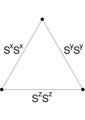
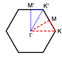
Figure 1: (left) Unit cell of the triangular lattice of model (1) where the Ising-type nearest-neighbor spin couplings on the three non-equivalent bonds – $(\gamma)$-bonds are each perpendicular to the $\gamma\>(=x,\>y,\>z)$ spin quantization axis – have only the $\gamma$-component. (right) First Brillouin zone of the same triangular lattice and principal directions used to represent the spin-wave spectrum: $\Gamma=\left(0,0\right)$, $M=\left(\pi,\pi/\sqrt{3}\right)$, $K=\left(4\pi/3,0\right)$, $M^{\prime}=\left(0,2\pi/\sqrt{3}\right)$, $K^{\prime}=\left(2\pi/3,2\pi/\sqrt{3}\right)$.

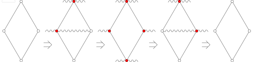
Figure 2: Schematic view of the $4^{th}$ order perturbation process leading to the coupling of the four spins sitting around a diamond, by means of quantum fluctuations [see Eq. (2)]. At each step, spin flips are performed in pairs at one of the diamond four bonds: in the virtual states the location of the misaligned spins are indicated by filled circles and the broken ($z$)-bonds are marked by wavy lines.

2 Model

We consider a spin one-half system (we keep $S$ generic for notational convenience) residing on a triangular lattice lying in the $(1,1,1)$ plane of the spin-quantization frame [see Fig. 1 (left)]. The label $(\gamma)\>(=x,\>y,\>z)$ refers to its three non-equivalent nearest-neighbor bonds spanned by the lattice vectors $\mathbf{a}_{x}=\left(1/2,-\sqrt{3}/2\right)$, $\mathbf{a}_{y}=\left(1/2,\sqrt{3}/2\right)$ and $\mathbf{a}_{z}=\left(1,0\right)$, respectively [see Fig. 1 (left)]. The $(\gamma)$-bond, which is perpendicular to the $\gamma$ spin-quantization axis, hosts nearest-neighbor spin couplings only between the $S_{\mathbf{i}}^{\gamma}$ components of the spin operators $\mathbf{S}_{\mathbf{i}}$ [see Fig. 1(left)], and the corresponding Hamiltonian takes the following form [23]

$$H=-\sum_{\mathbf{i},\gamma}K_{\gamma}S_{\mathbf{i}}^{\gamma}S_{\mathbf{i}+\mathbf{a}_{\gamma}}^{\gamma}\,.$$ (1)

Given that the signs of the $K_{\gamma}$ couplings can be individually flipped by means of a canonical transformation [23], without any loss of generality, we consider hereafter all $K_{\gamma}$ to be positive (ferromagnetic couplings). Then, after the analysis performed in Ref. [23] within the linked-cluster expansion [22], we know that a coupling between pairs of spins belonging to next-nearest-neighbor chains emerges by the quantum corrections induced by the $K_{x}$ and $K_{y}$ terms to the ferromagnetic classical ground state at the $4^{th}$ order in a diamond-shape 4-site cluster (see Fig. 2). The so derived coupling has the following expression

$$\delta H=-K\sum_{\mathbf{i}}\left(S_{\mathbf{i}}^{z}S_{\mathbf{i}+\mathbf{a}_{z}}^{z}\right)S_{\mathbf{i}+\mathbf{a}_{x}}^{z}S_{\mathbf{i}+\mathbf{a}_{y}}^{z}$$ (2)

where $K=\frac{1}{24}\frac{K_{x}^{2}K_{y}^{2}}{\left|K_{z}^{3}\right|}$ and the sites $\mathbf{i}+\mathbf{a}_{x}$ and $\mathbf{\mathbf{i}}+\mathbf{\mathbf{a}}_{y}$ belong to next-nearest-neighbor chains [they are actually the ends of the longer diagonal of the diamond cluster, see Fig. 2]. Given that $S_{\mathbf{i}}^{z}S_{\mathbf{i}+\mathbf{a}_{z}}^{z}$ is just $\frac{1}{4}$ for $K_{z}>0$, the coupling between next-nearest-neighbor chains and the one acting along the chains have the same sign. Taking into account such corrections, we come to the effective Hamiltonian we wish to analyze in this short paper within the linear spin-wave theory:

$$H^{\prime}=H+\delta H.$$ (3)

It is worth noting that, within the linear spin-wave theory, $\delta H$ provides higher-order terms with respect to those emerging from $H$. Accordingly, our treatment of Eq. (3) automatically and exactly avoids any double counting although, obviously, an exact treatment of $H$ will give also the contribution coming from $\delta H$.

3 Spin-wave theory

3.1 Harmonic approximation

First, we apply the linear spin-wave theory to the Hamiltonian (1), i.e. keeping only terms bilinear in the $a$-operators and thus obtaining an $\mathcal{O}\left(1/S\right)$ expansion [23]. In particular, we consider the ferromagnetic state and use the Holstein-Primakoff (HP) transformation

$$S_{\mathbf{i}}^{z}=S-a_{\mathbf{i}}^{\dagger}a_{\mathbf{i}}$$ (4)

$$S_{\mathbf{i}}^{x}=\sqrt{\dfrac{S}{2}}\left(a_{\mathbf{i}}+a_{\mathbf{i}}^{\dagger}\right)$$ (5)

$$S_{\mathbf{i}}^{y}=\dfrac{1}{i}\sqrt{\dfrac{S}{2}}\left(a_{\mathbf{i}}-a_{\mathbf{i}}^{\dagger}\right)$$ (6)

where the bosonic $a_{\mathbf{i}}$ operators, sited at the site $\mathbf{i}$ of the lattice, satisfy canonical commutation relations $\left[a_{\mathbf{i}},a_{\mathbf{j}}^{\dagger}\right]=\delta_{\mathbf{ij}}$ and $\left[a_{\mathbf{i}},a_{\mathbf{j}}\right]=\left[a_{\mathbf{i}}^{\dagger},a_{\mathbf{j}}^{\dagger}\right]=0$. In this representation, the Hamiltonian (1) reads as

$$H =-K_{x}\dfrac{S}{2}\sum_{\mathbf{i}}\left(a_{\mathbf{i}}^{\dagger}a_{\mathbf{i}+\mathbf{a}_{x}}+a_{\mathbf{i+}\mathbf{a}_{x}}^{\dagger}a_{\mathbf{i}}+a_{\mathbf{i}}^{\dagger}a_{\mathbf{i+}\mathbf{a}_{x}}^{\dagger}+a_{\mathbf{i}}a_{\mathbf{i}+\mathbf{a}_{x}}\right)$$

$$-K_{y}\dfrac{S}{2}\sum_{\mathbf{i}}\left(a_{\mathbf{i}}^{\dagger}a_{\mathbf{i}+\mathbf{a}_{y}}+a_{\mathbf{i+}\mathbf{a}_{y}}^{\dagger}a_{\mathbf{i}}-a_{\mathbf{i}}^{\dagger}a_{\mathbf{i+}\mathbf{a}_{y}}^{\dagger}-a_{\mathbf{i}}a_{\mathbf{i}+\mathbf{a}_{y}}\right)$$

$$-NK_{z}S^{2}+K_{z}S\sum_{\mathbf{i}}\left(a_{\mathbf{i}}^{\dagger}a_{\mathbf{i}}+a_{\mathbf{i+}\mathbf{a}_{z}}^{\dagger}a_{\mathbf{i}+\mathbf{a}_{z}}\right)$$ (7)

where $N$ is the number of the lattice sites. Then, using the Fourier transform $a_{\mathbf{i}}=\dfrac{1}{\sqrt{N}}\sum_{\mathbf{k}}e^{i\mathbf{k}\cdot\mathbf{r_{i}}}a_{\mathbf{k}}$ and, therefore, moving to the momentum space, we find

$$H=-NK_{z}S^{2}+\sum_{\mathbf{k}}\left[A_{0}\left(\mathbf{k}\right)a_{\mathbf{k}}^{\dagger}a_{\mathbf{k}}-\dfrac{1}{2}B_{0}\left(\mathbf{k}\right)\left(a_{\mathbf{k}}^{\dagger}a_{-\mathbf{k}}^{\dagger}+a_{\mathbf{k}}a_{-\mathbf{k}}\right)\right],$$ (8)

where $A_{0}\left(\mathbf{k}\right)=S\left(2K_{z}-K_{x}\cos\mathbf{k}_{\mathbf{a}_{x}}-K_{y}\cos\mathbf{k}_{\mathbf{a}_{y}}\right)$, $B_{0}\left(\mathbf{k}\right)=S\left(K_{x}\cos\mathbf{k}_{\mathbf{a}_{x}}-K_{y}\cos\mathbf{k}_{\mathbf{a}_{y}}\right)$, $\mathbf{k}_{\mathbf{a}_{x}}=\mathbf{k}\cdot\mathbf{a}_{x}$ and $\mathbf{k}_{\mathbf{a}_{y}}=\mathbf{k}\cdot\mathbf{a}_{y}$. Accordingly, the magnonic spectrum $\omega\left(\mathbf{k}\right)$ is given by

$$\omega\left(\mathbf{k}\right) =\sqrt{A_{0}^{2}\left(\mathbf{k}\right)-B_{0}^{2}\left(\mathbf{k}\right)}=2S\sqrt{\left(K_{z}-K_{x}\cos\mathbf{k}_{\mathbf{a}_{x}}\right)\left(K_{z}-K_{y}\cos\mathbf{k}_{\mathbf{a}_{y}}\right)}.$$ (9)

It is worth reminding that the ferromagnetic state results the lowest-energy one once introducing the quantum corrections on top of the classical ground state [23].

3.2 Magnon interactions

Then, we intend to see how the spin-wave dispersion is modified upon introducing the higher-order term $\delta H$ (2), leading to the effective Hamiltonian $H^{\prime}$. To this aim, we apply the linear spin-wave theory to this latter (3) and consider again the ferromagnetic state. Keeping only terms bilinear in the $a$-operators, we obtain the following expression for the higher-order term $\delta H$ in real space

$$\delta H=-NKS^{4}+KS^{3}\sum_{\mathbf{i}}\left(a_{\mathbf{i}+\mathbf{a}_{x}}^{\dagger}a_{\mathbf{i}+\mathbf{a}_{x}}+a_{\mathbf{i}+\mathbf{a}_{y}}^{\dagger}a_{\mathbf{i}+\mathbf{a}_{y}}+a_{\mathbf{i}+\mathbf{a}_{z}}^{\dagger}a_{\mathbf{i}+\mathbf{a}_{z}}+a_{\mathbf{i}}^{\dagger}a_{\mathbf{i}}\right).$$ (10)

Next, we move again to the momentum space by means of the same Fourier transform

$$\delta H =-NKS^{4}+4KS^{3}\sum_{\mathbf{k}}a_{\mathbf{k}}^{\dagger}a_{\mathbf{k}}.$$ (11)

Such an expression for $\delta H$ leads to the following one for $H^{\prime}$:

$$H^{\prime} =-N\left(K_{z}+KS^{2}\right)S^{2}+\sum_{\mathbf{k}}\left[A\left(\mathbf{k}\right)a_{\mathbf{k}}^{\dagger}a_{\mathbf{k}}-\dfrac{1}{2}B\left(\mathbf{k}\right)\left(a_{\mathbf{k}}^{\dagger}a_{\mathbf{-k}}^{\dagger}+a_{\mathbf{k}}a_{-\mathbf{k}}\right)\right]$$ (12)

where $A\left(\mathbf{k}\right)=A_{0}\left(\mathbf{k}\right)+4KS^{3}=S\left(2K_{z}+4KS^{2}-K_{x}\cos\mathbf{k}_{\mathbf{a}_{x}}-K_{y}\cos\mathbf{k}_{\mathbf{a}_{y}}\right)$ and $B\left(\mathbf{k}\right)=B_{0}\left(\mathbf{k}\right)=S\left(K_{x}\cos\mathbf{k}_{\mathbf{a}_{x}}-K_{y}\cos\mathbf{k}_{\mathbf{a}_{y}}\right)$. Accordingly, the new spin-wave dispersion $\omega^{\prime}\left(\mathbf{k}\right)$ is

$$\omega^{\prime}\left(\mathbf{k}\right) =\sqrt{A^{2}\left(\mathbf{k}\right)-B^{2}\left(\mathbf{k}\right)}$$

$$=2S\sqrt{\left(K_{z}+2KS^{2}-K_{x}\cos\mathbf{k}_{\mathbf{a}_{x}}\right)\left(K_{z}+2KS^{2}-K_{y}\cos\mathbf{k}_{\mathbf{a}_{y}}\right)}$$ (13)

Comparing the new dispersion $\omega^{\prime}\left(\mathbf{k}\right)$ to the previous one $\omega\left(\mathbf{k}\right)$, Eq. (9), it is evident that the net effect of the $\delta H$ term in the effective Hamiltonian $H^{\prime}$ is the introduction of a rigid (not momentum dependent) shift of $2KS^{2}$ to the Hamiltonian parameter $K_{z}$. Let us analyze in detail the new dispersion $\omega^{\prime}\left(\mathbf{k}\right)$ in the next section and comment briefly on the effects of such a shift.

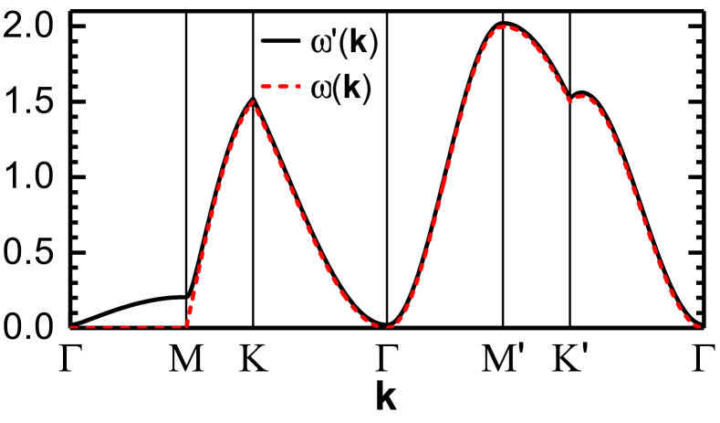
Figure 3: Spin-wave excitation spectra $\omega^{\prime}\left(\mathbf{k}\right)$ and $\omega\left(\mathbf{k}\right)$ for $K_{\gamma}=1$ and $S=1/2$ along the principal directions of the first Brillouin zone ($\Gamma\rightarrow M\rightarrow K\rightarrow\Gamma\rightarrow M^{\prime}\rightarrow K^{\prime}\rightarrow\Gamma$), see dashed red and dotted blue paths in Fig. 1 (right).

4 Results

In Fig. 3, we report the spin-wave excitation spectra $\omega^{\prime}\left(\mathbf{k}\right)$, Eq. (13), and $\omega\left(\mathbf{k}\right)$, Eq. (9), for $K_{\gamma}=1$ and $S=1/2$ along the principal directions of the first Brillouin zone ($\Gamma\rightarrow M\rightarrow K\rightarrow\Gamma\rightarrow M^{\prime}\rightarrow K^{\prime}\rightarrow\Gamma$), see dashed red and dotted blue paths in Fig. 1 (right). As already derived and discussed in Ref. [23], the spin-wave excitation spectrum $\omega\left(\mathbf{k}\right)$ is gapless along the nodal line $\Gamma\rightarrow M$ and all other equivalent-by-symmetry lines in momentum space because of the sub-extensive degeneracy of the classical manifold [23]. Then, it is very remarkable to see that the effective coupling $\delta H$ between pairs of spins belonging to next-nearest-neighbor chains, emerging from a careful treatment of the quantum fluctuations [23], is capable to open up a spin gap along such nodal lines. In particular, for $K_{\gamma}=1$, we have a gap of $\frac{1}{6}S^{3}$ at the bottom of the band (the $\Gamma$ point) and a gap of $\frac{1}{6}S^{3}\sqrt{1+24/S^{2}}$ at the $M$ point. In fact, the previous nodal line $\Gamma\rightarrow M$ acquires a well defined dispersion because of the interplay between the two terms under the square root in Eq. (13): the first of them, $K_{z}+2KS^{2}-K_{x}\cos\mathbf{k}_{\mathbf{a}_{x}}$, is no longer identically zero along $\Gamma\rightarrow M$, and this allows the second one, $K_{z}+2KS^{2}-K_{y}\cos\mathbf{k}_{\mathbf{a}_{y}}$, to provide a dispersion. The rest of the spin-wave excitation spectrum, that is along all other explored lines, is minimally affected as expected. It is worth reminding that $\delta H$ cannot fully lift the degeneracy of the ground state as the two sublattices formed by nearest-neighbor chains remain decoupled because of a hidden symmetry of the model [23].

5 Conclusions

In this short paper, we have analyzed the effects on the spin-wave excitation spectrum of the triangular analog of the Kitaev model [20, 23, 21] of an effective coupling between pairs of spins belonging to next-nearest-neighbor chains emerged by a careful treatment of the quantum fluctuations within the linked-cluster expansion [22] at the $4^{th}$ order [23]: the $K_{x}$ and $K_{y}$ terms induce quantum corrections to the ferromagnetic classical ground state. In absence of such a coupling, the spin-wave excitation spectrum presents nodal lines along the $\Gamma\rightarrow M$ line and all other equivalent-by-symmetry lines in momentum space [23]. It is really remarkable that this effective coupling manages to open up a spin gap in the spectrum, that becomes fully gapped, and induces a well defined dispersion along the $\Gamma\rightarrow M$ line (partially removing the degeneracy in the system), while the rest of the spectrum is minimally affected as expected.

References

- [1] L. Balents, Nature 464 (2010) 199.
- [2] J. Villain, R. Bidaux, J.-P. Carton, R. Conte, J. Phys. France 41 (1980) 1263.
- [3] E. F. Shender, Sov. Phys. JETP 56 (1982) 178.
- [4] L. Savary, K. A. Ross, B. D. Gaulin, J. P. C. Ruff, L. Balents, Phys. Rev. Lett. 109 (2012) 167201.
- [5] G. Jackeli, G. Khaliullin, Phys. Rev. Lett. 102 (2009) 017205.
- [6] A. Kitaev, Annals of Physics 321 (2006) 2.
- [7] J. Chaloupka, G. Jackeli, G. Khaliullin, Phys. Rev. Lett. 105 (2010) 027204.
- [8] H.-C. Jiang, Z.-C. Gu, X.-L. Qi, S. Trebst, Phys. Rev. B 83 (2011) 245104.
- [9] J. Reuther, R. Thomale, S. Trebst, Phys. Rev. B 84 (2011) 100406.
- [10] C. C. Price, N. B. Perkins, Phys. Rev. Lett. 109 (2012) 187201.
- [11] J. Chaloupka, G. Jackeli, G. Khaliullin, Phys. Rev. Lett. 110 (2013) 097204.
- [12] Y. Singh, P. Gegenwart, Phys. Rev. B 82 (2010) 064412.
- [13] X. Liu, T. Berlijn, W.-G. Yin, W. Ku, A. Tsvelik, Y.-J. Kim, H. Gretarsson, Y. Singh, P. Gegenwart, J. P. Hill, Phys. Rev. B 83 (2011) 220403.
- [14] S. K. Choi, R. Coldea, A. N. Kolmogorov, T. Lancaster, I. I. Mazin, S. J. Blundell, P. G. Radaelli, Y. Singh, P. Gegenwart, K. R. Choi, S.-W. Cheong, P. J. Baker, C. Stock, J. Taylor, Phys. Rev. Lett. 108 (2012) 127204.
- [15] Y. Singh, S. Manni, J. Reuther, T. Berlijn, R. Thomale, W. Ku, S. Trebst, P. Gegenwart, Phys. Rev. Lett. 108 (2012) 127203.
- [16] F. Ye, S. Chi, H. Cao, B. C. Chakoumakos, J. A. Fernandez-Baca, R. Custelcean, T. F. Qi, O. B. Korneta, G. Cao, Phys. Rev. B 85 (2012) 180403.
- [17] H. Gretarsson, J. P. Clancy, Y. Singh, P. Gegenwart, J. P. Hill, J. Kim, M. H. Upton, A. H. Said, D. Casa, T. Gog, Y.-J. Kim, Phys. Rev. B 87 (2013) 220407.
- [18] G. Khaliullin, Prog. Theor. Phys. Suppl. 160 (2005) 155.
- [19] I. Rousochatzakis, U. K. Rössler, J. van den Brink, M. Daghofer, Phys. Rev. B 93 (2016) 104417.
- [20] M. Becker, M. Hermanns, B. Bauer, M. Garst, S. Trebst, Phys. Rev. B 91 (2015) 155135.
- [21] K. Li, S.-L. Yu, J.-X. Li, New Journal of Physics 17 (4) (2015) 043032.
- [22] M. P. Gelfand, R. R. P. Singh, Adv. Phys. 49 (2000) 93.
- [23] G. Jackeli, A. Avella, Phys. Rev. B 92 (2015) 184416.