Interpolating vector fields for near identity maps and averaging

Abstract

For a smooth near identity map, we introduce the notion of an interpolating vector field written in terms of iterates of the map. Our construction is based on Lagrangian interpolation and provides an explicit expressions for autonomous vector fields which approximately interpolate the map. We study properties of the interpolating vector fields and explore their applications to the study of dynamics. In particular, we construct adiabatic invariants for symplectic near identity maps. We also introduce the notion of a Poincaré section for a near identity map and use it to visualise dynamics of four dimensional maps. We illustrate our theory with several examples, including the Chirikov standard map and a symplectic map in dimension four, an example motivated by the theory of Arnold diffusion.

1 Introduction

Near identity maps naturally appear in several branches of mathematics and mathematical physics. They are often used for numerical integration of ordinary differential equations and for studying the evolution under fast time-periodic forcing. In the perturbation theory of integrable Hamiltonian systems with three degrees of freedom, near identity maps are used to describe dynamics in a small neighbourhood of a double resonance, see e.g. [6]. The last problem is one of the central topics in the study of the Arnold diffusion. In these problems some important details of the discussion depend on the smoothness class of the map and, for the sake of simplicity, we mainly consider the infinitely differentiable case and, where appropriate, assume analyticity.

It is well known that a near identity map $F_{\epsilon}$, where $|\epsilon|\ll 1$ and $F_{0}=\mathrm{I}$, is formally embedded into an autonomous flow [13]. Indeed, a formal construction can be used to find a vector field in the form of a formal power series in $\epsilon$ such that the formal series of the corresponding time-$\epsilon$ map coincides with the Taylor series of the original map. Truncated series define a vector field which interpolates the map with an error of order of the first omitted term. Note that this construction is formal only as in general the map cannot be embedded into an autonomous flow, i.e. generic $F_{\epsilon}$ cannot be represented as a time-$\epsilon$ map of an autonomous vector field [7]. Nevertheless, the difference between them can be made a flat function in $\epsilon$ at $\epsilon=0$ [11].

An alternative approach to the study of near identity maps is based on averaging (see e.g. [7]). A near identity map $F_{\epsilon}$ can be written as a time-$\epsilon$ map of a time-periodic vector field called a suspension of the map. Then the averaging procedure can be used recursively to eliminate the time-dependence up to any order of the small parameter. In the analytic case, a suspension can be found in the form of an analytic autonomous vector field plus an exponentially small non-autonomous term [7] (see also [2] for a concrete example).

Both these methods are constructive, nevertheless, none of them provides an easy way to find an explicit expression for a vector field which approximately interpolates the map. In this paper we propose a new method for construction of such vector fields with the help of the Lagrange interpolation of iterates of the map, henceforth referred to as interpolating vector fields. We analyse the errors of the approximation of $F_{\epsilon}$ by the time-$\epsilon$ map of the interpolating vector fields.

The interpolating vector fields provide a useful tool for analysis of dynamics. In particular, we introduce the notion of a “Poincaré section” for the map $F_{\epsilon}$. Similarly to classical Poincaré section, this construction reduces the dimension of the phase space by one and, consequently, can be used to visualise trajectories of four-dimensional maps. Compared to the method of phase-space slices traditionally used for this purpose (see e.g. [9]) our method apparently shows higher resolution of details.

In the case when the map $F_{\epsilon}$ is symplectic, an interpolating vector field can be used to construct an adiabatic invariant $h_{n}$ where $n$ stands for the order of the interpolating vector field. The function $h_{n}$ is approximately preserved for many iterates of the map and can be used for a further reduction of the dimension.

In order to illustrate the effectiveness of the method and before discussing technical details involved in the construction, let us consider a 4-dimensional near identity Froeschlé-like symplectic diffeomorphism $T_{\epsilon}$ defined on $\mathbb{T}^{2}\times\mathbb{R}^{2}$. In coordinates $(\psi_{1},\psi_{2},J_{1},J_{2})$ this map is defined by the equation (3.5) but the precise expression is not important for the current discussion. Let $\Sigma$ be a three-dimensional cylinder defined by the equality $\psi_{1}=\psi_{2}$. Fig. 1(a) shows points from several trajectories of $T_{\epsilon}$ projected along an interpolating vector field onto $\Sigma$. We call this picture a Poincaré section for the map $T_{\epsilon}$.

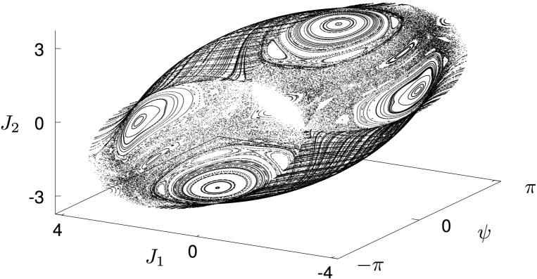
(a)

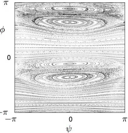
(b)(c)

Figure 1: Dynamics of a symplectic map on a four-dimensional cylinder $\mathbb{T}^{2}\times\mathbb{R}^{2}$. The map is defined by (3.5) with parameter given by (3.6), $\epsilon=0.35$, and 400 initial conditions are taken on $\Sigma\cap\{h_{10}=4\}$ (see Section 3 for details of the model and numerical techniques used to produce these pictures). (a) Trajectories of the map are projected on a three-dimensional Poincaré section (a three dimensional cylinder $\mathbb{T}\times\mathbb{R}^{2}$) along an interpolating vector field. Note that all points are in a small neighbourhood of a two-dimensional torus. (b) A two dimensional projection of (a) using the coordinate $\phi=\arg(J_{1}+iJ_{2})\in(-\pi,\pi]$ for the vertical axis. The analogy with the phase space of a two-dimensional area-preserving map is apparent. (c) A magnification of (b) where further details can be observed.

In Fig. 1 all initial conditions are chosen from a torus defined by the intersection of $\Sigma$ with a level set of the adiabatic invariant $h_{10}$. Since $h_{10}$ is approximately preserved by the map, all points shown on Fig. 1(a) are in a small neighbourhood of the torus. Then a clearer image of the dynamics is obtained with the help two angular coordinates, namely, $\psi$ and $\phi=\arg(J_{1}+iJ_{2})$. Fig. 1(b) shows the projection of Fig. 1(a) onto the torus $(\psi_{1},\phi)$, and Fig. 1(c) is a magnification of a strip located near the top of Fig. 1(b). These picture reveal that the four-dimensional dynamics of $T_{\epsilon}$ resemble a two-dimensional area-preserving map. This similarity can be explained with the help of the normal form theory [8]. The latter also provides an alternative visualisation method (see [4]). We stress that the method of this paper is much easier to implement and provides higher accuracy in representation of details of the dynamics as our pictures represent true trajectories of $T_{\epsilon}$ since the interpolation is used only for selecting initial conditions and projecting points onto $\Sigma$. The details of the model and the method are described in Section 3.

To give more formal definitions for the objects discussed in this paper, consider a smooth one-parameter near identity family of maps $F_{\epsilon}:D\to\mathbb{R}^{m}$ where $m\geq 1$, $D\subset\mathbb{R}^{m}$ is an open domain and $|\epsilon|<\epsilon_{0}$. Then the map can be written in the form

$$F_{\epsilon}(x)=x+\epsilon\,G_{\epsilon}(x).$$

The function $G_{0}$ obtained by setting $\epsilon=0$ is often called a limit vector field. Its time-$\epsilon$ map is $\epsilon^{2}$-close to $F_{\epsilon}$.

The central object of this paper is an interpolating vector field for the near identity map $F_{\epsilon}$ defined in the following way. Fix a positive integer $n$. Let $x\in D$ and suppose that the iterates $x_{k}=F_{\epsilon}^{k}(x)\in D$ are defined for $-n\leq k\leq n$. Then there is a unique polynomial $p_{n}$ of degree $2n$ in $t$ such that

$$x_{k}=p_{n}(t_{k},x_{0},\epsilon)$$ (1.1)

for every $t_{k}=\epsilon k$ with $|k|\leq n$. The coefficients of $p_{n}$ depend on $x$ and $\epsilon$. The interpolating vector field is defined as the velocity vector of the interpolating curve at $t=0$, i.e.,

$$X_{n}(x,\epsilon)=\partial_{t}p_{n}(0,x,\epsilon)$$ (1.2)

where $\partial_{t}p_{n}$ denotes the derivative of $p_{n}$ with respect to $t$. In Section 2 we will use the Lagrange interpolation to show that the interpolating vector field $X_{n}$ is a linear combination of the iterates of the initial point $x=x_{0}$,

$$X_{n}(x,\epsilon)=\epsilon^{-1}\sum_{k=1}^{n}p_{nk}\left(x_{k}-x_{-k}\right),$$ (1.3)

where

$$p_{nk}=\frac{(-1)^{k+1}(n!)^{2}}{k(n+k)!(n-k)!}\,.$$ (1.4)

Note that the coefficients $p_{nk}$ are independent of the map $F_{\epsilon}$, e.g., for $n=1$ we get

$$X_{1}(x,\epsilon)=\frac{F_{\epsilon}(x)-F_{\epsilon}^{-1}(x)}{2\epsilon}.$$

We will show that the time-$\epsilon$ map of this vector field is $|\epsilon|^{3}$-close to $F_{\epsilon}$. Thus $X_{1}$ can provide a more accurate interpolation for $F_{\epsilon}$ than the limit flow.

If $F_{\epsilon}:D\to D$ is a diffeomorphism, then the domain $D$ is invariant and the equation (1.3) defines $X_{n}$ on $D$ for every $n\in\mathbb{N}$. In general, we do not assume that $D$ is invariant, and iterates of a point $x_{0}\in D$ may leave the domain. Nevertheless, it is not difficult to show that for any compact subset $D_{0}\subset D$, there is a constant $r_{0}>0$ such that $x_{k}=F_{\epsilon}^{k}(x)$ is defined for every $x\in D_{0}$ and every integer $k$ provided $|\epsilon k|\leq r_{0}$. Therefore $X_{n}$ is defined on $D_{0}$ for every $n\leq r_{0}|\epsilon|^{-1}$.

If the map $F_{\epsilon}$ is a lift of a diffeomorphism of a torus or cylinder, then the interpolating vector field is also a lift of a vector field defined on the same manifold. It is possible to generalize the definition onto a general manifold but this discussion is beyond the aims of the present paper.

We note that if $F_{\epsilon}$ and $F_{\epsilon}^{-1}$ are both polynomial (e.g. the classical Hénon map and its generalisations), then the interpolating vector field is also polynomial.

In the symplectic case, the interpolating vector fields remove the need of computing an averaged Hamiltonian. This opens an opportunity of performing massive numerical explorations of a multi-dimensional phase space, reducing the computation time significantly. Possible dynamical applications of this visualizing techniques include, among others, studying of area-preserving maps in $\mathbb{C}^{2}$ and of Arnold diffusion for 4-dimensional symplectic maps near double resonances.

The rest of this paper is organised as follows. In Section 2 we briefly summarise the Lagrangian interpolation theory and derive some properties of the interpolating vector fields. Then we analyse the accuracy of interpolation. We discuss connections between the interpolating vector field and suspensions of the map $F_{\epsilon}$. In particular, we discuss connections to averaging methods and the optimality of choosing $n$ as a function of $\epsilon$. We show that in the analytic case the interpolation error can become exponentially small in $\epsilon$. Finally, in subsection 2.5 we consider the symplectic setting. Although the interpolating vector field $X_{n}$ is not symplectic, it still can be used to define an adiabatic invariant $h_{n}$ which remains approximately constant for about $\epsilon^{-2n}$ iterates of the map $F_{\epsilon}$.

In Section 3 we present results of our numerical experiments to illustrate the use of the interpolating vector fields for exploring the dynamics of maps in regions where they are near the identity. First, in Section 3.1 we consider the 2-dimensional symplectic case and perform experiments with the Chirikov standard map as a model. This is a preliminary example which illustrates various useful features of the interpolating vector fields. Moreover, one can compare the interpolating vector field directly with the map as the two dimensional dynamics is easy to visualize.

The main advantage of interpolating vector fields is that they provide a useful tool to investigate higher dimensional phase spaces. In particular, they provide a powerful tool for computing projections of the discrete dynamics onto subspaces of codimension-one. We use this tool to define Poincaré sections for maps, an extension of the classical construction traditionally restricted to systems with continuous time only, see details in Section 3.2. We illustrate this construction for the 4-dimensional symplectic map $T_{\epsilon}$ to obtain representations of different types of its dynamics with the help of plots in dimensions two and three.

2 Interpolating vector fields

2.1 Lagrange interpolating polynomials

An interpolating polynomial can be explicitly written with the help of Lagrange interpolating polynomials (see e.g. [12]). Suppose that nodes are located at integer points symmetrically with respect to $\tau=0$. Then Lagrange’s fundamental interpolating polynomial is

$$\pi_{n}(\tau)=\prod_{k=-n}^{n}(\tau-k)$$ (2.1)

and Lagrange’s basis polynomials are

$$\pi_{nk}(\tau)=\frac{\pi_{n}(\tau)}{\pi_{n}^{\prime}(k)(\tau-k)}.$$ (2.2)

For every $n\in\mathbb{N}$ and $|k|\leq n$ the equation (2.2) defines the unique polynomial of degree $2n$ such that $\pi_{nk}(j)=\delta_{kj}$ for every $|j|\leq n$, where $\delta_{kj}$ is the Kronecker delta. For $1\leq|k|\leq n$ we differentiate the equation (2.2) and, taking into account that $\pi_{n}(0)=0$, we get $\pi_{nk}^{\prime}(0)=-\frac{\pi_{n}^{\prime}(0)}{k\pi_{n}^{\prime}(k)}.$ Since $\pi_{n}^{\prime}(0)=(-1)^{n}(n!)^{2}$ and

$$\pi_{n}^{\prime}(k)=\prod_{j=-n}^{k-1}(k-j)\prod^{n}_{j=k+1}(k-j)=(-1)^{n-k}(n+k)!(n-k)!$$ (2.3)

we conclude that $\pi_{nk}^{\prime}(0)=p_{nk}$ where

$$p_{nk}=\frac{(-1)^{k+1}(n!)^{2}}{k(n+k)!(n-k)!}\,.$$ (2.4)

Since $\pi_{n}$ is odd, $\pi_{n0}$ is even and, consequently, $p_{n0}=\pi_{n0}^{\prime}(0)=0$. The constants $p_{nk}$ are used in the equation (1.3) which defines the interpolating vector fields. Later we will need some properties of these constants.

Proposition 2.1.

For every $n$ fixed, $(-1)^{k+1}p_{nk}$ is a monotone decreasing positive sequence for $1\leq k\leq n$, and $p_{n,{-}k}=-p_{nk}$. Moreover,

$$\sum_{k=-n}^{n}p_{nk}k^{j}=\begin{cases}1,&\mbox{if $j=1$},\\ 0,&\mbox{if $j=0$ or $2\leq j\leq 2n$},\end{cases}$$ (2.5)

$$\sum_{k=1}^{n}|p_{nk}|=\frac{H_{n}}{2}\qquad\mbox{and}\qquad\sum_{k=1}^{n}p_{nk}=H_{2n}-H_{n},$$ (2.6)

where $H_{n}=\sum_{k=1}^{n}k^{-1}$ is the $n$-th harmonic number.

Proof.

The first equality can be derived from the following observation. Let $0\leq j\leq 2n$. Interpolating any polynomial of degree $j$ with the help of a polynomial of degree $2n$, we recover the original polynomial. Applying this rule to $\tau^{j}$ we get that

$$\sum_{k=-n}^{n}\pi_{nk}(\tau)k^{j}=\tau^{j}.$$

Differentiating this equality with respect to $\tau$ at $\tau=0$ we obtain (2.5). ∎

Let $r>0$ and consider a continuous curve $\gamma:[-r,r]\to\mathbb{R}^{m}$. For any $\epsilon\neq 0$ and $n\in\mathbb{N}$ such that $n|\epsilon|<r$, the equation

$$p_{n}(t,\epsilon)=\sum_{k=-n}^{n}\pi_{nk}(\epsilon^{-1}t)\gamma(k\epsilon)$$

defines the unique polynomial of degree $2n$ such that $p_{n}(k\epsilon,\epsilon)=\gamma(k\epsilon)$ for $|k|\leq n$. Let $v_{n}(\gamma,\epsilon)=\partial_{t}p_{n}(0,\epsilon)$. Taking into account the expression for $p_{n}$ we get

$$v_{n}(\gamma,\epsilon)=\epsilon^{-1}\sum_{k=-n}^{n}p_{nk}\gamma(k\epsilon).$$ (2.7)

Note that although this definition contains a division by $\epsilon$, the following lemma implies that $v_{n}$ can be extended to $\epsilon=0$ by continuity provided the curve is sufficiently smooth.

Lemma 2.2.

If $\gamma\in\mathcal{C}^{2n+1}\bigl{(}[-r,r]\bigr{)}$ and $|\epsilon|n<r$, then

$$\left|\dot{\gamma}(0)-v_{n}(\gamma,\epsilon)\right|\leq\frac{\epsilon^{2n}(n!)^{2}}{(2n+1)!}\max_{|t|\leq r}\left|\gamma^{(2n+1)}(t)\right|.$$ (2.8)

Proof.

The standard theory of interpolating polynomials, see e.g. [12], states that

$$\gamma(t)=p_{n}(t,\epsilon)+\frac{\epsilon^{2n+1}\pi_{n}(\epsilon^{-1}t)}{(2n+1)!}w_{n}(t,\epsilon),$$

where the function $w_{n}$ can be expressed as $w_{n}(t,\epsilon)=\gamma^{(2n+1)}(\tau_{*}(t,\epsilon))$ with $\tau_{*}(t,\epsilon)\in[-n\epsilon,n\epsilon]$, an intermediate value of the time variable. Since the zeroes of $\pi$ are all simple, $w$ is continuous at $t=k\epsilon$. Differentiating with respect to $t$ at $t=0$ and taking into account that $\pi_{n}(0)=0$, we get

$$\dot{\gamma}(0)=v_{n}(\gamma,\epsilon)+\frac{\epsilon^{2n}\pi_{n}^{\prime}(0)}{(2n+1)!}\gamma^{(2n+1)}(\tau_{*}(0,\epsilon)).$$

The estimate of the lemma immediately follows from (2.3). This inequality implies that $v_{n}(\gamma,\epsilon)\to\dot{\gamma}(0)$ when $\epsilon\to 0$. ∎

Lemma 2.3 (stability with respect to perturbations).

If $\gamma_{1},\gamma_{2}\in\mathcal{C}^{0}([-r,r])$, $\epsilon\neq 0$ and $n|\epsilon|<r$, then

$$\left|v_{n}(\gamma_{2},\epsilon)-v_{n}(\gamma_{1},\epsilon)\right|\leq|\epsilon|^{-1}H_{n}\left\|\gamma_{2}-\gamma_{1}\right\|$$

where $H_{n}=\sum_{k=1}^{n}k^{-1}$ is the $n$-th harmonic number.

Proof.

Using (2.7) and the triangle inequality we get

$$\left|v_{n}(\gamma_{2},\epsilon)-v_{n}(\gamma_{1},\epsilon)\right| \leq |\epsilon|^{-1}\sum_{k=-n}^{n}|p_{nk}|\left|\gamma_{2}(k\epsilon)-\gamma_{1}(k\epsilon))\right|$$

$$\leq |\epsilon|^{-1}\left\|\gamma_{2}-\gamma_{1}\right\|\sum_{k=-n}^{n}|p_{nk}|.$$

Then the first equality in (2.6) implies the estimate of the lemma. ∎

2.2 Basic properties of interpolating vector fields

The interpolating polynomial of the equation (1.1) can be explicitly written in the form of a Lagrange interpolating polynomial, namely,

$$p_{n}(t,x,\epsilon)=\sum_{k=-n}^{n}\pi_{nk}(\epsilon^{-1}t)x_{k},\quad\text{ where }x_{k}=F_{\epsilon}^{k}(x).$$

Differentiating this equality with respect to $t$ at $t=0$ and using that $\pi_{nk}^{\prime}(0)=p_{nk}$, we recover the explicit expression (1.3) for the interpolating vector field (1.2):

$$X_{n}(x,\epsilon)=\epsilon^{-1}\sum_{k=-n}^{n}p_{nk}x_{k}=\epsilon^{-1}\sum_{k=1}^{n}p_{nk}(x_{k}-x_{-k}).$$ (2.9)

For example, for $n=2$ we get

$$X_{2}(x,\epsilon)=\frac{2}{3\epsilon}\left(F_{\epsilon}(x)-F_{\epsilon}^{-1}(x)\right)-\frac{1}{12\epsilon}\left(F_{\epsilon}^{2}(x)-F_{\epsilon}^{-2}(x)\right).$$

The definition of the interpolating vector field involves division by $\epsilon$, but we will see that $X_{n}$ can be continuously extended to $\epsilon=0$.

Proposition 2.4.

Let $D_{0}\subset D$ be compact. Then there is $r_{0}>0$ such that the interpolating vector field is defined for all $x\in D_{0}$ and all $n\in\mathbb{N}$ such that $n|\epsilon|\leq r_{0}$. For every $n$, the interpolating vector field $X_{n}$ is as smooth as the map $F_{\epsilon}$ itself and $X_{n}(x,0)=G_{0}(x).$

Proof.

Let $F_{\epsilon}(x)=x+\epsilon G_{\epsilon}(x)=x+\epsilon g_{1}(x,\epsilon)$. Obviously, $g_{1}(x,0)=G_{0}(x)$. Then the finite induction implies that

$$x_{k}=F_{\epsilon}^{k}(x)=x_{0}+\epsilon\sum_{j=0}^{k-1}g_{1}(x_{j},\epsilon)$$ (2.10)

for every $k\in\mathbb{N}$ such that $x_{j}\in D$ for all $0\leq j\leq k$. Similarly, the inverse function theorem implies that $F^{-1}_{\epsilon}(x)=x-\epsilon g_{-1}(x,\epsilon)$, where $g_{-1}(x,0)=-G_{0}(x)$. Repeating the previous arguments we conclude that

$$x_{-k}=F_{\epsilon}^{-k}=x_{0}+\epsilon\sum_{j=0}^{k-1}g_{-1}(x_{-j},\epsilon).$$ (2.11)

Using the finite induction, the equations (2.10) and (2.11) and compactness of $D_{0}$, we prove that there is $r_{0}>0$ such that $F^{k}_{\epsilon}(x)\in D$ for all $x\in D_{0}$ provided $|k\epsilon|<r_{0}$.

Substituting the expressions (2.10) and (2.11) into the definition (2.9) of $X_{n}$, and using (2.5) with $j=0$, we obtain

$$X_{n}(x,\epsilon)=\sum_{k=-n}^{n}p_{nk}\sum_{j=0}^{|k|-1}g_{\mathrm{sign}(k)}(x_{\mathrm{sign}(k)j},\epsilon)$$ (2.12)

and the smoothness of $X_{n}$ follows directly. Finally, we note that if $\epsilon=0$, then $x_{j}=x_{0}=x$ for every $j$. Substituting $\epsilon=0$ into the equation (2.12) we get

$$X_{n}(x,0)=\sum_{k=-n}^{n}p_{nk}\sum_{j=0}^{|k|-1}g_{\mathrm{sign}(k)}(x,0)=\sum_{k=-n}^{n}p_{nk}kG_{0}(x).$$

Then the equation (2.5) with $j=1$ implies that $X_{n}(x,0)=G_{0}(X)$. ∎

An interpolating vector field can be used to approximately restore a vector field from its time-$\epsilon$ map.

Proposition 2.5.

Let $\Phi^{\tau}$ be a time-$\tau$ flow of a smooth autonomous vector field $Y$ and $n\in\mathbb{N}$. Let $X_{n}$ be an interpolating vector field for the map $\Phi^{\epsilon}$. Then

$$Y(x)=X_{n}(x,\epsilon)+O(\epsilon^{2n}).$$

The estimate is uniform on every compact subset of $D$.

Proof.

Let $x\in D$ and $\gamma$ be a solution of the initial value problem for the ordinary differential equation $\dot{\gamma}=Y(\gamma)$, $\gamma(0)=x$. Then Proposition 2.5 follows from Lemma 2.2 as the solution is smooth. ∎

We note that the following arguments can also be used to prove the proposition. Expanding the solution $\gamma$ of the initial value problem into Taylor series in time we get

$$\gamma(t)=x+\sum_{k=1}^{2n}\frac{t^{k}}{k!}\gamma^{(k)}(0)+r_{2n}(t)$$

where $\gamma^{(1)}(0)=Y(x)$ and $r_{2n}(t)=O(t^{2n+1})$. Substituting this expression into the definition of the interpolating vector field we get

$$\epsilon X_{n}(x,\epsilon) = \sum_{k=-n}^{n}p_{nk}\gamma(\epsilon k)=\sum_{k=-n}^{n}p_{nk}\left(\sum_{j=1}^{2n}\frac{\epsilon^{j}k^{j}}{j!}\gamma^{(j)}(0)+r_{2n}(k\epsilon)\right)$$

$$= \sum_{j=1}^{2n}\frac{\epsilon^{j}}{j!}\gamma^{(j)}(0)\sum_{k=-n}^{n}k^{j}p_{nk}+R_{n}(\epsilon)=\epsilon Y(x)+R_{n}(\epsilon),$$

where $R_{n}(\epsilon)=\sum_{k=-n}^{n}p_{nk}r_{2n}(k\epsilon)=O(|\epsilon|^{2n+1})$. Here we used the equation (2.5) to simplify the sum.

Remark 2.6.

If $x_{0}$ is a fixed point of $F_{\epsilon}$, then $x_{0}$ is an equilibrium of $X_{n}$.

Remark 2.7.

For a fixed $n$ and a small $\epsilon$ the interpolating vector field $X_{n}(x,\epsilon)$ only involves values of $F_{\epsilon}$ from a small neighbourhood of the point $x$.

Remark 2.8.

If $F_{\epsilon}$ is a lift of a map defined on a cylinder (or a torus), then the interpolating vector field $X_{n}$ is also a lift of a vector field defined on the same manifold. This argument also applies to every manifold obtained by factorising $\mathbb{R}^{m}$ with respect to action of a discrete group of (affine) linear transformations.

We recall that a map $F_{\epsilon}$ is called reversible, if there is an involution $R$ (i.e., $R\circ R=\mathrm{I}$) which conjugates the map and its inverse, i.e., $F_{\epsilon}^{-1}=R\circ F_{\epsilon}\circ R$. The involution $R$ is called a reversor. In this paper we consider only the case when $R$ is a linear map. This case is often used in applications.

Proposition 2.9.

If $F_{\epsilon}$ is a reversible map with a linear reversor $R$, then the interpolating vector field is also reversible, i.e. the application of the map $R$ changes the direction of time:

$$X_{n}(Rx)=-RX_{n}(x).$$

This proposition is proved by a straightforward computation using the symmetric expression for the interpolating vector field (1.3) and the fact that the reversor $R$ maps a trajectory of $F_{\epsilon}$ into a trajectory of $F_{\epsilon}^{-1}$.

Let $F_{\epsilon}$ be a map defined on an one-dimensional interval. Suppose that $x_{0}\in\mathbb{R}$ is a fixed point of $F_{\epsilon}$ and let $\lambda_{\epsilon}=F^{\prime}_{\epsilon}(x_{0})$. Then $x_{0}$ is an equilibrium for the interpolating vector field, i.e. $X_{n}(x_{0})=0$, and

$$X_{n}^{\prime}(x_{0})=\epsilon^{-1}\sum_{k=1}^{n}p_{nk}\left(\lambda_{\epsilon}^{k}-\lambda_{\epsilon}^{-k}\right).$$

If $\epsilon$ is sufficiently small, the linear stability type of the fixed point is the same for the map and for the interpolating vector field. Moreover, since $F_{\epsilon}$ is a monotone function, it is easy to see that the time-$\epsilon$ map of the interpolating vector field is topologically conjugate to $F_{\epsilon}$. On the other hand, in general, the conjugating function cannot be differentiable as the multipliers $\lambda_{\epsilon}$ and $\exp(\epsilon X_{n}^{\prime}(x_{0}))$ of the fixed points can be different. The conclusions about topological equivalence do not require hyperbolicity of $F_{\epsilon}$ and do not generalize to higher dimensions.

2.3 Suspensions of a map and averaging

In general it is not possible to construct an autonomous vector field such that its time-$\epsilon$ map coincides with $F_{\epsilon}$. On the other hand, it is possible to construct a time-periodic vector field with this property. Such vector field is called a suspension of $F_{\epsilon}$. Suppose that $Y$ is a suspension of $F_{\epsilon}$. This vector field has the following characteristic property: if $\xi=\xi(\tau,x,\epsilon)$ is a solution of the initial value problem

$$\partial_{\tau}\xi=\epsilon Y(\tau,\xi,\epsilon),\qquad\xi(0,x,\epsilon)=x\,,$$ (2.13)

then $\xi(1,x,\epsilon)=F_{\epsilon}(x)$. Note that we use the fast time $\tau=\epsilon^{-1}t$ instead of the slow time $t$.

It is not too difficult to construct a suspension. Indeed, let $\chi:[0,1]\to[0,1]$ be a monotone smooth ($\mathcal{C}^{\infty}$) function, such that $\chi(0)=0$, $\chi(1)=1$ and $\chi^{(k)}(0)=\chi^{(k)}(1)=0$ for all $k\in\mathbb{N}$. Then consider a curve parametrized by the function

$$\xi(\tau,x,\epsilon)=x+\epsilon\chi(\tau)G_{\epsilon}(x)$$ (2.14)

with $\tau\in[0,1]$. This curve connects the points $x$ and $F_{\epsilon}(x)=x+\epsilon G_{\epsilon}(x)$. Consider the map $\Phi_{\epsilon}^{\tau}:x\mapsto\xi(\tau,x,\epsilon)$. This map is $\epsilon$-close to the identity in the $\mathcal{C}^{1}$ topology and, hence, a local diffeomorphism by the inverse function theorem. Let $\Psi_{\epsilon}^{\tau}=\left(\Phi_{\epsilon}^{\tau}\right)^{-1}$ and consider a non-autonomous vector field

$$Y(\tau,x,\epsilon)=\chi^{\prime}(\tau)G_{\epsilon}(\Psi_{\epsilon}^{\tau}(x))$$ (2.15)

originally defined for $\tau\in[0,1]$ and extended periodically as a function of $\tau$. It is easy to see that $Y$ is smooth.

Obviously, the function (2.14) is a solution of the initial value problem (2.13) with the vector-field defined by (2.15). Consequently, the time-$\tau$ map of the vector field $\epsilon Y$ coincides with $\Phi^{\tau}_{\epsilon}$ for $\tau\in[0,1]$. Since $\Phi_{\epsilon}^{1}=F_{\epsilon}$, the vector field $Y$ is a suspension of the map $F_{\epsilon}$.

Note that in this construction solutions of the differential equations (2.13) are given explicitly for $\tau\in[0,1]$. These solutions extend recursively to other values of $\tau$ using the identity $\xi(\tau,x,\epsilon)=\xi(\tau-1,F_{\epsilon}(x),\epsilon)$. Since the function $\chi$ is flat at $\tau=0$ and $\tau=1$, the function $\xi$ is smooth in time as long as the solution remains in $D$. It is also possible to use the flow $\Phi^{\tau}_{\epsilon}(x)=F_{\epsilon\chi(\tau)}(x)$ instead of (2.14) in the construction of the suspension.

A suspension of $F_{\epsilon}$ is not unique and we are interested in finding a suspension which is as close to an autonomous vector field as possible. This task can be performed with the help of averaging [1]. An averaging step consists of a substitution of the form

$$\xi=\xi_{1}+S(\tau,\xi_{1},\epsilon)$$ (2.16)

where the function $S$ is periodic in $\tau$. Substituting (2.16) into the differential equation (2.13) we get

$$(1+\partial_{\xi}S)\partial_{\tau}\xi_{1}+\partial_{\tau}S=\epsilon Y(\tau,\xi_{1}+S,\epsilon)$$ (2.17)

where $S$ is evaluated at $(\tau,\xi_{1},\epsilon)$. Let $\langle Y\rangle=\int_{0}^{1}Yd\tau$ be the mean value of $Y$ over its period in $\tau$, and $\tilde{Y}=Y-\langle Y\rangle$ be its oscillatory part with zero mean. It is convenient to let

$$S(\tau,\xi,\epsilon)=\epsilon\int_{0}^{\tau}\tilde{Y}(t,\xi,\epsilon)\,dt.$$

This function is periodic in $\tau$ and $S(k,\xi,\epsilon)=0$ for every $k\in\mathbb{Z}$. Then the map $\xi_{1}\mapsto\xi$ is $\epsilon$-close to the identity for every $\tau$ and is exactly the identity for $\tau\in\mathbb{Z}$. Therefore, the change of variables (2.16) transforms $Y$ into another suspension of the same map $F_{\epsilon}$. Multiplying the equation (2.17) by the matrix $(1+\partial_{\xi}S)^{-1}$, we write the new suspension in the form

$$\partial_{\tau}\xi_{1}=\epsilon Y_{1}(\tau,\xi_{1},\epsilon),$$

where

$$Y_{1}(\tau,\xi_{1},\epsilon)=(1+\partial_{\xi}S)^{-1}\bigl{(}Y(\tau,\xi_{1}+S,\epsilon)-\tilde{Y}(\tau,\xi_{1},\epsilon)\bigr{)}.$$

Taking into account that $S=O(|\epsilon|)$, the definition of $\tilde{Y}$ and differentiability of $Y$ and $S$, we can check that the oscillatory part of $Y_{1}$ vanishes at the leading order, i.e., $\|\tilde{Y}_{1}\|=O(\|\epsilon\tilde{Y}\|)$. The averaging procedure can be repeated to further decrease the time-dependent part of the suspension. Note that the expression for the vector field $Y_{1}$ contains a first derivative with respect to the space variable, thus if $Y\in\mathcal{C}^{k}$ then we can claim that $Y_{1}\in\mathcal{C}^{k-1}$ only and the maximum number of averaging steps is bounded by the smoothness class of $Y$. If $Y$ is infinitely differentiable, the time-dependent part of the suspension vector field can be made smaller than any power of $|\epsilon|$ by repeating the averaging procedure multiple times: after $n$ steps we obtain a suspension of the form

$$Y_{n}(\tau,x,\epsilon)=A_{n}(x,\epsilon)+\epsilon^{n}B_{n}(\tau,x,\epsilon).$$ (2.18)

Neishtadt [7] proved that if $Y$ is analytic in a complex neighbourhood of $D$ then after $n\sim|\epsilon|^{-1}$ averaging steps the time-dependent part of the suspension vector field becomes exponentially small compared to $|\epsilon|$. I.e., if $F_{\epsilon}$ is a family of maps analytic in a complex neighbourhood of $D$, then there is a suspension vector field defined on $D$ such that

$$Y(\tau,x,\epsilon)=A(x,\epsilon)+B(\tau,x,\epsilon),$$ (2.19)

with $B=O(\exp(-c/|\epsilon|))$ for some $c>0$.

2.4 Suspensions of a map and interpolating vector fields

Although the averaging is an effective tool for studying near identity maps, it is not usually possible to find an explicit expression for the vector fields $Y_{n}$.

Theorem 2.10.

Let $F_{\epsilon}:D\to\mathbb{R}^{m}$ be a smooth family of near identity maps defined on a domain $D\subset\mathbb{R}^{m}$ with $m\geq 1$ and let $n\in\mathbb{N}$. If a suspension of $F_{\epsilon}$ can be written in the form

$$Y(t,x,\epsilon)=A_{n}(x,\epsilon)+\epsilon^{2n}B_{n}(t,x,\epsilon)$$ (2.20)

where the $\mathcal{C}^{2n}$ norms of $A_{n}$ and $B_{n}$ are bounded uniformly with respect $\epsilon$, then for every compact $D_{0}\subset D$ there is a constant $C_{n}$ such that

$$\sup_{x\in D}\left|A_{n}(x,\epsilon)-X_{n}(x,\epsilon)\right|\leq C_{n}\epsilon^{2n}$$

where $X_{n}$ is the interpolating vector field for the map $F_{\epsilon}$.

Proof.

Since $D_{0}$ is compact, there is $\epsilon_{0}>0$ such that every solution of

$$\partial_{\tau}\xi(\tau,x,\epsilon)=\epsilon Y(\tau,\xi(\tau,x,\epsilon),\epsilon),\qquad\xi(0,x,\epsilon)=x$$ (2.21)

with initial condition $x\in D_{0}$ remains inside $D$ for $|\tau|\leq n$ and $|\epsilon|\leq\epsilon_{0}$. Since $Y$ is a suspension of $F_{\epsilon}$, we have $F_{\epsilon}^{k}(x)=\xi(k,x,\epsilon)$ for $|k|\leq n$. Repeatedly differentiating the equation (2.21) with respect to $\tau$ and taking into account the form of $Y$, we see that there is a constant $C$ such that

$$\left|\partial_{\tau}^{k}\xi(\tau,x,\epsilon)\right|\leq C|\epsilon|^{k}$$

for $k\leq 2n+1$. Then the theorem follows from the Lemma 2.2 with $\gamma(t)=\xi(\epsilon^{-1}t,x,\epsilon)$. ∎

This theorem has several important corollaries. The first one states that the time-$\epsilon$ shift along trajectories of the interpolating vector field approximates $F_{\epsilon}$.

Corollary 2.11.

If $F_{\epsilon}\in\mathcal{C}^{2n+1}$ and $D_{0}$ is a compact subset of $D$ then on this subset the interpolating vector field is uniformly bounded for $|\epsilon|<\epsilon_{0}$ and

$$F_{\epsilon}(x)=\Phi^{\epsilon}_{X_{n}}(x)+O(|\epsilon|^{2n+1})$$

where $\Phi^{\epsilon}_{X_{n}}$ is the time-$\epsilon$ map associated with the vector field $X_{n}$.

If $F_{\epsilon}$ is analytic in a complex neighbourhood of $D_{0}$, then we can choose $n\sim|\epsilon|^{-1}$ in order to obtain a vector field which interpolates $F_{\epsilon}$ with an error exponentially small in $\epsilon$. To prove this, let $Y$ be the suspension of $F_{\epsilon}$ given by (2.19). So its non-autonomous part $B$ is exponentially small in $\epsilon$. Suppose that a solution of the autonomous equation $\partial_{t}\eta(t,x,\epsilon)=A(\eta,\epsilon)$ with $\eta(0,x,\epsilon)=x\in D_{0}$ is analytic in time for $|t|<3r$ because it remains inside the domain of the vector field $A$ for these values of $t$. Then the Cauchy estimate implies that $|\partial^{k+1}_{t}\eta|\leq k!r^{-k}\|A\|$ for $|t|\leq r$. Let $\tilde{X}_{n}(x,\epsilon)$ be the interpolating vector field for the time-$\epsilon$ map of the flow of $A$. Applying Lemma 2.2 to the curve $\gamma(t)=\eta(t,x,\epsilon)$, we obtain that for $n|\epsilon|<r$

$$\left|A(x,\epsilon)-\tilde{X}_{n}(x,\epsilon)\right|\leq\frac{\epsilon^{2n}(n!)^{2}}{2n+1}r^{-2n}\|A\|.$$

Then Stirling’s formula implies

$$\left|A(x,\epsilon)-\tilde{X}_{n}(x,\epsilon)\right|\leq\left(\frac{\epsilon n}{re}\right)^{2n}\frac{4\pi n}{2n+1}\|A\|.$$

Since $B$ is small, the time-$t$ map of $A$ is close to the time-$t$ map of $Y$. In particular, Lemma 2.3 implies that

$$\left|X_{n}(x,\epsilon)-\tilde{X}_{n}(x,\epsilon)\right|\leq H_{n}|\epsilon|^{-1}C_{A}\|B\|.$$

where $C_{A}>0$ is a suitable constant so that $C_{A}\|B\|$ bounds the distance between the solutions of the initial value problems related to the vector fields $A$ and $Y$ for $|t|\leq r$. Using the triangle inequality we get

$$\left|A(x,\epsilon)-X_{n}(x,\epsilon)\right|\leq\left(\frac{\epsilon n}{re}\right)^{2n}\frac{4\pi n}{2n+1}\|A\|+H_{n}|\epsilon|^{-1}C_{A}\|B\|.$$

Since $B=\mathcal{O}(e^{-c/|\epsilon|})$ for a suitable $c>0$ it follows that, taking $n=[r/|\epsilon|]$, one obtains

$$\left|A(x,\epsilon)-X_{n}(x,\epsilon)\right|\leq 2\pi\|A\|e^{-r/|\epsilon|}+|\epsilon|^{-1}\log|\epsilon|^{-1}Ce^{-c/|\epsilon|}.$$

Thus for this $n=n(\epsilon)$ the vector field $X_{n}$ interpolates the map with an error exponentially small in $\epsilon$.

2.5 Adiabatic invariants of a symplectic map

Let $m=2d$ and $\omega$ be a symplectic form on $\mathbb{R}^{2d}$. We will mainly consider the standard symplectic form

$$\omega=\sum_{i=1}^{d}dx_{i}\wedge dx_{i+d}.$$

A map is called symplectic if it preserves $\omega$. Even when $F_{\epsilon}$ is symplectic, the corresponding interpolating vector field $X_{n}$ does not necessary define a symplectic flow and, consequently, is not necessarily Hamiltonian. Therefore there is no reason to expect that $X_{n}$ has an integral. Nevertheless, $X_{n}$ is very close to a symplectic one and can be used to define an adiabatic invariant – a function which is approximately preserved on time scales much longer than $|\epsilon|^{-1}$.

In order to construct the adiabatic invariant, we consider a differential one-form $\nu_{n}=\omega(X_{n},\cdot).$ In the case of the standard symplectic form

$$\nu_{n}=\sum_{i=1}^{d}\left(X_{n}^{i}dx_{i+d}-X_{n}^{i+d}dx_{i}\right),$$ (2.22)

where $X_{n}^{i}$ denotes a component of the vector $X_{n}$. Then we fix a base point $x_{b}\in D$ and, for every $x\in D$, consider an integral

$$h_{n}(x,\epsilon)=\int_{\gamma(x_{b},x)}\nu_{n}$$ (2.23)

where $\gamma(x_{b},x)$ is a curve which connects the base point $x_{b}$ and $x$. If the form $\nu_{n}$ is closed and the domain $D$ is simply connected, this integral does not depend on the choice of the path (yet it depends on the choice of $x_{b}$) and uniquely defines the function $h_{n}:D\to\mathbb{R}$ such that $dh_{n}=\nu_{n}$.

In general, the form $\nu_{n}$ is not necessarily closed and the integral may depend on the choice of the path. In order to obtain a well-defined function we choose a rule for selecting $\gamma(x_{b},x)$. For example, if the domain $D$ is star-shaped (e.g. convex), then $\gamma$ can be a straight segment connecting its end points. Another convenient choice is a path which consists of straight segments parallel to coordinate axes.

In contrast with the interpolating vector fields, a suspension vector field (2.20) for symplectic map can be chosen (locally) Hamiltonian [7, 5].

Proposition 2.12.

Let $F_{\epsilon}$ be a smooth family of near identity symplectic maps defined on a domain $D\subset\mathbb{R}^{2d}$ with $d\geq 1$ and let $n\in\mathbb{N}$. Let $C>0$ be a constant and $\gamma(x_{b},x)$ be piecewise smooth paths such that $|\gamma(x_{b},x)|\leq C|x-x_{b}|$ for every $x\in D$. If a suspension of $F_{\epsilon}$ can be written in the form of a Hamiltonian vector field with a Hamiltonian function

$$h(t,x,\epsilon)=h^{a}_{n}(x,\epsilon)+\epsilon^{2n}h^{b}_{n}(t,x,\epsilon)$$

where the $\mathcal{C}^{2n+1}$ norms of $h^{a}_{n}$ and $h^{b}_{n}$ are bounded uniformly with respect $\epsilon$ and $h_{n}^{a}(x_{b},\epsilon)=0$, then for every compact $D_{0}\subset D$ there is a constant $C_{n}$ such that

$$\sup_{x\in D_{0}}\left|h_{n}(x,\epsilon)-h_{n}^{a}(x,\epsilon)\right|\leq C_{n}\epsilon^{2n}$$

where $h_{n}$ is defined by (2.23).

Proof.

Let the path $\gamma(x_{b},x)$ be parametrized by a function $\gamma(t,x_{b},x)$ with $t\in[0,1]$, $\gamma(0,x_{b},x)=x_{b}$ and $\gamma(1,x_{b},x)=x$. Then (2.23) takes the form

$$h_{n}(x,\epsilon)=\int_{0}^{1}\omega\bigl{(}X_{n}(\gamma(t,x_{b},x),\epsilon),\partial_{t}\gamma(t,x_{b},x)\bigr{)}dt.$$

Let $A_{n}$ be the Hamiltonian vector field defined by the Hamiltonian function $h_{n}^{a}$. Then

$$h_{n}^{a}(x,\epsilon)=\int_{0}^{1}\omega\bigl{(}A_{n}(\gamma(t,x_{b},x),\epsilon),\partial_{t}\gamma(t,x_{b},x)\bigr{)}dt.$$

Using the bi-linearity of the symplectic form $\omega$, we obtain

$$h_{n}(x,\epsilon)-h_{n}^{a}(x,\epsilon)=\int_{0}^{1}\omega\bigl{(}X_{n}(\gamma(t,x_{b},x),\epsilon)-A_{n}(\gamma(t,x_{b},x),\epsilon),\partial_{t}\gamma(t,x_{b},x)\bigr{)}dt.$$

Since $|\omega(v_{1},v_{2})|\leq C_{\omega}|v_{1}|\,|v_{2}|$ for any two vectors $v_{1},v_{2}$ (e.g. $C_{\omega}=1$ for the standard symplectic form), we get

$$|h_{n}(x,\epsilon)-h_{n}^{a}(x,\epsilon)|\leq C_{\omega}\sup_{\tilde{x}\in\gamma(x_{b},x)}\bigl{|}X_{n}(\tilde{x},\epsilon)-A_{n}(\tilde{x},\epsilon)\bigr{|}\,|\gamma(x_{b},x)|.$$

The proposition follows directly from Theorem 2.10. ∎

Corollary 2.13.

For any compact $D_{0}\subset D$ and $\forall x\in D_{0}$, one has

$$h_{n}(F_{\epsilon}(x),\epsilon)-h_{n}(x,\epsilon)=O(\epsilon^{2n}).$$

Proof.

Since $F_{\epsilon}-\Phi^{\epsilon}_{A_{n}}=O(|\epsilon|^{2n+1})$, we get

$$h_{n}(F_{\epsilon}(x),\epsilon)=h_{n}^{a}(F_{\epsilon}(x),\epsilon)+O(\epsilon^{2n})=h_{n}^{a}(\Phi^{\epsilon}_{A_{n}}(x),\epsilon)+O(\epsilon^{2n}).$$

The flow of $A_{n}$ preserves $h_{n}^{a}$, in particular $h_{n}^{a}(\Phi^{\epsilon}_{A_{n}}(x),\epsilon)=h_{n}^{a}(x,\epsilon)$, and the desired estimate follows. ∎

This corollary implies that $h_{n}$ is an adiabatic invariant of the map $F_{\epsilon}$, as it is approximately preserved for $\epsilon^{-2n}$ iterations of the map, provided the corresponding segment of the trajectory remains inside $D$. We expect that in the case of an analytic map, the adiabatic invariant $h_{n(\epsilon)}$ is preserved over exponentially long times where $n(\epsilon)\sim|\epsilon|^{-1}$.

We note that the function $h_{n}$ can be as smooth as the interpolating vector field (provided the paths $\gamma(x_{b},x)$ are chosen appropriately). If the domain $D$ is not simply-connected, the function $h_{n}$ can become multivalued if it does not return to the original value when $x$ makes a round along a closed non-contractible loop.

3 Numerical study of dynamics using interpolating vector fields

3.1 Two-dimensional area-preserving maps: the Chirikov standard map

Our first example is the Chirikov standard map [3] written in the form

$$M_{\epsilon}:(x,y)\mapsto(\bar{x},\bar{y})=(x+\epsilon\bar{y},y-\epsilon\sin(x)),$$ (3.1)

where $\epsilon$ is a real parameter. We consider this map on the cylinder $\mathbb{S}^{1}\times\mathbb{R}$. On every bounded subset of the cylinder, the map (3.1) is close to identity provided $|\epsilon|$ is small enough.

In our first numerical experiment we take $\epsilon=0.1$, $n=5$ and study the interpolating vector field $X_{n}$ defined by equation (1.2). We choose some initial conditions on the cylinder and compare their iterates under the original map $M_{\epsilon}$ with the iterates under the time-$\epsilon$ map $\Phi^{\epsilon}_{X_{n}}$ corresponding to the interpolating vector field $X_{n}$. Fig. 2 shows the first $10^{3}$ iterates for 200 initial conditions. Both pictures use the same set of initial conditions. The interpolating vector field is integrated up to $\tau=10^{3}$ with the help of a Runge-Kutta-Felberg 7-8 integrator with variable step size. There is no visually perceptible difference between the two images.

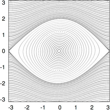
Figure 2: Iterates of the standard map $M_{\epsilon}$ (left) and of the time-$\epsilon$ map $\Phi^{\epsilon}_{X_{n}}$ associated to the interpolating vector field (with $n=5$) (right). In both cases $\epsilon=0.1$. No visual differences are detected in the plots.

In order to quantitatively describe the difference between the map and its interpolating flow, we consider interpolating vector fields $X_{n}$ for $n=5,10,15$ and $20$. Fig. 3 shows level plots of $|\Phi^{\epsilon}_{X_{n}}(x_{0})-M_{\epsilon}(x_{0})|$ computed for $5\times 10^{5}$ initial conditions selected on a uniform mesh in $[-\pi,\pi]\times[-2\pi,2\pi]$. We clearly see that the error vanishes at the fixed points of the map and that the error decreases as $n$ increases. Of course, the interpolation error will eventually grow with $n$ due to Runge oscillations in interpolation.

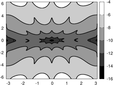
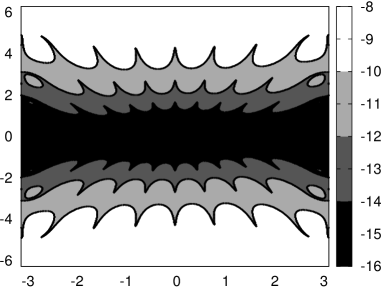
$n=5$                                            $n=10$

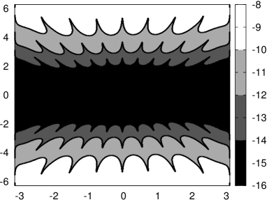
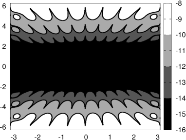
$n=15$                                          $n=20$

Figure 3: $\epsilon=0.1$. Level plots of $\log_{10}|\Phi^{\epsilon}_{X_{n}}(x_{0})-M_{\epsilon}(x_{0})|$ for $x_{0}\in[-\pi,\pi]\times[-2\pi,2\pi]$, and four different values of $n$.

Remark 3.1.

For the standard map (3.1), the interpolating flow $X_{n}$, for any $n$, defines a one degree of freedom Hamiltonian system (with a non-standard symplectic form). This follows from the fact that the map is reversible, hence so is the interpolating vector field, see Proposition 2.11. The reversibility of $X_{n}$ forces the phase space to be foliated by periodic orbits, see Fig. 2 right and also the right plots of Fig. 4 as illustrations. A reversible 2-dimensional system having a foliation of periodic orbits is Hamiltonian (possibly with a non-standard symplectic form).

To visually inspect the differences between the orbits for the map and the interpolating flow, we increase the parameter up to $\epsilon=0.5$ and show the results in Fig. 4. The left plots represent the iterates of the standard map $M_{\epsilon}$, while the right ones correspond to the time-$\epsilon$ map $\Phi^{\epsilon}_{X_{n}}$ for $n=10$. We recall that $X_{n}$ defines an integrable vector field, see Remark 3.1. The bottom raw of Fig. 4 shows magnifications of a part of the pictures from the top row: we can clearly see the differences between the phase portraits when magnifying a strip located near a chain of resonant islands of the map.

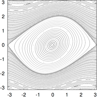
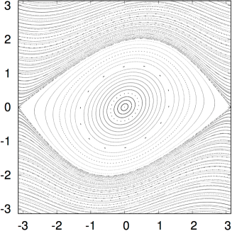
Figure 4: $\epsilon=0.5$. Left: Iterates of the standard map $M_{\epsilon}$. Right: Iterates of the time-$\epsilon$ map $\Phi^{\epsilon}_{X_{n}}$ (with $n=10$) associated to the interpolating vector field.

To study the adiabatic invariants defined by the equation (2.23), we fix a base point $x_{b}\in\mathbb{R}^{2d}$ ($d=1$ in this section but we will also use $d=2$ later) and consider paths represented by the function $\gamma(s,x_{b},x)=x_{b}+sv$ where $v=x-x_{b}$ and $0\leq s\leq 1$. Then the integral (2.23) takes the form

$$h_{n}(x,\epsilon)=\int_{0}^{1}\sum_{i=1}^{d}\left(X_{n}^{i}(\gamma(s,x_{0},x),\epsilon)v_{i+d}-X_{n}^{i+d}(\gamma(s,x_{0},x),\epsilon)v_{i}\right)ds$$ (3.2)

where $v_{i}$ are components of the vector $v$. In numerical experiments, we evaluate this integral using a trapezoidal rule combined with the Romberg extrapolation scheme. We accept a numerical estimate of the integral value if the difference between two consecutive approximations of the Romberg scheme is less than $10^{-8}$. We use this rule to evaluate the adiabatic invariants in all examples presented in the paper unless otherwise stated. In principle, this method can be used to achieve higher precision, however for the visualization purposes higher precision is not needed.

To investigate the preservation of the adiabatic invariants as a function of $n$ and $\epsilon$ under iterates of $M_{\epsilon}$, we select $10^{4}$ initial conditions which form a uniform mesh in $[-\pi,\pi]^{2}$ and for every point compute $\Delta h_{n}(x_{0})=|h_{n}(M_{\epsilon}(x_{0}),\epsilon)-h_{n}(x_{0},\epsilon)|$ and use the corresponding maximum value to estimate the supremum norm $\|\Delta h_{n}\|$.

(a)                                                            (b)

Figure 5: Plots of $\log_{10}\|\Delta h_{n}\|$: (a) as a function of $\log_{10}\epsilon$ for $1\leq n\leq 20$, and (b) as a function of $n$ for $\epsilon=0.1(0.1)0.5$.

Fig. 5(a) shows plots of $\|\Delta h_{n}\|$ as a function of $\log_{10}\epsilon$ for every $1\leq n\leq 20$. Each line of the plot corresponds to a fixed value of $n$ and is obtained by joining $50$ points with different values of $\epsilon\in[0,1/2]$. In this plot $n=1$ corresponds to the largest values of $\|\Delta h_{n}\|$. This plot confirms that the upper bound of Corollary 2.13 is not too far from being optimal as the lines on the plot are approximately linear with the slope about $2n+1$ (till they reach the levelled floor located just below $10^{-8}$, which is determined by our choice of the accuracy in evaluation of $h_{n}$). For $\epsilon\approx 0.15$ the values of $\|\Delta h_{n}\|$ are monotone decreasing for $1\leq n\leq 20$. On the other hand, we see that $\|\Delta h_{n}\|$ is not necessarily monotone in $n$ for larger values of $\epsilon$ as the lines have intersection. Moreover, the plot indicates that for a fixed $\epsilon$ the value of $\|\Delta h_{n}\|$ cannot be moved below a certain threshold by increasing the value of $n$ (see Fig 5(b)). Therefore for a fixed $\epsilon$ we can find an optimal value of $n$ which corresponds to a point after which the adiabatic invariant is not improved when $n$ is increased. The existence of this threshold can be attributed to the non-integrability of the map $M_{\epsilon}$. A similar phenomena are observed in the study of optimal truncation of asymptotic series.

Finally, we note that the methods of this section can be used to study some maps which are not a priori near identity but have an iterate which is near identity on some subset of the phase space. In particular, this situation can arise in a study of a near integrable system near a multiple resonance. For example, if $\epsilon$ is not small, the map $M_{\epsilon}$ is no longer close to identity. Nevertheless, in a neighbourhood of a $q$-periodic point, the map $M_{\epsilon}^{q}$ becomes close to identity. Let us illustrate how the interpolating vector field can be adapted to study the dynamics near a $q$-resonant chain of islands. Let $\epsilon=0.5$. We established (see Fig. 4) that the interpolating vector field provides an accurate approximation of the dynamics of $M_{\epsilon}$ for $y\in[-3,3]$. Now we consider larger values of $y$ and investigate what happens with the approximation. We take initial points with $x=\pi$ and iterate them. Comparing Fig 6 (a) and (b) which represent the dynamics of $M_{\epsilon}$ and the interpolating vector field $X_{n}$ for $n=5$, respectively, we see that the interpolating vector field does not correctly capture the dynamics around the 2-periodic chain of islands. On the other hand, in this part of the phase space the dynamics of $M_{\epsilon}^{2}$ is sufficiently close to identity so that the interpolating vector field $X_{2,n}$, computed from iterates of $M_{\epsilon}^{2}$, provides a good approximation of the dynamics as can be seen in Fig 6(c). Note, that only one of the two islands can be seen due to the choice of initial conditions.

(a)                                           (b)                                           (c)

Figure 6: $\epsilon=0.5$. Initial points taken on $x=\pi$, $n=5$. (a) Iterates of the standard map $M_{\epsilon}$, (b) Iterates of $\Phi^{\epsilon}_{X_{n}}$, and (c) Iterates of the map $\Phi^{\epsilon}_{X_{2,n}}$ associated with the interpolating vector field for $M_{\epsilon}^{2}$.

Fig. 7 shows similar results for $q=3$. Here we take initial points with $x=0$, hence only one of the 3-periodic islands appears in the picture. The interpolating vector field $X_{n}^{3}$ computed for $M_{\epsilon}^{3}$ accurately describes the dynamics in a narrow zone around the resonant 3-periodic island. Note that the 5-periodic island observed in Fig. 7(a) is not present in Fig. 7(b).

(a)                                                            (b)

Figure 7: $\epsilon=0.5$. Initial points taken on $x=0$, $n=5$. (a) Iterates of the standard map, and (b) iterates of $\Phi^{\epsilon}_{X_{3,n}}$ associated to the interpolating vector field for $M_{\epsilon}^{3}$.

3.2 Exploring higher dimensional phase spaces: Poincaré sections for maps

If the dimension of the phase space $m\geq 3$, the visualization of the dynamics becomes more difficult. In the case of a system with continuous time, a Poincaré section provides a convenient tool to reduce the dimension: a trajectory is represented by its intersections with a codimension one surface. In the case of discrete time, the reduction of the dimension cannot be performed in a similar way. A typical solution to this problem is either to plot a projection of the trajectory on a subset of lower dimension, or to use the method of slices [9], i.e. to plot only a part of the trajectory which consists of points from a narrow strip near a codimension one surface (called a slice). In the last case, the points are also projected on the surface to reduce the dimension.

The interpolating vector fields provide a new tool for visualization of dynamics which is especially effective in dimensions three and four. Suppose that $g:\mathbb{R}^{m}\to\mathbb{R}$ is a smooth function such that its zero set $\Sigma=\{x\in\mathbb{R}^{m}:g(x)=0\}$ is a smooth hyper-surface of codimension one. Taking an initial condition $x_{0}\in D$ we compute the points $x_{k+1}=F_{\epsilon}(x_{k})$ recursively. The surface $\Sigma$ locally divides the space. So we can look for consecutive points of the trajectory which are separated by $\Sigma$, i.e.,

$$g(x_{k})g(x_{k+1})\leq 0.$$ (3.3)

Suppose that the limit vector field $G_{0}$ is transversal to $\Sigma$ (at least in a neighbourhood of the intersection of $\Sigma$ with the straight segment with endpoints at $x_{k}$ and $x_{k+1}$). Then, for $\epsilon$ small enough, there is a unique $t_{k}\in[0,\epsilon]$ such that $g(\Phi_{X_{n}}^{t_{k}}(x_{k}))=0$, and we plot the point

$$y_{k}=\Phi_{X_{n}}^{t_{k}}(x_{k})$$ (3.4)

instead of $x_{k}$. Obviously, $y_{k}\in\Sigma$ and the trajectory is represented on a manifold of lower dimension. The point $y_{k}$ is $O(\epsilon)$ close to $x_{k}$ and the error does not accumulate when $k$ grows as the construction of $y_{k}$ does not affect the computation of the trajectory $(x_{k})_{k\geq 0}$.

3.3 Four-dimensional symplectic maps: the Froechlé-like map

We apply the construction of the previous section to a 4-dimensional symplectic map and show that the method reveals interesting details of the dynamics. We consider the Froechlé-like map

$$T_{\epsilon}:\left(\begin{array}[]{c}\psi_{1}\\ \psi_{2}\\ J_{1}\\ J_{2}\end{array}\right)\mapsto\left(\begin{array}[]{c}\bar{\psi}_{1}\\ \bar{\psi}_{2}\\ \bar{J}_{1}\\ \bar{J}_{2}\end{array}\right)=\left(\begin{array}[]{c}\psi_{1}+\epsilon(a_{1}\bar{J}_{1}+a_{2}\bar{J}_{2})\\ \psi_{2}+\epsilon(a_{2}\bar{J}_{1}+a_{3}\bar{J}_{2})\\ J_{1}-\epsilon\sin(\psi_{1})\\ J_{2}-\epsilon\eta\sin(\psi_{2})\end{array}\right),$$ (3.5)

where $a_{1},a_{2},a_{3},\eta,\epsilon$ are real parameters. The map $T_{\epsilon}$ is a symplectic diffeomorphism of the cylinder $M=\mathbb{T}^{2}\times\mathbb{R}^{2}$. It was introduced in [6] to model the dynamics near a double resonance in a near-integrable Hamiltonian system with three degrees of freedom. In our numerical experiments we use

$$a_{1}=1,\qquad a_{2}=1/2,\qquad a_{3}=5/4,\qquad\eta=1/2.$$ (3.6)

The quadratic form $a_{1}J_{1}^{2}+2a_{2}J_{1}J_{2}+a_{3}J_{2}^{2}$ is positive definite, since $a_{3}-a_{2}^{2}>0$. The map (3.5) has four fixed points. If $\epsilon$ is positive and not too large, the origin $p_{1}=(0,0,0,0)$ is elliptic-elliptic, $p_{2}=(0,\pi,0,0)$ and $p_{3}=(\pi,0,0,0)$ are hyperbolic-elliptic and $p_{4}=(\pi,\pi,0,0)$ is hyperbolic-hyperbolic.

A Poincaré section for $T_{\epsilon}$

Since the map (3.5) is symplectic, its limit flow is Hamiltonian. It is easy to find the corresponding Hamiltonian function explicitly:

$$h_{0}(\psi_{1},\psi_{2},J_{1},J_{2})=a_{1}\frac{J_{1}^{2}}{2}+a_{2}J_{1}J_{2}+a_{3}\frac{J_{2}^{2}}{2}-\cos(\psi_{1})-\eta\cos(\psi_{2}).$$ (3.7)

This Hamiltonian defines a non-integrable Hamiltonian system with two degrees of freedom. The Hamiltonian $h_{0}$ has four critical points which coincide with the fixed points of $T_{\epsilon}$. Levels of constant energy, $M_{E}^{0}=\{x:h_{0}(x)=E\}$, are smooth hyper-surfaces for every regular value of $h_{0}$. It is natural to study the dynamics of the limit system restricted on each energy level separately as the Hamiltonian function $h_{0}$ remains constant along trajectories of the limit flow. Let $\Sigma$ be the 3-dimensional hyper-surface defined by the equality $\psi_{1}=\psi_{2}$. Note that we do not call $\Sigma$ a “hyper-plane” because we treat $\psi_{1}$ and $\psi_{2}$ as angular variables. The limit vector field is transversal to $\Sigma$ except for points which satisfy the equation $(a_{1}-a_{2})J_{1}=(a_{3}-a_{2})J_{2}$ where the vector field is tangent to $\Sigma$.

The intersection $\Sigma^{0}_{E}=\Sigma\cap M_{E}^{0}$ defines a Poincaré section for the limit flow. Outside a neighbourhood of the tangencies, the first return map of the limit flow defines an area-preserving map on $\Sigma^{0}_{E}$. The dynamics of the limit Hamiltonian system are described by a collection of the Poincaré sections for different values of $E$. Since the quadratic form $a_{1}\frac{J_{1}^{2}}{2}+a_{2}J_{1}J_{2}+a_{3}\frac{J_{2}^{2}}{2}$ is positive definite, $M_{E}^{0}$ is diffeomorphic to a three dimensional torus $\mathbb{T}^{3}$ for every $E>h_{0}(p_{4})=1+\eta$. Then $\Sigma_{E}^{0}$ is diffeomorphic to a two dimensional torus $\mathbb{T}^{2}$. It is convenient to use $\psi=\psi_{1}=\psi_{2}$ and $\phi=\arg(J_{1}+iJ_{2})$ as coordinates on $\Sigma_{E}^{0}$.

In contrast to the limit flow, the map $T_{\epsilon}$ does not have a first integral. Moreover, even if $x_{0}\in\Sigma$, it is unlikely that $x_{k}=T_{\epsilon}^{k}(x)$ will ever come back to $\Sigma$ (periodic points of $T_{\epsilon}$ are obvious exceptions) so the direct implementation of the Poincaré section is not possible. In order to visualise a trajectory $x_{k}=T_{\epsilon}^{k}(x_{0})$ we implement the procedure explained in Section 3.2. The procedure consists in finding a subsequence $k_{j}$ such that the trajectory jumps over $\Sigma$ between $x_{k_{j}}$ and $x_{k_{j}+1}$. We note that $\Sigma$ does not divide the cylinder $M$ into two subsets globally but, since the map $T_{\epsilon}$ is near identity, we can check this condition locally. Since $\Sigma$ is defined by the equality $\psi_{1}=\psi_{2}$, we look for $k_{j}$ such that $(\psi_{1}^{k_{j}}-\psi_{2}^{k_{j}})(\psi_{1}^{k_{j}+1}-\psi_{2}^{k_{j}+1})<0$, where $x_{k}=(\psi_{1}^{k},\psi_{2}^{k},J_{1}^{k},J_{2}^{k})$ denotes the $k$-th iterate of $x_{0}\in\mathbb{T}^{2}\times\mathbb{R}^{2}$. Then a point $y_{k_{j}}\in\Sigma$ is defined by projecting $x_{k_{j}}$ to $\Sigma$ along the interpolating vector field $X_{n}$ as defined by the equation (3.4).

Since the section $\Sigma$ is three dimensional, the sequence $y_{k_{j}}$ can be plotted and used to visually inspect the behaviour of the trajectory $x_{k}$.

On a moderate time scale, a further reduction of the dimension can be achieved by noting that $h_{n}$ (defined by the equation (3.2)) is an adiabatic invariant of the map, so the trajectory $x_{k}$ stays in a small neighbourhood of the set $M_{E}^{n}=\{x:h_{n}(x,\epsilon)=E\}$ where $E=h_{n}(x_{0},\epsilon)$. Since $M_{E}^{n}$ is close to $M_{E}^{0}$ and the latter is nicely described by the coordinates $(\psi,\phi)$, we can project the points $y_{k_{j}}$ on the torus of the coordinates $(\psi,\phi)$. In this way a trajectory of a 4-dimensional map is represented by a sequence of points on a two dimensional torus.

We remark that this procedure relies on the closeness of the map to the identity. Similar to the standard map, acceptable values of $\epsilon$ depend on the values of the variables $J_{1}$ and $J_{2}$. In our numerical experiments we use $|\epsilon|\leq 0.5$, so in practical terms the parameter does not need to be very small.

Visualization of the dynamics of $T_{\epsilon}$

Examples of visualization of dynamics for $T_{\epsilon}$ are shown on Fig. 1 and 8. Some comments concerning the implementation can help the reader. First, the computation of the points $y^{k_{j}}$ on $\Sigma$ requires integration of $X_{n}$ which is performed using a RK7-8 method that only requires evaluating the vector field. The time $t_{k}$ in (3.4) is then computed using the Newton method in a way similar to [10].

Second, to show different trajectories on a single 2-dimensional torus we select initial conditions on $\Sigma_{E}^{n}=\Sigma\cap M_{E}^{n}$ for a fixed $E$. To find initial conditions with the same value of $E$, we use the following procedure: we select values of $\psi=0,1,2,3$ and, for each value, we compute a point $p=(\psi,\psi,0,J_{2}^{0})$, with $J_{2}^{0}>0$, such that $h_{n}(p,\epsilon)=E$ (using a bisection method with respect to $J_{2}$ to get a zero of $h_{n}(p,\epsilon)-E$). Since $\nabla h_{n}$ is orthogonal to the vector $(0,0,-\partial h_{n}/\partial J_{2},\partial h_{n}/\partial J_{1})$, we numerically integrate the auxiliary vector field

$$\dot{J}_{1}=-\frac{\partial{h_{n}}}{\partial J_{2}}\,,\qquad\dot{J}_{2}=\frac{\partial{h_{n}}}{\partial J_{1}}\,,$$ (3.8)

with initial condition $(J_{1}(0),J_{2}(0))=(0,J_{2})$ (using a RK7-8 method). One obtains points $x_{0,i}=(\psi,\psi,J_{1}(t_{i}),J_{2}(t_{i}))\in\Sigma^{n}_{E}$ for a sequence of $t_{i}$ provided by the integration method. Finally, we use $x_{0,i}$ as initial conditions for the map $T_{\epsilon}$.

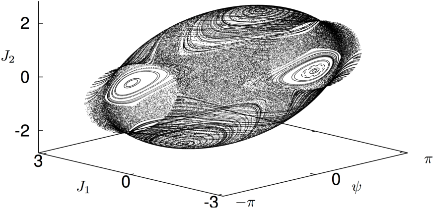
(a)

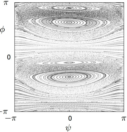
(b)(c)

Figure 8: Trajectories of $T_{\epsilon}$ with the parameters defined by (3.6) and $\epsilon=0.2$, $E=1$, $n=10$. (a) $500$ projections $y_{k_{j}}$ are plotted for each of $400$ initial conditions taken on $\Sigma\cap M^{n}_{E}$, (b) projection of the points of (a) onto the torus with coordinates $(\psi,\phi)$, where $\phi=\arg(J_{1}+iJ_{2})\in(-\pi,\pi]$, (c) is a magnification from (b).

Fig. 8 shows 500 projected iterates $y_{k_{j}}$, as defined by (3.4), obtained from the iterates $x_{k_{j}}$ under the map $T_{\epsilon}$ for each of around 400 different initial conditions. The parameters of the map are defined by (3.6) and $\epsilon=0.2$. The hyperbolic-hyperbolic fixed point $p_{4}$ is used as a base point $x_{b}$ in the definition of the adiabatic invariant and the initial conditions are chosen on $M_{E}^{n}$ with $n=10$ and $E=1$. We see that all points are located near a 2-dimensional torus embedded in the 3-dimensional surface $\Sigma$. The projection of the trajectories onto the coordinates $(\psi,\phi)$ resembles the dynamics of an area-preserving map.

(a)(b)

(c)(d)

Figure 9: A single trajectory of the map $T_{\epsilon}$ with $\epsilon=0.2$ for the initial point located at $(3,3,-1.043523,1.385456)$. (a) Points on the Poincaré section are represented using coordinates $\psi_{1}\ (=\psi_{2})$ and $\phi=\arg(J_{1}+iJ_{2})\in(-\pi,\pi]$; we show only one out of every ten consecutive points on the Poincaré section. (b) The adiabatic invariant $h_{n}$ as a function of time (we show one point out of every 250 iterates). (c) The same as in (b) but up to $10^{10}$ iterates instead (we show one point out of every $250\times 10^{4}$ iterates). (d) A histogram which illustrates the distribution of the adiabatic invariant for the Poincaré iterates up to $t=10^{6}$. The values of $E$ for the $10^{6}$ iterates considered range in $[-10^{4},10^{4}]$ and a bin size of $8\times 10^{-7}$ has been used to obtain the distribution.

Fig. 9(a) shows iterates of the point $(\psi_{1},\psi_{2},J_{1},J_{2})=(3,3,-1.043523,1.385456)$ that belongs to $\Sigma_{E}^{n}$ with $E=1$. This is one of the chaotic orbits which can be seen in Fig. 8. Fig. 9(b) shows a plot of the adiabatic invariant as a function of time along this orbit. For better visualization we show the value of the adiabatic invariant for one out of every 250 consecutive iterates of the point under $T_{\epsilon}$. Some important observations follow from this plot:

• The orbit we study apparently belongs to a chaotic zone and is not located on a KAM torus.

• The adiabatic invariant is preserved (meaning that the range of oscillations remains unchanged) up to, at least, $10^{6}$ iterates. Fig. 9(c) shows that this behaviour continues at least for $10^{10}$ iterates of $T_{\epsilon}$. The dynamical interpretation of such preservation is clear: our numerical method has detected the slowest variable of the system which evolves on a very long time scale. We note that in this example one expects to see an (Arnold like) diffusion process and, in particular, the slow variable requires exponentially long (with respect to $\epsilon^{-1}$) time to be changed by order one. Our method is able to detect such a slow variable in a simple and efficient way.

• There is no systematic drift of the adiabatic invariant. Its values are distributed in a Gaussian-like way around the initial value (see Fig. 9(d)). We remark that, for $T_{\epsilon}$ and the chosen parameters, there is numerical evidence supporting that the detection of the expected drift in the adiabatic invariant due to the Arnold diffusion process requires a much longer time scaling.

A final illustration of the amount of details one can visualize with this methodology is presented in Fig. 1. There we show a plot similar to the one in Fig. 8 but for $\epsilon=0.35$ and $E=4$. As before, we take the hyperbolic-hyperbolic fixed point $p_{4}$ as a base point to define the adiabatic invariant. The interpolating vector field is constructed with $n=10$. One can clearly recognize the typical structures that show up in a phase space of an area-preserving map: islands of stability (including secondary islands and satellites in the chaotic zone), invariant curves and chaotic zones. Yet this is not a 2-dimensional map: we are just plotting a suitable projection (along the solutions of the interpolating vector field) of the iterates of the 4-dimensional map!

4 Acknowledgments

AV has been supported by grants MTM2016-80117-P (Spain) and 2014-SGR-1145 (Catalonia). VG’s research was supported by EPRC (grant EP/J003948/1). The authors are grateful to Ernest Fontich and Carles Simó for useful discussions and remarks.

References

- [1] Bogoliubov, N. N., Mitropolsky, Y. A.; Asymptotic methods in the theory of non-linear oscillations. Gordon and Breach Science Publishers, New York 1961, 537 pp.
- [2] Broer, H., Roussarie, R., and Simó, C.; Invariant circles in the Bogdanov-Takens diffeomorphisms. Ergod. Th. and Dynam. Sys., 16:1147 – 1172, 1996.
- [3] Chirikov, B.V.; A universal instability of many-dimensional oscillator system. Phys. Rep., 52 (1979), 264–379.
- [4] Efthymiopoulos, C., and Harsoula, M.; The speed of Arnold diffusion, Physica D vol. 251 issue 1 (2013) pp. 19–38.
- [5] Gelfreich, V., Numerics and exponential smallness. In Handbook of dynamical systems, Vol. 2, 265–312, North-Holland, Amsterdam, 2002.
- [6] Gelfreich, V., Simó, C., and Vieiro A.; Dynamics of 4D symplectic maps near a double resonance, Physica D vol. 243 issue 1 (2013) pp. 92–110.
- [7] Neishtadt, A.I.; The separation of motions in systems with rapidly rotating phase, J.Appl. Math. Mech., 48 (1984), 133–139.
- [8] Nekhoroshev N.N.; An exponential estimate of the time of stability of nearly integrable Hamiltonian systems. Russian Mathematical Surveys, 32(6) (1977) 1–65.
- [9] Richter M., Lange S., Bäcker A, Ketzmerick R.; Visualization and comparison of classical structures and quantum states of four-dimensional maps. Phys. Rev. E 89(2) (2014) 022902
- [10] Simó, C.; On the Analytical and Numerical Approximation of Invariant Manifolds, Les Méthodes Modernes de la Mecánique Céleste (Course given at Goutelas, France, 1989), D. Benest and C. Froeschlé (eds.), pp. 285–329, Editions Frontières, Paris, 1990.
- [11] Simó, C.; Analytic and numeric computations of exponentially small phenomena, In K. Gröger B. Fiedler and J. Sprekels, editors, Proceedings EQUADIFF 99, Berlin, pages 967 – 976, 2000. World Scientific, Singapore.
- [12] Stoer, J; and Bulirsch, R.; Introduction to Numerical Analysis. Third edition. Texts in Applied Mathematics, 12. Springer-Verlag, New York, 2002. xvi+744 pp.
- [13] Takens, F.; Forced oscillations and bifurcations, Applications of Global Analysis I. Communications of the Mathematical Institute Rijksuniversiteit Utrecht, 3, 1974.