Intrinsic Entropy Perturbations from the Dark Sector

Marco Celoria^a, Denis Comelli^b, Luigi Pilo^c,d
a Gran Sasso Science Institute (INFN)
Via Francesco Crispi 7, L’Aquila, I-67100
^bINFN, Sezione di Ferrara, I-35131 Ferrara, Italy
^cDipartimento di Fisica, Università dell’Aquila, I-67010 L’Aquila, Italy
^dINFN, Laboratori Nazionali del Gran Sasso, I-67010 Assergi, Italy
marco.celoria@gssi.infn.it, comelli@fe.infn.it, luigi.pilo@aquila.infn.it

Abstract

Perfect fluids are modeled by using an effective field theory approach which naturally gives a self-consistent and unambiguous description of the intrinsic non-adiabatic contribution to pressure variations. We study the impact of intrinsic entropy perturbation on the superhorizon dynamics of the curvature perturbation ${\cal R}$ in the dark sector. The dark sector, made of dark matter and dark energy is described as a single perfect fluid. The non-perturbative vorticity’s dynamics and the Weinberg theorem violation for perfect fluids are also studied.

1 Introduction

The Universe is undergoing a phase of accelerated expansion [1, 2]. What is is driving such an accelerated phase is presently not known and a number of forthcoming dark energy surveys will try to shed some light on its nature, see for instance [3, 4, 5, 6]. Besides the cosmological constant, a vast number of models have been proposed, ranging from proposals of modifications of gravity to the addition of exotic matter. Unfortunately, only a small number of observables are available from the surveys and discriminating among the various models is going to be very challenging. For this reason it important to build the simplest possible effective description for a dark fluid that is able to capture all the relevant physical properties distinguishing dark energy from cosmological constant. Recently [7, 8] is has been proposed an effective description of dark sector modelled as a generic self-gravitating medium. Such a medium is described by the theory of four derivatively coupled scalar which can be interpreted as comoving coordinates of the medium whose fluctuations represent the Goldstone modes for the broken spacetime translations. The very same scalar fields can be viewed as Stückelberg fields that allow to restore broken diffeomorphisms  [9, 10, 11, 7, 12, 13]. Such an effective field theory description has been already considered in [14, 15, 16, 17] for particular type of media. Internal symmetries of the medium action determine both the dynamical and the thermodynamical properties of the system. In the present study we will focus on the phenomenological consequences of taking dark energy as the simplest class of self-gravitating media: perfect fluids. Though perfect fluids are rather simple, taking into account a non-barotropic equation of state leads to an additional source in the growth of structure and to the dynamics of the comoving curvature perturbation ${\cal R}$. The effective field theory description allows us to determine in a consistent and compact way the form of the non-adiabatic contributions induced by pressure variations. The formalism is also employed to study when the Weinberg Theorem [18, 19] is violated.
The outline of the paper is the following. In section 2 we introduce the effective action which gives the non perturbative dynamical description of a generic non-barotropic perfect fluid, together with the relation among thermodynamical variables and field theory operators; in relation with previous literature, [20, 21], at non-perturbative level, the influence of entropy on the time evolution the fluid’s vorticity. Section 3 is devoted to linear cosmological perturbations in a flat FRW Universe in the presence of a single entropic perfect fluid by using its effective field theory description. We analyse also the conditions for the violation of Weinberg theorem [18, 19] in the presence of perfect fluids, confirming and extending the known results. Such results are extended to multifluids in section 4. The phenomenological consequences of the entropic modes are considered for different descriptions of the dark sector. The $\Lambda$CDM model described in section 5.1 is compared with different fluid models of the dark sector in sections 6.1, 6.2, 6.3. Our conclusions are given in section 7.

2 Perfect Fluids Action and Thermodynamics

Perfect fluids and non dissipative general media can be described by using an effective field theory approach in terms of four scalar fields $\Phi^{A}$ ($A=0,1,2,3$). The medium physical properties are encoded in a set of symmetries of the scalar field action selecting, order by order in a derivative expansion, a finite number of operators. Following [7, 22] we require the Lagrangian to be invariant under:

$$\begin{split}\text{global shift symmetries:}&\quad\Phi^{A}\to\Phi^{A}+f^{A}\,;\\ \text{field dependent symmetries:}&\quad\Phi^{0}\to\Phi^{0}+f(\Phi^{a});\quad\Phi^{a}\to f^{a}(\Phi^{b}),\quad\det\left|\frac{\partial f^{a}}{\partial\Phi^{b}}\right|=1\,;\\ \text{internal rotational invariance:}&\quad\Phi^{a}\to{\cal M}^{a}_{b}\;\Phi^{b}\,,\quad{\cal M}\in\text{SO}(3)\,.\end{split}$$ (2.1)

The global shift symmetry requires the scalars appear in the action only through their derivatives, while field dependent symmetries plus internal rotational invariance select the following operators

$$b=\left[\det\left(g^{\mu\nu}\partial_{\mu}\Phi^{a}\,\partial_{\nu}\Phi^{b}\right)\right]^{1/2},\qquad u^{\mu}=\frac{1}{b\;\sqrt{g}}\epsilon^{\mu\alpha\beta\gamma}\;\partial_{\alpha}\Phi^{1}\;\partial_{\beta}\Phi^{2}\;\partial_{\gamma}\Phi^{3},\qquad Y=u^{\mu}\;\partial_{\mu}\Phi^{0}\,;$$ (2.2)

with $u^{2}\equiv u^{\mu}u_{\mu}=-1$. As a result, our starting point is the most general action given by

$$S=\int d^{4}x\;\sqrt{g}\;U(b,\,Y)\,;$$ (2.3)

that gives the following conserved energy momentum tensor (EMT)

$$T_{\mu\nu}=\rho\;u_{\mu}\;u_{\nu}+(\rho+p)\;g_{\mu\nu}\,,$$ (2.4)

with a perfect fluid form where 

$$\rho=-U+Y\;U_{Y},\qquad p=U-b\;U_{b}\,.$$ (2.5)

The shift symmetries (2.2) lead to the existence of two conserved currents 

$$\nabla^{\mu}J_{\mu}=\nabla^{\mu}(b\,u_{\mu})=\dot{b}+\theta\;b=0\,;$$ (2.6)

$$\nabla^{\mu}{\cal J}_{\mu}=\nabla^{\mu}(U_{Y}\,u_{\mu})=\dot{U}_{Y}+\theta\;U_{Y}=0\,;$$ (2.7)

where $\dot{f}=u^{\nu}\nabla_{\nu}f$ is the Lie derivative of $f$ along $u^{\mu}$. It also follows from (2.6, 2.7) that the ratio $\sigma\equiv\frac{U_{Y}}{b}$ is conserved, indeed

$$u^{\mu}\nabla_{\mu}\,\sigma\equiv\dot{\sigma}=0\,.$$ (2.8)

The equations (2.6, 2.7) are equivalent to the projection of the EMT conservation (2.4) along $u^{\mu}$.

One can also relate the operators $b$ and $Y$ with thermodynamical variables of the fluid, namely the entropy density $s$, the chemical potential $\mu$ and the temperature $T$. The basic input is the first principle $d\rho=T\;ds+\mu\;dn$ and the Euler Relation $\rho=T\;s-p+\mu\;n$ or equivalently the Gibbs-Duhem equation $dp=s\,dT-n\,d\mu$. As shown in  [22], two consistent thermodynamical interpretation relating the operators $b$ and $Y$ and thermodynamical variables exist, namely

$$T=Y,\qquad s=U_{Y},\qquad n=b\qquad\mu=-U_{b}\,;$$ (2.9)

$$T=-U_{b},\qquad s=b,\qquad n=U_{Y}\qquad\mu=Y\,.$$ (2.10)

where we neglect a constant normalisation factor for each equality. For the rest of the paper we will consider the relationship (2.9). From (2.9), the conserved quantity $\sigma=\frac{s}{n}$ (see eq.(2.8)) is the entropy per particle and it is always conserved for perfect fluids. The current

$$J_{\mu}=b\;u_{\mu}$$ (2.11)

is always conserved independently from the equations of motion of the scalar fields, with $b=n$ representing the number particle density.
The hydrodynamic equations for a perfect fluid are equivalent to the EMT and current conservation

$$\nabla^{\nu}T_{\mu\nu}=0\,,\qquad\nabla^{\mu}J_{\mu}=0\,.$$ (2.12)

Indeed, projecting the EMT conservation equation along $u^{\mu}$ and on an orthogonal direction by using the projector $h_{\mu}^{\nu}=\delta_{\mu}^{\nu}+u_{\mu}\,u^{\nu}$, we have that

$$\dot{\rho}+\theta\;(p+\rho)=0,\qquad D_{\mu}\,p=-(p+\rho)a_{\mu}\;$$ (2.13)

where

$$\theta=\nabla_{\mu}\,u^{\mu}\,,\qquad D_{\mu}=h_{\mu}^{\nu}\,\nabla_{\nu}\,,\qquad a_{\mu}=u^{\nu}\nabla_{\nu}u_{\mu}\,.$$ (2.14)

The study of the differential properties of the pressure allows to single out the non adiabatic contribution $\mathbf{\Gamma}$  [23]. Indeed, knowing $p$ as function of $b$ and $Y$ by eq (2.5) and using (2.9) we can express $p$ also as a function of $\rho$ and $\sigma$, thus

$$dp=\left.\frac{\partial p}{\partial\rho}\right|_{\sigma}\;d\rho+\left.\frac{\partial p}{\partial\sigma}\right|_{\rho}\;d\sigma\;\equiv\;c_{s}^{2}\;d\rho+\mathbf{\Gamma}\,;$$ (2.15)

$c_{s}^{2}$ is the adiabatic sound speed. Notice that the definition (2.15) of $\mathbf{\Gamma}$ is general and non perturbative.

The EFT description together with the thermodynamical dictionary (2.9) allow us to compute explicitly $\mathbf{\Gamma}$. From the knowledge of $p$, $\rho$ and $\sigma$ as function of $b$ and $Y$, the 1-forms $d\,b$ and $d\,Y$ can be expressed in terms of $d\,\rho$ and $d\,\sigma$. Actually, $c_{s}^{2}$ can be computed in a simpler way by contracting the 1-form $d\,p$ with $u^{\mu}$ to get

$$d\,p(u)=u^{\mu}\partial_{\mu}p=\dot{p}=c_{s}^{2}\;\dot{\rho}+\left.\frac{\partial p}{\partial\sigma}\right|_{\rho}\,\dot{\sigma}=c_{s}^{2}\;\dot{\rho}\,,\qquad{\rm being}\;\;\;\dot{\sigma}=0\,;$$ (2.16)

thus

$$c_{s}^{2}=\left.\frac{\partial p}{\partial\rho}\right|_{\sigma}=\frac{\dot{p}}{\dot{\rho}}=\frac{p_{b}\,\dot{b}+p_{Y}\,\dot{Y}}{\rho_{b}\,\dot{b}+\rho_{Y}\,\dot{Y}}=\frac{(U_{Y}-b\;U_{bY})^{2}-b^{2}\;U_{b^{2}}\;U_{Y^{2}}}{{U_{Y^{2}}}\;(\rho+p)}\,;$$ (2.17)

where we have used (2.6) and (2.7) to eliminate $\dot{b}$ and $\dot{Y}$. For ${\mathbf{\Gamma}}$ we get

$$\mathbf{\Gamma}=\left.\frac{\partial p}{\partial\sigma}\right|_{\rho}\,d\,\sigma\equiv c_{\rho}^{2}\;d\,\sigma=b\;Y\;(c_{b}^{2}-c_{s}^{2})\,d\,\sigma\,.$$ (2.18)

with

$$c_{\rho}^{2}\;=\left.\frac{\partial p}{\partial\sigma}\right|_{\rho}=b\;Y\;(c_{b}^{2}-c_{s}^{2})\;\qquad c_{b}^{2}=\left.\frac{\partial p}{\partial\rho}\right|_{b}=\left.\frac{\partial p}{\partial\rho}\right|_{n}=\frac{U_{Y}-b\;U_{bY}}{Y\;U_{Y^{2}}}\,.$$ (2.19)

From the conservation of ${\cal J}_{\mu}$ one can derive an evolution equation for $Y$; expanding (2.7) and using (2.6) to eliminate $\dot{b}$, one gets by using the definition (2.19) of $c_{b}^{2}$

$$\dot{Y}=-c_{b}^{2}\;\theta\;Y\,;$$ (2.20)

in addition (2.7) and (2.6) can be rewritten as

$$\frac{\dot{U}_{Y}}{U_{Y}}=\frac{\dot{b}}{b}\,.$$ (2.21)

Finally, by contracting $d\,p$ with the orthogonal projector $h_{\mu}^{\nu}$ one gets

$$D_{\alpha}\,p=c_{s}^{2}\;D_{\alpha}\rho+c_{\rho}^{2}\,D_{\alpha}\,\sigma\,;$$ (2.22)

where $D_{\mu}f=h_{\mu\nu}\,\nabla^{\nu}f$ is the projected covariant derivative acting on a scalar function $f$. Once the perfect fluid is specified giving $U(b,Y)$, one can compute $c_{s}^{2}$, $c_{b}^{2}$ and $c_{\rho}^{2}$, then $\mathbf{\Gamma}$ is known in a fully non perturbative way. As we will see the knowledge of $\mathbf{\Gamma}$ is crucial to study the dynamics of the gravitational potential in a perturbed Friedman Lemaitre Robertson Walker (FLRW) Universe.

In [24, 25] it was shown that it is possible to give a non perturbative gauge invariant definition of entropic variables, defining appropriate spatial-gradient quantities, leading to simple geometric nonlinear conserved quantities for a perfect fluid

$$\zeta_{a}\equiv D_{a}\alpha-\frac{\dot{\alpha}}{\dot{\rho}}\;D_{a}\rho=D_{a}\alpha+\frac{D_{a}\rho}{3\;(\rho+p)}\;,\qquad\theta=3\;\dot{\alpha}\,.$$ (2.23)

The “evolution” equation for the $\zeta_{a}$ vector is given by the following Lie derivative obtained using the equations of motion of the perfect fluid (2.13) (the Lie derivative of a 1-form is given by ${\cal L}_{u}(\zeta_{a})=\;\zeta_{a}^{\prime}+\zeta_{b}\;\nabla_{a}\;u^{b}$)

$${\cal L}_{u}(\zeta_{a})=-\frac{\theta}{3\;(\rho+p)}\left(D_{a}p-\frac{\dot{p}}{\dot{\rho}}\;D_{a}\rho\right)\,.$$ (2.24)

This result is valid for any spacetime geometry and does not depend on Einstein’s equations. In the cosmological context, $\alpha$ can be interpreted as a non-linear generalisation, according to an observer following the fluid, of the number of e-folds of the scale factor. On scales larger than the Hubble radius, the above definitions are equivalent to the non-linear curvature perturbation on uniform density hypersurfaces [24]. From (2.22) and (2.18) we can write

$${\cal L}_{u}(\zeta_{a})=-\frac{\theta\;c_{\rho}^{2}}{3\;(\rho+p)}\;D_{a}\sigma=-\frac{\theta\;n\;T\,(c_{b}^{2}-c_{s}^{2})}{3\;(\rho+p)}\;D_{a}\sigma\quad{\rm with}\quad\dot{\sigma}=0\,.$$ (2.25)

For isentropic perturbations, $D_{\alpha}\sigma=0$, (2.24) vanishes identically and the above guarantees that ${\cal L}_{u}(\zeta_{a})=0$, i.e. $\zeta_{a}$ is a conserved quantity in the isentropic/barotropic case on all scales and at all perturbative orders. By defining the vorticity tensor $\Omega_{\alpha\beta}$, the enthalpy $h$ and the enthalpy vector $w_{\alpha}$ as

$$h=\frac{p+\rho}{n}\,,\qquad w_{\alpha}=h\;u_{\alpha}\,,\qquad\Omega_{\alpha\beta}\equiv\nabla_{\beta}\;w_{\alpha}-\nabla_{\alpha}\;w_{\beta}$$ (2.26)

we note that the spatially projected EMT conservation equation can be also rewritten in form

$$\Omega_{\alpha\beta}\,u^{\beta}=T\;D_{\alpha}\sigma$$ (2.27)

as proposed by Carter and Lichnerowicz [26, 27], As a consequence, if a perfect fluid has zero vorticity tensor, i.e $\Omega_{\mu\nu}=0$, then equation (2.27) immediately implies that irrotational perfect fluids are also isentropic. From the definition of $\Omega_{\alpha\beta}$ it follows that if the vorticity is zero, then the velocity of a relativistic (isentropic) perfect fluid can be expressed as the gradient of a velocity potential function. More specifically, the enthalpy current can be expressed, at least locally, as the gradient of a potential $F$, $w_{\mu}=h\;u_{\mu}=\nabla_{\mu}\;F$. Of course, an isentropic fluid does not necessarily have zero vorticity. Equation (2.25) can also be rewritten in the form

$${\cal L}_{u}(\zeta_{\alpha})=-\frac{\theta\;(c_{b}^{2}-c_{s}^{2})}{h}\;\Omega_{\alpha\beta}\;u^{\beta}\,.$$ (2.28)

A physical observable that is particularly sensitive to entropic perturbations is the kinematic vorticity tensor and the kinematic vorticity vector, defined as

$$\omega_{\mu\nu}=\frac{1}{2}\;\left(D_{\mu}u_{\nu}-D_{\nu}u_{\mu}\right),\quad\omega^{\mu}=\frac{1}{2}\;\epsilon^{\mu\alpha\beta\gamma}\;u_{\gamma}\;\omega_{\alpha\beta}$$ (2.29)

whose non-perturbative time evolution equation is given by [20, 21]

$$h^{\nu}_{\mu}\;\dot{\omega}_{\nu}=-\frac{2}{3}\;\theta\;\omega_{\mu}+\sigma_{\mu\nu}\;\omega^{\nu}-\frac{1}{2}\;{\rm curl}(a_{\mu})\,;$$ (2.30)

where ${\rm curl}(a_{\mu})=\epsilon_{\mu\alpha\beta}\,D^{\alpha}\,a^{\beta}$ and $\epsilon_{\mu\alpha\beta}=\epsilon_{\mu\alpha\beta\gamma}\;u^{\gamma}$ and ${\rm curl}(D_{\mu}f)=-2\;\dot{f}\;\omega_{\mu}$.
By using the following relations

$${\rm curl}(D_{\mu}p)=2\;c_{s}^{2}\;\theta\;(\rho+p)\;\omega_{\mu}\,,\qquad\qquad\epsilon_{\mu\alpha\beta}\;D^{\alpha}\rho\;D^{\beta}p=c_{\rho}^{2}\;\epsilon_{\mu\alpha\beta}\;D^{\alpha}\rho\;D^{\beta}\sigma\,;$$ (2.31)

we can expand the source term of equation (2.30) as

$${\rm curl}(a_{\mu})=-2\;c_{s}^{2}\;\theta\;(\rho+p)\;\omega_{\mu}+\frac{c_{\rho}^{2}}{(\rho+p)^{2}}\;\epsilon_{\mu\alpha\beta}\;D^{\alpha}\rho\;D^{\beta}\sigma\,.$$ (2.32)

Thus for an entropic perfect fluid we can write

$$h^{\nu}_{\mu}\;\dot{\omega}_{\nu}+\;\theta\;(\frac{2}{3}-c_{s}^{2})\;\omega_{\mu}-\sigma_{\mu\nu}\;\omega^{\nu}=\frac{1}{2}\;\frac{c_{\rho}^{2}}{(\rho+p)^{2}}\;\epsilon_{\mu\alpha\beta}\;D^{\alpha}\sigma\;D^{\beta}\rho\,,$$ (2.33)

where $\sigma_{\mu\nu}$ is the shear tensor. This equation shows that there is no source for vorticity for an adiabatic perfect fluid at any perturbative order. Note that around a FRW background the second term on the left is order one, the third (proportional to the shear that is at least of order two) is order three and the source term is of order two [28, 29, 30, 31]. Equations (2.25),(2.33) are intrinsically non perturbative and show the importance of the the entropy per particle in the evolution of a perfect fluid. In the next section we will move on to study how linear scalar perturbations are affected by the presence of non-adiabatic perturbations by exploiting the power of the effective field theory formalism.

3 Cosmology with Perfect Non Barotropic Fluids

3.1 FLRW Cosmology

Let us consider a spatially flat FLRW Universe

$$ds^{2}=a^{2}\,\eta_{\mu\nu}\;dx^{\mu}dx^{\nu}\,,$$ (3.1)

with matter described by perfect fluid EMT tensor (2.4) with $u^{\mu}=(a^{-1},0,0,0)$. The dynamics of the scale factor $a$ is determined by

$$\rho^{\prime}+3\;{\cal H}\;(\rho+p)=0,\qquad{\cal H}^{2}\equiv\left(\frac{a^{\prime}}{a}\right)^{2}=\frac{a^{2}\,\rho}{6\,M_{\text{Pl}}^{2}}\,;$$ (3.2)

where ^′ denotes the derivative with respect to conformal time. On FLRW $\dot{f}\equiv u^{\mu}\partial_{\mu}f=a^{-1}\,f^{\prime}$ and $\theta=3\;{\cal H}$. It is convenient for what follows to define the equation of state $w$ of the fluid

$$w\equiv\frac{p}{\rho}\,,\qquad w^{\prime}=3\;{\cal H}\;(1+w)\;(w-c_{s}^{2})\,;$$ (3.3)

where $c_{s}^{2}\equiv\dot{p}/\dot{\rho}=p^{\prime}/\rho^{\prime}$ is the sound speed given by (2.17), evaluated at the leading order in cosmological perturbation theory (background level). From (2.6) we can determine $b$ in terms of $a$ as

$$b=\frac{b_{0}}{a^{3}}\,,$$ (3.4)

which also leads to the usual scaling of number density $n$ according to (2.9) as $n=n_{0}/a^{3}$, with $n_{0}$ the present density and we have chosen $a=1$ as the today’s value of the scale factor. By integrating (2.21), one finds that $Y$ is algebraically related to $b$ by the equation

$$U_{Y}(b,\,Y)={\sc c}\;b\,,$$ (3.5)

where ${\sc c}$ is a constant. Notice also that at the background level, setting $\Phi^{0}\equiv\phi$ we have $Y=\dot{\Phi}^{0}=\phi^{\prime}/a$. When $c_{b}^{2}$ is time independent, the integration of (2.20) can be used to deduce how the fluid temperature, identified with $Y$, scales with the scale factor

$$T=\frac{T_{0}}{a^{3\;c_{b}^{2}}},\,\quad{\rm for}\quad c_{b}^{2}=\text{const.}\,,$$ (3.6)

with $T_{0}$ is today’s temperature.

From (2.5), one can verify that the following class of Lagrangians $U$

$$U=\lambda_{y}\;Y^{\frac{1+w}{w}}+\lambda_{b}\;b^{1+w},$$ (3.7)

with $\lambda_{b}$ and $\lambda_{y}$ constants, leads to a constant barotropic equation of state

$$p=w\;\rho,\;{\rm with}\;\;w^{\prime}=0\to c_{s}^{2}=w\,,\qquad{w\neq-1}\,.$$ (3.8)

The same is true for

$$U=b^{1+w}\;f\left(\frac{Y}{b^{w}}\right)\,;$$ (3.9)

where $f$ is a generic function of its argument. A list of concrete interesting examples suitable to describe important eras of our Universe is given bellow.

• Radiation domination era $(w=1/3)$ $:U=\lambda_{y}\;Y^{4}+\lambda_{b}\;b^{4/3}$ or $U=b^{4/3}\;f(Y\;b^{-1/3})$.

• Matter domination ($w=0)$: $U=\lambda_{b}\;b$ or $U=b\;f(Y)$.

• Cosmological constant $(w=-1)$: $U=f(b\;Y)$.

3.2 Perturbed FLRW Universe

In this section we will show as the previous non perturbative equations (2.18) are implemented at perturbative level around a FRW space time background. The scalar perturbations of FLRW Universe in the Newtonian gauge are

$$ds^{2}=a^{2}\left[\left(-1+2\,\Psi\right)dt^{2}+\left(1+2\,\Phi\right)d\vec{x}^{2}\right]\,.$$ (3.10)

In the presence of perfect fluids, no anisotropic stress contribution to the EMT is present and we can set $\Psi=\Phi$. At linear perturbation level the EMT tensor can be obtained from (2.4) by performing the following substitutions

$$\rho\to\rho+\delta\rho,\quad p\to p+\delta p,\quad u_{0}=a\;(1+\Phi),\quad u_{i}={a}\,\partial_{i}v\,.$$ (3.11)

For scalar perturbations the linearised perturbed Einstein equations are given by

$$a^{2}\;\delta\rho=4\,M_{\text{Pl}}^{2}\,\left[k^{2}\,\Phi+3\;\mathcal{H}\;(\mathcal{H}\,\Phi+\,\Phi^{\prime})\right]\,;$$ (3.12)

$$3\;{\cal H}^{2}\;(1+w)\;v\,=2\,({\cal H}\,\Phi+\Phi^{\prime});$$ (3.13)

$$a^{2}\;\delta p=-4\;M_{\text{Pl}}^{2}\;\left(\Phi^{\prime\prime}+3\;{\cal H}\;\Phi^{\prime}-3\;w\;{\cal H}^{2}\;\Phi\right)\,.$$ (3.14)

From the definition of eq (2.15) it is clear that the expansion of $\boldsymbol{\Gamma}$ start from the first order and we will denote $\boldsymbol{\Gamma}_{\rm order\;one}=\Gamma$. The key equation that dictates the dynamics of the gravitational potential $\Psi$ can be derived by combining (3.12), (3.14) and the expansion of (2.15)

$$\Phi^{\prime\prime}+3\;\mathcal{H}\;\left(\mathit{c}_{\mathit{s}}^{2}+1\right)\Phi^{\prime}+\left[k^{2}\;\mathit{c}_{\mathit{s}}^{2}+3\;\mathcal{H}^{2}\;\left(\mathit{c}_{\mathit{s}}^{2}-w\right)\right]\;\Phi+\frac{a^{2}}{4\,M_{\text{Pl}}^{2}}\,\Gamma=0\,.$$ (3.15)

We stress that $\Gamma$ is the first order part of equation (2.18). Of course, to solve (3.15) we need to know $\Gamma$ and, as we will see, the effective field theory approach is the perfect tool for that.

A particular important quantity to set the initial conditions for cosmological perturbation is the comoving curvature perturbation [32, 33]

$${\cal R}\equiv-\Phi-{\cal H}\;v=-\Phi-\frac{2\,(\Phi^{\prime}+{\cal H}\,\Phi)}{3\;{\cal H}\;(1+w)}\,;$$ (3.16)

which satisfies the following first order differential equation equivalent to (3.15)

$$6\;(1+w)\;{\cal H}\;{\cal R}^{\prime}=4\;k^{2}\;c_{s}^{2}\;\Phi+\frac{a^{2}}{M_{\text{Pl}}^{2}}\,\Gamma\,.$$ (3.17)

Similarly, we can use also the curvature of uniform-density hypersurface $\zeta$ [34] defined by

$$\zeta=-\Phi-\frac{\delta\rho}{3\;(\rho+p)}=-\frac{1}{3\;(1+w)}\;\left[\left(5+3\;w+\frac{2\;k^{2}}{3\;{\cal H}^{2}}\right)\;\Phi+\frac{2\;\Phi^{\prime}}{\cal H}\right]\,;$$ (3.18)

where the last equality follows from (3.12). By using again (3.15), the scalar $\zeta$ satisfies

$$6\;(1+w)\;{\cal H}\;{\zeta}^{\prime}-2\;k^{2}\;(1+w)\;\zeta=\frac{a^{2}}{M_{\text{Pl}}^{2}}\,\Gamma+\frac{2\;k^{2}}{9\;{\cal H}^{2}}\;\left[2\;k^{2}+9\;(1+w)\;{\cal H}^{2}\right]\;\Phi\,.$$ (3.19)

The difference between ${\cal R}$ and $\zeta$ is given by

$$\zeta-{\cal R}=-\frac{2\;k^{2}\;\Phi}{9\;(1+w)\;{\cal H}^{2}}\,.$$ (3.20)

By using (3.17) to eliminate $\Phi$, we can write

$$\zeta-{\cal R} = -\frac{{\cal R}^{\prime}}{3\;c_{s}^{2}\;{\cal H}}+\frac{a^{2}\;\Gamma}{18\;M_{\text{Pl}}^{2}\;c_{s}^{2}\;(1+w)\;{\cal H}^{2}}\,;$$ (3.21)

where we used (3.19) to derive the last relation. Equation (3.21) makes evident that $\zeta$ and ${\cal R}$ differ when

• entropic perturbations are present, namely when $\Gamma\neq 0$;

• for adiabatic perturbations, ${\cal R}$ has an increasing mode, that is when ${\cal R}$ grows with the scale factor $a$. As an example, taking $c_{s}^{2}$ constant and ${\cal R}\sim a^{r}$, if $\Gamma=0$, we have that $\zeta-{\cal R}\propto{\cal R}^{\prime}/{\cal H}\sim a^{r}$ and increases when $r>0$.

From EMT conservation [35] in the limit $k\to 0$ (large scale), it follows that the only source of non-conservation of $\zeta$ for superhorizon modes is precisely due to the non adiabatic part of the pressure variation, namely

$$\zeta^{\prime}=\frac{{\cal H}\;\Gamma}{(\rho+p)}=\frac{a^{2}\;\Gamma}{6\;(1+w)\;{\cal H}\,{M_{\text{Pl}}^{2}}}\,;$$ (3.22)

thus, by integrating in redshift space

$$\zeta=\int_{0}^{a}\frac{\bar{a}\;\Gamma(\bar{a})}{6\;(1+w(\bar{a}))\;{\cal H}^{2}(\bar{a})}\,d\bar{a}\,.$$ (3.23)

While adiabatic initial conditions are specified giving $\zeta$ or equivalently ${\cal R}$, at early time deep in radiation domination, isocurvature initial conditions correspond to formally setting

$$\lim_{a\to 0}\zeta=0,\qquad\lim_{a\to 0}{\cal R}=0.$$ (3.24)

Clearly to have a closed set of evolution equations we need to know $\Gamma$. For instance, in eq (3.15) we expect that generically $\Gamma(\Phi,\,v)$ and its structure is dictated by the equation of state of our fluid. In presence of a perfect fluid the $\Gamma$ structure is dictated by a single combination of fields whose form will be the subject of the next section.

3.3 Cosmological Perturbations and fluid EFT

The EFT description of a perfect fluid can be used to match the standard cosmological perturbation in order to determine $\Gamma$ entering in (3.15). The Stückelberg scalars can be expanded as

$$\Phi^{0}\equiv\phi(t)+\pi_{0},\qquad\Phi^{a}\equiv x^{a}+V^{a}+\partial^{a}\pi_{L}$$ (3.25)

with $\partial_{a}V^{a}=0$. In the scalar sector only the scalar perturbations $\pi_{L}$ and $\pi_{0}$ are relevant. The conservation of the EMT (2.4) is equivalent to the scalars equation of motion; in particular at the background level in FLRW we have that [22, 8]

$$\phi^{\prime\prime}+{\cal H}\,(3\,c_{b}^{2}-1)\,\phi^{\prime}=0\,;$$ (3.26)

with $c_{b}^{2}$ given in (2.19). When $c_{b}$ is constant we get that

$$\phi^{\prime}=\varphi_{0}\;a^{1-3\,c_{b}^{2}}\,,\qquad\varphi_{0}=\text{constant}\,.$$ (3.27)

The expansion of the basic operators of the EFT in the Fourier basis at the linear order reads

$$b=\frac{1}{a^{3}}\;\left(1-k^{2}\,\pi_{L}+3\,\Psi\right),\,\;Y=\frac{\phi^{\prime}}{a}\left(1+\,\Psi+\frac{\pi_{0}^{\prime}}{\phi^{\prime}}\right),\,\;u^{0}=\frac{1}{a}\left(1+\Psi\right),\quad u^{m}=\frac{i\,k^{m}v}{a}\,.$$ (3.28)

Cosmological perturbations for a generic medium described by a scalar effective theory can be found in [8]. For the benefit of the reader we rederive the basic relations in the case of a perfect fluid. By using (2.5), (2.9) and (3.28), the perturbed hydrodynamical variables can be rewritten in terms of $\pi_{L},\,\pi_{0}$ and the gravitation potential $\Psi$ as follows

$$\delta\rho=-\frac{6\,M_{\text{Pl}}^{2}}{a^{2}}\;(1+w)\;{\cal H}^{2}\;(3\;\Phi+k^{2}\;\pi_{L})+\frac{\phi^{\prime}}{a^{4}}\;\delta\sigma$$ (3.29)

$$\delta p=-\frac{6\,M_{\text{Pl}}^{2}}{a^{2}}\;c_{s}^{2}\;(1+w)\;{\cal H}^{2}\;(3\;\Phi+k^{2}\;\pi_{L})+\frac{c_{b}^{2}\;\phi^{\prime}}{a^{4}}\;\delta\sigma$$ (3.30)

$$v=-\,\pi_{L}^{\prime}$$ (3.31)

$$\delta\sigma=\frac{2\,M_{0}\,M_{\text{Pl}}^{2}}{\phi^{\prime}}\;\left[(\Phi+c_{b}^{2}\left(3\;\Phi+k^{2}\;\pi_{L})\right)+\frac{\pi_{0}^{\prime}}{\phi^{\prime}}\right]$$ (3.32)

where $M_{0}=\frac{a^{2}\;\phi^{\prime}}{2\,M_{\text{Pl}}^{2}}\;U_{YY}\,.\;$The expansion of (2.15) at the linear level allows to find the key relation that gives $\Gamma$ as a function of $\delta\rho$ and the entropy per particle perturbation $\delta\sigma$

$$\delta p=c_{s}^{2}\;\delta\rho+\frac{\phi^{\prime}\;\left(c_{b}^{2}-c_{s}^{2}\right)}{a^{4}}\;\delta\sigma\;\;\Rightarrow\;\;\Gamma=\frac{\phi^{\prime}\;\left(c_{b}^{2}-c_{s}^{2}\right)}{a^{4}}\;\delta\sigma\,;$$ (3.33)

where $c_{s}^{2}$ and $c_{b}^{2}$ are given by (2.17) and (2.19), evaluated at the zero order on the FRLW background (3.1). Actually, the very same relation holds for a generic medium, see [8]. The fact that for a perfect fluid $\dot{\sigma}=0$, implies that $\delta\sigma$ is time independent ($\delta\sigma^{\prime}=0$), or equivalently in Fourier space

$$\delta\sigma(k,\,t)=\delta\sigma_{0}(k)\,.$$ (3.34)

As a result, $\Gamma$ can be factorised in a part that depends on $t$ and in a part $\delta\sigma_{0}$ that depends on the comoving momentum only

$$\Gamma(t,k)\equiv\underbrace{\frac{\phi^{\prime}\;\left(c_{b}^{2}-c_{s}^{2}\right)}{a^{4}}}_{\text{$t$-dependent}}\;\underbrace{\delta\sigma_{0}}_{\text{$k$-dependent}}\,.$$ (3.35)

The time dependence of $\Gamma$ is so defined uniquely by the evolution of the background scale factor $a(t)$ and the thermodynamical quantities $c_{s}^{2}(t)$ and $c_{b}^{2}(t)$ (needed also to set the time dependence of $\phi^{\prime}$ (3.26)) always computed at background level (2.17), (2.19). The above relation turns (3.15) in a closed equation for the gravitation potential $\Phi$ with $\delta\sigma_{0}$ playing the role of a source term.

3.4 Dynamics of ${\cal R}$ and $\zeta$ and the Weinberg theorem

By definition ${\cal R}$ depends on $\Phi$ and $\Phi^{\prime}$ and the fact that $\delta\sigma_{0}$ is time independent allows to write a closed second order differential equation for ${\cal R}$. Indeed, from (3.16) and (3.17) it follows that

$$\begin{split}&{\cal R}^{\prime\prime}+\left[(2+3\;w-3\;c_{s}^{2})\;{\cal H}-\frac{2\,c_{s}^{\prime}}{c_{s}^{2}}\right]{\cal R}^{\prime}+k^{2}\;c_{s}^{2}\;{\cal R}+f(t)\,\delta\sigma_{0}=0\,;\\[5.69046pt] &f(t)=\frac{\phi^{\prime}\,\left\{3\,{\cal H}\left(c_{b}^{2}-c_{s}^{2}\right)\left(2\,c_{b}^{2}-w-1\right)+2\,c_{b}^{2}\left[\log(c_{s}^{2}/c_{b}^{2})\right]^{\prime}\right\}}{12\,M_{\text{Pl}}^{2}\,a^{2}\,(1+w)\,{\cal H}}\,\,.\end{split}$$ (3.36)

Notice that the above equation can be rewritten also as

$$\left[\frac{a^{2}\;(1+w)}{\,c_{s}^{2}}\right]^{-1}\frac{d}{dt}\left[\frac{a^{2}\;(1+w)}{\,c_{s}^{2}}\,{\cal R}^{\prime}\right]+k^{2}\;c_{s}^{2}\;{\cal R}+f(t)\,\delta\sigma_{0}=0\,.$$ (3.37)

Adiabatic modes for perfect fluids are characterised by the global choice $\delta\sigma_{0}=0$, as discussed in detail in [22, 8]; for super horizon scales, characterised by $k^{2}\ll(1+w)\;{\cal H}^{2}$ and $\delta\sigma_{0}=0$, the dynamics of ${\cal R}$ can be easily read off from (3.37)

$${\cal R}={\cal R}_{0}+{\cal R}_{1}\,\int^{t}dt^{\prime}\,\frac{c_{s}^{2}}{a^{2}(w+1)}\qquad\qquad k^{2}\ll(1+w)\;{\cal H}^{2}\,;$$ (3.38)

where ${\cal R}_{0,1}$ are integration constants. Thus in general, even for perfect fluids, it is not true that adiabatic super horizon modes are constant, indeed from (3.3)

$$\frac{d{\cal R}}{da}=\,\frac{{\cal R}^{\prime}}{a{\cal H}}={\cal R}_{1}\;\frac{\left[\;{3\;w\;(1+w)\;\mathcal{H}-w^{\prime}}\;\right]}{3\;a^{3}\;(1+w)^{2}\;\mathcal{H}^{2}}\qquad\qquad k^{2}\ll(1+w)\;{\cal H}^{2}\,.$$ (3.39)

Whenever, for large $a$, ${\cal R}$ is not dominated by ${\cal R}_{0}$, the Weinberg theorem is violated; that happens if the integral in (3.38) is a growing function of $a$.
A sufficient condition for the violation of the Theorem is that

$$\frac{d{\cal R}}{da}\sim a^{\beta}\,,\quad\beta\geq-1\quad\text{for large }a\,.$$ (3.40)

When (3.40) holds, the super horizon constant mode ${\cal R}={\cal R}_{0}$ becomes sub-leading with respect to the growing mode proportional to ${\cal R}_{1}$. On the other hand, when $\beta<-1$ the mode proportional to ${\cal R}_{1}$ becomes sub-leading and ${\cal R}$ is conserved. The bottom line is that adiabaticity is not sufficient to guarantee that ${\cal R}$ is conserved for super horizon perturbations. Notice that taking the limit $k\to 0$ in (3.17) is not sufficient to guarantee the conservation of ${\cal R}$ on superhorizon scales; it simply shows that there is a mode with such property; however ${\cal R}$ satisfies a second order equation differential equation and one has to check what happen to all independent modes on superhorizon scales and thus (3.36) is needed.

As as an example take the following parametrization of the equation of state

$$w=-1+a^{\eta}\,;$$ (3.41)

where $\eta$ is a constant. From the definition of $c_{s}^{2}$ it follows that

$$c_{s}^{2}=a^{\eta}-1-\frac{\eta}{3}\,.$$ (3.42)

Then, for adiabatic super horizon perturbations, we have that

$$\frac{d{\cal R}}{da}={\cal R}_{1}\,\frac{3\,a^{-3}-(\eta+3)a^{-\eta-3}}{3\,{\cal H}}$$ (3.43)

Notice that for large $a$, $w\to-1$ if $\eta<0$ and the metric is close to dS , e.g. $a\sim-\frac{1}{\bar{H}t}$ and it is suitable to describe an inflationary phase of the Universe. In this case ${\cal H}\approx-a\,\bar{H}$ and from (3.43)

$$\frac{d{\cal R}}{da}={\cal R}_{1}\,\frac{(\eta+3)a^{-\eta-4}-3\,a^{-4}}{3\bar{H}}\,.$$ (3.44)

Thus, the Weinberg theorem is violated when $\eta<-3$ see [36, 37, 38, 39, 40].
Finally, in the case of constant sound speed, namely $c_{s}^{2}=w=$constant, we get (after a suitable redefinition of the integration constants)

$${\cal R}={\bar{{\cal R}}_{0}+\bar{{\cal R}}_{1}}\,a^{3(w-1)/2}\qquad\qquad k^{2}\ll(1+w)\;{\cal H}^{2}\,.$$ (3.45)

As expected, ${\cal R}\approx{\bar{\cal R}}_{0}$ when $w\leq 1$.

Thanks to the relation (3.21), once the dynamics of ${\cal R}$ is given, $\zeta$ is completely fixed by using (3.35)

$$\begin{split}\zeta-{\cal R}&=-\frac{{\cal R}_{1}}{3\;a^{2}(w+1){\cal H}}+\frac{\phi^{\prime}\,(c_{b}^{2}-c_{s}^{2})\,\delta\sigma_{0}}{{18}\;M_{\text{Pl}}^{2}\,a^{2}\,c_{s}^{2}\,(1+w)\,{\cal H}^{2}}\,.\end{split}$$ (3.46)

Of course, proceeding as for ${\cal R}$, one can determine a closed evolution equation for $\zeta$, however it is equivalent to (3.36) and (3.46). For adiabatic perturbation, for which $\delta\sigma_{0}=0$, we can work out the following simplified cases:

• When $w$ is constant we get that

  $$\zeta-{\cal R}=\bar{{\cal R}}_{1}\;a^{\frac{3\;(w-1)}{2}}\,.$$ (3.47)

  so, for barotropic fluids with constant equation of state with $w\leq 1$, super horizon perturbations do not distinguish ${\cal R}$ from $\zeta$.

• This is not necessary the case in a inflationary phase driven by a perfect fluid with adiabatic perturbation. By using the parametrisation (3.41) with $\eta<0$ we have for adiabatic super horizon perturbations

  $${\cal R}={\cal R}_{0}+{\cal R}_{1}\frac{\left({1-a^{-\eta}}\right)}{{3\;\bar{H}}\;a^{3}}\,;\qquad\zeta={\cal R}_{0}+\frac{{\cal R}_{1}}{3\;\bar{H}\;a^{3}}\,.$$ (3.48)

  Thus, though ${\cal R}$ can violate the Weinberg Theorem for $\eta<-3$, $\zeta$ is always conserved for large $a$ [35].

Going back to entropic perturbations, when $c_{b}^{2}$ and $w$ are constant ($c_{s}^{2}=w$), from (2.20) one can find $\phi^{\prime}=\varphi_{0}\;a^{1-3\;c_{b}^{2}}$ and determine the time dependent part of $\Gamma$

$$\Gamma=\varphi_{0}\;a^{-3\,(c^{2}_{b}+1)}\left(c_{b}^{2}-c_{s}^{2}\right)\;\delta\sigma_{0}\,;$$ (3.49)

which can be used in (3.23) to determine the superhorizon entropic contribution to ${\cal R}$ or $\zeta$ given by

$${\cal R}={\cal R}_{0}-\frac{\varphi_{0}\;\delta\sigma_{0}(k)}{18\;(1+w)\;{\cal H}^{2}_{0}\;M_{\text{Pl}}^{2}}\;a^{3\;(w-c_{b}^{2})}\,$$ (3.50)

when (3.40) is not satisfied and the Weinberg theorem holds. Note that in order to implement the initial condition ${\cal R}\to 0$ for $a\to 0$ we need $w-c_{b}^{2}\geq 0$ at early time.

4 Multifluids

The case of a collection of perfect fluids which interact only gravitationally is similar to the single fluid treatment [41]. Each component has an individually conserved EMT of the form (2.4) with energy density and pressure $\rho_{i}$, $p_{i}$, “equation of state” $w_{i}=p_{i}/\rho_{i}$ and adiabatic sound speed $c_{si}^{2}=p_{i}^{\prime}/\rho_{i}^{\prime}$. For a multifluid system is also convenient to define

$$\rho=\sum_{i}\;\rho_{i},\qquad p=\sum_{i}\;p_{i},\qquad\omega_{i}\equiv\frac{\rho_{i}}{\rho}$$ (4.1)

$$w=\frac{p}{\rho}=\sum_{i}\,\omega_{i}\;w_{i},\quad(1+w)\;c_{s}^{2}=\sum_{i}(1+w_{i})\;\omega_{i}\,c_{s_{i}}^{2}\,.$$ (4.2)

The definition of $c_{s}^{2}$ is such that $p^{\prime}=c_{s}^{2}\,\rho^{\prime}$. The perturbed Einstein equations (3.12) and (3.13) can be used to determine directly the perturbed total energy density and velocity defined by

$$\delta\rho=\sum_{i}\;\delta\rho_{i}\,,\qquad(\rho+p)\,v_{\text{tot}}=\sum_{i}\;(1+w_{i})\;\rho_{i}\,v_{i}\,,\qquad\delta=\frac{\delta\rho}{\rho}\,.$$ (4.3)

From the generalisation of (2.15) to the multifluid case we have

$$dp_{i}=c_{s_{i}}^{2}\;d\rho_{i}+{\Gamma}_{i}\;\;\Rightarrow\;\;\delta p_{i}=c_{s\,i}^{2}\;\delta\rho_{i}+\Gamma_{i}$$ (4.4)

Besides $\delta\rho$, $v_{\text{tot}}$ given by (4.3), the total pressure variation can be written as

$$\delta p=\sum_{i}\;\delta p_{i}=\sum_{i}\;c_{s_{i}}^{2}\;\delta\rho_{i}+\Gamma_{\text{int}}\equiv c_{s}^{2}\,\delta\rho+\Gamma_{\text{tot}}\,,\qquad\Gamma_{\text{tot}}=\Gamma_{\text{int}}+\Gamma_{\text{rel}}\,,$$ (4.5)

where

$$\Gamma_{\text{int}}=\sum_{i}\;\Gamma_{i}\,,\qquad\quad\Gamma_{\text{rel}}=\rho\;\sum_{i\neq j}\;\frac{(c_{s_{i}}^{2}-c_{s_{j}}^{2})\;(1+w_{i})\;(1+w_{j})\;\omega_{i}\;\omega_{j}}{(1+w)}\;S_{ij}\,,$$ (4.6)

and energy density and velocity perturbations of each component have been conveniently parametrised in terms of

$$S_{ij}=-3\;{\cal H}\;\left(\frac{\delta\rho_{i}}{\rho_{i}^{\prime}}-\frac{\delta\rho_{j}}{\rho_{j}^{\prime}}\right)=\frac{\delta_{i}}{(1+w_{i})}-\frac{\delta_{j}}{(1+w_{j})}\qquad\qquad\qquad\,i\neq j\,;$$ (4.7)

$$v_{ij}=v_{i}-v_{j}\,,\qquad\Gamma_{ij}=\frac{\Gamma_{i}}{(1+w_{i})\;\rho_{i}}-\frac{\Gamma_{j}}{(1+w_{j})\;\rho_{j}}\qquad\qquad\qquad i\neq j\,.$$ (4.8)

We will be mostly interested to the case of two fluids and we set $S_{12}=S$, $v_{12}=v_{d}$ and $\Gamma_{d}=\Gamma_{12}$. The gravitational potential satisfies the equation

$$\Phi^{\prime\prime}+3\mathcal{H}\left(c_{s}^{2}+1\right)\Phi^{\prime}+\Phi\left[k^{2}\,c_{s}^{2}+3\left(c_{s}^{2}-w\right)\mathcal{H}^{2}\right]{+}\frac{a^{2}\;\Gamma_{\text{tot}}}{4\,M_{\text{Pl}}^{2}}=0\,;$$ (4.9)

$$\Gamma_{\text{tot}}=\Gamma_{1}+\Gamma_{2}+\frac{\rho_{1}\;\rho_{2}\;\left(w_{1}+1\right)\left(w_{2}+1\right)\left(c_{{s_{1}}}^{2}-c_{{s_{2}}}^{2}\right)}{\rho_{1}\left(w_{1}+1\right)+\rho_{2}\left(w_{2}+1\right)}\;S\,;$$ (4.10)

while

$$S^{\prime}=k^{2}\,v_{d}-3\,{\cal H}\,\Gamma_{d}\,;$$ (4.11)

$${v^{\prime}}_{d}=\frac{4\,M_{\text{Pl}}^{2}\,k^{2}\,(c_{s_{1}}^{2}-c_{s_{2}}^{2})}{a^{2}\,(1+w)\,\rho}\,\Phi-\frac{(3\,c_{s_{2}}^{2}-1)(1+w_{1})\,\omega_{1}+(3\,c_{s_{1}}^{2}-1)(1+w_{2})\,\omega_{2}}{(1+w)}\,{\cal H}\;v_{r}$$

$$\qquad+\frac{c_{s_{2}}^{2}(1+w_{1})\,\omega_{1}+c_{s_{1}}^{2}(1+w_{2})\,\omega_{2}}{1+w}\,S-\Gamma_{d}\,.$$ (4.12)

It’s easy to see that, in the limit $k\to 0$, $v_{d}$ decouple from the evolution of the other variables.

An important gauge invariant quantity that controls linear structure formation can be obtained from the total matter contrast $\delta$ by defining

$${\Delta=\delta{-}3\,(w+1)\,\mathcal{H}\,v_{\text{tot}}}\,;$$ (4.13)

the Hamiltonian constraints (3.12) reads

$${3\,\mathcal{H}^{2}\,\Delta{-}2\,k^{2}\,\Phi=0}\,.$$ (4.14)

From (4.14) and (4.9) we can write the following evolution equation for the gauge invariant matter contrast $\Delta$

$$\frac{d^{2}\Delta}{da^{2}}+\frac{3\left(2\,c_{s}^{2}-5\,w+1\right)}{2a}\;\frac{d\Delta}{da}+\frac{\left[2\,c_{s}^{2}\left(\frac{k^{2}}{\mathcal{H}^{2}}+9\right)+3\,w\,(3\,w-8)-3\right]}{2a^{2}}\;\Delta{+}\frac{k^{2}\,\Gamma_{\text{tot}}}{6\,M_{\text{Pl}}^{2}\,\mathcal{H}^{4}}=0\,;$$ (4.15)

where we have considered $\Delta$ as a function of $a$. As for $\Phi$, $\Delta$ is sourced by both the intrinsic and relative entropy perturbations. The evolution of $\Delta$ is a popular test from deviation from $\Lambda$CDM.
In the multifluid case ${\cal R}$ is defined as

$${\cal R}=-\Phi-{\cal H}\,v_{\text{tot}}=-\Phi-\frac{2(\Phi^{\prime}+{\cal H}\,\Phi)}{3\,{\cal H}(1+w)}\,.$$ (4.16)

As in the case of single fluid, ${\cal R}$ satisfies a conservation equation that is basically the same as (3.17) with the replacement $\Gamma\to\Gamma_{\text{tot}}$ and from our effective description

$$\Gamma_{i}=\frac{\phi_{i}^{\prime}\;(c_{b_{i}}^{2}-c_{s_{i}}^{2})}{a^{4}}\,\delta\sigma_{i}\,,\qquad i=1,2\,.$$ (4.17)

Proceeding as for the single fluid case, we get the following evolution equation for ${\cal R}$

$$\mathcal{R}^{\prime\prime}+\left[\mathcal{H}\left(3\,w+2-3\,c_{s}^{2}\right)-\frac{c_{s}^{2}{}^{\prime}}{c_{s}^{2}}\right]\mathcal{R}^{\prime}+k^{2}\,c_{s}^{2}\,\mathcal{R}+\frac{a^{2}\,\Gamma_{\text{tot}}\left[2\,c_{s}^{2}{}^{\prime}-3\,c_{s}^{2}\,(w+3)\mathcal{H}\right]}{12\,M_{\text{Pl}}^{2}\,(w+1)\,\mathcal{H}c_{s}^{2}}-\frac{a^{2}\Gamma_{\text{tot}}^{\prime}}{6\,M_{\text{Pl}}^{2}(w+1)\mathcal{H}}=0\,.$$ (4.18)

From (4.11), for superhorizon modes, $S^{\prime}=-3\,{\cal H}\,\Gamma_{d}$; thus for adiabatic and superhorizon perturbations: $\delta\sigma_{1/2}=S=0$ and $\Gamma_{\text{tot}}=0$. As a result, the very same consideration for a single fluid case applies and the Weinberg theorem can be violated when (3.40) holds. Similarly $\zeta$ is still defined by (3.18) with $p$ and $\rho$ and $\delta\rho$ refer to the sum of the various fluid components. When the Weinberg theorem holds we have that, likewise the single fluid case,

$$\zeta^{\prime}={\cal R}^{\prime}=\frac{{\cal H}\;\Gamma_{\text{tot}}}{(\rho+p)}\Rightarrow\zeta={\cal R}=\int_{0}^{a}\frac{\Gamma_{\text{tot}}}{(\rho+p)\;a^{\prime}}\,da^{\prime}\,.$$ (4.19)

The bottom line is that even for multi-component perfect fluids the Weinberg theorem in general does not hold; and even when it holds, if fluids are non-barotropic, ${\cal R}$ and $\zeta$ are not conserved due to entropic effects. Entropic perturbations can have two different origin: intrinsic fluctuation of the entropy per particle for each fluid component due to its non-barotropic nature and relative coming from non-adiabatic variation of $p$ due to the relative difference of density contrast of the various components. The EFT approach to perfect fluids gives the complete form of $\Gamma_{i}$  and with the help of (4.17) we have a closed variational system of equations for cosmological perturbations.

5 Universe evolution and entropic perturbations

In what follows we will study the effect of entropic perturbations in various fluid models. The benchmark model is of course $\Lambda$CDM for which the entropy source is the presence of uncoupled barotropic fluids with a non-trivial relative pressure perturbation $\Gamma_{rel}$. The very same background evolution and entropic perturbations of $\Lambda$CDM can be obtained by using a perfect single-fluid model described by a Lagrangian of the form $U(b,\,Y)$, see appendix A. In such a case the origin of entropic perturbations is the intrinsic $\Gamma_{int}$ pressure perturbation. We study a more physical multi-fluid system composed by a barotropic radiation component (photons and neutrinos) and a generic dark fluid (DF), described by a Lagrangian of the form $U(b,\,Y)$, representing the dark matter (DM) and dark energy (DE) system. An analytical analysis is carried out only for superhorizon scales for simplicity.

$\Lambda$CDM	$U(b,\,Y)$	Radiation$\;+\;U(b,\,Y)$
$\Gamma_{rel}$	$\Gamma_{int}$	$\Gamma_{int}+\Gamma_{rel}$

Table 1: Sources of Entropic Perturbations in the $\Lambda$CDM model, the single fluid described by a potential $U(b,\,Y)$ and the multi fluid model composed by a non interacting barotropic radiation fluid and an entropic fluid $U(b,\,Y)$.

5.1 The Benchmark model: $\Lambda$CDM

In the concordance $\Lambda$CDM cosmological model various barotropic fluids contribute to the EMT. For simplicity we will consider here three perfect fluids: radiation (photons) with $w_{1}=c_{s_{1}}^{2}=1/3$, DM with $w_{2}=c_{s_{2}}^{2}=0$ and DE with $w_{\Lambda}=-1$. The more recent estimation of the cosmological parameters can be found in [42]. Being each component barotropic we have that $\Gamma_{i}=0$. In $\Lambda$CDM DE is just a cosmological constant, thus such a system is effectively a two-fluid model of DM and photons. In particular the energy density $\bar{\rho}$, pressure $\bar{p}$, effective equation of state $\bar{w}$ and the sound speed $\bar{c}_{s}^{2}$ are

$$\bar{\rho}=6\,M_{\text{Pl}}^{2}\,H_{0}^{2}\,\left(\Omega_{\Lambda}+\frac{\Omega_{m}}{a^{3}}+\frac{\Omega_{r}}{a^{4}}\right),\qquad\bar{p}=6\,M_{\text{Pl}}^{2}\,H_{0}^{2}\,\left(\frac{\Omega_{r}}{3\,a^{4}}-\Omega_{\Lambda}\right),$$ (5.1)

$$\bar{w}=\frac{p}{\rho}=\frac{(\Omega_{r}-3\;a^{4}\;\Omega_{\Lambda})}{3\;(a\;\Omega_{m}+\Omega_{r}+a^{4}\;\Omega_{\Lambda})},\qquad\bar{c}_{s}^{2}=\frac{p^{\prime}}{\rho^{\prime}}=\frac{4\;a_{eq}}{3\;(4\;a_{eq}+3\;a)}\,;$$ (5.2)

where $H_{0}$ is the today Hubble parameter, $\Omega_{r}\simeq 10^{-4},\;\Omega_{m}\simeq 0.25,\;\Omega_{\Lambda}\simeq 0.75$ (with $\Omega_{r}+\Omega_{m}+\Omega_{\Lambda}=1$), $a_{eq}=\Omega_{r}/\Omega_{m}$ and $a=1$ is the today’s value. For superhorizon modes the relative entropy perturbation between DM and radiation $S=\delta_{m}-4\,\delta_{r}/3$ is conserved $S^{\prime}=0$, (4.11), with solution $S=s_{0}(k)$. The only contribution to the non-adiabatic pressure variation comes from $S$ and we have

$$\Gamma_{\text{tot}}\equiv\Gamma_{\text{rel}}=\frac{8\,H_{0}^{2}\,M_{\text{Pl}}^{2}\,\Omega_{m}\,\Omega_{r}}{a^{3}\left(4\,\Omega_{r}+3\,a\,\Omega_{m}\right)}\;s_{0}(k)\,.$$ (5.3)

The Weinberg theorem of course holds, indeed from (3.39), we have that for large $a$

$$\frac{d{\cal R}}{da}=\frac{4\;{\cal R}_{1}\,\,\Omega_{r}\,\Omega_{\Lambda}^{1/2}}{9\,H_{0}\,\Omega_{m}^{2}}\;\frac{1}{a^{2}}+\text{O}\left(\frac{1}{a}\right)^{3}\,.$$ (5.4)

The only source of non-conservation of ${\cal R}$ is due to the contribution of non-adiabatic perturbation conserved at superhorizon which, by using (4.19) and (5.3), leads to

$${\cal R}(a)=s_{0}(k)\;\frac{{a}}{3\;a+4\;a_{eq}},\qquad\bar{{\cal R}}\approx\frac{1}{3}\;s_{0}(k)\,;$$ (5.5)

where $\bar{{\cal R}}={\cal R}(a=1)$ is the present value. The standard choice of adiabatic initial conditions is equivalent to set $s_{0}=0$. Planck [43] limits roughly allow up to few percents of non-adiabatic contribution from cold dark matter.

6 Two-fluid Universe Models

Let us study a very simple modelling of our Universe in terms of two fluids: radiation (photons) and a second non-barotropic perfect fluid representing together dark matter and dark energy described by the Lagrangian $U(b,\,Y)$. We neglect the effect of baryons. The dynamical equations in the multi-fluid case are described in section 4. We use the subscript 1 to denote radiation which is characterized by

$$c_{s_{1}}^{2}=w_{1}=\frac{1}{3}\,,\qquad\rho_{1}=3\;p_{1}=6\,M_{\text{Pl}}^{2}\,H_{0}^{2}\;\frac{\Omega_{r}}{a^{4}},\quad\qquad\Gamma_{1}=0\,.$$ (6.1)

In particular, in the small $k$ limit (superhorizon), the dynamics of ${\cal R}$ can be deduced (see equations (4.11) and (4.19)) from the following coupled set of equations for $S$ ($S\equiv S_{12}$) and ${\cal R}$

$$\begin{split}&S^{\prime}=3\,{\cal H}\,\frac{\phi^{\prime}(c_{b}^{2}-c_{s_{2}})\,\delta\sigma_{0}}{(1+w_{2})\,\rho_{2}\,a^{4}},\qquad{\cal R}^{\prime}=-\frac{a^{2}\;\Gamma_{tot}}{6\;(1+w)\;{\cal H}}\ \,;\\[5.69046pt] &\Gamma_{tot}=\frac{\phi^{\prime}(c_{b}^{2}-c_{s2})\,\delta\sigma_{0}}{a^{4}}+{6\,M_{\text{Pl}}^{2}}\,\frac{S\;{\cal H}^{2}}{a^{2}\;(1+w)}\left(\frac{1}{3}-c_{s_{2}}^{2}\right)\;\frac{4}{3}\,(1+w_{2})\;\omega_{1}\;\omega_{2}\,;\end{split}$$ (6.2)

where we have set $c_{b_{2}}^{2}=c_{b}^{2}$ and $\phi_{2}^{\prime}=\phi^{\prime}$. $S$ can be obtained by the integration of the first equation in (6.2). Once $S$ is known, the second equation in (6.2) can be solved for ${\cal R}$. Two boundary initial conditions are needed to solve eqs (6.2) and in order to select the entropic contributions we impose that

$$\lim_{a\to 0}{\cal R}=0\,,\qquad\lim_{a\to 0}{\cal S}=s_{0}\,.$$ (6.3)

Basically the spectrum of primordial non-adiabaticity is encoded in the two initial conditions ($k$-dependent) $s_{0}$ and $\delta\sigma_{0}$. In the following we will analyse some very simple models that can be easily solved analytically. One of the main request for the comparison in between them is the fact that the respective effective equations of state $w$ has to be marginally compatible with the $\Lambda$CDM one (5.2) over all the temporal range in between nucleosynthesis time ($a=10^{-10}$) until the present time ($a=1$) with a reasonable error of less than 1% [42]. In synthesis the models that follow are composed by radiation and a dark fluid that gives almost the same background evolution (starting from nucleosynthesis) as $\Lambda$CDM. The dark fluid is a single entropic perfect fluid whose perturbations are analytically solvable on superhorizon limit and with an equation of state as simple as possible to summarise all the above features.

6.1 Case 1

As first example we take as dark component a fluid with a Lagrangian $U$ composed of two terms which, when considered individually, would describe non-relativistic matter representing DM with $w=0$, see (3.7), and a DE component, see (3.9), with $w=-1$. The Lagrangian $U$ is defined as

$$U=6\,M_{\text{Pl}}^{2}\,H_{0}^{2}\left[-\Omega_{m}\;b+\Omega_{\Lambda}\;(b\,Y)^{2}\right]\,.$$ (6.4)

Notice that having modelled the dark sector has a unique fluid we are effectively considering an interacting DM and DE system. At the background level, see equations (3.6) and (3.26) , we have

$$\phi^{\prime}=\varphi_{0}\,a^{4}\,,\qquad c_{b}^{2}=-1\,,\quad c_{s_{2}}^{2}=0\,;$$ (6.5)

and the temperature of the dark fluid is given by $T_{DF}=Y=\varphi_{0}\,a^{3}$ [44]. The effective equation of state $w$ is exactly the same of the one of $\Lambda$CDM and it is given by (5.2) $w=\bar{w}$ with $\Omega_{r}+\Omega_{m}+\Omega_{\Lambda}=1$.
The relative entropy for the dark sector/photons and the curvature perturbation, given by (6.2), are

$$S=s_{0}-\frac{4\;\Im_{0}\;a_{eq}\;a^{3}}{3\;},\qquad{\cal R}=\frac{s_{0}\;a}{3\;a+4\;a_{eq}}-\;\frac{4\;\Im_{0}\;a_{eq}\;a^{4}}{3\;(3\;a+4\;a_{eq})}\,;$$ (6.6)

where we have defined

$$\Im_{0}\equiv\frac{\varphi_{0}\;\delta\sigma_{0}}{8\;M_{\text{Pl}}^{2}\;H_{0}^{2}\;\Omega_{r}}$$ (6.7)

Note that the relative entropic contribution (proportional to $s_{0}$) is the same of $\Lambda$CDM (5.5).

6.2 Case 2

This time the dark sector Lagrangian is such that the interaction between DM e and DE is different

$$U=-6\,M_{\text{Pl}}^{2}\,H_{0}^{2}\;\left[\frac{1}{3}(\Omega_{m}+\Omega_{z})^{2/3}\;\left(\Omega_{m}\;\frac{b}{Y^{2}}+\frac{\Omega_{z}}{(b\;Y)^{2}}\right)+\Omega_{\Lambda}\right]\,.$$ (6.8)

Though the single terms describing DM and DE have the same equation of state, $w=0$ and $w=-1$ respectively, the full equation of state is different from the previous case. At the background level we have (see 3.6 and 3.26)

$$\phi^{\prime}=\varphi_{0}\,a\;\sqrt{\kappa_{1}}\,,\qquad c_{b}^{2}=-1+\frac{\Omega_{m}}{\kappa_{1}^{3/2}}\,,\quad c_{s_{2}}^{2}=\frac{2\;a^{9}\;\Omega_{z}}{\kappa_{1}^{3/2}}\,;\qquad$$ (6.9)

with $\kappa_{1}\equiv(\Omega_{m}+\Omega_{z}\;a^{9})^{2/3}$ and $\kappa_{2}\equiv(\Omega_{m}+\Omega_{z})^{2/3}$. The Dark Fluid has a temperature $T_{DF}=Y=\varphi_{0}\,\sqrt{\kappa_{1}}$; notice also the unusual asymptotics of $c_{s_{2}}^{2}$ for large $a$. The effective equation of state is

$$w=\frac{3\;a\;\kappa_{2}\;\Omega_{m}+4\;\kappa_{1}\;\Omega_{r}}{3\;\left(\kappa_{1}\;\left(a^{4}\;\Omega_{\Lambda}+\Omega_{r}\right)+a\;\kappa_{2}\;\kappa_{1}^{3/2}\right)}-1\,;$$ (6.10)

with $\Omega_{r}+\Omega_{m}+\Omega_{z}+\Omega_{\Lambda}=1$. For sufficiently small values of $\Omega_{z}$ it reproduces the value $\bar{w}$ of $\Lambda$CDM. From (6.2) we have that

$$S=s_{0}-\frac{4\;\Im_{0}\;\Omega_{z}\;a_{eq}}{3\;\kappa_{2}}\;a^{9},\qquad{\cal R}=\frac{\,a\,s_{0}\,\kappa_{2}}{4\,a_{eq}\,\kappa_{1}+3\,a\,\kappa_{2}}-\frac{4\,\Im_{0}\,a^{10}\,a_{eq}\,\Omega_{z}}{3\left(4\,a_{eq}\,\kappa_{1}+3\,a\,\kappa_{2}\right)}$$ (6.11)

Notice that in the limit $\Omega_{m}\gg\Omega_{z}$ (as it has to be imposed phenomenologically) we can approximate $\kappa_{1}=\kappa_{2}\sim\Omega_{m}^{2/3}$ and simplify considerably eqs (6.11). Again, in such a limit, the relative entropic contribution (proportional to $s_{0}$) is the same of $\Lambda$CDM (5.5).

6.3 Case 3

In this case we added to the dark sector an exotic component that alone would have an equation of state $w_{z}$ and the DE component is just a cosmological constant. We take

$$U=6\,M_{\text{Pl}}^{2}\,H_{0}^{2}\;\left(-\Omega_{m}\;b+\;w_{z}\;\Omega_{z}\;Y^{\frac{1+w_{z}}{w_{z}}}-\Omega_{\Lambda}\right)\,.$$ (6.12)

The interaction in the dark sector is among the two DM components. At the background level we have

$$\phi^{\prime}=\varphi_{0}\,a^{1-3\,w_{z}},\qquad c_{b}^{2}=w_{z}\,,\quad c_{s_{2}}^{2}=\frac{w_{z}\,(1+w_{z})\;\Omega_{z}}{\Omega_{m}\;a^{3\,w_{z}}+(1+w_{z})\;\Omega_{z}}\,;$$ (6.13)

and the temperature of the DF scale as $T_{DF}=Y=\varphi_{0}\,a^{-3\,w_{z}}$. The effective equation of state corresponds to

$$w=\frac{a^{3\,w_{z}}\left(\Omega_{r}-3\,a^{4}\,\Omega_{\Lambda}\right)+3\,a\,w_{z}\,\Omega_{z}}{3\,a^{3\,w_{z}}\left(a^{4}\,\Omega_{\Lambda}+a\,\Omega_{m}+\Omega_{r}\right)+3\,a\,\Omega_{z}}\,;$$ (6.14)

with $\Omega_{r}+\Omega_{m}+\Omega_{z}+\Omega_{\Lambda}=1$ and for $\Omega_{z}\to 0$ it goes to $\bar{w}$. From (3.39) for large $a$ it follows that the Weinberg theorem holds as soon as $w_{z}>1/6$

$$\frac{d{\cal R}}{da}=\frac{\Omega_{\Lambda}^{1/2}\,\Omega_{r}}{9\,H_{0}\left[\Omega_{r}+(1+w_{z})\Omega_{\Lambda}\right]^{2}\,a^{6\,w_{z}}}+\text{O}\left(\frac{1}{a^{3\,w_{z}-3}}\right)\,.$$ (6.15)

In the present case, the solution of (6.2) is

$$S=s_{0}+\frac{3\,\delta\sigma_{0}\,\Omega_{m}\,a^{3\,w_{z}}}{q(a)}\,,\qquad{\cal R}=\begin{cases}q(a)^{-1}\,\delta\sigma_{0}\,\Omega_{m}\,a^{3w_{z}}+\frac{s_{0}}{3}&\frac{1}{6}<w_{z}<\frac{1}{3}\\[5.69046pt] q(a)^{-1}\,\delta\sigma_{0}\,\Omega_{m}\,a^{3\,w_{z}}&w_{z}>\frac{1}{3}\end{cases}\,;$$ (6.16)

with

$$q(a)=18\,H_{0}^{2}\,M_{\text{Pl}}^{2}\,\left(w_{z}+1\right)\,\Omega_{z}\,\left[\Omega_{m}\,a^{3w_{z}}+\left(w_{z}+1\right)\,\Omega_{z}\right]\,;$$ (6.17)

and $s_{0}=s_{0}(k)$ is a $k$-dependent integration constant. For simplicity we have retained only the leading terms in $\Omega_{r}$, the full expression for ${\cal R}$ is given in appendix B. The apparent singularity when $\Omega_{z}\to 0$ is not physical; indeed, in that limit one should also send $\delta\sigma_{0}$ to zero, basically the dark sector becomes a cosmological constant. A limit on $\Omega_{z}$ can be obtained from primordial nucleosynthesis taking place roughly at $a_{n}\sim 10^{-e_{n}}$ with $e_{n}\sim 10$, imposing that the expansion rate of the ${\cal H}(a_{n})$ is close enough to the $\Lambda$CDM one ; that is

$$\left.\frac{{\cal H}^{2}-{\cal H}_{\Lambda CDM}^{2}}{{\cal H}^{2}_{\Lambda CDM}}\right|_{a_{n}}\simeq\frac{\Omega_{z}}{\Omega_{r}}\;a_{n}^{1-3\;w_{z}}\leq 10^{-2}\Rightarrow w_{z}\leq\frac{e_{n}-2+\lambda}{3\;e_{n}}\,;$$ (6.18)

where $\frac{\Omega_{z}}{\Omega_{r}}=10^{-\lambda}$. When $w_{z}<1/3$, ${\cal R}\to 0$ for large $a$, while when $w_{z}>1/3$ and $\delta\sigma_{0}\neq 0$, ${\cal R}$ has a finite limit showing how curvature perturbations can be significantly boosted by intrinsic entropic perturbations.
Below we give the explicit results of the special cases $w_{z}=1$, corresponding kineton-like exotic component, and also for $w_{z}=1/4$.

• We have that the case with $w_{z}=1$ (that we named case 3$a$) gives

  $$Y=b,\;w=\frac{-3\;a^{6}\;\Omega_{\Lambda}+a^{2}\;\Omega_{r}+3\;\Omega_{z}}{3\;\left(a^{6}\;\Omega_{\Lambda}+a^{3}\;\Omega_{m}+a^{2}\;\Omega_{r}+\Omega_{z}\right)},\;c_{s_{2}}^{2}=\frac{2\;\Omega_{z}}{(2\;\Omega_{z}+a^{3}\;\Omega_{m})},\;c_{b}^{2}=1\,;$$

  $$S=s_{0}+\frac{2\;\Im_{0}\;a^{3}\;\Omega_{m}^{2}\;a_{eq}}{3\;\Omega_{z}\;(2\;\Omega_{z}+a^{3}\;\Omega_{m})},\qquad{\cal R}=\frac{2\;a^{3}\;\Im_{0}\;\Omega_{m}^{2}\;a_{eq}-4\;a^{2}\;s_{0}\;\Omega_{m}\;\Omega_{z}\;a_{eq}}{3\;\Omega_{z}\;\left(a^{2}\;(3\;a+4\;a_{eq})\;\Omega_{m}+6\;\Omega_{z}\right)}\,.$$ (6.19)

• The case with $w_{z}=\frac{1}{4}$ (that we named case 3$b$) gives

  $$Y=b^{1/4},\;w=\frac{-12\;a^{4}\;\Omega_{\Lambda}+3\;a^{1/4}\;\Omega_{z}+4\;\Omega_{r}}{12\;\left(a^{4}\;\Omega_{\Lambda}+a\;\Omega_{m}+\;\Omega_{r}+a^{1/4}\;\Omega_{z}\right)},\;c_{s_{2}}^{2}=\frac{5\;\Omega_{z}}{4\;(5\;\Omega_{z}+4\;a^{3/4}\;\Omega_{m})},\;c_{b}^{2}=1/4\,;$$

  $$S=s_{0}+\frac{64\;\Im_{0}\;a^{3/4}\;\Omega_{m}^{2}\;a_{eq}}{15\;\Omega_{z}\;(5\;\Omega_{z}+4\;a^{3/4}\;\Omega_{m})},\;\;{\cal R}=\frac{15\;s_{0}\left(4\;a\;\Omega_{m}+5\;a^{1/4}\;\Omega_{z}\right)\;\Omega_{z}+64\;\Im_{0}\;a\;\Omega_{m}^{2}\;a_{eq}}{15\;\Omega_{z}\;\left(4\;(3\;a+4\;a_{eq})\;\Omega_{m}+15\;a^{1/4}\;\Omega_{z}\right)}\,.$$ (6.20)

In Figure (1) and (2) we show explicitly their time dependence.

6.4 Summary

The features of the various cases considered are summarised in table 2. Generically, the superhorizon curvature perturbation can be written as

$${\cal R}={\cal R}_{s_{0}}\,s_{0}+{\cal R}_{\Im_{0}}\,\Im_{0}\,.$$ (6.21)

In the table, for each case, $c_{s}^{2}$ and $c_{b}^{2}$ and both contributions ${\cal R}_{{s_{0}}}$, ${\cal R}_{\Im_{0}}$ are shown.

Universe	$c_{s_{2}}^{2}$	$c_{b}^{2}$	${\cal R}_{{s_{0}}}$	${\cal R}_{\Im_{0}}$
$\Lambda$CDM	$\frac{4\;a_{eq}}{3\;(3\;a+4\;a_{eq})}$	$0$	$\frac{a}{3\;a+4\;a_{eq}}$	0
Case 1	$0$	$-1$	$\frac{a}{3\;a+4\;a_{eq}}$	$-\frac{4\;a_{eq}\;a^{4}}{3\;(3\;a+4\;a_{eq})}$
Case 2	$\frac{2\;a^{9}\;\Omega_{z}}{\kappa_{1}^{3/2}}$	$-1+\frac{\Omega_{m}}{\kappa_{1}^{3/2}}$	$\frac{2\;a\;\kappa_{2}}{3\;a\;\kappa_{1}+4\;a_{eq}\;k_{2}}$	$-\frac{4\;a_{eq}\;\Omega_{z}\;a^{10}}{4\;(3\;a\;\kappa_{1}+4\;a_{eq}\;\kappa_{2})}$
Case 3$a$	$\frac{2\;\Omega_{z}}{2\;\Omega_{z}+a^{3}\;\Omega_{m}}$	$1$	$-\frac{4\;a^{2}\;\Omega_{m}\;a_{eq}}{3\;(a^{2}\;(3\;a+4\;a_{eq})\;\Omega_{m}+6\;\Omega_{z})}$	$\frac{2\;a^{3}\;\Omega_{m}^{2}\;a_{eq}}{3\;\Omega_{z}\;(a^{2}\;(3\;a+4\;a_{eq})\;\Omega_{m}+6\;\Omega_{z})}$
Case 3$b$	$\frac{5\;\Omega_{z}}{4\;(5\;\Omega_{z}+4\;a^{3/4}\;\Omega_{m})}$	$\frac{1}{4}$	$\frac{4\;a\;\Omega_{m}+5\;a^{1/4}\;\Omega_{z}}{4\;(3\;a+4\;a_{eq})\;\Omega_{m}+15\;a^{1/4}\;\Omega_{z}}$	$\frac{64\;a\;\Omega_{m}^{2}\;a_{eq}}{15\;\Omega_{z}\;(4\;(3\;a+4\;a_{eq})\;\Omega_{m}+15\;a^{1/4}\;\Omega_{z}})$

Table 2: Summary table for the cases: $\Lambda$CDM, case (1) with $U=6\,H_{0}^{2}\,(-\Omega_{m}\,b+\Omega_{\Lambda}\;(b\;Y)^{2})$, case (2) with $U=6\,H_{0}^{2}\,(\Omega_{m}\,\frac{b}{Y^{2}}+\frac{\Omega_{z}}{(b\;Y)^{2}}-\Omega_{\Lambda})$, case (3$a$) with $U=6\,H_{0}^{2}\,(-\Omega_{m}\,b+\Omega_{z}\;Y^{2}-\Omega_{\Lambda})$, case (3$b$) with $U=6\,H_{0}^{2}\,(-\Omega_{m}\,b+\frac{\Omega_{z}}{4}\;Y^{5}-\Omega_{\Lambda})$.

In figure (1) we plotted the ratio ${\cal R}_{{\Im_{0}}}/\bar{\cal R}_{{\Im_{0}}}$ (with $\bar{\cal R}_{{\Im_{0}}}={\cal R}_{{\Im_{0}}}(a=1)$), while in figure (2) the ratio ${\cal R}_{{s_{0}}}/\bar{\cal R}_{{s_{0}}}$ (with $\bar{\cal R}_{s_{0}}={\cal R}_{s_{0}}(a=1)$) for the four cases of table 2 as a function of $a$, having set $a=1$, the today value of the scale factor. Notice that the above ratios are independent from the normalisations $s_{0}$ and $\Im_{0}$ and highlight the time dependence of the various corrections. We have taken $\Omega_{m}=0.25$, $\Omega_{r}=10^{-4}$; $a_{n}$ is the scale factor at nucleosynthesis $\sim 10^{-10}$ and finally $a_{eq}=\Omega_{r}/\Omega_{m}$ corresponds to matter radiation equality.

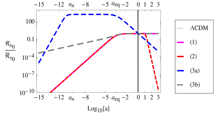
Figure 1: Evolution of ${\cal R}_{{s_{0}}}/\bar{\cal R}_{{s_{0}}}$ for the four cases described in table 2. The curves for $\Lambda$CDM and case (1) are overlapped.

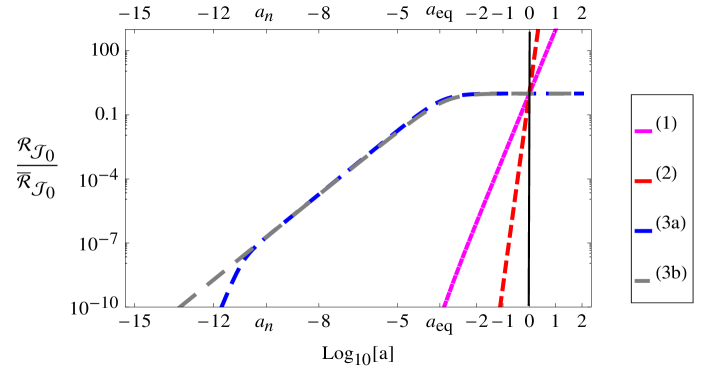
Figure 2: Evolution of the ratio ${\cal R}_{{\Im_{0}}}/\bar{\cal R}_{{\Im_{0}}}$ for the four cases described in table 2.

For case 1, we have taken $\Omega_{\Lambda}=1-\Omega_{r}-\Omega_{m}$ as in the $\Lambda$CDM case. For case 2, $\Omega_{\Lambda}=0.7498$ and $\Omega_{z}=1-\Omega_{r}-\Omega_{m}-\Omega_{\Lambda}=10^{-4}$. For 3$a$ we have set $\Omega_{z}=10^{-26}$ and $\Omega_{\Lambda}=1-\Omega_{r}-\Omega_{m}-\Omega_{z}$. Finally, for 3$b$ we have taken $\Omega_{z}=3\;10^{-4}$ and $\Omega_{\Lambda}=1-\Omega_{r}-\Omega_{m}-\Omega_{z}$.
Models 1 and 2 are characterised by an entropic active CC (potentials containing terms proportional to the combinations $b\;Y$) while for models 3 and 4 the DeSitter phase is induce by a sterile CC.

• The first model is characterised by a late time grow of the entropic perturbations, precisely from the period of DM-DE equality $a\sim(\Omega_{\Lambda}/\Omega_{m})^{1/3}$. Intrinsic pressure perturbations continue to growth also in the future as ${\cal R}\sim a^{3}\;\Im_{0}$ while the relative one are exactly the same of the $\Lambda$CDM model and flatten to ${\cal R}\sim s_{0}/3$.

• Also the second model is characterised by a late time fastest grow of the entropic perturbations. The intrinsic fluctuations grow as ${\cal R}\sim a^{9}\;\Im_{0}$ crossing the non perturbative regime in nearest future. The relative perturbations are exactly the same of the $\Lambda$CDM model but suddenly, in the future, will drop to zero as ${\cal R}\sim 1/a^{5}$.

• The model 3$a$ is characterised by the presence of a kineton phase ($w_{z}=1$) of the Universe in the very early time, before nucleosynthesis. In order to satisfy all the necessary constraints, the parameter $\Omega_{z}$ has to be extremely small $\sim 10^{-26}$. The intrinsic contribution grows until $a\sim(\Omega_{z}/\Omega_{r})^{1/2}$ and it “flattens” to ${\cal R}\sim a_{eq}\;\Im_{0}\;\Omega_{m}/\Omega_{z}$. Interestingly the relative contribution grows very fast as ${\cal R}\sim a^{2}\;\Omega_{m}/\Omega_{z}$ until $a\sim(\Omega_{z}/\Omega_{m})^{1/3}$, it flats at ${\cal R}\sim\frac{1}{a_{eq}}$ until equality time and then it decreases as ${\cal R}\sim a_{eq}/a$.

• Finally, model 3$b$ is characterised by the presence of a phase with $w_{z}=1/4$, intermediate to matter and radiation. The relative entropic contribution grows slowly up to equality time as ${\cal R}\sim a^{1/4}\;\Omega_{z}/\Omega_{r}$ and then it stays constant as in $\Lambda$CDM. The intrinsic corrections grow until equality time up to ${\cal R}\sim(\Omega_{m}/\Omega_{r})^{3/4}$ after they decrease as ${\cal R}\sim 1/a^{3/4}$.

The main impact of a non trivial entropic component in a dark fluid is the presence of a time dependent contribution to superhorizon scalar perturbations in the late time dynamics. In the above examples we tried to show a variety of possibilities. The above behaviours will impact mainly on the integrated Sachs-Wolfe effect (ISW) whose temperature fluctuations result from the differential redshift effect of photons climbing in and out of a time evolving potential perturbations from last scattering surface to the present day:

$$\left(\frac{\Delta T_{\gamma}}{T_{\gamma}}\right)_{(ISW)}=2\;\int^{\tau_{0}}_{\tau_{dec}}\,d\eta\;\partial_{\eta}\Phi(\eta,\;\vec{x}=\eta\;\vec{n})$$ (6.22)

with $\vec{n}^{2}=1$. When $\Phi$ is constant (from (4.16) imposing $\dot{\Phi}=0$ we get ${\cal R}=\frac{5+3\;w}{3\;(1+w)}\;\Phi$) the ISW effect is zero, as approximately it happens for adiabatic perturbations in $\Lambda$CDM model. It is clear from Figures (1) and (2) that the time behaviours of possible entropic seeds for cosmological perturbations have to be carefully estimated and included to check the stability of the $\Lambda$CDM predictions against possible modifications of paradigms.

7 Conclusions

In the present paper we have used the effective field theory description of perfect non-barotropic fluids showing that intrinsic entropic effects can be relevant. One of the major advantages of the field description is the fact that gives consistent non perturbative handle of the non-adiabatic part in the pressure variation. In addition one can also build a thermodynamical description of the fluid by relating field operators to basic thermodynamical variables. Then one can relate the non perturbative dynamics of vorticity and kinematical vorticity to the effective field theory approach. Such dynamics can be extracted from a Lagrangian whose structure is representing the free energy of the fluid. Inserting a metric in the Lagrangian formalism allows to directly obtain the red intertwined dynamical of gravity and of the fluid, together with its thermodynamical properties in the presence of gravity.
On the perturbative side one can develop the cosmological perturbations around FLRW spacetime. The effective description is very powerful and one can simply derive the evolution of the gravitational Bardeen potential, curvature perturbation ${\cal R}$ and uniform density surface curvature perturbation $\zeta$ setting the conditions for the violation of the Weinberg theorem. The entropy per particle perturbation $\delta\sigma$ is conserved and it acts just as a source term. On the more phenomenological side we have analysed the impact of a dark sector, taken as a single non-barotropic perfect fluid that mimics both DM and DE. In order to keep things simply enough to avoid numerical computations, we consider a set of two-fluid models composed by radiation and an interacting dark sector, neglecting baryons. Our results are compared against a simple version of $\Lambda$CDM model composed by two barotropic fluids (radiation plus dark matter) and a cosmological constant. From the field theory point of view, the presence of non trivial entropy emerges by the presence in the fluid Lagrangian $U$ of the operator $Y$ that can be identified with the dark sector temperature. The cosmological-like equation of state $w=-1$ can also be produced by a Lagrangian of the form $U(b\,Y)$. This means that a De Sitter phase can be obtained not only with a $\Lambda$ term but also with a peculiar non-barotropic fluid. Entropic perturbations, relative and intrinsic, are computed for a class of toy models that have very different temporal behaviour of perturbations triggered by entropic effects. Bounds on the scale of the corrections, proportional to $s_{0}$, for relative pressure perturbations, and to $\Im_{0}$ for intrinsic perturbations has to be settle by CMB [45] and large scale by the power spectrum [46]. In this work we showed how powerful can be the EFT formalism for the description of perfect fluid to study systematic way entropic effects and to simply recover known results on the non-perturbative dynamics of a fluid in the presence of gravity. For the models studied, we focused on the superhorizon evolution of the cosmological perturbations in presence of entropic fluid that can describe the yet unknown dark sector. Late time growing corrections to ${\cal R}$ are potentially at work (ISW effect) for quite general dark fluids that mimic dark matter and later dark energy. A numerical investigation to set the impact on Planck Data is necessary and it will given in a separate paper. It would be interesting to play a similar game during inflation/reheating.

Appendix A Single entropic fluid model as two barotropic fluids

It is interesting to investigate the behaviour of a simple single fluid model which reproduces the main features of the $\Lambda$CDM model. Take the following potential (without the radiation fluid of photons/neutrinos)

$$U=6\,H_{0}^{2}\,M_{\text{Pl}}^{2}\;\left(\frac{\Omega_{r}}{3}\;Y^{4}-\Omega_{m}\;b-\Omega_{\Lambda}\right)\,.$$ (A.1)

The sound speed $c_{s}^{2}$ and the equation of state $w$ are the same of $\Lambda$CDM and are given by (5.2). This it means that the background evolution from (A.1) and the $\Lambda$CDM model are the same. Being $c_{b}^{2}=1/3$ constant, from (3.6) the temperature of such a fluid scale as $T=Y=\frac{T_{0}}{a}\,,\;\phi^{\prime}=\varphi_{0}=\text{const.}$ The evolution of $T$ is typical of relativistic particles. The evolution of ${\cal R}$ is driven, at superhorizon scales, by intrinsic non-adiabatic perturbations (the relative entropic pressure is zero being the system composed by a single fluid) with

$$\Gamma_{\text{tot}}=\Gamma_{\text{int}}=\frac{\delta\sigma_{0}\,\varphi_{0}}{a^{3}\left(4\,a_{\text{eq}}+3\,a\right)}\,.$$ (A.2)

according to (4.19) we get

$${\cal R}=\frac{\,\delta\sigma_{0}\,\varphi_{0}}{8\,M_{\text{Pl}}^{2}\,H_{0}^{2}\,\Omega_{r}}\;\frac{a}{\left(3\,a+4\,a_{\text{eq}}\right)}\,.$$ (A.3)

Interestingly, the present single fluid model gives the very same evolution for superhorizon curvature perturbations as in $\Lambda$CDM, see (5.5), upon the following identification

$$({\rm in}\;\Lambda{\rm CDM})\;\;s_{0}\leftrightarrow-\frac{\delta\sigma_{0}\,\varphi_{0}}{8\,H_{0}^{2}\,M_{\text{Pl}}^{2}\,\Omega_{r}}\equiv\Im_{0}\,.$$ (A.4)

The dynamics of superhorizon perturbations of the single fluid model with Lagrangian (A.1) is the same of the $\Lambda$CDM model, however differences are present at small scales where for the $\Lambda$CDM model we have $v_{d}\neq 0$ while for the single fluid we have of course $v_{d}=0$.

The above result can be generalised to a single fluid described by

$$U=6\,M_{\text{Pl}}^{2}\,H_{0}^{2}\;\left[\,w_{r}\;\Omega_{r}\;Y^{(1+w_{r})/w_{r}}-\Omega_{m}\;b^{(1+w_{m})}-\Omega_{\Lambda}\,\right],$$ (A.5)

whose superhorizon perturbations are the same to the sum of two perfect barotropic fluids with equation state of state $w_{r}$ and $w_{m}$ respectively.

Appendix B Details of Case 3

The full expression for ${\cal R}$ in case 3$a$ of section 6.1 is

$${\cal R}=\frac{a\left[\Omega_{m}\,a^{3w_{z}}\left(\delta\sigma_{0}+6\,H_{0}^{2}\,M_{\text{Pl}}^{2}\,s_{0}\,\left(w_{z}+1\right)\Omega_{z}\right)+6\,H_{0}^{2}\,M_{\text{Pl}}^{2}\,s_{0}\left(w_{z}+1\right){}^{2}\,\Omega_{z}^{2}\right]}{6\,H_{0}^{2}M_{\text{Pl}}^{2}\left(w_{z}+1\right)\,\Omega_{z}\left[a^{3\,w_{z}}\left(3\,a\,\Omega_{m}+4\,\Omega_{r}\right)+3a\left(w_{z}+1\right)\Omega_{z}\right]}\,;$$ (B.1)

when $1/6<w_{z}<1/3$, while for $w_{z}>1/3$ we have (case 3$b$)

$${\cal R}=\frac{a^{3\,w_{z}}\left[a\,\delta\sigma_{0}\,\Omega_{m}-8\,H_{0}^{2}\,M_{\text{Pl}}^{2}\,s_{0}\,\Omega_{r}\left(w_{z}+1\right)\Omega_{z}\right]}{6\,H_{0}^{2}\,M_{\text{Pl}}^{2}\left(w_{z}+1\right)\Omega_{z}\left[a^{3\,w_{z}}\left(3\,a\,\Omega_{m}+4\,\Omega_{r}\right)+3a\left(w_{z}+1\right)\Omega_{z}\right]}\,.$$ (B.2)

References

- [1] Supernova Search Team collaboration, A. G. Riess et al., Observational evidence from supernovae for an accelerating universe and a cosmological constant, Astron. J. 116 (1998) 1009–1038, [astro-ph/9805201].
- [2] Supernova Cosmology Project collaboration, S. Perlmutter et al., Measurements of Omega and Lambda from 42 high redshift supernovae, Astrophys. J. 517 (1999) 565–586, [astro-ph/9812133].
- [3] DES collaboration, A. Drlica-Wagner et al., Dark Energy Survey Year 1 Results: Photometric Data Set for Cosmology, 1708.01531.
- [4] L. Amendola et al., Cosmology and Fundamental Physics with the Euclid Satellite, 1606.00180.
- [5] D. Spergel et al., Wide-Field InfrarRed Survey Telescope-Astrophysics Focused Telescope Assets WFIRST-AFTA 2015 Report, 1503.03757.
- [6] LSST Science, LSST Project collaboration, P. A. Abell et al., LSST Science Book, Version 2.0, 0912.0201.
- [7] G. Ballesteros, D. Comelli and L. Pilo, Massive and modified gravity as self-gravitating media, Phys. Rev. D94 (2016) 124023.
- [8] M. Celoria, D. Comelli and L. Pilo, Fluids, Superfluids and Supersolids: Dynamics and Cosmology of Self Gravitating Media, JCAP 1709 (2017) 036, [1704.00322].
- [9] H. Leutwyler, Nonrelativistic effective Lagrangians, Phys. Rev. D49 (1994) 3033–3043, [hep-ph/9311264].
- [10] H. Leutwyler, Phonons as goldstone bosons, Helv. Phys. Acta 70 (1997) 275–286, [hep-ph/9609466].
- [11] N. Arkani-Hamed, H. Georgi and M. Schwartz, Effective field theory for massive gravitons and gravity in theory space, Annals Phys. 305 (2003) 96–118, [hep-th/0210184].
- [12] V. A. Rubakov and P. G. Tinyakov, Infrared-modified gravities and massive gravitons, Phys. Usp. 51 (2008) 759–792, [0802.4379].
- [13] S. L. Dubovsky, Phases of massive gravity, JHEP 10 (2004) 076, [hep-th/0409124].
- [14] S. Dubovsky, T. Gregoire, A. Nicolis and R. Rattazzi, Null energy condition and superluminal propagation, JHEP 03 (2006) 025, [hep-th/0512260].
- [15] S. Dubovsky, L. Hui, A. Nicolis and D. Son, Effective field theory for hydrodynamics: thermodynamics, and the derivative expansion, Phys. Rev. D85 (2012) 085029, [1107.0731].
- [16] A. Nicolis, Low-energy effective field theory for finite-temperature relativistic superfluids, 1108.2513.
- [17] G. Ballesteros and B. Bellazzini, Effective perfect fluids in cosmology, JCAP 1304 (2013) 001, [1210.1561].
- [18] S. Weinberg, Adiabatic modes in cosmology, Phys. Rev. D67 (2003) 123504, [astro-ph/0302326].
- [19] S. Weinberg, Cosmology, Oxford Univ. Press (2008) .
- [20] G. F. R. Ellis, J. Hwang and M. Bruni, Covariant and Gauge Independent Perfect Fluid Robertson-Walker Perturbations, Phys. Rev. D40 (1989) 1819–1826.
- [21] G. F. R. Ellis, M. Bruni and J. Hwang, Density Gradient - Vorticity Relation in Perfect Fluid Robertson-Walker Perturbations, Phys. Rev. D42 (1990) 1035–1046.
- [22] G. Ballesteros, D. Comelli and L. Pilo, Thermodynamics of perfect fluids from scalar field theory, Phys. Rev. D94 (2016) 025034.
- [23] H. Kodama and M. Sasaki, Cosmological Perturbation Theory, Prog. Theor. Phys. Suppl. 78 (1984) 1.
- [24] D. Langlois and F. Vernizzi, Evolution of non-linear cosmological perturbations, Phys. Rev. Lett. 95 (2005) 091303, [astro-ph/0503416].
- [25] D. Langlois and F. Vernizzi, Conserved non-linear quantities in cosmology, Phys. Rev. D72 (2005) 103501, [astro-ph/0509078].
- [26] A. Lichnerowicz, Relativistic Hydrodynamics and Magnetohydrodynamics. Benjamin New York, 1967.
- [27] B. Carter, Covariant Theory of Conductivity in Ideal Fluid or Solid Media, Lect. Notes Math. 1385 (1989) 1–64.
- [28] A. J. Christopherson, K. A. Malik and D. R. Matravers, Vorticity generation at second order in cosmological perturbation theory, Phys. Rev. D79 (2009) 123523, [0904.0940].
- [29] I. A. Brown, A. J. Christopherson and K. A. Malik, The magnitude of the non-adiabatic pressure in the cosmic fluid, Mon. Not. Roy. Astron. Soc. 423 (2012) 1411–1415, [1108.0639].
- [30] A. J. Christopherson, The future of cosmology and the role of non-linear perturbations, Commun. Theor. Phys. 57 (2012) 323–325, [1111.6853].
- [31] A. J. Christopherson, Cosmological Perturbations: Vorticity, Isocurvature and Magnetic Fields, Int. J. Mod. Phys. D23 (2014) 1430024, [1409.4721].
- [32] A. R. Liddle and D. H. Lyth, The Cold dark matter density perturbation, Phys. Rept. 231 (1993) 1, [astro-ph/9303019].
- [33] D. H. Lyth and A. Riotto, Particle physics models of inflation and the cosmological density perturbation, Phys. Rept. 314 (1999) 1, [hep-ph/9807278].
- [34] J. M. Bardeen, P. J. Steinhardt and M. S. Turner, Spontaneous Creation of Almost Scale - Free Density Perturbations in an Inflationary Universe, Phys. Rev. D28 (1983) 679.
- [35] D. Wands, K. A. Malik, D. H. Lyth and A. R. Liddle, A New approach to the evolution of cosmological perturbations on large scales, Phys. Rev. D62 (2000) 043527.
- [36] W. H. Kinney, Horizon crossing and inflation with large eta, Phys. Rev. D72 (2005) 023515, [gr-qc/0503017].
- [37] M. H. Namjoo, H. Firouzjahi and M. Sasaki, Violation of non-Gaussianity consistency relation in a single field inflationary model, Europhys. Lett. 101 (2013) 39001, [1210.3692].
- [38] H. Motohashi, A. A. Starobinsky and J. Yokoyama, Inflation with a constant rate of roll, JCAP 1509 (2015) 018, [1411.5021].
- [39] M. Akhshik, H. Firouzjahi and S. Jazayeri, Effective Field Theory of non-Attractor Inflation, JCAP 1507 (2015) 048, [1501.01099].
- [40] M. Akhshik, R. E. H. Firouzjahi and Y. Wang, Statistical Anisotropies in Gravitational Waves in Solid Inflation, JCAP 1409 (2014) 012, [1405.4179].
- [41] K. A. Malik, D. Wands and C. Ungarelli, Large scale curvature and entropy perturbations for multiple interacting fluids, Phys. Rev. D67 (2003) 063516, [astro-ph/0211602].
- [42] Planck collaboration, P. A. R. Ade et al., Planck 2015 results. XIII. Cosmological parameters, Astron. Astrophys. 594 (2016) A13, [1502.01589].
- [43] Planck collaboration, P. A. R. Ade et al., Planck 2015 results. XX. Constraints on inflation, Astron. Astrophys. 594 (2016) A20, [1502.02114].
- [44] J. A. S. Lima and J. S. Alcaniz, Thermodynamics and spectral distribution of dark energy, Phys. Lett. B600 (2004) 191, [astro-ph/0402265].
- [45] D. Langlois and B. van Tent, Isocurvature modes in the CMB bispectrum, JCAP 1207 (2012) 040, [1204.5042].
- [46] D. Langlois and A. Riazuelo, Correlated mixtures of adiabatic and isocurvature cosmological perturbations, Phys. Rev. D62 (2000) 043504, [astro-ph/9912497].