Including particle-vibration coupling in the Fayans functional. Odd-even mass differences of semi-magic nuclei.

Abstract

A method to evaluate the particle-phonon coupling (PC) corrections to the single-particle energies in semi-magic nuclei, based on the direct solution of the Dyson equation with PC corrected mass operator, is presented. It is used for finding the odd-even mass difference between even Pb and Sn isotopes and their odd-proton neighbors. The Fayans energy density functional (EDF) DF3-a is used which gives rather highly accurate predictions for these mass differences already at the mean-field level. In the case of the lead chain, account for the PC corrections induced by the low-laying phonons $2^{+}_{1}$ and $3^{-}_{1}$ makes agreement of the theory with the experimental data significantly better. For the tin chain, the situation is not so definite. In this case, the PC corrections make agreement better in the case of the addition mode but they spoil the agreement for the removal mode. We discuss the reason of such a discrepancy.

I Introduction

Ability to describe nuclear single-particle (SP) spectra correctly is an important feature of any self-consistent nuclear theory. Last decade is characterized with a revival of the interest to study the particle-phonon coupling (PC) corrections to the SP spectra within different self-consistent nuclear approaches. Up to now, they were limited only to magic nuclei, see a study of this problem within the relativistic mean-field theory Litv-Ring , and several ones within the Skyrme–Hartree–Fock method Bort ; Dobaczewski ; Baldo-PC . The consideration of this problem levels on the basis of the self-consistent theory of finite Fermi systems (TFFS) scTFFS differs from those cited above by the account for the non-pole terms of the PC correction $\delta\Sigma^{\rm PC}$ to the mass operator $\Sigma_{0}$. In the nuclear PC problem, the non-pole diagrams of the operator $\delta\Sigma^{\rm PC}$ were considered firstly by Khodel Khod-76 , see also scTFFS . These diagrams are also sometimes named “the phonon tadpole” phon-tad , by the analogy with the tadpole-like diagrams in field theory tad .

There are several reasons, why the magic nuclei were chosen as a polygon for studying the PC corrections to SP levels. First, the experimental SP levels are known in detail only for magic nuclei lev-exp . Second, these nuclei are non-superfluid, which makes the formulas for the PC correction $\delta\Sigma^{\rm PC}$ to the mass operator much simpler than their analogue in the superfluid case phon-tad . At last, in these nuclei, the PC strength is rather week and the perturbation theory in $g_{L}^{2}$ is valid, $g_{L}$ being the creation vertex of the $L$-phonon. Moreover, the perturbation theory in $\delta\Sigma^{\rm PC}$ can be used for solving the Dyson equation with the mass operator $\Sigma^{\rm PC}(\varepsilon){=}\Sigma_{0}{+}\delta\Sigma^{\rm PC}(\varepsilon)$.

Another situation occurs often in semi-magic nuclei lev-semi , due to a strong mixture of some SP states $|\lambda\rangle$ with those possessing the structure of ($|\lambda\rangle$ + $L$-phonon). For such cases a method was used in lev-semi based on the direct solution of the Dyson equation with the mass operator $\Sigma^{\rm PC}(\varepsilon)$. Such a method was developed by Ring and Werner in 1973 Ring-Werner . As result of such solution each SP state $|\lambda\rangle$ splits to a set of $|\lambda,i\rangle$ solutions with the SP strength distribution factors $S^{i}_{\lambda}$. An approximate expression for the non-pole term of $\delta\Sigma^{\rm PC}$ was used in lev-semi , just as in levels , which is valid for heavy nuclei.

A method was proposed, how to express the average SP energy $\varepsilon_{\lambda}$ and the average $Z_{\lambda}$ factor in terms of $\varepsilon_{\lambda}^{i}$ and $S_{\lambda}^{i}$. It is similar to the one used usually for finding the corresponding experimental values lev-exp . Unfortunately, the experimental data in heavy non-magic nuclei considered in lev-semi are practically absent. However, there is a massive set of data which has a direct relevance to the solutions $\varepsilon_{\lambda}^{i}$ under discussion, namely, the odd-even mass differences, that is the “chemical potentials” in terms of the TFFS AB . This quantity was analyzed in in a brief letter chim-pots for the lead chain. In this article, we present a detailed analysis of these results and carry out the analogous calculations for the tin chain.

II Direct solution of the Dyson equation with PC corrected mass operator

In this article, just as in Refs. levels ; lev-semi ; chim-pots , we use the self-consistent basis generated with the energy density functional (EDF) by Fayans Fay1 ; Fay4 ; Fay :

$$E_{0}=\int d^{3}r{\cal E}\left(\rho({\bf r}),\nu({\bf r)}\right),$$ (1)

which depends on the equal footing on the normal density $\rho$ and the anomalous one $\nu$. Note, that from the very beginning Fayans with the coauthors supposed that the parameters of the EDF should be chosen in such a way that they take into account various PC corrections on average.

To find the SP energies with account for the PC effects, we solve the following equation:

$$\left(\varepsilon-H_{0}-\delta\Sigma^{\rm PC}(\varepsilon)\right)\phi=0,$$ (2)

where $H_{0}$ is the quasiparticle Hamiltonian with the spectrum $\varepsilon_{\lambda}^{(0)}$ and $\delta\Sigma^{\rm PC}$ is the PC correction to the quasiparticle mass operator. This is equivalent to the Dyson equation for the one-particle Green function $G$ with the mass operator $\Sigma(\varepsilon)=\Sigma_{0}+\delta\Sigma^{\rm PC}(\varepsilon)$.

For brevity, we present below explicit formulas for one $L$-phonon. In the case when several $L$-phonons are taken into account, the total PC variation of the mass operator in Eq. (2) is the sum over all phonons:

$$\delta\Sigma^{\rm PC}=\sum_{L}\delta\Sigma^{\rm PC}_{L}.$$ (3)

The corresponding diagrams for the PC correction $\delta\Sigma^{\rm PC}_{L}$ to the mass operator $\Sigma_{0}$, in the representation of the SP states $|\lambda\rangle$, are displayed in Fig. 1. The first one is the usual pole diagram, with obvious notation, whereas the second one represents the sum of all non-pole diagrams of the order $g_{L}^{2}$.

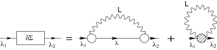
Figure 1: PC corrections to the mass operator. The open circle is the vertex $g_{L}$ of the $L$-phonon creation. The gray blob denotes the phonon non-pole (“tadpole”) term.

In magic nuclei, the vertex $g_{L}$ in Fig. 1 obeys the RPA-like TFFS equation AB

$${g_{L}}(\omega)={{\cal F}}{A}(\omega){g_{L}}(\omega),$$ (4)

where $A(\omega)=\int G\left(\varepsilon+\omega/2\right)G\left(\varepsilon-\omega/2\right)d\varepsilon/(2\pi i)$ is the particle-hole propagator and ${\cal F}$ is the Landau-Migdal (LM) interaction amplitude.

The expression for the pole term in magic nuclei is well known Litv-Ring ; Bort ; levels , but we present it here for completeness. In obvious symbolic notation, the pole diagram corresponds to $\delta\Sigma^{\rm pole}_{L}=(g_{L},D_{L}Gg_{L})$, where $D_{L}(\omega)$ is the $L$-phonon $D$-function:

$$D_{L}(\omega)=\frac{1}{\omega-\omega_{L}+i\gamma}-\frac{1}{\omega+\omega_{L}-i\gamma}\,,$$ (5)

where $\omega_{L}$ is the $L$-phonon excitation energy.

Explicitly, one obtains

$$\delta\Sigma^{\rm pole}_{\lambda_{1}\lambda_{2}}(\epsilon) = \sum_{\lambda\,M}\langle\lambda_{1}|g_{LM}|\lambda\rangle\langle\lambda|g^{+}_{LM}|\lambda_{2}\rangle$$ (6)

$$\times \left(\frac{n_{\lambda}}{\varepsilon+\omega_{L}-\varepsilon_{\lambda}^{(0)}}+\frac{1-n_{\lambda}}{\varepsilon-\omega_{L}-\varepsilon_{\lambda}^{(0)}}\right),$$

where $n_{\lambda}=(0,1)$ stands for the occupation numbers.

As to the non-pole term, we follow to the method developed by Khodel Khod-76 , see also scTFFS . The second, non-pole, term in Fig. 1 is

$$\delta\Sigma^{\rm non-pole}=\int\frac{d\omega}{2\pi i}\delta_{L}{g_{L}}D_{L}(\omega),$$ (7)

where $\delta_{L}{g_{L}}$ can be found by variation of Eq. (4) in the field of the $L$-phonon:

$$\delta_{L}{g_{L}} = \delta_{L}{\cal F}A(\omega_{L}){g_{L}}+{\cal F}\delta_{L}A(\omega_{L}){g_{L}}$$ (8)

$$+ {\cal F}A(\omega_{L})\delta_{L}{g_{L}}.$$

All the low-lying phonons we deal with are of surface nature, the surface peak dominating in their creation amplitude:

$$g_{L}(r)=\alpha_{L}\frac{dU}{dr}+\chi_{L}(r).$$ (9)

The first term in this expression is surface peaked, whereas the in-volume addendum $\chi_{L}(r)$ is rather small. It is illustrated in Fig. 2 for the $2^{+}_{1}$ and $3^{-}_{1}$ states in ²⁰⁴Pb. If one neglects this in-volume term $\chi_{L}$, very simple expression for the non-pole term can be obtained scTFFS :

$$\delta\Sigma^{\rm non-pole}_{L}=\frac{\alpha_{L}^{2}}{2}\frac{2L+1}{3}\triangle U(r).$$ (10)

Just as in levels ; lev-semi , below we will neglect the in-volume term in (9) and use Eq. (10) for the non-pole term of $\delta\Sigma_{L}^{\rm PC}$.

All the low-lying phonons we consider have natural parity. In this case, the vertex $g_{L}$ possesses even $T$-parity. It is a sum of two components with spins $S=0$ and $S=1$, respectively,

$$g_{L}=g_{L0}(r)T_{LL0}({\bf n,\alpha})+g_{L1}(r)T_{LL1}({\bf n,\alpha}),$$ (11)

where $T_{JLS}$ stand for the usual spin-angular tensor operators BM1 . The operators $T_{LL0}$ and $T_{LL1}$ have opposite $T$-parities, hence the spin component should be the odd function of the excitation energy, $g_{L1}\propto\omega_{L}$. In all the cases we consider the component $g_{L1}$ is negligible and the component $g_{L0}$ only will be retained, the index ’0’ being for brevity omitted: $g_{L0}\to g_{L}$.

As it was discussed in the introduction, any semi-magic nucleus consists of two sub-systems with absolutely different properties, the normal and superfluid ones. Following to lev-semi , we consider the SP spectra only of the normal subsystem, e.g. the proton spectra for the lead isotopes. In this case, all the above formulas remain valid with one exception. Now the vertex $g_{L}(\bf r)$ obeys the QRPA-like TFFS equation AB ,

$${\hat{g}}_{L}(\omega)={\hat{\cal F}}{\hat{A}}(\omega){\hat{g}}_{L}(\omega),$$ (12)

where all the terms are matrices. The angular momentum projection $M$, which is written down in Eq. (6) explicitly, is here and below for brevity omitted. In the standard TFFS notation, we have:

$${\hat{g}}_{L}=\left(\begin{array}[]{c}g_{L}^{(0)}\\ g_{L}^{(1)}\\ g_{L}^{(2)}\end{array}\right),$$ (13)

$${\hat{\cal F}}=\left(\begin{array}[]{ccc}{\cal F}&{\cal F}^{\omega\xi}&{\cal F}^{\omega\xi}\\ {\cal F}^{\xi\omega}&{\cal F}^{\xi}&{\cal F}^{\xi\omega}\\ {\cal F}^{\xi\omega}&{\cal F}^{\xi\omega}&{\cal F}^{\xi}\end{array}\right).$$ (14)

In (13), $g^{(0)}$ is the normal component of the vertex ${\hat{g}}$, whereas $g^{(1),(2)}$ are two anomalous ones. In Eq. (14), $\cal{F}$ is the usual LM interaction amplitude which is the second variation derivative of the EDF ${\cal E}[\rho,\nu]$ over the normal density $\rho$ . The effective pairing interaction $\cal{F}^{\xi}$ is the second derivative of the EDF over the anomalous density $\nu$. At last, the amplitude ${\cal F}^{\xi\omega}$ stands for the mixed derivative of ${\cal E}$ over $\rho$ and $\nu$.

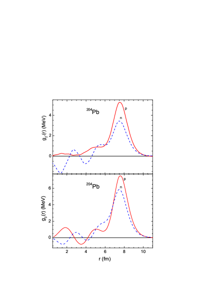
Figure 2: (Color online) Phonon creation amplitudes $g_{L}(r)$ for two low-lying phonons in the ²⁰⁴Pb nucleus.

The matrix ${\hat{A}}$ consists of $3\times 3$ integrals over $\varepsilon$ of the products of different combinations of the Green function $G(\varepsilon)$ and two Gor’kov functions $F^{(1)}(\varepsilon)$ and $F^{(2)}(\varepsilon)$ AB .

As we need the proton vertex ${\hat{g}}_{L}^{p}$ and the proton subsystem is normal, only the normal vertex $g_{L}^{(0)p}$ is non-zero in this case. This is the meaning of the abbreviated notation $g_{L}$ in (6) and below.

For solving the above equations, we use the self-consistent basis generated by the version DF3-a DF3-a of the Fayans EDF DF3 Fay4 ; Fay . The nuclear mean-field potential $U(r)$ is the first derivative of ${\cal E}$ in (1) over $\rho$.

In magic nuclei levels , the perturbation theory in $\delta\Sigma^{\rm PC}$ with respect to $H_{0}$ can be used to solve this equation:

$$\varepsilon_{\lambda}=\varepsilon_{\lambda}^{(0)}+Z_{\lambda}^{\rm PC}\delta\Sigma^{\rm PC}_{\lambda\lambda}(\varepsilon_{\lambda}^{(0)}),$$ (15)

where

$$Z_{\lambda}^{\rm PC}=\left({1-\left(\frac{\partial}{\partial\varepsilon}\delta\Sigma^{\rm PC}(\varepsilon)\right)_{\varepsilon=\varepsilon_{\lambda}^{(0)}}}\right)^{-1}.$$ (16)

Another situation is typical for semi-magic nuclei, where small denominators $\varepsilon^{(0)}_{1}-\varepsilon^{(0)}_{2}\pm\omega_{L}$ can appear in Eq. (6). We demonstrate in Table I the poor applicability of the perturbation theory on the example of the ²⁰⁴Pb nucleus with the use of two phonons, $2_{1}^{+},\omega_{2}{=}0.88\;$MeV and $3_{1}^{-},\omega_{3}{=}2.79\;$MeV. The value of $\delta\varepsilon_{\lambda}^{\rm PC}$ in the column 6 is found as a sum of the values in three previous columns multiplied, in accordance with Eq. (15), by the total $Z$-factor in the last column.

The most dangerous denominator is now $\varepsilon^{(0)}(2d_{3/2}){-}\varepsilon^{(0)}(3s_{1/2}){+}\omega_{2}{=}0.09\;$MeV. The state 2$d_{3/2}$ is an obvious victim of the use of a non-adequate perturbation theory in this case. Indeed, the inequality $1{-}Z_{\lambda}^{\rm PC}<<1$ is a necessary condition for applicability of the perturbation theory. For the 2$d_{3/2}$ state, we have the value of 0.95 for the left hand side of this inequality, which is almost equal to unit. In the table, there are other examples of poor applicability of the perturbation theory, but they are not so demonstrative.

Table 1: PC corrected proton SP energies $\varepsilon_{\lambda}$ and $Z$-factors of ²⁰⁴Pb nucleus found from the perturbation theory prescription (15) and (16).

$\lambda$	$\varepsilon^{(0)}_{\lambda}$	$\delta\Sigma_{\lambda\lambda}^{\rm pole}$	$\delta\Sigma_{\lambda\lambda}^{\rm non-pole}$	’ghost’	$\delta\varepsilon_{\lambda}^{\rm PC}$	$\varepsilon_{\lambda}^{\rm PC}$	$Z_{\lambda}^{\rm PC}(L{=}2)$	$Z_{\lambda}^{\rm PC}(L{=}3)$	$Z_{\lambda}^{\rm PC}$
1$i_{13/2}$	-1.21	-1.01	0.32	0.04	-0.37	-1.58	0.64	0.82	0.56
2$f_{7/2}$	-2.01	-0.81	0.20	0.03	-0.36	-2.37	0.66	0.90	0.62
1$h_{9/2}$	-3.36	-0.43	0.27	0.04	-0.09	-3.45	0.74	0.98	0.73
3$s_{1/2}$	-6.72	0.07	0.17	0.03	0.22	-6.50	0.84	0.96	0.82
2$d_{3/2}$	-7.51	2.02	0.17	0.03	0.10	-7.40	0.05	0.97	0.05
1$h_{11/2}$	-7.98	0.28	0.30	0.04	0.42	-7.56	0.70	0.96	0.68
2$d_{5/2}$	-8.80	0.33	0.18	0.03	0.26	-8.541	0.57	0.80	0.50
1$g_{7/2}$	-10.93	-0.23	0.24	0.03	0.01	-10.92	0.79	0.35	0.32

For such cases, a method based on the direct solution of the Dyson equation (2) was developed in lev-semi . We describe it with the example of the same nucleus ²⁰⁴Pb which was considered above to demonstrate the non-applicability of the perturbation theory. The model was suggested based on the fact that the PC corrections are important only for the SP levels nearby the Fermi surface. A model space $S_{0}$ was considered including two shells close to it, i.e. one hole and one particle shells. To avoid any misunderstanding, we stress that this restriction concerns only Eq. (2). In Eq. (6) for $\delta\Sigma^{\rm pole}$, we use rather wide SP space with energies $\varepsilon_{\lambda}^{(0)}{<}40\;$MeV. The space $S_{0}$ involves 5 hole states (1g_7/2, 2d_5/2, 1h_11/2, 2d_3/2, 3s_1/2) and four particle ones (1g_9/2, 2f_7/2, 1i_13/2, 2f_5/2). We see that there is here only one state for each $(l,j)$ value. Therefore, we need only diagonal elements $\delta\Sigma^{\rm pole}_{\lambda\lambda}$ in (6), which simplifies very much the solution of the Dyson equation. As a consequence, Eq. (2) reduces as follows:

$$\varepsilon-\varepsilon_{\lambda}^{(0)}-\delta\Sigma^{\rm PC}_{\lambda\lambda}(\varepsilon)=0.$$ (17)

The non-pole term does not depend on the energy, therefore only poles of Eq. (6) are the singular points of Eq. (17). They can be readily found from (6) in terms of $\varepsilon_{\lambda}^{(0)}$ and $\omega_{L}$. It can be easily seen that the l.h.s of Eq. (17) always changes sign between any couple of neighboring poles, and the corresponding solution $\varepsilon_{\lambda}^{i}$ can be found with usual methods. In this notation, $\lambda$ is just the index for the initial single-particle state from which the state $|\lambda,i\rangle$ originated. The latter is a mixture of a single-particle state with several particle-phonon states. The corresponding single-particle strength distribution factors ($S$-factors) can be found similar to (16):

$$S_{\lambda}^{i}=\left(1-\left(\frac{\partial}{\partial\varepsilon}\delta\Sigma^{\rm PC}(\varepsilon)\right)_{\varepsilon=\varepsilon_{\lambda}^{i}}\right)^{-1}.$$ (18)

Evidently, they should obey the normalization rule:

$$\sum_{i}S_{\lambda}^{i}=1.$$ (19)

The accuracy of fulfillment of this relation is a measure of validity of the model space $S_{0}$ we use to solve the problem under consideration.

Table 2: Examples of solutions of Eq. (17) for protons in ²⁰⁴Pb.

$\lambda$	$i$	$\varepsilon_{\lambda}^{i}$	$S_{\lambda}^{i}$
1$h_{9/2}$	1	-13.736	0.220 $\times 10^{-2}$
	2	-11.596	0.777 $\times 10^{-3}$
	3	-10.339	0.674 $\times 10^{-2}$
	4	-8.862	0.484 $\times 10^{-3}$
	5	-3.447	0.760
	6	-2.217	0.199
	7	-1.122	0.288 $\times 10^{-2}$
			$\sum S_{\lambda}^{i}{=}0.987$
3$s_{1/2}$	1	-9.877	0.608 $\times 10^{-1}$
	2	-8.536	0.604 $\times 10^{-1}$
	3	-6.493	0.839
			$\sum S_{\lambda}^{i}{=}0.990$
1$h_{11/2}$	1	-13.717	0.692 $\times 10^{-3}$
	2	-11.690	0.256 $\times 10^{-1}$
	3	-9.084	0.134
	4	-7.509	0.814
	5	-2.471	0.427 $\times 10^{-3}$
	6	-1.095	0.473 $\times 10^{-2}$
			$\sum S_{\lambda}^{i}{=}0.985$
2$d_{5/2}$	1	-11.817	0.314 $\times 10^{-2}$
	2	-11.150	0.139
	3	-9.799	0.516 $\times 10^{-1}$
	4	-8.580	0.312
	5	-8.195	0.295
	6	-7.404	0.171
	7	-0.564	0.791 $\times 10^{-3}$
			$\sum S_{\lambda}^{i}{=}0.978$

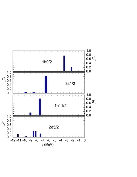
Figure 3: (Color online) The SP strengh distributions ($S$-factors) of four states in the ²⁰⁴Pb nucleus.

A set of solutions for four $|\lambda,i\rangle$ states in the ²⁰⁴Pb nucleus is presented in Table II. The corresponding $S$-factors are displayed in Fig. 3. In three upper cases for a given $\lambda$ there is a state $|\lambda,i_{0}\rangle$ with dominating $S_{\lambda}^{i_{0}}$ value (${\simeq}0.8$). They are examples of “good” single-particle states. In such cases, the following prescription looks natural for the PC corrected single-particle characteristics:

$$\varepsilon_{\lambda}={\varepsilon}_{\lambda}^{i_{0}};\;Z_{\lambda}^{\rm PC}=S_{\lambda}^{i_{0}}.$$ (20)

These are the analogous to Eqs. (15) and (16) in the perturbative solution.

The lowest panel in Fig. 3 represents a case of a strong spread where there are two or more numbers $i$ with comparable values of the spectroscopic factors $S_{\lambda}^{i}$. For such cases, the following generalization of Eq. (20) was suggested in lev-semi :

$$\varepsilon_{\lambda}=\frac{1}{Z_{\lambda}^{\rm PC}}\sum_{i}{\varepsilon}_{\lambda}^{i}S_{\lambda}^{i},$$ (21)

where

$$Z_{\lambda}^{\rm PC}=\sum_{i}S_{\lambda}^{i}.$$ (22)

The average SP energies and the $Z$-factors found according to the above prescriptions are presented in Table III.

Table 3: PC corrected proton single-particle characteristics $\varepsilon_{\lambda}$ and $Z_{\lambda}$ of ²⁰⁴Pb nucleus found with Eqs. (20) or (21) and (22). The total correction to the SPE $\delta\varepsilon_{\lambda}^{\rm PC}{=}\varepsilon_{\lambda}{-}\varepsilon_{\lambda}^{(0)}$ is presented.

$\lambda$	$\varepsilon^{(0)}_{\lambda}$	$\delta\varepsilon_{\lambda}^{\rm PC}$	$\varepsilon_{\lambda}$	$Z_{\lambda}$
1$i_{13/2}$	-1.21	0.14	-1.07	0.97
2$f_{7/2}$	-2.01	-0.23	-2.24	0.87
1$h_{9/2}$	-3.36	0.17	-3.19	0.96
3$s_{1/2}$	-6.72	0.23	-6.49	0.84
2$d_{3/2}$	-7.51	0.05	-7.46	0.94
1$h_{11/2}$	-7.98	0.25	-7.73	0.95
2$d_{5/2}$	-8.80	0.17	-8.63	0.92
1$g_{7/2}$	-10.93	0.13	-10.80	0.95

Comparison of Table III with the perturbation theory Table I shows limited common features. In particular, the state 2$d_{3/2}$ is now absolutely “healed” with a big value of the $Z$-factor and a small shift of the PC corrected energy from the initial value.

III PC corrections to the odd-even mass differences of semi-magic nuclei

As it was discussed in Introduction, in heavy semi-magic nuclei the experimental data on the SP energies are practically absent, but there is another kind of observables, the odd-even mass differences, which has a direct relevance to the set of the solutions $\varepsilon_{\lambda}^{i}$ of the Dyson equation in the form (17). In terms of the (TFFS) AB they are named “chemical potentials”:

$$\mu_{+}^{n}(Z,N)=-\left(B(Z,N+1)-B(Z,N)\right),$$ (23)

$$\mu_{-}^{n}(Z,N)=-\left(B(Z,N)-B(Z,N-1)\right).$$ (24)

$$\mu_{+}^{p}(Z,N)=-\left(B(Z+1,N)-B(Z,N)\right),$$ (25)

$$\mu_{-}^{p}(Z,N)=-\left(B(Z,N)-B(Z-1,N)\right),$$ (26)

where $B(Z,N)$ is the binding energy of the corresponding nucleus. Evidently, they are equal to one nucleon separation energies $S_{n,p}$ BM1 taken with the opposite sign. For example, we have $\mu_{-}^{n}(Z,N){=}{-}S_{n}(Z,N)$ or $\mu_{+}^{n}(Z,N){=}{-}S_{n}(Z,N+1)$.

Table 4: Excitation energies $\omega_{L}$ (MeV) and the coefficients $\alpha_{L}$ (fm) in Eq. (9) of the $2^{+}_{1}$ and $3^{-}_{1}$ phonons in even Pb isotopes.

A	$\omega_{2}$	$\omega_{2}^{\rm exp}$	$\alpha_{2}$	$\omega_{3}$	$\omega_{3}^{\rm exp}$	$\alpha_{3}$
180	1.415	1.168(1)	0.31	2.008	–	0.35
182	1.284	0.888	0.31	1.836	–	0.35
184	1.231	0.702	0.32	1.839	–	0.36
186	1.133	0.662	0.33	1.881	–	0.34
188	1.028	0.724	0.34	1.968	–	0.34
190	0.930	0.774	0.36	2.052	–	0.33
192	0.849	0.854	0.35	2.160	–	0.32
194	0.792	0.965	0.35	2.272	–	0.32
196	0.764	1.049	0.35	2.390	2.471(?)	0.31
198	0.762	1.064	0.35	2.506	–	0.31
200	0.789	1.027	0.30	2.620	–	0.31
202	0.823	0.961	0.31	2.704	2.517	0.31
204	0.882	0.899	0.22	2.785	2.621	0.31
206	0.945	0.803	0.16	2.839	2.648	0.32
208	4.747	4.086	0.33	2.684	2.615	0.09
210	1.346	0.800	0.07	2.183	1.870(10)	0.19
				2.587	2.828(10)	0.17
212	1.444	0.805	0.17	1.788	1.820(10)	0.36
214	1.125	0.835(1)	0.19	1.469	–	0.37

Indeed, let us write down the Lehmann spectral expansion for the Green function $G(\varepsilon;{\bf r_{1}},{\bf r_{2}})$ in the $\lambda$-representation of the functions which diagonalize $G$ AB :

$$G_{\lambda}(\varepsilon){=}\sum_{s}\frac{|(a^{+}_{\lambda})_{s0}|^{2}}{\varepsilon{-}(E_{s}{-}E_{0}){+}i\gamma}{+}\sum_{s}\frac{|(a_{\lambda})_{s0}|^{2}}{\varepsilon{+}(E_{s}{-}E_{0}){-}i\gamma},$$ (27)

with obvious notation. The isotopic index $\tau=(n,p)$ in (27) is for brevity omitted. In both the sums, the summation is carried out for the exact states $|s\rangle$ of nuclei with one added or removed nucleon. Explicitly, if $|0\rangle$ is the ground state of the even-even ($Z,N$) nucleus, the states $|s\rangle$ in the first sum correspond to the ($Z,N+1$) one for $\tau=n$ and ($Z+1,N$) for $\tau=p$. Correspondingly, in the second sum they are ($Z,N-1$) for $\tau=n$ and (Z-1,$N$) for $\tau=p$. If $|s\rangle$ is a ground state of the corresponding odd nucleus, the corresponding pole in (27) coincides with one the chemical potentials (23) – (26). At the mean field level, they can be attributed to the SP energies $\varepsilon_{\lambda}$ with zero excitation energy, whereas with account for the PC corrections they should coincide with the corresponding energies $\varepsilon_{\lambda}^{i}$.

Table 5: Proton odd-even mass differences $\mu_{+}$ (MeV) for the even Pb isotopes. The mean field predictions for the Fayans EDF DF3-a and those with the PC corrections are given.

nucl.	$\lambda$	DF3-a	DF3-a + $2^{+}$	DF3-a + $(2^{+}{+}3^{-})$	exp mass
180Pb	1$h_{9/2}$	3.513	3.185	3.321	—
182Pb	1$h_{9/2}$	2.942	2.564	2.695	—
184Pb	$1h_{9/2}$	2.360	1.906	2.093	1.527(0.094)
186Pb	$1h_{9/2}$	1.767	1.293	1.441	1.010(0.021)
188Pb	$1h_{9/2}$	1.172	0.683	0.806	0.461(0.031)
190Pb	$1h_{9/2}$	0.577	0.027	0.141	-0.112(0.020)
192Pb	$1h_{9/2}$	-0.017	-0.528	-0.420	-0.596(0.022)
194Pb	$1h_{9/2}$	-0.608	-1.167	-1.058	-1.107(0.023)
196Pb	$1h_{9/2}$	-1.193	-1.760	-1.658	-1.615(0.023)
198Pb	$1h_{9/2}$	-1.769	-2.316	-2.212	-2.036(0.025)
200Pb	$1h_{9/2}$	-2.327	-2.757	-2.648	-2.453(0.026)
202Pb	$1h_{9/2}$	-5.806	-5.177	-5.317	-5.480(0.039)
204Pb	$1h_{9/2}$	-3.356	-3.567	-3.447	-3.244(0.006)
206Pb	$1h_{9/2}$	-3.818	-3.911	-3.771	-3.558(0.004)
208Pb	$1h_{9/2}$	-4.232	-4.064	-3.959	-3.799(0.003)
210Pb	$1h_{9/2}$	-4.670	-4.653	-4.566	-4.419(0.007)
212Pb	$1h_{9/2}$	-5.111	-5.152	-4.980	-4.972(0.007)
214Pb	$1h_{9/2}$	-5.555	-5.686	-5.523	-5.460(0.017)
	$\langle\delta\mu_{+}\rangle_{\rm rms}$	0.465	0.261	0.252

In the sets of solutions for four $|\lambda,i\rangle$ states in ²⁰⁴Pb presented in Table II, they originate from the first hole and the first particle states in the model space $S_{0}$. In this case, our prescription for the odd-even mass differences, in accordance with the Lehmann expansion (27), is as follows:

$$\mu_{+}(^{204}{\rm Pb})=-3.447\,\,{\rm MeV},$$ (28)

$$\mu_{-}(^{204}{\rm Pb})=-6.493\,\,{\rm MeV}.$$ (29)

III.1 The lead chain

In this subsection, we consider the chain of even lead isotopes, ^180-214Pb, with account of the two low-lying phonons, $2^{+}_{1}$ and $3^{-}_{1}$. Their excitation energies $\omega_{L}$ and the coefficients $\alpha_{L}$ in Eq. (9) are presented in Table IV. Comparison with existing experimental data exp-omega is given. We present only 3 decimal signs of the latter to avoid a cumbersomeness of the table. On the whole, the $\omega_{L}$ values agree with the data sufficiently well. In more detail, for the interval of ^194-200Pb, the theoretical excitation energies of the $2^{+}$-states are visibly smaller than the experimental ones.

This is a signal of the fact that our calculations may overestimate the collectivity of these states and, correspondingly, the PC effect in these nuclei. The opposite situation is present for the lightest Pb isotopes, $A{<}190$, where we, evidently, underestimate the PC effect. The $\alpha_{L}$ value defines the amplitude, directly in fm, of the surface $L$-vibration in the nucleus under consideration. We see that in the most cases both the phonons we consider are strongly collective, with $\alpha_{L}{\simeq}0.3$ fm. At small values of $\omega_{L}$, the vibration amplitude behaves as $\alpha_{L}{\sim}1/\omega_{L}$ scTFFS ; BM2 . Both the PC corrections to the SP energy, pole and non-pole, are proportional to $\alpha_{L}^{2}$. The ghost state $1^{-}$ is also taken into account, although the corresponding correction for nuclei under consideration is very small, see lev-semi , because it depends on the mass number as $1/A$, $A{=}N{+}Z$.

Table 6: Proton odd-even mass differences $\mu_{-}$ (MeV) for the even Pb isotopes.

nucl.	$\lambda$	DF3-a	DF3-a + $2^{+}$	DF3-a + $(2^{+}{+}3^{-})$	exp mass
180Pb	3s1/2	-1.119	-0.571	-0.793	-0.938(0.054)
182Pb	3s1/2	-1.610	-1.023	-1.268	-1.316(0.021)
184Pb	3s1/2	-2.104	-1.450	-1.727	-1.753(0.022)
186Pb	3s1/2	-2.592	-1.906	-2.152	-2.213(0.032)
188Pb	3s1/2	-3.072	-2.356	-2.561	-2.661(0.019)
190Pb	3s1/2	-3.543	-2.750	-2.945	-3.103(0.023)
192Pb	3s1/2	-4.005	-3.265	-3.440	-3.572(0.020)
194Pb	3s1/2	-4.461	-3.673	-3.838	-4.019(0.024)
196Pb	3s1/2	-4.911	-4.111	-4.268	-4.494(0.025)
198Pb	3s1/2	-5.358	-4.569	-4.716	-4.999(0.031)
200Pb	3s1/2	-5.806	-5.177	-5.317	-5.480(0.039)
202Pb	3s1/2	-6.258	-5.612	-5.753	-6.050(0.018)
204Pb	3s1/2	-6.717	-6.357	-6.493	-6.637(0.003)
206Pb	3s1/2	-7.179	-6.976	-7.105	-7.254(0.003)
208Pb	3s1/2	-7.611	-7.778	-7.633	-8.004(0.007)
210Pb	3s1/2	-8.030	-7.971	-8.055	-8.379(0.010)
212Pb	3s1/2	-8.446	-8.276	-8.481	-8.758(0.044)
214Pb	3s1/2	-8.857	-8.620	-8.865	-9.254(0.029)
	$\langle\delta\mu_{-}\rangle_{\rm rms}$	0.344	0.370	0.220

The $\mu_{+}$ values, similar to that of (28) for all the chain under consideration, are given in Table V. In the last line, the average deviation is given of the theoretical predictions from existing experimental data:

$$\langle\delta\mu_{+}\rangle_{\rm rms}=\sqrt{\sum(\mu_{+}^{\rm th}-\mu_{+}^{\rm exp})^{2}/N_{\rm exp}},$$ (30)

where $N_{\rm exp}{=}16$. For comparison, we calculated the corresponding value for the “champion” Skyrme EDF HFB-17 HFB-17 using the table HFB-site of the nuclear binding energies. It is equal to $\langle\delta\mu_{+}\rangle_{\rm rms}({\rm HFB-17}){=}0.486$ MeV, that it is a bit worse than the DF3-a value even without PC corrections. It agrees with the original Fayans’s idea Fay1 ; Fay to develop an EDF without PC corrections. However, account for the PC corrections due to two low-laying collective phonons makes agreement with the data significantly better. In this case, the phonon $2^{+}$ plays the main role, and additional improvement of the agreement due to the phonon $3^{-}$ is not essential.

Let us go to the $\mu_{-}$ values similar to that of (29). For all the lead chain, from ¹⁸⁰Pb till ²¹⁴Pb, they are given in Table VI. Again the last line contains the average deviation of the theoretical predictions from the experimental data found from the relation similar to (30) with the change of $\mu_{+}\to\mu_{-}$, and $N_{\rm exp}{=}18$. In this case, the average of the HFB-17 EDF predictions $\langle\delta\mu_{-}\rangle_{\rm rms}$(HFB-17)=0.253 MeV is better than that of the DF3-a one, but again the account of the PC corrections permits to surpass the accuracy of HFB-17. A relative role of the two phonons under consideration is now different from that in the case of $\mu_{+}$, Table V. In the case of $\mu_{-}$, addition of the corrections due to the $2^{+}_{1}$ phonon alone spoils the agreement a bit, but inclusion of both the phonons makes the agreement perfect. This confirms the statement made in the Introduction about a delicate status of the problem under consideration.

In conclusion of this subsection, we present the overall average deviation of the theoretical predictions from the experimental data, summed over both the $\mu_{+}$ and $\mu_{-}$ values, $N_{\rm exp}{=}16{+}18{=34}$. In this case, on the mean-field level, the average accuracy of the predictions for the mass differences of the Fayans EDF $\langle\delta\mu\rangle_{\rm rms}({\rm DF3{-}a}){=}0.389$ MeV is worse than that (0.333 MeV) for the Skyrme EDF HFB-17, but only a bit. Account for the PC corrections due to the low-laying phonons $2^{+}_{1}$ and $3^{-}_{1}$ makes the agreement significantly better, $\langle\delta\mu\rangle_{\rm rms}({\rm DF3{-}a})^{\rm PC}{=}0.218$ MeV.

III.2 The tin chain

Let us consider now the Sn chain, from ¹⁰⁶Sn till ¹³²Sn. To begin with, we consider validity of the perturbation theory recipe (15) for the nucleus ¹¹⁸Sn, which is in the middle of the chain. Table VII is completely similar to Table I for the nucleus ²⁰⁴Pb. As it is clear from the discussion of Table I, the $Z^{\rm PC}$ factors contain the main information on the applicability of the perturbation theory for solving Eq. (2). Table VII contains all necessary information for this nucleus. The first seven columns contains a detailed information on the PC corrections on the SP energies, whereas the last three ones, on the $Z$-factors. The values in columns 8, 9 and 10 are found from Eq. (16) by substituting there the values of $\delta\Sigma^{\rm PC}_{L=2}$, $\delta\Sigma^{\rm PC}_{L=3}$ and their sum $\delta\Sigma^{\rm PC}$, correspondingly, in accordance with (3).

Table 7: PC corrected proton SP energies $\varepsilon_{\lambda}$ and $Z$-factors of ¹¹⁸Sn nucleus found from the perturbation theory prescription (15) and (16).

$\lambda$	$\varepsilon^{(0)}_{\lambda}$	$\delta\Sigma_{\lambda\lambda}^{\rm pole}$	$\delta\Sigma_{\lambda\lambda}^{\rm non-pole}$	’ghost’	$\delta\varepsilon_{\lambda}^{\rm PC}$	$\varepsilon_{\lambda}^{\rm PC}$	$Z_{\lambda}^{\rm PC}(L{=}2)$	$Z_{\lambda}^{\rm PC}(L{=}3)$	$Z_{\lambda}^{\rm PC}$
1$h_{11/2}$	-1.86	-1.99	0.54	0.06	-0.53	-2.39	0.57	0.54	0.38
3$s_{1/2}$	-2.50	0.28	0.34	0.05	0.13	-2.38	0.19	0.91	0.18
2$d_{3/2}$	-2.64	-6.20	0.36	0.08	-0.19	-2.83	0.03	0.92	0.03
1$g_{7/2}$	-3.67	-1.27	0.47	0.07	-0.35	-4.02	0.50	0.90	0.47
2$d_{5/2}$	-4.49	-2.09	0.37	0.05	-0.90	-5.39	0.60	0.84	0.54
1$g_{9/2}$	-9.86	0.13	0.51	0.05	0.43	-9.43	0.63	0.97	0.62

We see that, just as for the nucleus ²⁰⁴Pb, Table I, there is a case of a catastrophic behavior with the $Z$-factor close to zero, and again this is the state 2$d_{3/2}$. From the above consideration for the lead chain, it is clear that for finding the $\mu_{+}$ and $\mu_{-}$ values we are interested mainly on the first particle and first hole states 2$d_{5/2}$ and 1$g_{9/2}$, correspondingly. Six states in Table VII create the model space $S_{0}$ in this case. In contrast to the lead case, where particle and hole states have mainly opposite parities, now all the members of $S_{0}$ are of positive parity, with the only exception of the state 1$h_{11/2}$ which is rather distant and plays no important role in the PC corrections. This occurs because of a unique feature of the 1$g_{9/2}$ level which alone is, in fact, a separate shell being an “intruder state” from the upper shell. Usually, an intruder state occurs among the states of the previous shell of states with opposite parity, the $1f-2p$ shell in this case. However, the latter is rather distant from the 1$g_{9/2}$ level, and the inclusion of the $1f-2p$ shell into $S_{0}$ does not practically changes the PC effects we analyze. Such a peculiar position of the hole shell consisted from the single 1$g_{9/2}$ state leads to another peculiarity of the PC corrections in this state. Usually, the pole correction $\delta\Sigma_{\lambda\lambda}^{\rm pole}$, see other states in this table and the Table I for ²⁰⁴Pb, is rather big and negative, whereas the non-pole one is always positive but smaller than the pole correction in absolute value, so that the total PC correction remains to be negative. In this case the sign of the pole term is positive! Why it happens can be easily seen from Eq. (6). Indeed, all close states of the positive parity which are coupled with the $2^{+}$ phonon, are now on the other side of the Fermi level, the second term of this expression, which explains the positive sign of $\delta\Sigma_{\lambda\lambda}^{\rm pole}$. As a consequence, the total PC correction to this SP level becomes positive.

Table 8: Proton odd-even mass differences $\mu_{+}$ (MeV) for the even Pb isotopes. The mean field predictions for the Fayans EDF DF3-a and those with the PC corrections are given.

nucl.	$\lambda$	DF3-a	DF3-a + $2^{+}$	exp mass
106Sn	2$d_{3/2}$	0.295	-0.172	-0.58851(0.00924)
108Sn	2$d_{3/2}$	-0.527	-1.110	-1.47008(0.01065)
110Sn	2$d_{3/2}$	-1.338	-1.901	-2.28372(0.02263)
112Sn	2$d_{3/2}$	-2.142	-2.838	-3.05006(0.01777)
114Sn	2$d_{3/2}$	-2.936	-3.484	-3.73504(0.017)
116Sn	2$d_{3/2}$	-3.720	-4.230	-4.83153(0.00853)
118Sn	2$d_{3/2}$	-4.490	-4.969	-5.1103(0.0082)
120Sn	2$d_{3/2}$	-5.245	-5.748	-5.78895(0.00371)
122Sn	2$d_{3/2}$	-5.982	-6.474	-6.57225(0.00452)
124Sn	2$d_{3/2}$	-6.700	-7.066	-7.31099(0.00361)
126Sn	2$d_{3/2}$	-7.400	-7.747	-7.97316(0.01557)
128Sn	2$d_{3/2}$	-8.084	-8.342	-8.55629(0.03889)
130Sn	2$d_{3/2}$	-8.963	-9.067	-9.13802(0.00424)
132Sn	2$d_{3/2}$	-9.892	-9.838	-9.66757(0.00608)
	$\langle\delta\mu_{+}\rangle_{\rm rms}$	0.722	0.286

Another conclusion, which can be made from the analysis of Table VII, is the main role of the $2^{+}_{1}$ phonon for PC corrections of the tin nuclei. Indeed, the influence of a $L$-phonon can be estimated from the value of the difference of $1{-}Z_{L}^{\rm PC}$. We see, that for all the states except 1$h_{11/2}$, the role of the $3^{-}_{1}$ phonon is rather moderate. Therefore, we shall find the odd-even mass differences $\mu_{+}$ and $\mu_{-}$ for all the tin chain with account only of the $2^{+}_{1}$ phonon, sometimes checking the role of the $3^{-}_{1}$ phonon.

Table VIII contains the characteristics of the $2^{+}_{1}$ phonon which are used in the above calculation scheme. The excitation energies $\omega_{2}$ are in reasonable agreement with experimental data. As in the lead chain, we begin from the $\mu_{+}$ values.

Table 9: Proton odd-even mass differences $\mu_{-}$ (MeV) for the even Pb isotopes. The mean field predictions for the Fayans EDF DF3-a and those with the PC corrections are given.

nucl.	$\lambda$	DF3-a	DF3-a + $2^{+}$	exp mass
106Sn	1$g_{9/2}$	-4.786	-4.264	-5.00208(0.01534)
108Sn	1$g_{9/2}$	-5.652	-5.014	-5.79467(0.01651)
110Sn	1$g_{9/2}$	-6.537	-5.918	-6.64302(0.0178)
112Sn	1$g_{9/2}$	-7.424	-6.669	-7.55406(0.00408)
114Sn	1$g_{9/2}$	-8.288	-7.682	-8.48049(0.00182)
116Sn	1$g_{9/2}$	-9.102	-8.544	-9.27862(1.0809E-4)
118Sn	1$g_{9/2}$	-9.859	-9.320	-9.99878(0.00538)
120Sn	1$g_{9/2}$	-10.585	-10.024	-10.68806(0.00821)
122Sn	1$g_{9/2}$	-11.298	-10.743	-11.39433(0.02982)
124Sn	1$g_{9/2}$	-12.007	-11.578	-12.09275(0.02084)
126Sn	1$g_{9/2}$	-12.713	-12.291	-12.82742(0.03747)
128Sn	1$g_{9/2}$	-13.420	-13.083	-13.75269(0.03885)
130Sn	1$g_{9/2}$	-14.128	-13.905	-14.58394(0.00482)
132Sn	1$g_{9/2}$	-14.842	-14.696	-15.8073(0.00557)
	$\langle\delta\mu_{-}\rangle_{\rm rms}$	0.324	0.740

In the last line, just as in Tables V and VI, the average deviation is shown of the theoretical predictions from the experimental data, found from Eq. (30). As for the Pb chain, we compare the average accuracy of our calculations with those of the Skyrme EDF HFB-17. In this case we have $\langle\delta\mu_{+}\rangle_{\rm rms}({\rm HFB-17}){=}0.346\;$ MeV, which is significantly better than the mean field prediction of the Fayans EDF DF3-a. However, the account for the PC corrections makes the agreement for the latter significantly better, even better than that of the HFB-17 EDF.

Table 10: Characteristics of the $2^{+}_{1}$ phonons in even Sn isotopes, $\omega_{2}$ (MeV) and $\alpha_{2}$(fm) in Eq. (9).

$A$	$\omega_{2}^{\rm th}$	$\omega_{2}^{\rm exp}$	$\alpha_{2}$
106	1.316	1.207	0.33
108	1.231	1.206	0.37
110	1.162	1.212	0.35
112	1.130	1.257	0.40
114	1.156	1.300	0.34
116	1.186	1.294	0.32
118	1.217	1.230	0.32
120	1.240	1.171	0.33
122	1.290	1.141	0.33
124	1.350	1.132	0.27
126	1.405	1.141	0.27
128	1.485	1.169	0.23
130	1.610	-	0.18
132	4.329	4.041	0.22

Let us go to the $\mu_{-}$ values which correspond to removing of a particle from an even Sn nucleus, i.e. to adding a hole to the state 1$g_{9/2}$, see Table X. The above discussion of Table VII indicates that one could expect something wrong in this case. And a bad event does occur: the PC corrections spoil the agreement with the data, and significantly. This is especially disturbing as in this case the mean-field predictions of the DF3-a EDF are rather good, on average better than those of the HFB-17 EDF. Indeed, in this case the corresponding value of $\langle\delta\mu_{-}\rangle_{\rm rms}$(HFB-17)=0.484 is significantly worse than the DF3-a value.

Our failure in the case of 1$g_{9/2}$ holes confirms the above remarks that inclusion of the PC corrections from the low-lying phonons to the mean field observable values found for the EDFs which contain the phenomenological parameters involving such contributions on average is rather delicate procedure. In this case, there is a special reason why it occurs, as far as this intruder state alone generates a shell separated with the Fermi level from the particle shell of states of the same parity. Such a situation is essentially different from the “normal” one when two shells adjacent to the Fermi level, the particle and hole ones, contain mainly the states of opposite parities.

IV Conclusion

In this article, a method, developed recently lev-semi to find the PC corrections to the SP energies of semi-magic nuclei is used for finding the odd-even mass difference between the even members of a semi-magic chain and their odd-proton neighbors. In terms of TFFS AB , these differences are the chemical potentials $\mu_{+}$ or $\mu_{-}$ for the addition or removal mode, correspondingly. The method of lev-semi is based on the direct solution of the Dyson equation with the PC corrected mass operator $\Sigma^{\rm PC}(\varepsilon){=}\Sigma_{0}{+}\delta\Sigma^{\rm PC}(\varepsilon)$.

The Fayans EDF DF3-a DF3-a is used for finding the initial $\mu_{\pm}$ values and for calculating the corresponding PC corrections. This is a small modification of the original Fayans EDF DF3 Fay4 ; Fay , the spin-orbit and effective tensor parameters being changed only. It should be stressed that, from the very beginning Fay1 ; Fay4 ; Fay , the Fayans EDF was constructed in such a way that it should take into account all the PC effects on average. And, indeed, the DF3-a EDF turned out to be rather accurate in predicting the $\mu_{\pm}$ values on the mean field level. We compare our results with predictions of the Skyrme EDF HFB-17 HFB-17 fitted to nuclear masses with highest accuracy among the self-consistent calculations. We analyzed four sets of data, $\mu_{+}$ and $\mu_{-}$ values in the Pb and Sn chains.

Table 11: Average deviation $\langle\delta\mu_{\pm}\rangle_{\rm rms}$ of different theoretical predictions from the experimental data mass for Pb and Sn chains.

mode, chain	HFB-17	DF3-a	DF3-a + PC
$\mu_{+}$, Pb	0.486	0.465	0.252
$\mu_{-}$, Pb	0.253	0.344	0.220
$\mu_{+}$, Sn	0.346	0.722	0.286
$\mu_{-}$, Sn	0.484	0.324	0.740

Table XI contains the values of the average deviation of the theoretical predictions from the data for two EDFs, HFB-17 and DF3-a at the mean-field level and for the DF3-a EDF with phonon corrections. We see that in two cases, the removal mode in Pb and the addition one in Sn, the EDF HFB-17 exceeds DF3-a in accuracy, but PC corrections to DF3-a make the agreement better compared to the HFB-17 EDF. In the two other cases, the addition mode in Pb and the removal one in Sn, the mean field predictions of the EDF DF3-a turned out to be more accurate than those of HFB-17. For the addition mode in Pb chain PC corrections make the accuracy of DF3-a even better, but for the one in Sn chain a failure occurs: PC corrections spoil the agreement, and significantly.The reason is discussed in detail in the previous Section, but, in short, it is connected with a peculiar feature of the $1g_{9/2}$ state which alone represents a separate shell. We think that such cases of “bad” behavior of the PC corrections will be seldom, but this case demonstrates, that it is not clear a priory if the PC corrections will improve agreement with experiment or not. This agrees qualitatively with the analysis of Dobaczewski where it was found that the possibility of improvement of the mean-field description of the SP energies with account for the PC corrections depends significantly on the kind of the EDF used in these calculations.