Non-Abelian $S$-term dark energy and inflation

Abstract

We study the role that a cosmic triad in the generalized $SU(2)$ Proca theory, specifically in one of the pieces of the Lagrangian that involves the symmetric version $S_{\mu\nu}$ of the gauge field strength tensor $F_{\mu\nu}$, has on dark energy and primordial inflation. Regarding dark energy, the triad behaves asymptotically as a couple of radiation perfect fluids whose energy densities are negative for the $S$ term but positive for the Yang-Mills term. This leads to an interesting dynamical fine-tuning mechanism that gives rise to a combined equation of state parameter $\omega\simeq-1$ and, therefore, to an eternal period of accelerated isotropic expansion for an ample spectrum of initial conditions. Regarding primordial inflation, one of the critical points of the associated dynamical system can describe a prolonged period of isotropic slow-roll inflation sustained by the $S$ term. This period ends up when the Yang-Mills term dominates the energy density leading to the radiation dominated epoch. Unfortunately, in contrast to the dark energy case, the primordial inflation scenario is strongly sensitive to the coupling constants and initial conditions. The whole model, including the other pieces of the Lagrangian that involve $S_{\mu\nu}$, might evade the recent strong constraints coming from the gravitational wave signal GW170817 and its electromagnetic counterpart GRB 170817A.

Introduction - The vector sector of gauge field theories is built from the gauge field strength tensor $F_{\mu\nu}$, its Hodge dual $\tilde{F}_{\mu\nu}$, and, if the gauge symmetry is spontaneously broken, from the vector field $A_{\mu}$ Weinberg (1996). Generalized Proca theories have taught us that, when the gauge symmetry is explicitly broken, the vector sector of these theories is also built from the symmetric version $S_{\mu\nu}$ of $F_{\mu\nu}$ Beltrán Jimenez and Heisenberg (2016); Allys et al. (2016a) (see also Refs. Rodr guez and Navarro (2017); Heisenberg (2017)). The cosmological implications of $F_{\mu\nu}$, $\tilde{F}_{\mu\nu}$, and $A_{\mu}$ have been well investigated in the literature (see, for instance Refs. Maleknejad et al. (2013); Soda (2012); Dimopoulos (2012)) but little has been said about $S_{\mu\nu}$. In this paper, we study the cosmological implications of a cosmic triad Armendariz-Picon (2004) in the vector-tensor Horndeski theory, also called the theory of vector Galileons, endowed with a global $SU(2)$ symmetry. In particular, we analyse the Yang-Mills Lagrangian together with $\mathcal{L}^{1}_{4}\subset\mathcal{L}_{4}$, it being one of the pieces of the generalized $SU(2)$ Proca Lagrangian Allys et al. (2016b) that contains contractions of two $S_{\mu\nu}$. We have found an asymptotic behaviour in which the cosmic triad under $\mathcal{L}^{1}_{4}$ behaves as an almost radiation-like perfect fluid with negative energy density and pressure whose absolute values matches almost precisely those of the radiation perfect fluid coming from the same cosmic triad under the Yang-Mills Lagrangian. The system exhibits an interesting dynamical fine-tuning mechanism which results in a combined equation of state parameter $\omega\simeq-1$ and, therefore, in an eternal isotropic inflationary period; this makes of this model an ideal candidate to explain the dark energy. We have also explored the dynamical system associated to this model and we have found that one of the critical points may correspond to a prolonged period of isotropic slow-roll accelerated expansion. This is a saddle point, i.e., it represents a transient state of the dynamical system so that the inflationary period comes naturally to an end, this being replaced by a radiation dominated period by virtue of the Yang-Mills Lagrangian; this model would be an ideal candidate to explain the primordial inflation were it not for the necessary judicious choosing of initial conditions and parameters in the action. The purpose of this paper is to isolate and understand the cosmological implications of $\mathcal{L}^{1}_{4}$ despite of being apparently strongly constrained Baker et al. (2017); Creminelli and Vernizzi (2017); Sakstein and Jain (2017); Ezquiaga and Zumalac rregui (2017); Wang et al. (2017) by the recent observation of the gravitational wave signal GW170817 Abbott et al. (2017a) and its electromagnetic counterpart GRB 170817A Abbott et al. (2017b, c) . The purpose is reasonable since the generalized $SU(2)$ Proca Lagrangian contains $\mathcal{L}_{4}\equiv\alpha\mathcal{L}_{4}^{1}+\kappa\mathcal{L}_{4}^{2}+\lambda\mathcal{L}_{4}^{3}$, $\alpha,\kappa,\lambda$ being constants, where a relation between $\alpha$ and $\kappa$ might be established so that the gravitational waves speed matches that of light. In such a scenario, although $\alpha,\kappa\neq 0$ in principle, $\kappa$ being a function of $\alpha$, it might happen the cosmological implications of $\mathcal{L}^{1}_{4}$ are not counterbalanced by those of $\mathcal{L}^{2}_{4}$. We will analize such a scenario and the whole cosmological implications of $\alpha\mathcal{L}_{4}^{1}+\kappa\mathcal{L}_{4}^{2}\subset\mathcal{L}_{4}$ in a forthcoming publication.

Generalized Proca theories and the cosmic triad - Generalized Proca theories are built following the same construction idea of the Galileon-Horndeski theories Rodr guez and Navarro (2017); Deffayet and Steer (2013). Whatever choices Nature had to define the action, once the field content and the symmetries were decided, all of them must comply with a Hamiltonian bounded from below. And this may be possible, according to Ostrogradski Ostrogradski (1850), if the dynamical field equations are, at most, second order in space-time derivatives. If the latter condition were not satisfied, the system would generically enter in a severe instability, called Ostrogradski’s, both at the classical and quantum levels Woodard (2007, 2015). The traditional approach to construct such theories is by employing scalar fields as the field content Horndeski (1974); Nicolis et al. (2009); Deffayet et al. (2009a, b, 2011); Kobayashi et al. (2011). Nothing significantly new, compared to the usual canonical kinetic term, is obtained when employing, instead, an Abelian gauge field Horndeski (1976); Deffayet et al. (2014). Hence, having new phenomenology requires no longer invoking gauge symmetries, i.e., it requires a generalization to the Proca action. Such a generalization was performed in Refs. Heisenberg (2014); Tasinato (2014a); Hull et al. (2016); Allys et al. (2016c); Beltrán Jimenez and Heisenberg (2016); Allys et al. (2016a) where it was recognized that, besides $F_{\mu\nu}$ and its Hodge dual $\tilde{F}_{\mu\nu}$, the action is also defined in terms of $A_{\mu}$ and the symmetric version $S_{\mu\nu}$ of $F_{\mu\nu}$: $S_{\mu\nu}\equiv\nabla_{\mu}A_{\nu}+\nabla_{\nu}A_{\mu}$. The application of all these ideas to non-Abelian theories culminated in the construction of the generalized $SU(2)$ Proca theory Allys et al. (2016b) (see also Ref. Beltran Jimenez and Heisenberg (2017)). An interesting aspect of this theory is the explicit violation of the $SU(2)$ gauge symmetry which allows a mass term and its generalizations written in terms of the non-Abelian versions of $A_{\mu}$, $F_{\mu\nu}$, $\tilde{F}_{\mu\nu}$, and $S_{\mu\nu}$. Another interesting aspect is the global character of the $SU(2)$ symmetry which might play an important role in particle physics. A third interesting aspect is the possibility of using a cosmic triad Armendariz-Picon (2004), a set of three vector fields mutually orthogonal and of the same norm, which corresponds to an invariant configuration both under $SU(2)$, for the field space, and $SO(3)$, for the physical space, in agreement with the local homomorphism between these two groups. The cosmic triad configuration has been employed before Maleknejad and Sheikh-Jabbari (2013, 2011); Adshead and Wyman (2012); Nieto and Rodr guez (2016); Adshead et al. (2016); Adshead and Sfakianakis (2017); Davydov and Galtsov (2016) and, at least in the Gauge-flation scenario Maleknejad and Sheikh-Jabbari (2013, 2011), its naturalness has been shown in the sense that it is an attractor in a more general anisotropic setup Maleknejad et al. (2012). The cosmological implications of the generalized Proca theory for an Abelian vector field have been recently studied de Felice et al. (2017); De Felice et al. (2016a, b); Tasinato (2014b, a) but always working with a time-like vector field so that the spatial components are chosen to vanish, avoiding this way disastrous anisotropies. In contrast, the isotropic configuration provided by the cosmic triad, although the latter is composed of vector fields that inherently define privileged directions, is amply favoured by cosmological observations. It is the purpose of this paper to focus on the spatial components of a triad of space-like vector fields.

The non-Abelian $S$ terms and the considered model - The Lagrangian of the generalized $SU(2)$ Proca theory is composed of several pieces that are described in Eqs. (96) - (99) of Ref. Allys et al. (2016b). Of particular importance is $\mathcal{L}_{4}$ which is characterized by the two first-order covariant space-time derivatives of $A_{\mu}$ that each of its terms contain (except for the non-minimal coupling to gravity terms):

$$\mathcal{L}_{4}\equiv\alpha\mathcal{L}_{4}^{1}+\kappa\mathcal{L}_{4}^{2}+\lambda\mathcal{L}_{4}^{3}\,,$$ (1)

with $\alpha,\kappa,\lambda\in\mathbb{R}$ and where

$$\mathcal{L}_{4}^{1} \equiv \frac{1}{4}(A_{b}\cdot A^{b})\left[S^{\mu a}_{\mu}S^{\nu}_{\nu a}-S^{\mu a}_{\nu}S^{\nu}_{\mu a}+A_{a}\cdot A^{a}R\right]$$ (2)

$$+\frac{1}{2}(A_{a}\cdot A_{b})\left[S^{\mu a}_{\mu}S^{\nu b}_{\nu}-S^{\mu a}_{\nu}S^{\nu b}_{\mu}+2A^{a}\cdot A^{b}R\right]\,,$$

$$\mathcal{L}_{4}^{2} \equiv \frac{1}{4}(A_{a}\cdot A_{b})\left[S^{\mu a}_{\mu}S^{\nu b}_{\nu}-S^{\mu a}_{\nu}S^{\nu b}_{\mu}+A^{a}\cdot A^{b}R\right]$$ (3)

$$+\frac{1}{2}(A^{\mu a}A^{\nu b})\Big{[}S^{\rho}_{\mu a}S_{\nu\rho b}-S^{\rho}_{\nu a}S_{\mu\rho b}-A^{\rho}_{a}A^{\sigma}_{b}R_{\mu\nu\rho\sigma}$$

$$-\left(\nabla^{\rho}A_{\mu a}\right)\left(\nabla_{\rho}A_{\nu b}\right)+\left(\nabla^{\rho}A_{\nu a}\right)\left(\nabla_{\rho}A_{\mu b}\right)\Big{]}\,,$$

$$\mathcal{L}_{4}^{3} \equiv \tilde{G}_{\mu\sigma}^{b}A^{\mu}_{a}A_{\nu b}S^{\nu\sigma a}\,.$$ (4)

In the previous expressions, gauge indices run from 1 to 3 and are represented by Latin letters, space-time indices run from 0 to 3 and are represented by Greek letters, $R$ is the Ricci scalar, $R_{\mu\nu\rho\sigma}$ is the Riemann tensor, $G_{\mu\nu}^{a}$ is the Abelian version of $F_{\mu\nu}^{a}$:

$$G_{\mu\nu}^{a}\equiv\nabla_{\mu}A_{\nu}^{a}-\nabla_{\nu}A_{\mu}^{a}\,,$$ (5)

$\tilde{G}_{\mu\nu}^{a}$ is the Hodge dual of $G_{\mu\nu}^{a}$, and $S_{\mu\nu}^{a}$ is the symmetric version of $G_{\mu\nu}^{a}$:

$$S^{a}_{\mu\nu}\equiv\nabla_{\mu}A^{a}_{\nu}+\nabla_{\nu}A^{a}_{\mu}\,.$$ (6)

It is very important to notice that the third line of $\mathcal{L}_{4}^{2}$, formed by products of two first-order covariant space-time derivatives of $A_{\mu}$, cannot be written either in terms of $F_{\mu\nu}^{a}$, $\tilde{F}_{\mu\nu}^{a}$, or $S_{\mu\nu}^{a}$, this line being a specific term to the non-Abelian nature of the theory Allys et al. (2016b). As such, it vanishes in the Abelian case so that $\mathcal{L}_{4}^{1}+\mathcal{L}_{4}^{2}$ reduces to $-A^{2}[(S_{\mu}^{\mu})^{2}-S_{\rho}^{\sigma}S_{\sigma}^{\rho}]+\frac{1}{4}A^{4}R$ which is part of the corresponding $\mathcal{L}_{4}$ in the generalized Proca theory for an Abelian vector field Rodr guez and Navarro (2017). This is the reason why we will denote $\mathcal{L}_{4}^{1}$ and $\mathcal{L}_{4}^{2}$ as the non-Abelian $S$ terms. In this paper, we will analyse the cosmological consequences of the non-Abelian $S$ term in the action

$$\mathcal{S}=\int d^{4}x\ \sqrt{-\det{(g_{\mu\nu})}}\ (\mathcal{L}_{\rm E-H}+\mathcal{L}_{\rm YM}+\alpha\mathcal{L}_{4}^{1})\,,$$ (7)

where $g_{\mu\nu}$ is the metric tensor, $\mathcal{L}_{\rm E-H}$ is the Einstein-Hilbert Lagrangian,

$$\mathcal{L}_{\rm YM}\equiv-\frac{1}{4}F_{\mu\nu}^{a}F^{\mu\nu}_{a}\,,$$ (8)

is the canonical kinetic term of $A_{\mu}$, and

$$F_{\mu\nu}^{a}\equiv\nabla_{\mu}A_{\nu}^{a}-\nabla_{\nu}A_{\mu}^{a}+g\epsilon^{a}_{\;\;bc}A_{\mu}^{b}A_{\nu}^{c}\,,$$ (9)

where $g$ is the coupling constant of the group whereas the group structure constants are given by the Levi-Civita symbol $\epsilon_{abc}$.

The autonomous dynamical system - In order to sustain a homogeneous and isotropic background, the cosmic triad is described by

$$A_{\mu}^{a}=a\psi\delta_{\mu}^{a}\,,$$ (10)

where $a\psi$ represents the homogeneous norm of the triad and $a$ is the scale factor in the Friedmann-Lemaitre-Robertson-Walker spacetime. In terms of the dimensionless quantities

$$x \equiv \frac{\dot{\psi}}{\sqrt{2}m_{P}H}\,,$$

$$y \equiv \frac{\psi}{\sqrt{2}m_{P}}\,,$$

$$z \equiv \frac{\psi}{\sqrt{2m_{P}H}}\,,$$ (11)

where $m_{P}$ is the reduced Planck mass, $H$ is the Hubble parameter, and a dot represents a derivative with respect to the cosmic time $t$, the field equations coming from the terms proportional to $\delta g_{\mu\nu}$ and $\delta A_{\mu}$ in $\delta S=0$, with $S$ as in Eq. (7), turn out to be

$$y^{2}+2xy+x^{2}+2g^{2}z^{4}+\alpha(-32y^{4}-188xy^{3}+10x^{2}y^{2})$$

$$=1\,,$$ (12)

$$y^{2}+2xy+x^{2}+2g^{2}z^{4}$$

$$+\alpha(-340y^{4}+124y^{4}\epsilon+316xy^{3}+614x^{2}y^{2}+104\sqrt{2}y^{3}p)$$

$$=-3+2\epsilon\,,$$ (13)

$$\frac{p}{\sqrt{2}}+2y+3x-y\epsilon+4g^{2}\frac{z^{4}}{y}$$

$$+\alpha(-218y^{3}+30xy^{2}+94y^{3}\epsilon+10x^{2}y+5\sqrt{2}y^{2}p)$$

$$=0\,,$$ (14)

where

$$p\equiv\frac{\ddot{\psi}}{m_{P}H^{2}}\,,$$ (15)

is a dimensionless quantity and

$$\epsilon\equiv-\frac{\dot{H}}{H^{2}}\,,$$ (16)

is one of the standard slow-roll parameters. Eq. (14) is redundant, it being already included in the Einstein field equations (12) and (13). However, in a dynamical systems approach, Eq. (12) acts as a constraint for the dimensionless parameters $x,y,z$ whose evolution equations are

$$x^{\prime} = \frac{p}{\sqrt{2}}+\epsilon x\,,$$ (17)

$$y^{\prime} = x\,,$$ (18)

$$z^{\prime} = z\left(\frac{x}{y}+\frac{\epsilon}{2}\right)\,,$$ (19)

whereas Eqs. (13) and (14) serve as a way to solve both $p$ and $\epsilon$ in terms of $x,y,z$. In the previous expressions, a prime represents a derivative with respect to the e-folds number $N\equiv\int Hdt$.

Asymptotic behaviour and dark energy - This autonomous dynamical system enjoys a nice asymptotic behaviour that leads to the description of two coexistent but artificial radiation perfect fluids, one associated to the Yang-Mills Lagrangian with both positive energy density and pressure which we will call the positive fluid, and the other associated to the $S$ term with both negative energy density and pressure which we will call the negative fluid. Such asymptotic behaviour is given by

$$y \rightarrow \beta x\,,$$

$$z \rightarrow \gamma x\,,$$

$$x \rightarrow \infty\,,$$

$${\rm when}\;\;N \rightarrow \infty\,,$$ (20)

with $\beta,\gamma\in\mathbb{R}$. Indeed, Eq. (18) is consistent with this behaviour as $x^{\prime}-\beta^{-1}x=0$, i.e., $x\propto e^{N/\beta}\rightarrow\infty$. As can be checked, Eqs. (12) and (17) - (19) are satisfied simultaneously in the asymptotic regime for

$$\beta = \frac{29}{11}\,,$$

$$\gamma = \frac{\sqrt{29}(42837\alpha)^{1/4}}{11\sqrt{|g|}}\,,$$ (21)

which, in turn, makes $\epsilon\rightarrow 0$ (and, therefore, $\omega\rightarrow-1$).

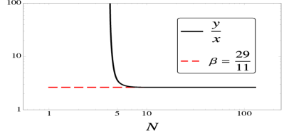
(a)

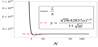
(b)

(c)

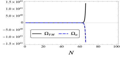
(d)

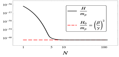
(e)

(f)

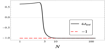
(g)

Figure 1: Dark energy - Numerical solutions and asymptotes for $\alpha=0.01$, $g=-4.37\times 10^{-61}$, and initial conditions $x_{0}=-0.187568$, $y_{0}=2$, and $z_{0}=7\times 10^{27}$. a) This figure shows the numerical solution for $y/x$ vs. $N$ (black continuous curve) as well as the asymptotic behaviour $y/x=\beta$ (red dashed curve) with $\beta$ as in Eq. (21); the pair of curves overlap from $N\approx 10$ onwards. b) Same as before but for $z/x$. c) This figure confirms that $\rho_{\alpha}\rightarrow-\rho_{\rm YM}$ in the asymptotic limit. d) This figure presents $\Omega_{\rm YM}$ vs. $N$ (black continuous curve) and $\Omega_{\alpha}$ vs. $N$ (blue dashed curve); we can see that the absolute values of the two density parameters grow exponentially with $N$. e) This figure presents $H/m_{P}$ vs. $N$; although $\rho_{\rm YM}$ and $|\rho_{\alpha}|$ grow exponentially, $\rho_{\rm tot}\propto\sqrt{H}$ approaches asymptotically a finite constant value. f) This figure shows $\omega_{\alpha}$ vs. $N$; in the asymptotic limit, the negative fluid behaves as radiation. g) This figure shows $\omega_{\rm tot}$ vs. $N$; in the asymptotic limit, the total fluid behaves as a cosmological constant.

Negative values for $\alpha$ would render $\gamma\in\mathbb{C}$ disabling the asymptotic behaviour; in contrast, positive and negative values for $g$ are allowed. Figs. 1a and 1b show the asymptotic behaviour for $y/x$ and $z/x$ for a chosen set of initial conditions. As stated before, the system exhibits an asymptotic dynamical fine-tuning mechanism, as the absolute values of the energy densities of the negative fluid ($|\rho_{\alpha}|$) and of the positive fluid ($\rho_{\rm YM}$) grow exponentially but, nevertheless, matches almost precisely, irrespective of the initial conditions, so that $\rho_{\rm tot}=\rho_{\rm YM}+\rho_{\alpha}$ approaches a finite constant value. To see this, we can easily extract $\Omega_{\alpha}\equiv\rho_{\alpha}/\rho_{\rm tot}$ and $\Omega_{\rm YM}\equiv\rho_{\rm YM}/\rho_{\rm tot}$ from Eq. (12):

$$\Omega_{\rm YM} = y^{2}+2xy+x^{2}+2g^{2}z^{4}\,,$$

$$\Omega_{\alpha} = \alpha(-32y^{4}-188xy^{3}+10x^{2}y^{2})\,,$$ (22)

and check that in the asymptotic limit given by Eqs. (20) and (21), $\rho_{\alpha}\rightarrow-\rho_{\rm YM}$. This is confirmed by the numerical solution presented in Fig. 1c. Fig. 1d shows the exponential growth with $N$ of both $\Omega_{\rm YM}$ and $|\Omega_{\alpha}|$ whereas Fig. 1e reveals the predicted behaviour for $\rho_{\rm tot}\propto\sqrt{H}$. As observed in the figures, the apparent breakdown of the classical regime due to the exponential growth of the absolute values of the energy densities is disproved by the good behaviour of $H<m_{P}$. The equation of state parameter for each fluid can also be studied by extracting the pressures $P_{\rm YM}$ and $P_{\alpha}$ from Eqs. (12) and (13):

$$P_{\rm YM} = \frac{\rho_{\rm tot}}{3}(y^{2}+2xy+x^{2}+2g^{2}z^{4})\,,$$

$$P_{\alpha} = \frac{\rho_{\rm tot}}{3}[\alpha(-340y^{4}+124y^{4}\epsilon+316xy^{3}$$ (23)

$$+614x^{2}y^{2}+104\sqrt{2}y^{3}p)]\,.$$

Of course, $\omega_{\rm YM}=1/3$, whereas $\omega_{\alpha}$ is a complicated function of $N$ that goes, in the asymptotic limit given by Eqs. (20) and (21), to $1/3$; this is numerically confirmed in Fig. 1f. Regarding the equation of state parameter for the whole fluid, we have asymptotically $\omega_{\rm tot}\rightarrow-1$; this is analytically the case as shown just below Eq. (21) and it is numerically confirmed in Fig. 1g. Such an interesting built-in self-tuning mechanism to generate an equation of state parameter $\omega\simeq-1$, in agreement with the observed equation of state parameter for dark energy $\omega=-1.006\pm 0.045$ Ade et al. (2016a, b), could not be an ideal candidate to explain the dark energy if the asymptotic value for $H$ did not correspond to the observed value today $H_{0}=9.03h\times 10^{-61}m_{P}$ with $h=0.678\pm 0.009$ Ade et al. (2016a). From the definitions in Eq. (11) and the asymptotic behaviour described in Eqs. (20) and (21), we obtain

$$\frac{H}{m_{P}}\rightarrow\left(\frac{\beta}{\gamma}\right)^{2}=\frac{29|g|}{\sqrt{42837\alpha}}\,,$$ (24)

which is consistent with the numerical solution for $H$ in Fig. 1e. This reveals that $H$ can reproduce its presently observed value for a low enough value of $|g|$: $|g|\lesssim 7H_{0}/m_{P}\approx 4\times 10^{-60}$, irrespective of the initial conditions (for $\alpha>0$, see footnote 6). The insensitivity to the initial conditions can be observed comparing Figs. 1 and 2.

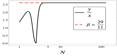
(a)

(b)

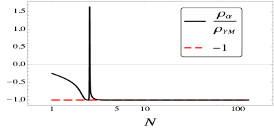
(c)

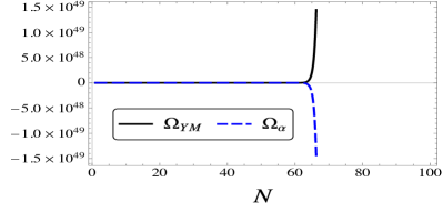
(d)

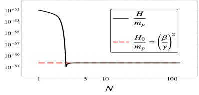
(e)

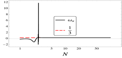
(f)

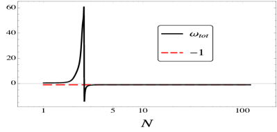
(g)

Figure 2: Dark energy - Same as Fig. 1 but with a different set of initial conditions: $x_{0}=0.998999$, $y_{0}=10^{-3}$, and $z_{0}=10^{22}$.

Primordial inflation - Aside the asymptotic behaviour, the critical points of the dynamical system in Eqs. (17) - (19) have also been studied. There exist 112 critical points, 51 of them being unrealistic as they correspond either to complex values for $y$ or $z$ or to real values for the same variables but with different signs, other 38 lead to $\epsilon\geq 1$, other 6 lead to $\epsilon<0$ and the other 17 lead to $0\leq\epsilon<1$. The latter ones are of special interest because they represent non-phantom accelerated expansion which, eventually, could be long enough but of finite duration to be ideal candidates to explain the primordial inflation. 8 out of these 17 critical points are unrealistic too because the inflationary period is only given for $H\rightarrow\infty$. From the remaining 9 critical points, 8 are uninteresting, most of them because inflation is very short (a few efolds). So we are left with 1 critical point, a saddle point indeed, that satisfies all the properties to be identified with a primordial inflationary period as described in Fig. 3. Unfortunately, and in contrast to the dark energy scenario, the primordial inflation in this model is strongly sensitive to the initial conditions and coupling constant $\alpha$.

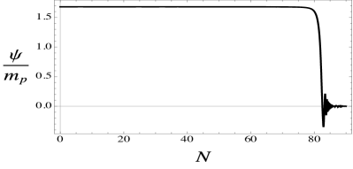
(a)

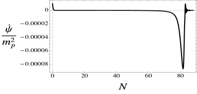
(b)

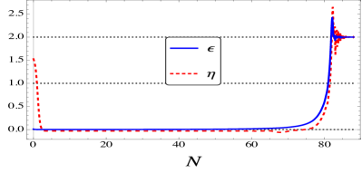
(c)

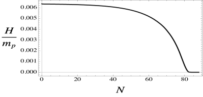
(d)

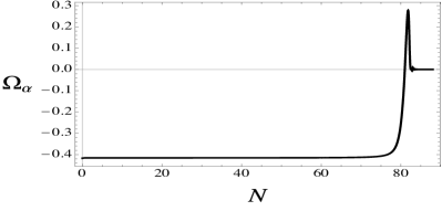
(e)

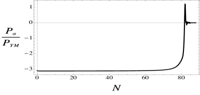
(f)

Figure 3: Primordial inflation - Numerical solutions for $\alpha=0.00649$, $g=-0.0001$, and initial conditions $x_{0}=0.0011$, $y_{0}=1.189$, and $z_{0}=14.911$. a) This figure exhibits the slow-roll behaviour of $\psi/m_{P}$ during some 70 efolds and a final stage of damped oscillations signalling the radiation dominated epoch. b) Similar behaviour as in the previous figure but for $\dot{\psi}/m_{P}^{2}$. c) This figure presents the slow-roll parameters $\epsilon$ (blue continuous curve) and $\eta$ (dashed red curve) vs. $N$; we can see that both $\epsilon$ and $|\eta|$ are well below 1 during some 70 efolds, implying a period of slow-roll inflation long enough to solve the classical problems of the standard cosmology; at the end of this stage, $\epsilon$ and $\eta$ go to 2, signalling the radiation dominated epoch. d) This figure presents $H/m_{P}$ vs. $N$; the energy scale of inflation is not in conflict with our classical treatment for low enough values of $|g|$. e) This figure shows $\Omega_{\alpha}$ vs. $N$; the $S$ term during inflation contributes with a negative energy density which is neither dominating nor negligible; it, nevertheless, becomes negligible by the end of this period. f) This figure shows $P_{\alpha}/P_{\rm YM}$ vs. $N$; the $S$ term during inflation contributes with a dominating negative pressure that becomes negligible by the end of this period letting the Yang-Mills term dominate and produce the radiation dominated epoch.

Further exploration of the model - The model presented above is so attractive, plausible, and well founded, at least as dark energy is concerned, that deserves further exploration. One of the first things to do is to investigate whether the Hamiltonian is actually bounded from below. In addition, a complete study of the cosmological perturbations is required in order to establish the robustness of the model against Laplacian and ghost instabilities, to check the perturbative stability of the isotropic solution, and to calculate the sound speed $c_{s}$ which is a distinctive feature of any dark energy model Hu and Eisenstein (1999). Another aspect to explore is the possible attractor nature of the triad configuration in a more general anisotropic background (as is done for the Gauge-flation model in Ref. Maleknejad et al. (2012)). However, what is an urgent and necessary matter to investigate is whether the addition of $\kappa\mathcal{L}_{4}^{2}$ can evade the apparently strong constraints coming from the detection of the gravitational wave signal GW170817 Abbott et al. (2017a) and its electromagnetic counterpart GRB 170817A Abbott et al. (2017b, c): a preliminary analysis, following the lines of Ref. Hertzberg and Sandora (2017), suggest that the coupling with the Riemann tensor in Eq. (3) does not modify the gravitational waves speed; this suggestion is strengthened by the fact that $\mathcal{L}_{6}$ in the generalized Proca theory for an Abelian vector field, which contains a coupling between two gauge field strength tensors and the double dual Riemann tensor, is not constrained as it does not alter the gravitational waves speed Baker et al. (2017) . The harmful terms seem then to be the couplings with the Ricci scalar. Thus, an adequate relation between the $\alpha$ and $\kappa$ parameters in $\alpha\mathcal{L}_{4}^{1}+\kappa\mathcal{L}_{4}^{2}\subset\mathcal{L}_{4}$ could deactivate the apparently harmful effect of the couplings with the Ricci scalar, at least for the cosmic triad configuration, making of this model a phenomenologically viable alternative. Of course, if this is possible, the cosmological implications of $\alpha\mathcal{L}_{4}^{1}+\kappa\mathcal{L}_{4}^{2}$ must be studied having in mind that the dark energy mechanism presented in this paper might not be counterbalanced by $\kappa\mathcal{L}_{4}^{2}$ . We expect to address this issue in a forthcoming publication.

Acknowledgements - This work was supported by the following grants: Colciencias - 123365843539 CT-FP44842-081-2014, DIEF de Ciencias - UIS - 2312, VCTI - UAN - 2017239, and Centro de Investigaciones - USTA - GIDPTOBASIC-UISUANUVALLEP12017. We want to acknowledge Alejandro Guarnizo, Luis Gabriel Gómez, Fabio Duván Lora, César Alonso Valenzuela, Carlos Mauricio Nieto, and Miguel Zumalacárregui for useful discussions and help at different stages of this project. Y. R. wants to give a special acknowledgement to Erwan Allys and Patrick Peter, who the generalized $SU(2)$ Proca theory was constructed with, for very instructive discussions, valuable help, and for sharing some research objectives.

References

- Weinberg (1996) S. Weinberg, The quantum theory of fields. Vol. 2: Modern applications (Cambridge University Press, 1996).
- Beltrán Jimenez and Heisenberg (2016) J. Beltrán Jimenez and L. Heisenberg, “Derivative self-interactions for a massive vector field,” Phys. Lett. B 757, 405–411 (2016), arXiv:1602.03410 [hep-th] .
- Allys et al. (2016a) E. Allys, J. P. Beltr n Almeida, P. Peter, and Y. Rodr guez, “On the 4D generalized Proca action for an Abelian vector field,” JCAP 1609, 026 (2016a), arXiv:1605.08355 [hep-th] .
- Rodr guez and Navarro (2017) Y. Rodr guez and A. A. Navarro, “Scalar and vector Galileons,” Proceedings, 70&70 Classical and Quantum Gravitation Party: Meeting with Two Latin American Masters on Theoretical Physics: Cartagena, Colombia, September 28-30, 2016, J. Phys. Conf. Ser. 831, 012004 (2017), arXiv:1703.01884 [hep-th] .
- Heisenberg (2017) L. Heisenberg, “Generalised Proca Theories,” in 52nd Rencontres de Moriond on Gravitation (Moriond Gravitation 2017) La Thuile, Italy, March 25-April 1, 2017 (2017) arXiv:1705.05387 [hep-th] .
- Maleknejad et al. (2013) A. Maleknejad, M. M. Sheikh-Jabbari, and J. Soda, “Gauge Fields and Inflation,” Phys. Rept. 528, 161–261 (2013), arXiv:1212.2921 [hep-th] .
- Soda (2012) J. Soda, “Statistical Anisotropy from Anisotropic Inflation,” Class. Quant. Grav. 29, 083001 (2012), arXiv:1201.6434 [hep-th] .
- Dimopoulos (2012) K. Dimopoulos, “Statistical Anisotropy and the Vector Curvaton Paradigm,” Int. J. Mod. Phys. D 21, 1250023 (2012), [Erratum: Int. J. Mod. Phys. D 21,1292003 (2012)], arXiv:1107.2779 [hep-ph] .
- Armendariz-Picon (2004) C. Armendariz-Picon, “Could dark energy be vector-like?” JCAP 0407, 007 (2004), arXiv:astro-ph/0405267 .
- Allys et al. (2016b) E. Allys, P. Peter, and Y. Rodr guez, “Generalized SU(2) Proca Theory,” Phys. Rev. D 94, 084041 (2016b), arXiv:1609.05870 [hep-th] .
- Baker et al. (2017) T. Baker, E. Bellini, P. G. Ferreira, M. Lagos, J. Noller, and I. Sawicki, “Strong constraints on cosmological gravity from GW170817 and GRB 170817A,” Phys. Rev. Lett. 119, 251301 (2017), arXiv:1710.06394 [astro-ph.CO] .
- Creminelli and Vernizzi (2017) P. Creminelli and F. Vernizzi, “Dark Energy after GW170817 and GRB170817A,” Phys. Rev. Lett. 119, 251302 (2017), arXiv:1710.05877 [astro-ph.CO] .
- Sakstein and Jain (2017) J. Sakstein and B. Jain, “Implications of the Neutron Star Merger GW170817 for Cosmological Scalar-Tensor Theories,” Phys. Rev. Lett. 119, 251303 (2017), arXiv:1710.05893 [astro-ph.CO] .
- Ezquiaga and Zumalac rregui (2017) J. M. Ezquiaga and M. Zumalac rregui, “Dark Energy After GW170817: Dead Ends and the Road Ahead,” Phys. Rev. Lett. 119, 251304 (2017), arXiv:1710.05901 [astro-ph.CO] .
- Wang et al. (2017) H. Wang et al., “The GW170817/GRB 170817A/AT 2017gfo Association: Some Implications for Physics and Astrophysics,” Astrophys. J. 851, L18 (2017), arXiv:1710.05805 [astro-ph.HE] .
- Abbott et al. (2017a) B. P. Abbott et al. (Virgo, LIGO Scientific), “GW170817: Observation of Gravitational Waves from a Binary Neutron Star Inspiral,” Phys. Rev. Lett. 119, 161101 (2017a), arXiv:1710.05832 [gr-qc] .
- Abbott et al. (2017b) B. P. Abbott et al. (GROND, SALT Group, OzGrav, DFN, INTEGRAL, Virgo, Insight-Hxmt, MAXI Team, Fermi-LAT, J-GEM, RATIR, IceCube, CAASTRO, LWA, ePESSTO, GRAWITA, RIMAS, SKA South Africa/MeerKAT, H.E.S.S., 1M2H Team, IKI-GW Follow-up, Fermi GBM, Pi of Sky, DWF (Deeper Wider Faster Program), Dark Energy Survey, MASTER, AstroSat Cadmium Zinc Telluride Imager Team, Swift, Pierre Auger, ASKAP, VINROUGE, JAGWAR, Chandra Team at McGill University, TTU-NRAO, GROWTH, AGILE Team, MWA, ATCA, AST3, TOROS, Pan-STARRS, NuSTAR, ATLAS Telescopes, BOOTES, CaltechNRAO, LIGO Scientific, High Time Resolution Universe Survey, Nordic Optical Telescope, Las Cumbres Observatory Group, TZAC Consortium, LOFAR, IPN, DLT40, Texas Tech University, HAWC, ANTARES, KU, Dark Energy Camera GW-EM, CALET, Euro VLBI Team, ALMA), “Multi-messenger Observations of a Binary Neutron Star Merger,” Astrophys. J. 848, L12 (2017b), arXiv:1710.05833 [astro-ph.HE] .
- Abbott et al. (2017c) B. P. Abbott et al. (Virgo, Fermi-GBM, INTEGRAL, LIGO Scientific), “Gravitational Waves and Gamma-rays from a Binary Neutron Star Merger: GW170817 and GRB 170817A,” Astrophys. J. 848, L13 (2017c), arXiv:1710.05834 [astro-ph.HE] .
- Deffayet and Steer (2013) C. Deffayet and D. A. Steer, “A formal introduction to Horndeski and Galileon theories and their generalizations,” Class. Quant. Grav. 30, 214006 (2013), arXiv:1307.2450 [hep-th] .
- Ostrogradski (1850) M. Ostrogradski, “Memoires sur les equations differentielles relatives au probleme des isoperimetres,” Mem. Ac. St. Petersbourg VI, 385 (1850).
- Woodard (2007) R. P. Woodard, “Avoiding dark energy with 1/r modifications of gravity,” The invisible universe: Dark matter and dark energy. Proceedings, 3rd Aegean School, Karfas, Greece, September 26-October 1, 2005, Lect. Notes Phys. 720, 403–433 (2007), arXiv:astro-ph/0601672 .
- Woodard (2015) R. P. Woodard, “Ostrogradsky’s theorem on Hamiltonian instability,” Scholarpedia 10, 32243 (2015), arXiv:1506.02210 [hep-th] .
- Horndeski (1974) G. W. Horndeski, “Second-order scalar-tensor field equations in a four-dimensional space,” Int. J. Theor. Phys. 10, 363–384 (1974).
- Nicolis et al. (2009) A. Nicolis, R. Rattazzi, and E. Trincherini, “The Galileon as a local modification of gravity,” Phys. Rev. D 79, 064036 (2009), arXiv:0811.2197 [hep-th] .
- Deffayet et al. (2009a) C. Deffayet, G. Esposito-Farese, and A. Vikman, “Covariant Galileon,” Phys. Rev. D 79, 084003 (2009a), arXiv:0901.1314 [hep-th] .
- Deffayet et al. (2009b) C. Deffayet, S. Deser, and G. Esposito-Farese, “Generalized Galileons: All scalar models whose curved background extensions maintain second-order field equations and stress-tensors,” Phys. Rev. D 80, 064015 (2009b), arXiv:0906.1967 [gr-qc] .
- Deffayet et al. (2011) C. Deffayet, X. Gao, D. A. Steer, and G. Zahariade, “From k-essence to generalised Galileons,” Phys. Rev. D 84, 064039 (2011), arXiv:1103.3260 [hep-th] .
- Kobayashi et al. (2011) T. Kobayashi, M. Yamaguchi, and J. Yokoyama, “Generalized G-inflation: Inflation with the most general second-order field equations,” Prog. Theor. Phys. 126, 511–529 (2011), arXiv:1105.5723 [hep-th] .
- Horndeski (1976) G. W. Horndeski, “Conservation of Charge and the Einstein-Maxwell Field Equations,” J. Math. Phys. 17, 1980–1987 (1976).
- Deffayet et al. (2014) C. Deffayet, A. E. G mr k oglu, S. Mukohyama, and Y. Wang, “A no-go theorem for generalized vector Galileons on flat spacetime,” JHEP 1404, 082 (2014), arXiv:1312.6690 [hep-th] .
- Heisenberg (2014) L. Heisenberg, “Generalization of the Proca Action,” JCAP 1405, 015 (2014), arXiv:1402.7026 [hep-th] .
- Tasinato (2014a) G. Tasinato, “Cosmic Acceleration from Abelian Symmetry Breaking,” JHEP 1404, 067 (2014a), arXiv:1402.6450 [hep-th] .
- Hull et al. (2016) M. Hull, K. Koyama, and G. Tasinato, “Covariantized vector Galileons,” Phys. Rev. D 93, 064012 (2016), arXiv:1510.07029 [hep-th] .
- Allys et al. (2016c) E. Allys, P. Peter, and Y. Rodríguez, “Generalized Proca action for an Abelian vector field,” JCAP 1602, 004 (2016c), arXiv:1511.03101 [hep-th] .
- Beltran Jimenez and Heisenberg (2017) J. Beltran Jimenez and L. Heisenberg, “Generalized multi-Proca fields,” Phys. Lett. B 770, 16–26 (2017), arXiv:1610.08960 [hep-th] .
- Maleknejad and Sheikh-Jabbari (2013) A. Maleknejad and M. M. Sheikh-Jabbari, “Gauge-flation: Inflation From Non-Abelian Gauge Fields,” Phys. Lett. B 723, 224–228 (2013), arXiv:1102.1513 [hep-ph] .
- Maleknejad and Sheikh-Jabbari (2011) A. Maleknejad and M. M. Sheikh-Jabbari, “Non-Abelian Gauge Field Inflation,” Phys. Rev. D 84, 043515 (2011), arXiv:1102.1932 [hep-ph] .
- Adshead and Wyman (2012) P. Adshead and M. Wyman, “Chromo-Natural Inflation: Natural inflation on a steep potential with classical non-Abelian gauge fields,” Phys. Rev. Lett. 108, 261302 (2012), arXiv:1202.2366 [hep-th] .
- Nieto and Rodr guez (2016) C. M. Nieto and Y. Rodr guez, “Massive Gauge-flation,” Mod. Phys. Lett. A 31, 1640005 (2016), arXiv:1602.07197 [gr-qc] .
- Adshead et al. (2016) P. Adshead, E. Martinec, E. I. Sfakianakis, and M. Wyman, “Higgsed Chromo-Natural Inflation,” JHEP 1612, 137 (2016), arXiv:1609.04025 [hep-th] .
- Adshead and Sfakianakis (2017) P. Adshead and E. I. Sfakianakis, “Higgsed Gauge-flation,” JHEP 1708, 130 (2017), arXiv:1705.03024 [hep-th] .
- Davydov and Galtsov (2016) E. Davydov and D. Galtsov, “HYM-flation: Yang-Mills cosmology with Horndeski coupling,” Phys. Lett. B 753, 622–628 (2016), arXiv:1512.02164 [hep-th] .
- Maleknejad et al. (2012) A. Maleknejad, M. M. Sheikh-Jabbari, and J. Soda, “Gauge-flation and Cosmic No-Hair Conjecture,” JCAP 1201, 016 (2012), arXiv:1109.5573 [hep-th] .
- de Felice et al. (2017) A. de Felice, L. Heisenberg, and S. Tsujikawa, “Observational constraints on generalized Proca theories,” Phys. Rev. D 95, 123540 (2017), arXiv:1703.09573 [astro-ph.CO] .
- De Felice et al. (2016a) A. De Felice, L. Heisenberg, R. Kase, S. Mukohyama, S. Tsujikawa, and Y.-l. Zhang, “Effective gravitational couplings for cosmological perturbations in generalized Proca theories,” Phys. Rev. D 94, 044024 (2016a), arXiv:1605.05066 [gr-qc] .
- De Felice et al. (2016b) A. De Felice, L. Heisenberg, R. Kase, S. Mukohyama, S. Tsujikawa, and Y.-l. Zhang, “Cosmology in generalized Proca theories,” JCAP 1606, 048 (2016b), arXiv:1603.05806 [gr-qc] .
- Tasinato (2014b) G. Tasinato, “A small cosmological constant from Abelian symmetry breaking,” Class. Quant. Grav. 31, 225004 (2014b), arXiv:1404.4883 [hep-th] .
- Emami et al. (2017) R. Emami, S. Mukohyama, R. Namba, and Y.-l. Zhang, “Stable solutions of inflation driven by vector fields,” JCAP 1703, 058 (2017), arXiv:1612.09581 [hep-th] .
- Ade et al. (2016a) P. A. R. Ade et al. (Planck), “Planck 2015 results. XIII. Cosmological parameters,” Astron. Astrophys. 594, A13 (2016a), arXiv:1502.01589 [astro-ph.CO] .
- Ade et al. (2016b) P. A. R. Ade et al. (Planck), “Planck 2015 results. XIV. Dark energy and modified gravity,” Astron. Astrophys. 594, A14 (2016b), arXiv:1502.01590 [astro-ph.CO] .
- Hu and Eisenstein (1999) W. Hu and D. J. Eisenstein, “The Structure of structure formation theories,” Phys. Rev. D 59, 083509 (1999), arXiv:astro-ph/9809368 .
- Hertzberg and Sandora (2017) M. P. Hertzberg and M. Sandora, “General Relativity from Causality,” JHEP 1709, 119 (2017), arXiv:1702.07720 [hep-th] .
- Bettoni et al. (2017) D. Bettoni, J. M. Ezquiaga, K. Hinterbichler, and M. Zumalac rregui, “Speed of Gravitational Waves and the Fate of Scalar-Tensor Gravity,” Phys. Rev. D 95, 084029 (2017), arXiv:1608.01982 [gr-qc] .
- Lombriser and Taylor (2016) L. Lombriser and A. Taylor, “Breaking a Dark Degeneracy with Gravitational Waves,” JCAP 1603, 031 (2016), arXiv:1509.08458 [astro-ph.CO] .
- Brax et al. (2016) P. Brax, C. Burrage, and A.-C. Davis, “The Speed of Galileon Gravity,” JCAP 1603, 004 (2016), arXiv:1510.03701 [gr-qc] .
- Arai and Nishizawa (2017) S. Arai and A. Nishizawa, “Generalized framework for testing gravity with gravitational-wave propagation. II. Constraints on Horndeski theory,” (2017), arXiv:1711.03776 [gr-qc] .