Non-equilibrium evolution of quantum fields during inflation and late accelerating expansion

Abstract

To understand mechanisms leading to inflation and late acceleration of the Universe it is important to see how one or a set of quantum fields may evolve such that the classical energy-momentum tensor behave similar to a cosmological constant. Phenomenological models assume that condensation of a scalar field dominating other constituents is responsible for the onset of inflation and dark energy. However, conditions for formation of such a condensate and whether it is a necessary ingredient for generation of inflation and late acceleration are not clear. In this work we consider a toy model including 3 scalar fields with very different masses to study the formation of a light axion-like condensate, presumed to be responsible for inflation and/or late accelerating expansion of the Universe. Despite its simplicity, this model reflects hierarchy of masses and couplings of the Standard Model and its candidate extensions. The investigation is performed in the framework of non-equilibrium quantum field theory in a consistently evolved FLRW geometry. We discuss in details how the initial conditions for such a model must be defined in a fully quantum setup and show that in a multi-component model interactions reduce the number of independent initial degrees of freedom. Numerical simulation of this model shows that it can be fully consistent with present cosmological observations. For the chosen range of parameters we find that quantum interactions rather than effective potential of a condensate is the dominant contributor in the energy density of the Universe and triggers both inflation and late accelerating expansion. Nonetheless, despite its small contribution in the energy density, the light scalar field - in both condensate and quasi free particle forms - has a crucial role in controlling the trend of heavier fields. Furthermore, up to precision of our simulations we do not find any IR singularity during inflation. These findings highlight uncertainties in attempts to extract information about physics of the early Universe by naively comparing predictions of local effective classical models with cosmological observations, neglecting inherently non-local nature of quantum processes.

1 Introduction

Cosmological observations have demonstrated that at least during two epochs the Universe has gone through accelerating expansion. The first era, usually called inflation [1] occurred at or close to the birth of the Universe. The second epoch has begun at around redshift 0.5 - roughly half of the age of the Universe - and is ongoing now. Its unknown cause is given the generic name of dark energy [2, 3] (reviews) and at present it is the dominant contributor in the average energy density of the Universe. If dark energy is not an elusive Cosmological Constant (CC), its origin may be a modification of Einstein theory of gravity or a new field in the matter side of the Einstein equation [4]. It is possible that inflation and dark energy be the manifestation of the same phenomenon at different epochs [6] (review). Homogeneity of present expansion rate [7] and properties of inflation concluded from observations of the Cosmic Microwave Background (CMB) anisotropies [8] indicate a slowly varying - in both space and time - energy density for dark energy and inflaton. This requirement can be phenomenologically formulated with one or multiple light quantum scalar fields, which their effective flat potential dominates the energy density of the Universe during the epochs of accelerating expansion.

In two ways a quantum field may generate an effective flat energy-momentum tensor: either through non-zero 1-point Green’s function - also called condensate, mean, or background field - of a scalar (or vector) field $\varphi\equiv\langle\Phi\rangle\neq 0$ and its close to flat potential; or through quantum interactions producing an approximately constant average energy density and small quantum fluctuations around it. Even in the latter case, which corresponds to a subdominant contribution of condensate in the energy density of the Universe and in the expansion rate, the condensate may have a crucial role in cosmological phenomena through Higgs mechanism and breaking of symmetries [9] (reviews). Thus, motivations for investigating formation and evolution of condensates in cosmology go beyond their role in inflation and late accelerating expansion.

Evolution of quantum scalar fields in curved spacetimes are extensively studied, specially in de Sitter geometry as a good approximation for the geometry of the Universe during inflation and reheating [10]. For instance, authors of [11] study reheating and evolution of mean field (condensate) and their backreaction on the metric for an $O(N)$ symmetric multi-scalar field model. However, their formulation and simulations include only local quantum corrections to effective mass. In [12] the evolution of a pre-existing condensate during preheating for the same model as previous and thermalization of quantum fluctuations are studied. Their simulations consistently evolve geometry and take into account non-local quantum corrections to effective potential. But, they are performed for unrealistically large couplings. Models with more diverse field content are also studied [13, 14], mostly in de Sitter space and without backreaction on the geometry. The common aim of practically all these and many other works in the literature have been the study of particle production during and after inflation. Estimation of non-Gaussianity generated by quantum processes is another topic related to inflation which is extensively investigated [15]. However, by the nature of this subject, the concentration has been on the quantum correlation of fluctuations rather than effective secular component driving inflation itself. In fact, the onset and evolution of quantum field(s) leading to a shallow slope effective potential for the condensate or all components and onset of an inflationary era from a pre-inflationary epoch is not extensively studied.

A controversial issue about inflation, which is not yet completely settled, is the stability of IR modes. Instability of these modes, and thereby the de Sitter geometry, is first concluded in [16]. Its effect on the evolution of inflation and de Sitter geometry is studied in [17]. The particular case of massless scalar fields is investigated in [18, 19] (using parametric representation of path integrals, and adiabatic vacuum subtraction renormalization, respectively). Breaking of symmetries by condensation of light scalars, acquisition of mass by some fields, and generation of massless Goldstone modes for others are investigated in [20] (using Winger-Weisskopf method [21]). In addition, analogy between particle creation and vacuum instability in a constant electric field and de Sitter space vacuum is used to study the IR instability of the latter models in [16]. It is also shown that subhorizon and superhorizon modes become entangled when a transition from fast roll to slow roll occurs. This convoys the effect of non-observable IR singularities to observable subhorizon fluctuations. Furthermore, sudden variations of inflaton field(s) lead to particle production, suppression of dynamical mass, and anomalous decay of inflaton [23]. Quantum IR modes and ultra light particles are also suggested as the origin of dark energy [24].

Furthermore, a fully non-equilibrium quantum field theoretical calculation of IR modes in de Sitter space [26] shows that due to dynamical acquisition of mass by a massless scalar, these modes are naturally regulated and no singularity arises. Other works using the same method [27] confirm these results for inflaton alone, but find that IR quantum corrections become large and non-perturbative in curvaton models, which include spectator scalar field(s). Other perturbative and non-perturbative methods are also used to investigate the issue of IR modes. For instance, in [22] parametric representation of path integrals are used to show that de Sitter space is instability-free in presence of massive fields, in contrast to the case of massless fields studied with the same method by the same authors. Non-perturbative renormalization group technique is used by [28] to find quantum corrections to classical potential of $O(N)$ model in de Sitter space. They conclude that due to large IR fluctuations symmetries are radiatively restored, i.e. no condensate is formed. However, their calculation includes only local quantum corrections and solutions of free field equation are used to estimate the evolution of condensate. These approximations do not seem reasonable when the issue of large distant correlations is studied. Stochastic approach to inflation [29, 30] is used by [31] to take into account, in a non-perturbative manner, quantum corrections to the same model as previous works cited here. The equivalence of stochastic and Schwinger-Keldysh 2 Particle Irreducible (2PI) method for IR modes is shown in [32]. They conclude that no condensate is formed and symmetry of the $O(N)$ model is preserved.

In what concerns the estimation of long distance correlations and formation of a condensate, which may lead to symmetry breaking, one of the main shortcoming of works reviewed above is neglecting the backreaction of quantum effects on the evolution of geometry. This issue is an addition to other approximations which had to be considered to make models analytically tractable. Moreover, these studies have been mostly concentrated on a single field or $O(N)$ symmetry inflaton, and exceptionally on models with additional fields possessing mass and coupling hierarchies. Additionally, the issue of condensate formation and symmetry breaking needs more accurate calculation than what have been done in previous works, because analytical approximations may have important and misleading impact on conclusions - we will discuss an example of such problems later in this work. Although formal description of perturbative expansion and Feynman diagrams contributing in the evolution of condensates are worked out in details in [33], an analytical approach including consistent evolution of geometry is not available.

Studies of dark energy models in full quantum field theoretical setups are very rare. Example of exceptions are [24, 34, 35, 5]. However, even these works miss some of the most important features which a simple but realistic model should cover, namely: taking into account both local and nonlocal quantum corrections, at least at lowest order; backreaction of matter on the geometry; mass hierarchy; proper calculation of formation and evolution of condensate, etc. Indeed many dark energy models are simply phenomenological and do not have a well defined and renormalizable quantum formulation. In particular, in many modified gravity models - as an alternative to a cosmological constant - the dilaton scalar field has a non-standard and non-renormalizable Lagrangian. These models must be considered as effective theories and their quantization is either meaningless or must be restricted to lowest order to avoid renormalization issues. By contrast, the class of models generally called interacting quintessence include cases with quantum mechanically well defined and renormalizable interactions, such as a monomial/polynomial $\phi^{n}$-type self-interaction [36] with $n>0$ or a gauge field [37]. We should remind that despite various definitions and classification procedures in the literature [38, 39, 40], there is not a general consensus about how a dark energy model should be classified as modified gravity or quintessence. Here we use the definition of [39]: if the scalar field responsible for accelerating expansion has the same coupling to all fields, including itself, the model is considered to be a modified gravity; otherwise it is called (interacting)-quintessence.

As we mentioned above little work has been performed on the formation of a condensate. Specifically, studies of inflation, reheating, and dark energy models usually assume a pre-existing condensate as initial condition. Therefore, our aim is to understand how a condensate is formed from an initial state where it is absent. Another goal is to understand whether and under which conditions it may become energetically dominant, as it is usually assumed in classical approaches to inflation and dark energy. For this purpose, in a previous work [35] we studied formation and evolution of the condensate of a light scalar produced by the decay of a massive particle in FLRW geometry. The model includes 3 fields which present the three important mass scales, namely a heavy field presenting sub-Planckian/GUT physics, an axion-like light field as inflaton or quintessence field, and an intermediate mass field presenting Standard Model particles. The calculation takes into account the lowest order quantum corrections to effective potential of condensate, but not quantum corrections to propagators. Nonetheless, this model stands out from those reviewed above by including fields with very different masses and in this respect it is a better representation of what we see in particle physics. This study showed that during radiation domination the amplitude of the condensate builds up very quickly - indeed similar to parametric resonance and particle production during preheating. But in matter domination era all but the longest modes decay. Moreover, only for self-interaction potentials of order $\lesssim 4$ long (IR) modes survive the faster expansion of the Universe. This result is consistent with conclusions of [13] about the evolution of inflation condensate. Furthermore, it is shown that only by taking into account quantum corrections the condensate may survive. Therefore, if dark energy is not due to an alternative gravity model, it may be a large scale non-local quantum phenomenon, which could not exist in the realm of a classical expanding universe. However, approximate analytical approach used in [35] works for a fixed geometry and backreaction of matter evolution on the geometry cannot be followed.

The goal of present work is to improve the investigation performed in [35] by using full 2PI formalism in a consistently evolved FLRW geometry according to a semi-classical Einstein equation. The toy model of [35] can be considered as an inflation model, interacting quintessence or both, because only initial conditions discriminate between these epochs. To go further than [35], it is important to properly evolve different components, specially the condensate, and investigate their role in the process of accelerating expansion and formation of anisotropies. Unfortunately, these goals cannot be accomplished analytically. Numerical simulations are necessary, and they have their own difficulties and imprecisions. Nonetheless, similar to other hard problems in theoretical physics, such as strong coupling regime of QCD and evolution of Large Scale Structures (LSS) of the Universe, the hope is that the quality of such simulations would be gradually improved.

In Sec. 2 we present the model. To fix notations a brief review of 2PI formulation is given in Sec. 2.1 and applied to the model in Sec. 2.2. Renormalization is discussed in Sec. 2.3. The semi-classical energy-momentum tensor and Einstein equation are obtained in Sec. 2.4. As the model includes 3 fields with very different masses, and apriori it can have a non-zero initial condensate, the initial state and initial conditions for solving dynamical equations must be chosen in a consistent way. These topics are discussed in Sec. 3. The issue of consistently defining and taking into account the contribution of non-vacuum initial state in the 2PI is not trivial [41, 42]. In the literature the case of a thermal initial condition is extensively studied [42]. But, in inflation and dark energy physics an initial coherent condensate state alone or along with a non-condensate is physically plausible and an interesting case to consider. In subsection 3.1 we discuss interesting initial states for the model. In particular, we determine the density matrix of a generalized coherent state and discuss its contribution in the generating functional of 2PI formalism. In Sec. 3.2 initial conditions for evolution equations of propagators and condensate are discussed. Initial conditions for the semi-classical Einstein equation is described in Sec. 3.3. We will show that they also fix the normalization of the wave-functions of constituents. Numerical simulations of the model and their results are presented in Sec. 4. Physical implications of the results of simulations are discussed in Sec. 5. Sec. 6 summarizes the outlines of this work.

In Appendix A we calculate extrema of classical potential of the model. Appendix B reminds the definition of various propagators and Appendix D presents description of free propagators with respect to solutions of evolution equations for a given initial state. In Appendix C we present the general description of initial state and density matrix. In Appendix E we obtain momentum distribution of remnants of a decaying heavy particle. Appendix F presents Christoffel coefficients for the linearized metric gauge used here. Appendix G reviews solutions of free evolution equation for cases of radiation and matter dominated homogeneous FLRW metric, and WKB approximation for other geometries and for renormalization of the model. Initial conditions described in Sec. 3 give a unique solution for integration constants of renormalized initial propagators and condensate. They are determined in Appendix H.

2 Model

We consider a phenomenological model with 3 scalar fields which their masses are in 3 physically interesting and relevant ranges: a heavy particle $X$ with a mass a few orders of magnitude less than Planck scale - presumably in GUT scale; a scalar field $A$ with an intermediate mass of order the of electroweak mass scale, that is in GeV-TeV range; and finally a vary light axion-like scalar $\Phi$. The model can be easily extended to the case in which $X$ and $A$ are fermions. Extension to vector fields and a full Yang-Mills model is also straightforward, but because of their additional complexities, we do not consider them here. We believe that the simplest case of scalars without internal symmetries is generic enough for investigating properties of condensate and effective potential, which may affect expansion of the Universe. In particular, the extension of the model to the case where each scalar field has an internal $O(N)$ symmetry only modifies multiplicity of Feynman diagrams. Such extensions are widely used in the literature in the framework of large $N$ expansion technique to take into account non-perturbative effects, see e.g. [44] for a recent review and [45] for its application in study of non-Gaussianity in cosmological models.

A similar model has been studied as an alternative to simple quintessence models for dark energy, classically in [46, 36] and with lowest quantum corrections in [35], and its extension to inflationary epoch may provide a unified theory for both phenomena. In addition, interaction between massive and light fields is known to influence the evolution of fluctuations [13], and thereby IR modes [14, 47] of both the condensate and quantum fluctuations. The third field with intermediate mass may be considered as a prototype of an average mass dark matter or Standard Model fields, if the heavy field is considered as a meta-stable dark matter.

Considering the simplest interactions between the 3 constituents of the model, the classical Lagrangian can be written as the following:

$${\mathcal{L}} = {\mathcal{L}}_{\Phi}+{\mathcal{L}}_{X}+{\mathcal{L}}_{A}+{\mathcal{L}}_{int}$$ (2.1)

$${\mathcal{L}}_{\Phi} = \int d^{4}x\sqrt{-g}\biggl{[}\frac{1}{2}g^{\mu\nu}{\partial}_{\mu}\Phi{\partial}_{\mu}\Phi-\frac{1}{2}m_{\Phi}^{2}{\Phi}^{2}-\frac{\lambda}{n!}{\Phi}^{n}\biggr{]}$$ (2.2)

$${\mathcal{L}}_{X} = \int d^{4}x\sqrt{-g}\biggl{[}\frac{1}{2}g^{\mu\nu}{\partial}_{\mu}X{\partial}_{\mu}X-\frac{1}{2}m_{X}^{2}X^{2}\biggr{]}$$ (2.3)

$${\mathcal{L}}_{A} = \int d^{4}x\sqrt{-g}\biggl{[}\frac{1}{2}g^{\mu\nu}{\partial}_{\mu}A{\partial}_{\mu}A-\frac{1}{2}m_{A}^{2}A^{2}-\frac{\lambda^{\prime}}{n^{\prime}!}A^{n^{\prime}}\biggr{]}$$ (2.4)

$${\mathcal{L}}_{int} = \int d^{4}x\sqrt{-g}\begin{cases}\mathsf{g}\Phi XA,&\quad\quad\text{(a)}\\ \mathsf{g}\Phi XA^{2},&\quad\quad\text{(b)}\\ \mathsf{g}{\Phi}^{2}XA,&\quad\quad\text{(c)}\end{cases}$$ (2.5)

Model (a) is the simplest interaction and in presence of an internal symmetry either $X$ is in the same representation as one of the other fields and the third one is a singlet, or it is singlet and $A$ and $\Phi$ are in conjugate representations. Other cases in (2.5) can have more diverse symmetry properties. In this work we only consider the model (a). Moreover, we assume that only $\Phi$ has a self interaction, thus $\lambda^{\prime}=0$. It is well known that quantum corrections increases the dynamical mass of $\Phi$. For this reason, usually a shift symmetry i.e. a periodic potential is assumed for light scalar fields [48]. But such potentials are not renormalizable perturbatively. Moreover, the assumption of small self-coupling and coupling to other fields ensures the suppression of high order corrections very quickly. Indeed numerical simulations discussed in Sec. 4.2.4 show that at the onset of inflation the effective mass of the scalar falls off at approaches its initial value. Although we are only interested in fully quantum treatment of the model, it is useful to know the classical behaviour of the system presented by Lagrangian (2.1), in particular extrema of its classical potential. They are calculated in Appendix A.

In [35] we found that the amplitude of the condensate decreases very rapidly with the mass of $\Phi$. This observation can understood as the following: Assume that condensates are coherent states as defined in Sec. 3.1.1. Because these states are quantum superposition of many particle states, heavier the field smaller is the probability of the production of a large number of particles. Therefore, it is expected that condensate component of $X$ and $A$ be subdominant. For this reason we ignore them to simplify the model and its numerical simulation.

2.1 2PI formalism

The method of effective action [49] - also called 2 Particle Irreducible (2PI) formalism - is closely related to Schwinger-Keldysh [50] and Kadanoff-Baym [51] equations, which generalize Boltzmann equation - more exactly BBGKY hierarchy - to describe non-equilibrium systems in the framework of quantum field theory. The advantage of 2PI is in the fact that all 1PI corrections are included in the propagators, and owing to integration over higher order corrections, better precision for amplitudes of processes can be achieved at a lower order of perturbative expansion, see for instance [44] for a recent review and example of applications. The 2PI formalism is also extended to curved spacetimes [52, 53].

The effective action depends on both 1-point $\varphi\equiv\langle\hat{\Phi}(x)\rangle$ and 2-point expectation values:

$$G(x,y)\equiv\langle\Psi|T\hat{\Phi}(x)\hat{\Phi}(y)|\Psi\rangle-\varphi(x)\varphi(y)=\langle\Psi|T\hat{\phi}(x)\hat{\phi}(y)|\Psi\rangle=\text{tr}(\hat{\rho}\hat{\phi}(x)\hat{\phi}(y))$$ (2.6)

$$\hat{\phi}\equiv\hat{\Phi}-I\varphi,\quad\quad\hat{\rho}\equiv|\Psi\rangle\langle\Psi|$$ (2.7)

where in Heisenberg picture the density matrix $\hat{\rho}$ is independent of time. Note that in the definition (2.6) we have omitted internal indices of fields. Indeed 2-point Green’s functions can be defined for two fields with different indices if the model has e.g. an $O(N)$ symmetry. We call these 2-point expectation values mixed propagators.

Using the definition of perturbatively free states in Appendix C, it is evident that a state with $\varphi\neq 0$ cannot contain finite number of particles. We call such a state a condensate. A general state $\rho$ can be a superposition of condensates and perturbatively free particles. The condensate component has its own fluctuations, which manifest themselves in time and position dependence of the classical field $\varphi$.

The density operator $\hat{\rho}$ can be a vacuum state or otherwise. In Minkowski spacetime vacuum state is defined as the state annihilated by number operator $\hat{N}_{\alpha}\equiv a_{\alpha}^{\dagger}a_{\alpha}$ for any mode $\alpha$. However, in curved spacetimes this definition is frame dependent, and under a general coordinate transformation such a state becomes a state with infinite number of particles [54]. An alternative definition of vacuum is a superposition of condensate states such that the amplitude of all components approaches zero [55]. It is shown that this vacuum state is annihilated by number operator in any frame. Through this work vacuum refers to such a state.

In 2PI formalism the effective action can be decomposed as [49, 52, 44]:

$$\Gamma[\{\varphi_{\alpha}\},\{G_{\alpha\beta}\}]=S[\{\varphi_{\alpha}\}]+\frac{i}{2}\biggl{(}tr[\ln G_{\alpha\beta}^{-1}]+tr[\mathcal{G}_{\alpha\beta}^{-1}G_{\alpha\beta}]\biggr{)}+\Gamma_{2}[\{\varphi_{\alpha}\},\{G_{\alpha\beta}\}]+const$$ (2.8)

From left to right the terms in the r.h.s. of (2.8) are classical action for condensates of quantum fields $\{\Phi_{\alpha}\}$, 1PI contribution, and 2PI contribution to the effective action $\Gamma[\{\varphi_{\alpha}\},\{G_{\alpha\beta}\}]$. Propagators $G_{\alpha\beta}$ are the 2-point Green’s functions defined in (2.6) for quantum fields $\hat{\Phi}_{\alpha}$ and $\hat{\Phi}_{\beta}$. The trace is taken over both flavor indices $\alpha$ and spacetime. The free propagator $\mathcal{G}_{\alpha\beta}$ is the second functional derivative of the classical action:

$$\mathcal{G}_{\alpha\beta}^{-1}(x,y)=i\delta_{\alpha\beta}\biggl{(}\frac{1}{\sqrt{-g}}{\partial}_{\mu}(\sqrt{-g}g^{\mu\nu}{\partial}_{\nu})+V^{\prime\prime}(\varphi_{\alpha})\biggr{)}\delta^{4}(x,y)$$ (2.9)

$$\int d^{4}x\sqrt{-g}~{}\delta^{4}(x,y)f(x)\equiv f(y),\quad\forall f$$ (2.10)

where $V$ is the interaction potential in the Lagrangian of the model. The propagator $G_{\alpha\beta}$ is assumed to contain all orders of perturbative quantum corrections and in this sens it is exact.

To fix notations and 2PI equations that we will apply to the model studied here, we briefly review how (2.8) is obtained. In the framework of Schwinger-Keldysh Closed Time Path integral (CTP) [50, 51] (also called in-in formalism) the generating functional $\mathcal{Z}[\varphi,G]$ of Feynman diagrams can be expanded as :

$$\mathcal{Z}(J_{a},K_{ab};\varrho) \equiv e^{iW[J_{a},K_{ab}]}=\int\mathcal{D}\Phi^{a}\mathcal{D}\Phi^{b}\exp\biggl{[}iS(\Phi^{a})+i\int d^{4}x\sqrt{-g}J_{a}(x)\Phi^{a}(x)+$$ (2.11)

$$\frac{i}{2}\int d^{4}xd^{4}y\sqrt{-g(x)}\sqrt{-g(y)}\Phi^{a}(x)K_{ab}(x,y)\Phi^{b}(y)\biggr{]}\langle\Phi^{a}|\hat{\varrho}|\Phi^{b}\rangle$$

where indices $a,b\in\{+,-\}$ indicate two opposite time branches. They are contracted by the diagonal tensor $c_{ab}\equiv\text{diag}(1,-1)$. Apriori the spacetime metric must be also defined separately on two time paths, but we follow [52, 53] and assume $g_{\mu\nu}^{a}=g_{\mu\nu}~{}\forall a\in\{+,-\}$. This is a good approximation when matter distribution is close to uniform and gravitational effect of energy density fluctuations is much smaller than their quantum effects and propagation of fields along in and out paths cannot be felt by the local classical field $g^{\mu\nu}$.

States $|\Phi^{a}\rangle$ consist of an orthonormal basis of eigen vectors of quantum field $\hat{\Phi}$. Their eigen values are identified with field configurations $\Phi^{a}$. The density matrix $\hat{\rho}$ can be pure or mixed. Here we only consider the case of pure states. The last factor in (2.11) is expected to be a functional of $\Phi^{a}$:

$$\langle\Phi^{a}|\hat{\varrho}|\Phi^{b}\rangle=\exp(iF[\Phi^{a},\Phi^{b}])$$ (2.12)

and its contribution can be added to other terms in square brackets in (2.11) as a functional which is non-zero only at initial time $t_{0}$ [41, 42]. Notably, terms up to order 2 in the Taylor expansion of $F[\Phi]$ can be added to $J$ and $K$ currents and will be absorbed in the initial condition of 1-point and 2-point Green’s functions. We first consider this simplest - Gaussian - case and then discuss more general cases, in which $F[\Phi]$ depends on higher orders of $\Phi$.

Ignoring both flavor and path integral branch indices, the functionals $J$ and $K$ are defined such that:

$$\frac{\partial W[J,K]}{\partial J(x)}=\varphi(x),\quad\quad\frac{\partial W[J,K]}{\partial K(x,y)}=\frac{1}{2}\biggl{(}G(x,y)+\varphi(x)\varphi(y)\biggr{)}$$ (2.13)

The effective action $\Gamma[\{\varphi_{\alpha}\},\{G_{\alpha\beta}\}]$ must be independent of auxiliary functionals $J$ and $K$, and is defined by a double Legendre transformation:

$$\Gamma[\varphi,G]=W[J,K]-\int d^{4}x\sqrt{-g}J(x)\varphi(x)-\frac{1}{2}\int d^{4}xd^{4}y\sqrt{-g(x)}\sqrt{-g(y)}K(x,y)[G(x,y)+\varphi(x)\varphi(y)]$$ (2.14)

Derivatives of (2.14) with respect to $\varphi$ and $G(x,y)$ are:

$$\frac{\partial\Gamma[\varphi,G]}{\partial\varphi(x)}=-J(x)-\int d^{4}y\sqrt{-g(y)}K(x,y)\varphi(y)$$ (2.15)

$$\frac{\partial\Gamma[\varphi,G]}{\partial G(x,y)}=-\frac{1}{2}K(x,y)$$ (2.16)

After eliminating auxiliary functional $J$ and $K$ by adding the last term in (2.16) to the action and performing again a Legendre transformation, one obtains (2.8) up to an irrelevant constant which can be included to normalization of fields and ignored. The 2PI effective Lagrangian $\Gamma_{2}[\varphi,G]$ includes terms which are not included in the modified 1IP effective action and consists of 2PI Feynman diagrams without external lines.

The effective action can be treated as a classical action depending on fields $\varphi$ and $G$. Their evolution equations satisfy usual variational principle:

$$\frac{\partial\Gamma[\varphi,G]}{\partial\varphi}=\frac{\partial S[\varphi]}{\partial\varphi}-\frac{i}{2}\biggl{(}tr[G^{-1}\frac{\partial G}{\partial\varphi}]-tr[\mathcal{G}^{-1}\frac{\partial G}{\partial\varphi}]\biggr{)}+\frac{\partial\Gamma_{2}[\varphi,G]}{\partial\varphi}=0.$$ (2.17)

$$\frac{\partial\Gamma[\varphi,G]}{\partial G}=\frac{i}{2}tr[\mathcal{G}^{-1}-G^{-1}]+\frac{\partial\Gamma_{2}[\varphi,G]}{\partial G}=0.$$ (2.18)

The last term in (2.18) is proportional to self-energy defined as:

$$\Pi(\varphi,G)\equiv 2i\frac{\partial\Gamma_{2}[\varphi,G]}{\partial G}$$ (2.19)

In presence of internal symmetry among fields the effective Lagrangian depends on both pure and mixed propagators, and evolution equation (2.18) also applies to the both types.

2.1.1 Non-Gaussian states

Equation (2.12) defines the elements of density matrix with respect to eigen vectors of field operator. In Appendix C we show that any initial density matrix can be expanded as:

$$F[\Phi]=\sum_{n=0}^{\infty}\int d^{3}\mathbf{x}_{1}\ldots d^{3}\mathbf{x}_{n}\alpha~{}(\mathbf{x}_{1},\ldots,\mathbf{x}_{n})\Phi(\mathbf{x}_{1})\ldots\Phi(\mathbf{x}_{n})$$ (2.20)

where non-local n-point coefficients $\alpha~{}(\mathbf{x}_{1},\ldots,\mathbf{x}_{n})$ include non-local correlation and entanglement in the initial state. Equation (2.20) can be also considered as the definition of initial state without relating it to a state in the Fock space of a physical system. This interpretation is specially useful for systems in a mixed state. Initial correlation and mixing can be induced, for instance by factoring out high energy physics [56] or by interaction with an external system such as a thermal bath [57].

After replacing the density matrix components in (2.11) with (2.12) the classical action can be redefine as [42]:

$$S[\Phi]\rightarrow\tilde{S}[\Phi]=S[\Phi]+F[\Phi]$$ (2.21)

As we discussed earlier, in 2PI formalism 1-point and 2-point terms in $F[\Phi]$ can be included in auxiliary currents $J$ and $K$ and do not induce additional Feynman diagrams to the perturbative expansion. Nonetheless, they contribute to the initial conditions for the solution of evolution equations (2.17) and (2.18). In nPI formalism, which can be constructed by repetition of Legendre transformation and inclusion of n-point Green’s functions in the effective action, $\alpha$ coefficients up to n-point can be included in the auxiliary fields analogous to $J$ and $K$.

The 2PI effective action for $\tilde{S}[\Phi]$ is:

$$\tilde{\Gamma}[\varphi,G]=\tilde{S}[\varphi]+\frac{i}{2}(tr[\ln G^{-1}]+tr[\tilde{\mathcal{G}}^{-1}G])+\tilde{\Gamma}_{2}[\varphi,G]-\frac{i}{2}\text{tr}I$$ (2.22)

$$\tilde{\mathcal{G}}^{-1}(x,y)=\mathcal{G}^{-1}(x.y)+i\frac{\partial^{2}F[\varphi]}{\partial\varphi(x)\partial\varphi(y)}$$ (2.23)

where $\tilde{\Gamma}[\varphi,G]$ is determined with a vacuum initial condition. Evolution equations (2.17-2.18) must be also written for $\tilde{\Gamma}$ and $\tilde{\mathcal{G}}^{-1}$. Non-local terms in $\tilde{S}[\Phi]$ and $\tilde{\Gamma}_{2}$ induce non-local interaction vertices in the effective action, which similar to local interactions, can be perturbatively expanded. They also interference with local interactions in the classical Lagrangian, but only at initial time. It is proved [57] that in theories with a Wick decomposition, also called Gaussian, $n-$point Green’s functions for $n>2$ can be expanded with respect to 1 and 2-point Green’s functions. Examples of such models are free thermal systems and their extension where each energy mode has a different temperature. For these initial states $F[\varphi]$ has the form of an Euclidean action and one has to add an imaginary time branch to the closed time path integral, see e.g. [41, 42].

For the model studied here and its simulations it is important to take into account the effect of a non-vacuum initial state, including a condensate. The reason is that it is very difficult to use a single and continuous simulation beginning with a vacuum state for the light field before inflation and ending at present epoch, where it dominates energy density. If numerical simulations are broken to multiple epochs, the initial condition of intermediate eras would not be vacuum and we must consistently include initial correlations in the evolution of condensates and propagators. In Sec. 3 we calculate density matrix of physically realistic condensate states and determine their $F[\Phi]$ functional.

2.2 2PI evolution of condensates and propagators in the toy model

We begin this section by presenting 2PI diagrams that contribute to the effective action of the toy model (2.1). The models in (2.5) have two types of vertices: self-interaction vertex for $\Phi$ and interaction between 3 distinct fields $X$, $A$, and $\Phi$. Of course, diagrams can have a combination of both vertices, but assuming that both couplings $\lambda$ and $\mathsf{g}$ are very small, only lowest order diagrams have significant amplitudes. As mentioned earlier, the model (2.5) can be easily extended to the case where $\Phi$ has a flavor presenting an $O(N)$ symmetry. In this case, in order to have a singlet potential, the self-interaction order $n$ must be even.

Fig. 1 shows the lowest order 2PI diagrams contributing to $\Gamma_{2}[\varphi,{G_{\alpha\beta}}],~{}\alpha,~{}\beta\in{X,~{}A,~{}\Phi}$ for a vacuum initial condition. Derivatives of these diagrams with respect to $\varphi$ and ${G_{\alpha\beta}}$ determine their contribution to equations (2.17) and (2.18), respectively.

2.2.1 Condensates

For the condensate field $\varphi$ of model (a) in (2.5) the evolution equation (2.17) is expanded as:

$$\frac{1}{\sqrt{-g}}{\partial}_{\mu}(\sqrt{-g}g^{\mu\nu}{\partial}_{\nu}\varphi)+m_{\Phi}^{2}\varphi+\frac{\lambda}{n!}\sum_{i=0}^{n-1}(i+1)C^{n}_{i+1}{\varphi}^{i}\langle{\phi}^{n-i-1}\rangle-\mathsf{g}\langle XA\rangle=0\\$$ (2.24)

We should emphasize that this equation is exact at all perturbative order and can be directly obtained by decomposing $\Phi=\varphi+\phi$, $\langle\phi\rangle=0$ in the classical action and applying variational principle to classical field $\varphi$. To calculate in-in expectation values we use Closed-Time Path integral (CTP) as explained in details in [35], but in place of using free propagators, we use exact propagators determined from equation (2.18). In this work we only take into account the contribution of the lowest order perturbative terms, which inevitably makes final solutions approximative.

The condensate components of $X$ and $A$ fields satisfy the same evolution as (2.24) if we replace $\Phi$ with $X$ or $A$, respectively. Moreover, because we assumed no self-interaction for these fields, the corresponding terms in (2.24) would be absent.

$D_{1}$	$D_{2}$	$D_{3}$
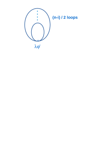
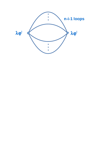
$\Gamma_{2}=\sum\limits_{i=0,n-i=2k}^{n}N_{1}D_{1}+\sum\limits_{i=0}^{n-3}N_{2}D_{2}+\mathsf{g}^{2}D_{3}+\ldots$
$N_{1}=\frac{\lambda}{n!}C_{i}^{n}C_{2}^{n-i},~{}N_{2}=(\frac{\lambda}{n!})^{2}\frac{(n-i)!}{2}(C_{i}^{n})^{2}$

Figure 1: Diagrams contributing to $\Gamma_{2}(\varphi,G)$ up to $\lambda^{2}$ and $\mathsf{g}^{2}$ order of model (2.1). If self-interaction of $\Phi$ is not monomial, similar diagrams with different values of $n$ weighted by the amplitude of monomial terms in the potential must be added to $\Gamma_{2}(\varphi,G)$.

2.2.2 Propagators

Using symmetric and antisymmetric propagators defined in Appendix B and equations (2.18), evolution equations of these propagators [52, 44, 53] for the three fields of the model are obtained as:

$$\biggl{[}\frac{1}{\sqrt{-g}}{\partial}_{\mu}(\sqrt{-g}g^{\mu\nu}{\partial}_{\nu})+M_{i}^{2}(x)\biggr{]}~{}G_{i}^{F}(x,y) = -\int_{-\infty}^{x^{0}}d^{4}z\sqrt{-g(z)}~{}\Pi_{i}^{\rho}(x,z)~{}G_{i}^{F}(z,y)+$$ (2.25)

$$\int_{-\infty}^{y^{0}}d^{4}z\sqrt{-g(z)}~{}\Pi_{i}^{F}(x,z)~{}G_{i}^{\rho}(z,y)$$

$$\biggl{[}\frac{1}{\sqrt{-g}}{\partial}_{\mu}(\sqrt{-g}g^{\mu\nu}{\partial}_{\nu})+M_{i}^{2}(x)\biggl{]}~{}G_{i}^{\rho}(x,y) = -\int_{y^{0}}^{x^{0}}d^{4}z\sqrt{-g(z)}~{}\Pi_{i}^{\rho}(x,z)~{}G_{i}^{\rho}(z,y)$$ (2.26)

$$M_{\Phi}^{2}(x)=m_{\Phi}^{2}+\frac{\lambda}{(n-1)!}\sum_{j=0}^{[n/2]-1}C^{[n/2]-1}_{j}\varphi^{n-2(j+1)}(x)(G^{F}_{\Phi}(x,x))^{j},\quad M_{X,A}^{2}=m_{X,A}^{2}$$ (2.27)

where $i=X,~{}A,~{}\phi$. In (2.27) $[n/2]$ means the integer part of $n/2$ and $C^{i}_{j}$ is the combinatory coefficient. Effective masses $M_{i},~{}i=X,~{}A,~{}\phi$ include local 2PI corrections. However, as $X$ and $A$ are assumed not to have self-interaction, no local mass correction is induced to their propagators. If the fields of the models have internal symmetries, $G$’s and $\Pi$’s may have internal symmetry indices. In this case, eq. (2.26) applies also to mixed propagators. Here we mostly consider the simpler case of single fields without internal symmetries and only briefly mention the case with internal symmetry. We also ignore species index $i$ when there is no risk of confusion. If we assume that all interactions are switched on at the initial time $t_{0}$, the lower limit of integrals in (2.26) will shift to $t_{0}$. Self-energies $\Pi^{F}$ and $\Pi^{\rho}$ are defined in Appendix B. Symmetric and antisymmetric propagators are suitable for studying the evolution of a quantum system, specially numerically, because the r.h.s. of their evolution equations are explicitly unitary and causal [52, 44].

To proceed with detailed construction of evolution equations, we need to specify 2PI diagrams that contribute to in-in expectation values in (2.24) and self-energy in (2.25) and (2.26). Figs. 2 and 3 show these diagrams. We remark that for interaction (a) in (2.5) a non-zero condensate does not induce a local mass. By contrast it is easy to see that interactions (b) and (c) can be considered as effective mass for $A$ and $\Phi$, respectively. In these cases the mass matrix of fields is not diagonal and the model has an induced $O(2)$ symmetry when condensates are present and in addition to usual loop diagrams, one must consider mixed propagators $G_{AB}$, where $A$ and $B$ are different fields. Like their diagonal counterparts evolution of mixed propagators is ruled by eqs. (2.25) and (2.26), but additional Feynman diagrams [44] including condensate insertion contribute to these equations. However, because the amplitude of induced mass (insertion) is proportional to the coupling, diagrams with mixed propagators have higher perturbative order than their single-field counterparts.

$D_{4}$	$D_{5}$	$D_{6}$
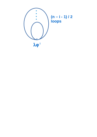
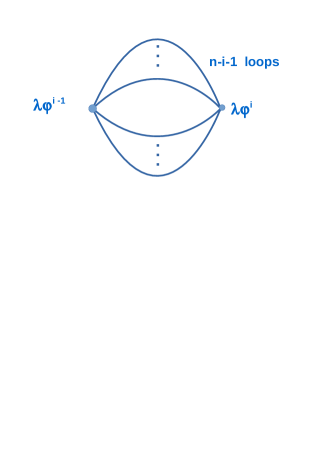
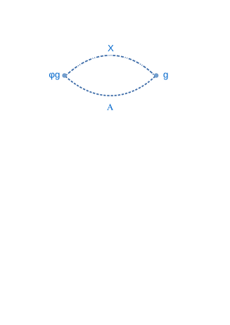
$\frac{\partial\Gamma_{2}}{\partial\varphi}=\sum\limits_{i=0,n-i=2}^{n-1}iN_{1}D_{4}+2\sum\limits_{i=1}^{n-3}iN_{2}D_{5}+2\mathsf{g}^{2}D_{6}+\ldots$

Figure 2: Diagrams contributing to $\partial\Gamma_{2}(\varphi,G)/\partial\varphi$ up to $\lambda^{2}$ and $\mathsf{g}^{2}$ order. They correspond to correlation functions in (2.24). Coefficients $N_{1}$ and $N_{2}$ are defined in Fig. 1. Diagram $D_{6}$ contributes to $\langle X(x)A(x)\rangle$ in eq. (2.24) and presents contraction of $\varphi(y)X(y)A(y)$ in $\mathsf{g}^{2}$-order correction $\langle X(x)\varphi(y)X(y)A(y)A(x)\rangle$ to this correlation function.

$D_{7}$	$D_{8}$	$D_{9}$
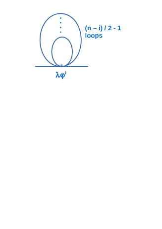
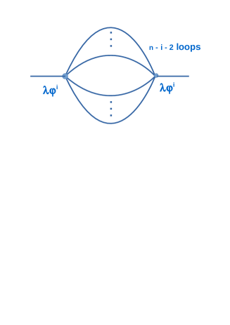
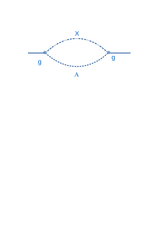
$\frac{\partial\Gamma_{2}}{\partial G_{\phi}}=\sum\limits_{i=0,n-i=2k}^{n-2}\frac{(n-i)N_{1}}{2}D_{7}+\sum\limits_{i=0}^{n-3}(n-i)N_{2}D_{8}+\mathsf{g}^{2}D_{9}\ldots$
$D_{10}$	$D_{11}$
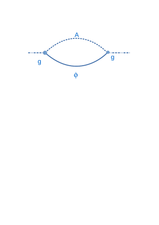
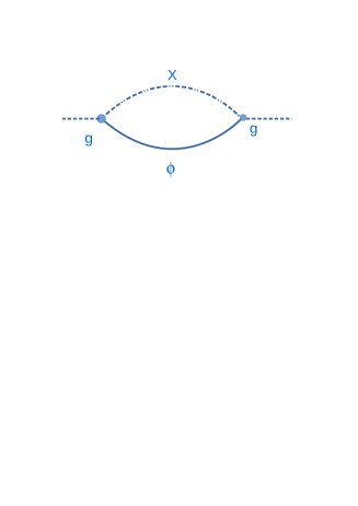
$\frac{\partial\Gamma_{2}}{\partial G_{X}}=\mathsf{g}^{2}D_{10}$	$\frac{\partial\Gamma_{2}}{\partial G_{A}}=\mathsf{g}^{2}D_{11}$

Figure 3: Diagrams contributing to $\partial\Gamma_{2}(\varphi,G)/\partial G_{\phi}$, $\partial\Gamma_{2}(\varphi,G)/\partial G_{X}$, and $\partial\Gamma_{2}(\varphi,G)/\partial G_{A}$, or in other words to self-energies. Coefficients $N_{1}$ and $N_{2}$ are defined in Fig. 1. The tadpole diagrams only contribute to effective mass term (2.27) and do not appear in r.h.s. of equations (2.25) and (2.26).

2.3 Renormalization

Renormalization of 2PI formulation of $\Phi^{n}$ models in Minkowski space is studied in details in [58], with thermal initial state in [59], and that of gauged models in [60]. Numerical simulation of 2PI renormalization using both BPHZ [61] counterterm method and exact renormalization group equation [62, 63] is described in details in [64].

Although significant development on the renormalization of quantum field theories in curved spacetimes is achieved, specially using the method called adiabatic regularization [65, 54], their application to 2PI formalism has been mostly in de Sitter space. For instance, heat kernel [52, 24] and non-perturbative Renormalization Group (RG) flow are used to determine the effect of quantum corrections on the evolution of inflation and scalar perturbations [66] . The exact renormalization group equation is also employed to determine quantum corrected effective potential of inflation [28]. Moreover, the BPHZ counterterm method is used to renormalize this quantity as well as the energy-momentum tensor [67]. Aside from the importance of effective potential for comparison with cosmological observations, it also determines whether at the end of inflation symmetries broken by the inflaton condensate were restored [20].

Application of the Weinberg power counting theorem shows that the model studied here is renormalizable for all the interaction options between $X,~{}A,~{}\Phi$ fields considered in (2.5), and for self-interaction order $n=3~{}\&~{}4$. Although all renormalization techniques lead to finite physical observables and their running with scale, some methods may be more suitable for some applications than others. Notably, adiabatic subtraction is more suitable and straightforward for numerical solution of evolution equations and has been used for calculation of nonequilibrium quantum effects during reheating after inflation [11, 12].

In this method rather than renormalizing effective Lagrangian, which is performed in BPHZ and RG techniques, Green’s functions are renormalized. For renormalizing a n-point Green’s function, the expansion of vacuum Green’s function $G_{vac}$ of the same order (number of points) with respect to expansion rate and its derivatives up to finite terms is subtracted, mode by mode, from bare Green’s function [65, 54, 11]. Propagators are determined at desired perturbative order using the solution of equation (2.25) with r.h.s. put to zero and vacuum initial conditions - corresponding to $|\psi|^{2}=0$ in (D.5). As no analytical solution for evolution equations with an arbitrary $a(t)$ is known, one has to use a WKB expansion [11, 12]. Exact solutions of field equations, when they exist, and WKB approximation and its expansion with respect to $\dot{a}$ and its derivatives are reviewed in Appendix G.

Although the exact expressions of the solutions of evolution equations depend on the initial conditions, which we discuss in detail is Sec. 3, a simple power counting of the integrals in (D.5) shows that they are UV divergent. For $\Phi$ propagators these singularities are generated by the local term in self-energy, which is quadrically divergent, and by 2-vertex diagrams, which have logarithmic UV singularities, see Fig. 3. Self-energy diagrams of $X$ and $A$ are only logarithmically divergent because we assumed $\lambda^{\prime}=0$ in Lagrangian (2.1). Similarly, tadpole and 2-vertex expectation values in the evolution equation of $\Phi$ condensate $\varphi$ are quadrically divergent.

A theorem by Fulling, Sweeny, and Wald (FSW) [69] states that if a singular 2-point Green’s function $G(x,y)$ at $x\rightarrow y$ can be decomposed to smooth functions $u(x,y)$, $v(x,y)$ and $w(x,y)$ in an open neighbourhood on a Cauchy surface such that:

$$G(x,y)=\frac{u(x,y)}{\sigma}+v(x,y)\ln\sigma+w(x,y),\quad\quad\sigma\equiv\frac{1}{2}|x-y|^{2}$$ (2.28)

$$v(x,y)=\sum_{n}v_{n}(x,y)\sigma^{n},\quad\quad w(x,y)=\sum_{n}w_{n}(x,y)$$ (2.29)

where $u$, $v_{n}$ and $w_{n}$ satisfy Hadamard recursion relation, then $G(x,y)$ has the Hadamard form (2.28) everywhere and evolution of Cauchy surface preserves this property. In curved spacetime this theorem assures that the structure of singularities of adiabatic vacuum propagators is preserved during the evolution of fields and geometry.

Power counting of singularities of the effective mass term explained above shows that their singularities are of the same order as those in (2.28). Therefore, $G$ and $G_{vac}$ have the same sort of singularities, and according to FSW theorem subtraction of their divergent terms should lead to a finite and renormalized theory. However, this theorem is proved for 2-point operator valued distributions which satisfy a wave function equation of the form:

$$\biggl{(}D_{\mu}D^{\mu}+M(x)\biggr{)}G(x,y)=I(x,y)$$ (2.30)

where $I(x,y)$ is a smooth external source. Therefore, apriori it cannot be applied to exact propagators in 2PI, which satisfy the integro-differential equations (2.25) and (2.26). On the other hand, we can heuristically and perturbatively consider the integrals on the r.h.s. of (2.25) as an small external source, which depends on second and higher orders of coupling constants. In this case FSW theorem would be applicable, and we can define renormalized propagators as:

$$G_{R}(x,y)=G_{B}(x,y)-G_{vac_{N}}(x,y)$$ (2.31)

where $R$ and $B$ indicate renormalized and bare quantities, respectively. The index $N$ is the adiabatic order in the expansion of vacuum with respect to derivatives of expansion factor. It must correspond to divergence order of the Green’s function. More generally, renormalized expectation value of any operator $\mathcal{O}$ can be formally expressed as:

$$\langle\mathcal{O}\rangle_{R}=\langle\mathcal{O}\rangle_{B}-\langle\mathcal{O}\rangle_{vac,N}$$ (2.32)

where $N$ must correspond to singularity order of $\langle\mathcal{O}\rangle_{B}$. The reason for calling this expression formal is that it does not explicitly show how subdivergences - divergent subdiagrams - are renormalized. Indeed, the method of adiabatic regularization was originally developed for regularization of expectation value of number operator on vacuum state of a free scalar field [70]. Nonetheless, the technique can be applied to interacting models by subtracting adiabatic expansion of a vacuum solution separately for each mode in each loop. This hierarchical subtraction procedure is similar to the addition of counterterms to Lagrangian to remove subdivergences in BPHZ method. For instance, tadpole diagrams $D_{4},~{}D_{7}$ in Figs. 2 and 3 for $n=4$ self-coupling model, which contribute to the effective mass of condensate and propagator, respectively, can be renormalized as:

$$[D_{4}\&D_{7}]_{R}~{}\propto~{}\frac{1}{(2\pi)^{3}}\int dk^{3}e^{-ik.\mathbf{x}}a^{-3/2}[G_{B}(k,t)-|\mathcal{U}^{(2)}_{k}(t)|^{2}]$$ (2.33)

where $G_{B}(k,t)$ is the bare propagator evolving according to eq. (2.25). The function $\mathcal{U}^{(2)}_{k}$, $|\mathcal{U}^{(2)}_{k}|^{2}\equiv G^{(2)}_{vac}(k,t)$ is the adiabatic expansion up to order 2 of the solution of free field equation defined in (3.17). The adiabatic order corresponds to divergence order of $D_{4}$ diagram and the expansion is performed according to expression (G.14). 1-loop diagrams in $D_{2}$, $D_{5}$ and $D_{6}$ are only logarithmically divergent. Therefore, in Fourier space we have to determine subtractions of form $G_{B}(k,t)G_{B}(k,t)-G^{(0)}_{vac}(k,t)G^{(0)}_{vac}(k,t)$, where we have omitted species and path indices. Implementation of this renormalization procedure in numerical calculations is much easier than e.g. abstract counterterms in BPHZ method or variation of dimension in dimensional regularization and renormalization. In any case, diagrams in Figs. 1-3 do not contain any divergent sub-diagram and problem of subdivergence does not arise at perturbation orders considered in this work.

Renormalized condensate $\varphi_{R}$ is obtained by using renormalized expectation values in its evolution equation (2.24) and no additional renormalization would be necessary. From now on we assume that adiabatic renormalization procedure is applied to observables and drop the subscript $R$ when it is not strictly necessary.

2.3.1 Initial conditions for renormalization

In order to fix renormalized mass, self-coupling, and coupling between $X$, $A$, and $\Phi$ we define the following initial conditions:

$$\frac{\delta^{2}\Gamma_{R}(\varphi_{R},G_{R})}{\delta\varphi_{R}^{2}}\biggr{|}_{\varphi_{R}=0,\mu_{0}}=-m^{2}_{R\Phi},\quad\frac{\delta^{n}\Gamma_{R}(\varphi_{R},G_{R})}{\delta\varphi_{R}^{n}}\biggr{|}_{\varphi_{R}=0,\mu_{0}}=-\lambda_{R},\quad\frac{\delta^{2}\Gamma_{R}(\varphi_{R},G_{R})}{\delta(\partial_{\mu}\varphi_{R})\delta(\partial_{\nu}\varphi_{R})}\biggr{|}_{\varphi_{R}=0,\mu_{0}}=g^{\mu\nu}$$

(2.34)

$$\frac{\delta^{3}\Gamma_{R}(\varphi_{R},G_{R})}{\delta G_{R_{\phi}}(x,y)\delta G_{R_{X}}(x,y)\delta G_{R_{A}}(x,y)}\biggr{|}_{\varphi_{R}=0}=\mathsf{g}^{2}_{R}.\quad$$ (2.35)

$$\frac{\delta\Gamma_{R}(\varphi_{R},G_{R})}{\delta G_{R_{X}}(x,x)}\biggr{|}_{\varphi_{R}=0,\mu_{0}}=M_{R_{X}}^{2}(x)=m_{R_{X}}^{2}\quad\quad\frac{\delta\Gamma_{R}(\varphi_{R},G_{R})}{\delta G_{R_{A}}(x,x)}\biggr{|}_{\varphi_{R}=0,\mu_{0}}=M_{R_{A}}^{2}(x)=m_{R_{A}}^{2}.$$ (2.36)

$$\frac{\delta^{3}\Gamma_{R}(\varphi_{R},G_{R})}{\delta\varphi_{R}(x,y)\delta G_{R_{X}}(x,y)\delta G_{R_{A}}(x,y)}\biggr{|}_{\varphi_{R}=0}=\mathsf{g}_{R}.\quad$$ (2.37)

where a renormalization scale $\mu_{0}\ll M_{X}\ll M_{P}$ is assumed. Due to interaction with the condensate, masses and couplings depend on the amplitude of the condensate $\varphi$ and their values at renormalization scale must be defined for a given value of the condensate. The choice of $\varphi=0$ in (2.34)-(2.37) is motivated by the fact that we assume $\varphi(t_{0})=0$, where $t_{0}$ is the initial time in simulations discussed in Sec. 4. Similar to Lagrangian renormalization techniques, a renormalization group equation can be written for adiabatic subtraction method with respect to adiabatic time scale $T\sim 1/\mu_{0}$, which is used for adiabatic expansion, see Appendix G and [65, 54] for more details. Equation (2.37) is a consistency condition for coupling of the classical field $\varphi$ with $X$ and $A$. It is not independent of $XA\Phi$ vertex defined in (2.35) and is included in the renormalization conditions for the sake of completeness.

We remind that the Lagrangian (2.5) is not symmetric with respect to fields $X,~{}A$ and $\Phi$, and there is no mixed propagator in the model. However, if we consider an internal symmetry for each of the three $X,~{}A$ and $\Phi$ fields, the effective Lagrangian will depend on mixed propagators carrying 2 different internal indices. In this case, additional renormalization conditions for mixed propagators and interaction vertices, which must respect symmetries, would be necessary. As in the simulations discussed in Sec. 4 we only consider the simple case of fields without internal symmetry, we do not discuss the case with internal symmetry further. Scalar field models with $O(N)$ symmetry and their renormalization are extensively studied in the literature, see e.g. [67].

In a cosmological context the expansion of the Universe pushes all scales to lower energies. Thus, cutoffs can be considered as time-dependent and correlated with the evolution of the model. This induces more complications in interpretation of results, for instance whether inflation is IR stable and long range quantum correlations are suppressed [16]-[23]. In de Sitter space the symmetry of space allows to write time-dependence of cutoffs as a factor [28] and dependence of quantities on the cutoff can be studied in the same way as in Minkowski space. But in a general FLRW geometry, even in homogeneous case, such a factorization does not occur [35]. Other choices of regulator, for instance explicit dependence of renormalization scale to expansion factor [11], that is replacement of $\mu_{0}$ with $\mu=a(\eta)\mu_{0}$, are also suggested. However, they induce non-trivial effects at IR limit and only in De Sitter space the IR limit can be followed analytically [25, 20, 16, 22].

2.4 Effective energy-momentum tensor and metric evolution

In semi-classical approach to gravity the effective action (2.22) can be used [54, 52] to define an effective energy-momentum tensor $T^{\mu\nu}_{eff}$, which is then used to evolve metric according to Einstein equations or alternatively a modified gravity model [3]. Here we only consider Einstein gravity:

$$G_{\mu\nu}(x)\equiv 8\pi\mathcal{G}~{}T^{\mu\nu}_{eff},\quad\quad T^{\mu\nu}_{eff}\equiv\langle\hat{T}^{\mu\nu}(x)\rangle_{R}=\frac{2}{\sqrt{-g}}\biggl{(}\frac{\partial\Gamma_{R}}{\partial g_{\mu\nu}(x)}\biggr{)}$$ (2.38)

where $G_{\mu\nu}\equiv R_{\mu\nu}-1/2g_{\mu\nu}R$ is the Einstein tensor and the index $R$ means that for this calculation we use the renormalized effective action. From now on we drop this index where this does not induce any confusion. We remind that effective energy-momentum tensor $T^{\mu\nu}_{eff}$ is a classical quantity and as such it must be finite, if the underlying quantum theory is physically meaningful. Thus, no additional regularization or renormalization condition should be imposed on it. By contrast, the exact expression for $\hat{T}_{R}^{\mu\nu}(x)$ with respect to fields of the model is unknown and its bare version may include singularities. Assumption of energy-momentum tensor as a classical effective quantity is in strict contrast to usual approach, in which classical Lagrangian is used to define a quantum energy-momentum operator $\hat{T}^{\mu\nu}(x)$. This field has usually a quartic divergence and must be renormalized. By contrast, in the semi-classical approach (2.38), once quantities in the effective Lagrangian are renormalized, derived quantities such as $T^{\mu\nu}_{eff}$ are finite. However, initial conditions for renormalization defined in (2.34) and (2.35) do not fix the wave-function normalization. In Sec. 3 we show that the initial value of $T^{\mu\nu}_{eff}$, which is necessary for solving Einstein equations, fixes the wave-function renormalization and the ensemble of condensate, propagators, and metric evolution equations can be solved in a consistent manner.

Using (2.22) the energy-momentum tensor is described as:

$$T^{\mu\nu}_{eff}(x)=\frac{2}{\sqrt{-g}}\biggl{\{}\frac{\partial S(\varphi)}{\partial g_{\mu\nu}(x)}+\frac{i}{2}\sum_{i=\Phi,X,A}\biggl{[}\text{tr}\biggl{(}\frac{\partial\ln G_{i}^{-1}}{\partial g_{\mu\nu}(x)}\biggr{)}+\text{tr}\biggl{(}\frac{\partial\mathcal{G}_{i}^{-1}G_{i}}{\partial g_{\mu\nu}(x)}\biggr{)}\biggr{]}+\frac{\partial\Gamma_{2}}{\partial g_{\mu\nu}(x)}\biggr{\}}$$ (2.39)

The first term in (2.39) is the energy-momentum tensor $T^{\mu\nu}_{cl}(\varphi)$ of the classical condensate field $\varphi$:

$$T^{\mu\nu}_{cl}(\varphi)\equiv\frac{2}{\sqrt{-g}}\frac{\partial S(\varphi)}{\partial g_{\mu\nu}(x)}=\partial^{\mu}\varphi\partial^{\nu}\varphi+g^{\mu\nu}V_{eff}(\varphi)-\frac{1}{2}g^{\mu\nu}g^{\rho\sigma}\partial_{\rho}\varphi\partial_{\sigma}\varphi$$ (2.40)

where $V_{eff}$ is the effective interaction potential of condensate in which the bare mass $m$ is replaced by quantum corrected mass $M(x)$. Other terms in (2.39) can be calculated separately as the followings (for the sake of notation simplicity we drop species index):

$$\frac{i}{\sqrt{-g}}\biggl{(}\text{tr}\frac{\partial\ln G^{-1}}{\partial g_{\mu\nu}(x)}\biggr{)} = \frac{i}{\sqrt{-g}}~{}\frac{\partial}{\partial g_{\mu\nu}(x)}~{}\int d^{4}x\sqrt{-g(x)}~{}\int d^{4}y\sqrt{-g(y)}\ln G^{-1}(x,y)\delta^{4}(x,y)$$ (2.41)

$$= -\frac{i}{2}g_{\mu\nu}(x)tr\ln G^{-1}$$

where we used the equality $\partial\sqrt{-g}/\partial g_{\mu\nu}=-g^{\mu\nu}\sqrt{-g}/2$. We notice that the l.h.s. of (2.41) contributes to Einstein equation as a cosmological constant and its value depends on the normalization of wave function, which we discuss in Sec. 3.4. We drop this term from $T_{eff}^{\mu\nu}$ because we show later that it can be included in the wave function renormalization of fields.

The next term in (2.40) can be expanded as:

$$\frac{i}{\sqrt{-g}}\text{tr}\biggl{(}\frac{\partial\mathcal{G}^{-1}G}{\partial g_{\mu\nu}(x)}\biggr{)} = \frac{-1}{\sqrt{-g}}\frac{\partial}{\partial g_{\mu\nu}(x)}\int d^{4}x^{\prime}\sqrt{-g(x^{\prime})}\int d^{4}y^{\prime}\sqrt{-g(y^{\prime})}\biggl{[}D^{\rho}D_{\rho}^{x^{\prime}}+M^{2}(x^{\prime})\biggr{]}\delta^{4}(x^{\prime},y^{\prime})G(x^{\prime},y^{\prime})$$

$$= \frac{-1}{\sqrt{-g(x)}}\frac{\partial}{\partial g_{\mu\nu}(x)}\int d^{4}x^{\prime}\sqrt{-g(x^{\prime})}\biggl{[}D^{\rho}D_{\rho}^{x^{\prime}}+M^{2}(x^{\prime})\biggr{]}G(x^{\prime},y^{\prime}=x^{\prime})$$

where we have used the definition of $\mathcal{G}^{-1}$ in (2.9). As expected, if non-local 2PI quantum corrections are neglected, $G^{-1}\rightarrow\mathcal{G}^{-1}$, the integrand in the second line of (LABEL:enermom2mid) becomes $\delta^{4}(x^{\prime},y^{\prime}=x^{\prime})$, and the integral becomes a constant, which can be added to vacuum/wave function renormalization.

Using:

$$\biggl{[}\frac{\partial}{\partial g_{\mu\nu}},D_{\rho}\biggr{]}=\biggl{[}\frac{\partial}{\partial g_{\mu\nu}},D^{\rho}\biggr{]}=0$$ (2.43)

the functional derivative in the second line of (LABEL:enermom2mid) is determined as:

$$\frac{i}{\sqrt{-g}}\text{tr}\biggl{(}\frac{\partial\mathcal{G}^{-1}G}{\partial g_{\mu\nu}(x)}\biggr{)}=\frac{1}{2}\biggl{[}g_{\mu\nu}\biggl{(}D^{\rho}D_{\rho}+M^{2}\biggr{)}G(x,x)-D_{\mu}D_{\nu}G(x,x)-D_{\nu}D_{\mu}G(x,x)\biggr{]}$$ (2.44)

The last term of (2.39) is the contribution of 2PI in the energy-momentum tensor and is model dependent. It is determined from derivatives of diagrams in Fig. 1, and up to $\lambda^{2}$ and $\mathsf{g}^{2}$ order has the following explicit expression:

$$\frac{2i}{\sqrt{-g}}\frac{\partial\Gamma_{2}}{\partial g_{\mu\nu}(x)} = ig_{\mu\nu}\biggl{[}(\frac{-i\lambda}{n!})\sum_{i=0}^{[n/2]}C^{n}_{2i}C^{2i}_{2}G^{i}(x,x)\varphi^{n-2i}+$$ (2.45)

$$(\frac{-i\lambda}{n!})^{2}\sum_{i=0}^{n-2}(C^{n}_{i})^{2}(n-i)!\oint d^{4}y\sqrt{-g(y)}\varphi^{i}(x)\varphi^{i}(y)G^{n-i}(x,y)\biggr{]}+$$

$$(i\mathsf{g})^{2}g_{\mu\nu}\oint d^{4}y\sqrt{-g(y)}G_{\Phi}(x,y)~{}G_{X}(x,y)~{}G_{A}(x,y)+$$

$$(i\mathsf{g})^{2}g_{\mu\nu}\oint d^{4}y\sqrt{-g(y)}\varphi(x)\varphi(y)~{}G_{X}(x,y)~{}G_{A}(x,y)+\ldots$$

where $\oint$ means closed time path and $G^{>}$ and $G^{<}$ are used on advance and reverse time branches, respectively. We assume equal condensates on the two branches. Thus, $\varphi^{-}=\varphi^{+}$.

Finally, the renormalized energy-momentum tensor is be explicitly written as:

$$T^{\mu\nu}_{eff} = T^{\mu\nu}_{cl}(\varphi_{R})+\frac{1}{2}\sum_{i=\Phi,X,A}\biggl{[}g^{\mu\nu}\biggl{(}g^{\rho\sigma}D_{\rho}D_{\sigma}+M_{i}^{2}(x)\biggr{)}G^{F}_{Ri}(x,x)-\biggl{(}D^{\mu}D^{\nu}G^{F}_{Ri}(x,x)+D^{\nu}D^{\mu}G^{F}_{Ri}(x,x)\biggr{)}\biggr{]}+$$ (2.46)

$$\frac{2i}{\sqrt{-g}}\frac{\partial\Gamma_{2}[G_{B}]}{\partial g_{\mu\nu}(x)}$$

To get a physical insight into the terms in (2.46) we write $T_{eff}^{\mu\nu}$ as a fluid. The energy-momentum tensor of a classical fluid is defined as:

$$T^{\mu\nu}=(\rho+p)u^{\mu}u^{\nu}-g^{\mu\nu}p+\Pi^{\mu\nu},\quad\quad g_{\mu\nu}\Pi^{\mu\nu}\equiv 0,\quad\quad u_{\mu}u_{\nu}\Pi^{\mu\nu}\equiv 0,\quad\quad u^{\mu}u_{\mu}\equiv 1$$ (2.47)

It is straightforward to obtain following relations for Lorentz invariant density $\rho$, pressure $P$ and for shear tensor $\Pi^{\mu\nu}$:

$$\rho=u_{\mu}u_{\nu}T^{\mu\nu}\quad\quad T\equiv g_{\mu\nu}T^{\mu\nu}=\rho-3p$$ (2.48)

The unit vector $u^{\mu}$ is arbitrary. It defines the equal-time 3D surfaces and the only condition it must satisfy is $u_{\mu}u^{\mu}=1$. In kinetic theory it is conventionally chosen in the direction of the movement of the fluid.

Definitions (2.47) and (2.48) leads to the following expressions for fluid description of a classical scalar field with potential $V$:

$$\rho^{(cl)}_{\varphi}=\frac{1}{2}\partial_{\mu}\varphi\partial^{\mu}\varphi+V(\varphi),\quad\quad p^{(cl)}_{\varphi}=\frac{1}{2}\partial_{\mu}\varphi\partial^{\mu}\varphi-V(\varphi),\quad\quad\Pi^{(cl)}_{\varphi}=0.$$ (2.49)

After decomposing the effective energy-momentum tensor (2.46) as a fluid we find $\rho$, $p$ and $P^{\mu\nu}$ as the followings:

$$\rho = \rho^{(cl)}_{\varphi}+\sum_{i=\Phi,X,A}\frac{1}{2}\biggl{[}(g^{\rho\sigma}D_{\rho}D_{\sigma}+M_{i}^{2}(x))G^{F}_{i}(x,x)-(u^{\rho}u^{\sigma}D_{\rho}D_{\sigma}+u^{\sigma}u^{\rho}D_{\sigma}D_{\rho})G^{F}_{i}(x,x)\biggr{]}+$$ (2.50)

$$\frac{2i}{\sqrt{-g}}u_{\rho}u_{\sigma}\frac{\partial\Gamma_{2}}{\partial g_{\rho\sigma}}$$

$$p = p^{(cl)}_{\varphi}+\sum_{i=\Phi,X,A}\frac{1}{2}\biggl{[}\frac{1}{3}(g^{\rho\sigma}-u^{\rho}u^{\sigma})(D_{\rho}D_{\sigma}+D_{\sigma}D_{\rho})G^{F}_{i}(x,x)-[g^{\rho\sigma}D_{\rho}D_{\sigma}+M_{i}^{2}(x)]G^{F}_{i}(x,x)\biggr{]}+$$ (2.51)

$$\frac{2i}{3\sqrt{-g}}(u_{\rho}u_{\sigma}-g_{\rho\sigma})\frac{\partial\Gamma_{2}}{\partial g_{\rho\sigma}}$$

$$\Pi^{\mu\nu} = \sum_{i=\Phi,X,A}\frac{1}{2}\biggl{\{}(D_{\rho}D_{\sigma}+D_{\sigma}D_{\rho})G^{F}_{i}(x,x)\biggl{[}u^{\mu}u^{\nu}(\frac{4}{3}u^{\rho}u^{\sigma}-\frac{1}{3}g^{\rho\sigma})-\frac{g^{\mu\nu}}{3}(u^{\rho}u^{\sigma}-g^{\rho\sigma})-g^{\rho\mu}g^{\sigma\nu}\biggr{]}\biggr{\}}+$$ (2.52)

$$\frac{2i}{\sqrt{-g}}\biggl{\{}\frac{\partial\Gamma_{2}}{\partial g_{\mu\nu}}-\biggl{[}u^{\mu}u^{\nu}(\frac{4}{3}u_{\rho}u_{\sigma}-\frac{1}{3}g_{\rho\sigma})-\frac{g^{\mu\nu}}{3}(u_{\rho}u_{\sigma}-g_{\rho\sigma})\biggr{]}\frac{\partial\Gamma_{2}}{\partial g_{\rho\sigma}}\biggr{\}}$$

where $V=V_{eff}$ is used in (2.49) which defines $\rho^{(cl)}_{\varphi}$ and $p^{(cl)}_{\varphi}$ for the condensate. The terms $(g^{\rho\sigma}D_{\rho}D_{\sigma}+M_{i}^{2}(x))G^{F}_{i}(x,x)$ in (2.50-2.52) can be replaced by the r.h.s. of (2.25). Therefore, if 2PI quantum corrections are neglected, these terms would be null. As expected, the shear $\Pi^{\mu\nu}$ is a functional of $G_{i}(x,x)$ and is non-zero only when quantum corrections are taken into account. In (2.52) the terms in the curly brackets are due to 1PI and 2PI quantum corrections, respectively.

Despite unusual appearance of the above expressions for $\rho$ and $p$ they are consistent with fluid formulation when 2PI corrections are neglected. To see this, consider the case of a relativistic fluid, that is when $M(x)\rightarrow 0$ and the condensate $\varphi=0$. In this case the contribution of different fields in (2.50-2.52) can be separated and application of (2.25) to these equations shows that $w\equiv p/\rho=1/3$ and $\Pi^{\mu\nu}=0$ for each field component with $M(x)\rightarrow 0$, as expected for a relativistic classical fluid of particles. If $M(x)\neq 0$ in a homogeneous universe with small perturbations at zero order $n^{\mu}=(1,0,0,0)$ and contribution of the first term in (2.51) is zero and we find $p\rightarrow 0$ when quantum corrections generated by interaction between fields are neglected.

If we neglect 2PI terms, $u^{\mu}$ can be different for each component. For instance, it can be chosen such that space components vanish in a homogeneous universe. This choice is suitable when components are studied or observed separately. Alternatively, the same $u^{\mu}$ can be used for all components. It is proved that in multi-field classical models of inflation such a choice leads to adiabatic evolution of superhorizon modes in Newtonian gauge [72]. We notice that due to the interaction between fields - more precisely the term proportional to $\partial\Gamma_{2}/\partial g_{\rho\sigma}$ - it is not possible to define density and pressure separately for each species, unless we neglect 2PI corrections.

Comparison of expressions (2.50) and (2.51) with $\rho_{\varphi}$ and $p_{\varphi}$ shows that not all the term induced by interactions can be considered as an effective potential, which contributes in $\rho$ and $P$ with opposite sign. Although some of 1PI terms in $\rho$ and $p$ behave similar to a classical potential, others - including 2PI corrections which contain integrals and are non-local - do not follow the rule of a classical potential. Therefore, an effective classical scalar field description cannot present full quantum corrections, even if we neglect the shear - the viscosity - term. In addition, the contribution of species without a condensate is, as expected, a functional of their propagators and its expression is not similar to a simple fluid with $p~{}\propto~{}\rho^{\alpha}$. Thus, $T_{eff}^{\mu\nu}$ cannot be even phenomenologically described by a fluid. Of course, we can always consider the effective action (2.22) and its associated effective energy-momentum tensor (2.46) as a phenomenological classical model. But, such a model has very little similarity with bare Lagrangian of the underlying quantum model described in (2.2-2.5). This observation highlights difficulties and challenges of deducing the physics of early Universe from cosmological observations, which in a large extend reflect only classical gravitational effect of quantum processes. Specifically, the effect of quantum corrections can smear contribution of the classical $\rho_{\varphi}$ and $p_{\varphi}$, which reflect the structure of classical Lagrangian. Therefore, conclusions about underlying inflation models by comparing CMB observations with predictions of models treated classically or with incomplete quantum corrections should be considered premature. See also simulations in [73, 74] which show the backreaction of quantum corrections and their role in the formation of spinodal instabilities in natural inflation models, even when only local quantum corrections are considered. Nonetheless, constraints that CMB observations impose on the amplitude of tensor modes generated by $\Pi^{\mu\nu}$ and measurement of the power spectrum properties should be considered in the selection of parameters of any candidate quantum model of the early Universe. See also Sec. 4 for more discussion about these issues.

2.4.1 Fixing metric gauge

To proceed to solving evolution equations of the model, either analytically or numerically, we must choose an explicit description for the metric in a given gauge. We consider a homogeneous flat FLRW metric for the background geometry and add to it both scalar and tensor fluctuations that subsequently will be truncated to linear order:

$$ds^{2}=a^{2}(\eta)(1+2{\boldsymbol{\psi}})d\eta^{2}-a^{2}(\eta)[(1-2{\boldsymbol{\psi}})\delta_{ij}+h_{ij}]dx^{i}dx^{j},\quad\quad dt=ad\eta$$ (2.53)

where $t$ and $\eta$ are comoving and conformal times, respectively. Explicit expression of connection for this metric is given in Appendix F. This parametrization contains one redundant degree of freedom and does not completely fix the gauge. Nonetheless, it has the advantage of containing both scalar and tensor perturbations and can be easily transformed to familiar Newtonian and conformal gauges. The redundant degree of freedom can be removed from final results by imposing a constraint on $h_{ij}$ and ${\boldsymbol{\psi}}$. For instance, if $h_{ij}=0$, this metric takes the familiar form of Newtonian gauge for scalar perturbations when anisotropic shear is null. If $h_{ij}\propto\delta_{ij}$, the metric gets the general form of Newtonian gauge with two scalar potentials ${\boldsymbol{\psi}}$ and $\upphi\equiv{\boldsymbol{\psi}}-h/6$, where $h\equiv\delta^{ij}h_{ij}$. If in addition ${\boldsymbol{\psi}}=h=0$, the metric becomes homogeneous in conformal gauge form.

For solving evolution equations either analytically - which in the case of the model described here is not possible - or numerically, it is preferable to scale the condensate and propagators such that their evolution equations (2.24), (2.25) and (2.26) depend only on the second derivative with respect to conformal time $\eta$. It is straightforward to show that for the metric (2.53) the following scaling changes the evolution equations of condensate and propagators to the desired from:

$$\frac{1}{\sqrt{-g}}{\partial}_{\mu}\biggl{(}\sqrt{-g}g^{\mu\nu}{\partial}_{\nu}\Xi(x)\biggr{)}+M^{2}(x)\Xi(x)=\text{\color[rgb]{0,0,1} [interaction and quantum corrections]}$$ (2.54)

$$\Xi_{\chi}(x)\equiv a(1-2{\boldsymbol{\psi}}+\frac{h}{4})~{}\Xi(x)$$ (2.55)

$$\Xi_{\chi}^{\prime\prime}-\frac{1}{1-2{\boldsymbol{\psi}}+\frac{h}{4}}\partial_{i}\biggl{[}\biggl{(}(1+\frac{h}{2})\delta^{ij}+h^{ij}\biggr{)}\partial_{j}\biggl{(}\frac{\Xi_{\chi}}{1-2{\boldsymbol{\psi}}+\frac{h}{4}}\biggr{)}\biggr{]}+$$

$$\hskip 42.67912pt\biggl{[}a^{2}M^{2}(x)(1+2{\boldsymbol{\psi}})-\biggl{(}\frac{a^{\prime\prime}}{a}(1-2{\boldsymbol{\psi}}-\frac{h}{4})-4\frac{a^{\prime}}{a}({\boldsymbol{\psi}}^{\prime}-\frac{h^{\prime}}{8})-2({\boldsymbol{\psi}}^{\prime\prime}-\frac{h^{\prime\prime}}{8})\biggr{)}\biggr{]}\Xi_{\chi}=$$

$$\hskip 42.67912pta^{3}(1-\frac{h}{4})\text{\color[rgb]{0,0,1} [interaction and quantum corrections]}$$ (2.56)

where $\Xi$ is any of propagators or the condensate with quantum corrected mass $M(x)$. From now on prime means derivative with respect to conformal time $\eta$. When $\Xi$ is a propagator, it depends on two spacetime coordinates, but differential operators are applied only to one of them. Thus, in (2.54) the dependens on coordinates of the second point is implicit. Interaction and quantum correction terms in the r.h.s. of (2.56) are the same as ones in (2.54) (with respect to unscaled variable $\Xi$). The last arbitrary degree of freedom in metric (2.53) can be chosen to simplify (2.56) without loosing the generality at linear order. For instance, if we choose ${\boldsymbol{\psi}}=h/8$ the evolution equation becomes:

$$\Xi_{\chi}^{\prime\prime}-\partial_{i}\biggl{[}\biggl{(}(1+\frac{h}{2})\delta^{ij}+h^{ij}\biggr{)}\partial_{j}\Xi_{\chi}\biggr{]}+\biggl{[}a^{2}M^{2}(x)(1+\frac{h}{4})-\frac{a^{\prime\prime}}{a}\biggr{]}\Xi_{\chi}=$$

$$\quad\quad a^{3}(1-\frac{h}{4})\text{\color[rgb]{0,0,1} [interaction and quantum correction terms]}$$ (2.57)

The presentation of scaled solution of field equation for linearized Einstein equations is for the sake of completeness of discussions and for future use, because in the simulations presented in Sec. 4 we only use a homogeneous background metric.

3 Initial conditions

To solve semi-classical Einstein equation (2.38) we need evolution of effective energy-momentum tensor $T_{eff}^{\mu\nu}$, which depends on the propagators $G_{i}(x,y),i\in\Phi,~{}X,~{}A$ and the condensate field $\varphi(x)$. Evolution of these quantities is governed by a system of second order differentio-integral equations needing two initial or boundary conditions for each equation. This is in addition to the initial state density which appears in the generating functional $\mathcal{Z}$, because the state of the system at initial time $t_{-0}$ does not give any information about that of $t_{+0}$ in Schrödinger or interaction picture or evolution of operators in Heisenberg picture. In addition, initial conditions for evolution equations of propagators and condensate(s) in a multi-component model are not independent from each others and their consistency must be respected.

The model formulated in the previous sections is independent of the cosmological epoch to which it may be applicable. However, for fixing initial or boundary conditions we have to take into account physical conditions of the Universe at the epoch in which this model and its constituents are supposed to be switched on. Two epochs are of special interest: (pre)-inflation; and epoch of the formation of the component which may play the role of dark energy at present. These two eras may be the same if dark energy is a leftover of inflationary epoch, otherwise different conditions may be necessary for each. In the following subsections we first describe physically interesting initial quantum states for the model. Then, we specify initial conditions for solutions of evolution equations. Explicit description of constraints used for the determination of initial conditions and their solutions are described in Appendix H.

A word is in order about the initial conditions for bare and adiabatic vacuum Green’s functions, because they are primary rather than derived quantities which their evolution is implemented in the numerical simulations. Initial conditions for these functions are arbitrary and different conditions are equivalent to performing a Bogoliubov transformation on creation and annihilation operators. Only initial conditions for renormalized quantities are physically meaningful, lead to observable effects, and must respect observational constraints.

3.1 Density matrix of initial state

Our main purpose in studying the model (2.1) is to learn how the light fields $\Phi$ and $A$ are created from the decay of the heavy field $X$ and how they evolve to induce an accelerating expansion. Therefore, it is natural to assume a vacuum state for $\Phi$ and $A$ at initial time $t_{0}$. The initial state of $X$ can be more diverse. Physically motivated cases are Gaussian, double Gaussian, and free thermal states. The only difference between the first and the second case is the choice of cosmological rest frame. The last case is motivated by hypothesis of a thermal early Universe and the assumption that interaction of $X$ with other fields is switched on at $t_{0}$. As we discussed earlier, both a Gaussian and a free thermal states are Gaussian [57, 41]. We remind that as it is assumed that interactions are switched on at $t_{0}$, $X$ is initially a free field. Consequently, the contribution of its density matrix can be included in 1-point and 2-point correlations and no additional Feynman diagram is needed.

Simulations discussed in Sec. 4 are performed in several steps to prevent exponential increase of numerical errors. The initial state of $\Phi$ and $A$ in intermediate simulations is not any more vacuum and due to interactions the initial state of the system may be non-Gaussian. However, considering the large mass and small coupling of $X$ and $A$, a Gaussian or free thermal initial states for both seem a good approximation. In this case, their density functional $F$ do not change the effective action. However, a non-zero condensate component needs special care. For this reason in the next subsection we calculate elements of matrix density for a condensate state.

3.1.1 Density matrix of coherent states

Following the decomposition (2.7), the state of a scalar can be factorized to $|\Psi\rangle=|\Psi_{C}\rangle\otimes|\Psi_{NC}\rangle$ where $|\Psi_{C}\rangle$ is a condensate state and $|\Psi_{NC}\rangle$ is non-condensate consisting of quasi-free particles. There is no general description for a condensate state, but special cases are known. A physically interesting example of known condensate states, which has been also realized in laboratory [75], is a Glauber coherent state[76]. See also [77] for a review of other coherent states and their applications. The Glauber coherent state is defined as an eigen state of annihilation operator:

$$a_{k}|\Psi_{C}\rangle = C_{k}|\Psi_{C}\rangle$$ (3.1)

$$|\Psi_{C}\rangle \equiv e^{-|C_{k}|^{2}/2}e^{Ca_{k}^{\dagger}}|0\rangle=e^{-|C|^{2}/2}\sum_{i=0}^{\infty}\frac{C_{k}^{i}}{i!}(a_{k}^{\dagger})^{i}|0\rangle$$ (3.2)

It can be generalized to a superposition of condensates of different modes:

$$|\Psi_{GC}\rangle\equiv\int d^{3}kA_{k}e^{C_{k}a_{k}^{\dagger}}|0\rangle=\int d^{3}kA_{k}\sum_{i=0}^{\infty}\frac{C_{k}^{i}}{i!}(a_{k}^{\dagger})^{i}|0\rangle$$ (3.3)

If the support of mode $k$ is discrete, the integral in (3.3) is replaced by a sum. A condensate may be also a combination of condensates of different fields or modes:

$$|\Psi_{mGC}\rangle\equiv\prod_{i}\int d^{3}k_{i}A_{k_{i}}e^{C_{k_{i}}a_{k_{i}}^{\dagger}}|0\rangle=\prod_{i}\int d^{3}k_{i}A_{k_{i}}\sum_{j=0}^{\infty}\frac{C_{k_{i}}^{j}}{j!}(a_{k_{i}}^{\dagger})^{j}|0\rangle$$ (3.4)

where $i$ runs over the set of fields.

It is proved that if a density operator commutes with number operator, its elements over field eigen states have a Gaussian form [57]. However, coherent states are neither eigen states of field operator $\hat{\Phi}$ nor number operator $\hat{N}$. In fact they are explicitly a superposition of states with any number of particles. Elements of density matrix operator $\varrho_{GC}$ of the coherent state $|\Psi_{GC}\rangle$ can be expanded as:

$$\langle\Phi^{\prime}|\varrho_{GC}|\Phi\rangle=\langle\Phi^{\prime}|\int d^{3}k^{\prime}A^{*}_{k^{\prime}}e^{C^{*}_{k^{\prime}}u^{*-1}_{k^{\prime}}\int d^{3}ye^{-ik^{\prime}y}\hat{\phi}^{+}(y)}|0\rangle\langle 0|\int d^{3}kA_{k}e^{C_{k}u^{-1}_{k}\int d^{3}xe^{ikx}\hat{\phi}^{-}(x)}|\Phi\rangle$$ (3.5)

Because $\hat{\phi}^{-}(x)|0\rangle=0$ and $\langle 0|\hat{\phi}^{+}(x)=0$, we can replace $\hat{\phi}^{-}$ and $\hat{\phi}^{+}$ in (3.5) with $\hat{\phi}$ and apply a normal ordering operator $::$ to each factor. Then, using Wick theorem $:\hat{A}\hat{B}:~{}\equiv~{}\hat{A}\hat{B}-\langle 0|\hat{A}\hat{B}|0\rangle I$, we find:

$$\langle\Phi^{\prime}|\varrho_{GC}|\Phi\rangle = \phi_{0}\phi^{{}^{\prime}*}_{0}\int d^{3}k^{\prime}A^{*}_{k^{\prime}}e^{C^{*}_{k^{\prime}}u^{*-1}_{k^{\prime}}\int d^{3}ye^{-ik^{\prime}y}\phi^{\prime}(y)}\int d^{3}kA_{k}e^{C_{k}u^{-1}_{k}\int d^{3}xe^{ikx}\phi(x)}-$$ (3.6)

$$\langle 0|\int d^{3}k^{\prime}A^{*}_{k^{\prime}}e^{C^{*}_{k^{\prime}}u^{*-1}_{k^{\prime}}\int d^{3}ye^{-ik^{\prime}y}\hat{\phi}(y)}|0\rangle\langle 0|\int d^{3}kA_{k}e^{C_{k}u^{-1}_{k}\int d^{3}xe^{ikx}\hat{\phi}(x)}|0\rangle$$

$$= \phi_{0}\phi^{{}^{\prime}*}_{0}\int d^{3}k^{\prime}~{}e^{\int d^{3}yF^{*}_{k^{\prime}}e^{ik^{\prime}y}\hat{\phi}{{}^{\prime}*}(y)}\int d^{3}k~{}e^{\int d^{3}xF_{k}e^{ikx}\hat{\phi}(x)}-\int d^{3}k|A_{k}|^{2}$$

$$F_{k} \equiv C_{k}u^{-1}_{k}\ln A_{k}$$ (3.7)

where $\phi_{0}$ ($\phi^{\prime}_{0}$) is the zero mode of the decomposition of $|\Phi\rangle~{}(|\Phi^{\prime}\rangle)$ to $n$-particle states $|n\rangle~{}\forall~{}n\in\mathbb{Z}$ and $\phi_{k}$ is the 3D Fourier transform of configuration field $\phi$. The last term in (3.6) is the contribution of vacuum, that is when $C_{k}\rightarrow 0~{}\forall k$. It is a constant and can be included in the normalization of wave function, which we fix later in this section.

Insertion of (3.6) in (2.11) gives the generating functional for a system initially in state $|\Psi_{GC}\rangle$:

$$\mathcal{Z}(J_{a},K_{ab};\varrho) \equiv e^{iW[J_{a},K_{ab}]}=\int\mathcal{D}\Phi^{a}\mathcal{D}\Phi^{b}\exp\biggl{[}iS(\Phi^{a})+\int d^{4}x\sqrt{-g}J_{a}(x)\Phi^{a}(x)+$$ (3.8)

$$\frac{1}{2}\int d^{4}xd^{4}y\sqrt{-g(x)}\sqrt{-g(y)}\Phi^{a}(x)K_{ab}(x,y)\Phi^{b}(y)\biggr{]}\times$$

$$\int d^{3}k^{\prime}d^{3}k\biggl{[}\Phi^{a*}_{0}\Phi^{b}_{0}\exp\biggl{(}\int d^{3}yF^{*}_{k^{\prime}}e^{-ik^{\prime}y}\Phi^{a}(y)+\int d^{3}xF_{k}e^{ikx}\Phi^{b}(x)\biggr{)}-A^{*}_{k^{\prime}}A_{k}\biggr{]}$$

where branch indices $a,b\in\{+,-\}$. $\Phi_{0}$ and terms in the last line of (3.8) are evaluated at the initial time $t_{0}$. Comparing the contribution of the initial condition with the definition of $F[\Phi]$ in (2.12) and (2.20), it is clear that only $\alpha_{0}$ and $\alpha_{1}$ are non-zero. They can be included in the normalization factor and $J$ current, and do not induce new diagrams to the effective Lagrangian. Nonetheless, (3.8) explicitly shows that as the system is initially in a superposition state, the classical effective Lagrangian is a quantum expectation obtained by summing over all possible states weighed by their amplitude. Extension of these results to $|\Psi_{mGC}\rangle$ is straightforward.

3.2 Initial conditions for solutions of evolution equations

In the study of inflation and dark energy, specially through numerical simulations, it is more convenient to fix initial conditions, that is the value and variation rate of condensates and propagators on the initial equal-time 3-surface rather than boundary conditions at initial and final times. Initial conditions for inflation are extensively discussed in the literature, see e.g. [78, 79, 56] and [68] (for review). As in this toy model there is not essential difference between (pre)-inflation and dark energy era, the same type of initial conditions can be used for both.

We use a Dirichlet-Neumann boundary condition [56, 80, 35]:

$$n^{\mu}\partial_{\mu}{\mathcal{U}}={\mathcal{K}}{\mathcal{U}},\quad\quad g_{\mu\nu}n^{\mu}n^{\nu}=1$$ (3.9)

where $n^{\mu}$ is a unit vector normal to the initial spacelike 3-surface and $\mathcal{U}$ is a general solution of the evolution equation. Assuming a homogeneous, isotropic and spacelike initial surface, $n^{\mu}=(a^{-1},0,0,0)$ in conformal coordinates. We use boundary conditions similar to (3.9) for both condensate and propagators.

Although $\mathcal{K}$ is arbitrary, it must be consistent with the geometry near initial boundary to provide a smooth transition from initial 3-surface [56, 68]. For instance, if we want that for $t\rightarrow t_{0}$ modes approach to those of a free scalar field in flat Minkowski, $\mathcal{K}$ should have a form similar to modes in a static flat space:

$$\mathcal{K}=i\sqrt{\frac{k^{2}}{a^{2}(t_{0})}+M^{2}}=i\omega_{k}$$ (3.10)

where $M$ is the effective mass. In this choice (3.9) is a condition on the flow of energy from initial surface in Minkowski and de Sitter geometry and is called Bunch-Davis initial condition.

The renormalized anti-symmetric propagator must satisfy the condition imposed by field quantization [53]:

$$\partial_{0}G_{R}^{\rho}(\vec{x},,t,\vec{y},t)=\frac{i\delta^{(3)}(x-y)}{g^{00}\sqrt{-g}}$$ (3.11)

At initial time this constraint can be written for mode functions in synchronous gauge as:

$$\biggl{[}\mathcal{U}_{k}^{\rho^{\prime}}(\eta_{0})\mathcal{U}^{\rho*}_{k}(\eta_{0})-\mathcal{U}^{\rho}_{k}(\eta_{0})\mathcal{U}^{\rho*^{\prime}}_{k}(\eta_{0})\biggr{]}_{R}=\frac{-i}{a^{2}(\eta_{0})}$$ (3.12)

where $\mathcal{U}_{k}^{\rho^{\prime}}$ is the derivative of solution $\mathcal{U}^{\rho}_{k}$ of the free field equation (G.1) with respect to conformal time $\eta$ at $\eta=\eta_{0}$. The bracket and index $R$ means that this constraint is applied after subtraction of adiabatic expansion of vacuum, which makes the propagator finite. The contribution of fields in the energy-momentum tensor imposes a constraint on $G^{F}_{R}$, see Sec. 3.3. It can be used as the second condition for fixing integration constants for these propagators.

3.2.1 Initial conditions for propagators

In what concerns the fields of the toy model, the initial conditions should reflect the absence of $A$ and $\Phi$ particles and $\varphi$ condensate at time $t_{0-}$ and their production by decay of $X$ at $t_{0+}$. Due to this interaction an initial condition of type (3.9) must depend on the solutions of field equations for all the constituent and the constant $\mathcal{K}$ includes production/decay rate of one species from/to another. Therefore, a boundary condition for the derivative of propagators similar to (3.9) which reflects these properties can be defined as the following:

$$n^{\mu}\partial_{\mu}G^{F}_{i}=\sum_{j\in\{X,A,\Phi\}}{\mathcal{K}}_{ij}G^{F}_{j}$$ (3.13)

In general ${\mathcal{K}}_{ij}$ depends on $\vec{x}$ and $\vec{y}$, but if we assume that interactions are switched on at time $\eta_{0+}$, initially propagators are free and both $G_{i}$’s and ${\mathcal{K}}_{ij}$ depend only on $\vec{x}-\vec{y}$. In addition, interpretation of propagators as expectation value of particle number means that for the model discussed here there is a relation between $G_{i}$’s and ${\mathcal{K}}_{ij}$ modes in the Fourier space. Notably, in interaction model (a) in (2.5) momentums of decay remnants are determined uniquely from momentum of decaying particle. In this case, when (3.13) is written in momentum space, convolutions (in momentum space) in the r.h.s. become simple multiplications:

$${G^{\prime}}^{F}_{i}(k) = \sum_{j\in\{X,A,\Phi\}}\int d^{3}p~{}{\mathcal{K}}_{ij}(\vec{k}-\vec{p})G^{F}_{j}(\vec{p})=\sum_{j\in\{X,A,\Phi\}}{\mathcal{K}}_{ij}(\vec{k})G^{F}_{j}(\vec{p}(k))$$ (3.14)

$${\mathcal{K}}_{ij}(k) = {\mathcal{K}}_{i}^{vac}(k)\delta_{ij}+\Gamma_{ij}(p(k))$$ (3.15)

where we have assumed $n^{\mu}=(a^{-1},0,0,0)$ in homogeneous conformal coordinates. The coefficient ${K}_{i}^{vac}$ presents the choice of boundary condition for the vacuum. Here we only consider Bunch-Davis vacuum defined in (3.10). The constant $\Gamma_{ij}$ is the decay width of $j$ to $i$ if $\Gamma_{ij}<0$, and production rate of $i$ from $j$ if $\Gamma_{ij}>0$ [81]. The function $p(k)$ is determined from kinematic of decay/production of $i$ to/from $j$. Under the assumption of initial vacuum state for $\Phi$ and $A$, only $\Gamma_{X\Phi}$ and $\Gamma_{XA}$ contribute to initial conditions. For model (a) in (2.5) $\Gamma_{X\Phi}=\Gamma_{XA}=\Gamma_{X}$, where $\Gamma_{X}$ is the total decay width of $X$ particles. We can use perturbative in-out formalism to determine decay rates at initial time - even in presence of a condensate - because in the infinitesimal time interval of $[t_{0},~{}t_{0}\textdiv\epsilon$ where these rates are needed the system can be considered as quasi-static. This setup and its purpose is very different from effective dissipation rates calculated e.g. in [43], which are time dependent and their purpose is to present 2PI quantum corrections in an effective evolution equations for condensates and cosmological matter fluctuations.

Alternatively we can use the following equation as an initial condition:

$${G^{\prime}}^{F}_{i}(k)=\sum_{j\in\{X,A,\Phi\}}\int d^{3}p~{}{\mathcal{K}}_{ij}(\vec{k}-\vec{p})G^{F}_{j}(\vec{p})={\mathcal{K}}_{i}^{vac}(k)G^{F}_{i}(k)+\Upsilon_{i}(k)\quad i\in\{X,A,\Phi\}$$ (3.16)

where $\Upsilon(k)$ is an external source which must be decided from properties of the model. For instance, in the model (a) if the self-coupling of the light scalar field $\Phi$ is much larger than its coupling to $X$, we can assume that $\Phi$ particles produced from decay of $X$ in the interval $(t_{-0},t_{+0})$ interact with each other and at $t_{+0})$ all memory about their production is lost and particles are distributed according to distribution $\Upsilon_{i}(k)$, which its normalization is determined such that the total energy density of $\Phi$ is equal to the energy transferred to this field from decay of $X$ (we neglect the backreaction). This choice of boundary condition is specially interesting for numerical simulations because it allows to study all the fields in the model in the same range of momentum space. By contrast, in (3.14) the range of $k$ and $p$ for modes with largest amplitudes can be very different if there are large mass gaps between particles. The disadvantage of (3.16) is that it adds a new arbitrary distribution, namely $\Upsilon_{i}(k)$ to the model. Nonetheless, the assumption of the loss of memory due to many scattering means that $\Upsilon_{i}(k)$ can be well approximated by a Gaussian distribution with zero mean value in the frame where initial distribution of $X$ particles has a zero mean value. Its standard deviation, however, remains arbitrary, and apriori can be larger than the standard deviation of momentum distribution of $X$ particles.

A general solution of field equations can be written as:

$$\mathcal{U}_{k}=a^{-1}(c_{k}U_{k}+d_{k}V_{k})$$ (3.17)

where $U_{k}$ and $V_{k}$ are two independent solutions for mode $k$. We have divided the r.h.s. of (3.17) by $a(\eta)$ because solutions $U_{k}$ and $V_{k}$ for free fields are usually obtained for scaled function $\Xi_{\chi}\equiv a\Xi$ where $\Xi$ is any of scalar fields of the model. Solutions of field equation for some spacial geometries and WKB approximation for general case are given in Appendix G. If there is initial correlation/entanglement between fields, it is implicit in the matrix elements of the state (or equivalently density matrix) defined in Appendix C.

From explicit expression of free propagators with respect to independent solutions given in Appendix D it is clear that only the difference between arguments of complex constants $c_{k}$ and $d_{k}$ is observable. In coordinate space this means that free propagators depend on $\vec{x}-\vec{y}$ rather than each coordinate separately, and only 3 initial conditions (for real rather than complex quantities) are enough to fix integration constants. Therefore equations (3.12) and (3.13) can fully fix all the propagators and no additional constraint for defining $c_{k}$ and $d_{k}$ is necessary. However, propagators depend on the normalization of initial quantum state $N$ in (D.7), or equivalently the initial momentum distribution discussed in the next section. It will be fixed by initial conditions imposed on $T^{\mu\nu}_{eff}$ in Sec. 3.3.

Finally, a question must be addressed here: how to calculate decay and scattering rates $\mathcal{K}_{ij}$ consistently ? To determine $\mathcal{K}_{ij}$ with respect to renormalized masses and couplings we need renormalized propagators and condensate, which in turn need the solutions of evolution equations. Thus, the problem seems circular. This issue is not very important for the toy model studied here and its simulations, because there is no observational constraint for parameters and they can be chosen more or less arbitrarily. They only have to be in the physically motivated range and lead to a reasonable cosmological outcome. However, for academic interest it is important to know how one would have to proceed, if observed information about decay width, scattering cross-section, and masses were available. The interdependence of $\mathcal{K}_{ij}$, couplings and masses can be broken if we determine decay width and scattering cross sections at perturbative tree order and assume that initial conditions of renormalization (2.34-2.36) are defined such that $\mathcal{K}_{ij}$ corresponds to observed values at renormalization scale. For model (a) in (2.5) $\Gamma_{X}$ is calculated in [36] and we do not repeat it here.

3.2.2 Initial distribution

In addition to the contribution of density matrix in the generating functional (2.11) the density matrix elements $|\Psi_{k_{1}k_{2}\ldots k_{n}}|^{2}$ (for pure states) are needed for determination of propagators, see (D.1-D.3). As we assume that for both inflation and dark energy, no $\Phi$ or $A$ particle exists at initial time, their contribution in the initial state $|\Psi\rangle$ is simply vacuum. Thus, only the initial state of $X$ particles is non-trivial. In absence of self-interaction for $X$ field in the model (2.1) a free initial state without entanglement is justified and the many-particle wave-function $|\Psi_{k_{1}k_{2}\ldots k_{n}}|^{2}$ can be factorized to 1-particle functions. Moreover, after taking a Wigner transformation, $|\Psi_{k_{1}k_{2}\ldots k_{n}}|^{2}$ can be replaced by a momentum distribution $f_{X}(k,\bar{x},t_{0})$ evaluated at the average coordinate $\bar{x}$ of $X$ particles [57],

1-particle distribution functions of free thermal and single or double Gaussian states discussed in Sec. 3.1 are:

$$f_{X}(k,\bar{x},t_{0})=\begin{cases}\frac{N}{e^{\beta_{\mu}k^{\mu}}-1}&\text{thermal}\\ Ne^{-\frac{|\vec{k}-\vec{k}_{0}|^{2}}{2\sigma^{2}}}&\text{Gaussian}\end{cases}$$ (3.18)

where $\sigma$ is the standard deviation of the Gaussian; $\beta_{\mu}$ is proportional to Killing vector and can be interpreted as covariant extension of inverse temperature [82] In the Gaussian distribution $\vec{k}_{0}$ is a constant 3-momentum presenting the momentum of the center of mass of $X$ particles with respect to an arbitrary reference frame. The factor $N$ is a normalization constant. If at $t_{0}$ the Universe is homogeneous, the distribution $f$ will not depend on $\bar{x}$. If simulations present the era after inflation and $m_{X}\gtrsim 300$ TeV, the distribution of $X$ particles could not be in thermal equilibrium with other species [86]. This is not an issue for our toy model because at the initial time there is no other species. Nonetheless, we preferred to use a Gaussian distribution in our simulations.

Another physically motivated state is a totally entangled state with all particles in one or a few momentum states. This is reminiscent to a Bose-Einstein condensate, but is not a Glauber condensate. If in addition $X$ has internal quantum numbers (symmetries), other type of entanglement would be possible. For instance, in [74] an entanglement between different fields of a multi-field inflation model is considered. It generates a coherent oscillation between scalar fields of the model, which may leave an observable signature on matter fluctuations.

An issue which must be clarified here is the relation between comoving reference frame today - defined as the rest frame of far quasars - and the reference frame in which $f(k,\bar{x},t_{0})$ and other quantities of the model are defined. Although Lorentz invariance assures that final results do not depend on the selection of reference frame, in a multi-component system there can be frames in which the formulation of the model is easier, specially when approximations are involved. Moreover, when theoretical predictions are compared with observations the issue of using the same reference frame for both becomes crucial. If we assume that $X$ particles decay significantly or totally before epochs accessible to observations, today’s comoving frame cannot be directly associated to their rest frame. In this case, it would be more convenient to consider the rest frame of $\varphi$, the condensate of $\Phi$, as the reference frame. When $\varphi$ is identified with classical inflaton field, reheating at the end of inflation is homogeneous in this frame and presumably $\varphi$ frame coincides with the comoving frame today. In addition, if the model studied here is supposed to be a prototype for formation of a quintessence field during or after reheating, the observed homogeneity of dark energy with respect to matter and radiation, which fluctuate, encourages the use of its rest frame as reference.

3.3 Initial condition for geometry

The simplest choice for initial geometry is a homogeneous FLRW metric, that is $\upphi={\boldsymbol{\psi}}=h_{ij}=0$ in metric (2.53). Thus, the metric depends only on the expansion factor $a(\eta)$, which its value at initial time is irrelevant and without loss of generality can be considered to be $a(\eta_{0})=1$. The value of Hubble constant $H\equiv\dot{a}/a$ (or equivalently $\mathcal{H}\equiv aH=a^{\prime}/a$) must be chosen based on the physics of inflation or reheating after inflation, respectively for studying condensation of inflaton or dark energy from decay of the heavy particle $X$.

In a homogeneous FLRW metric only diagonal components of Einstein tensor are nonzero :

$$G_{\alpha}^{\beta^{\prime\prime}}-\delta^{ij}\partial_{i}\partial_{j}G_{\alpha}^{\beta}+2\mathcal{H}G_{\alpha}^{\beta^{\prime}}+M_{\alpha}^{2}(x)a^{2}G_{\alpha}^{\beta}=\text{\color[rgb]{0,0,1} [2PI corrections]}\quad\quad\alpha\in X,A,\Phi\quad\beta\in{F,\rho}$$ (3.19)

$$T^{\eta\eta} = T_{cl}^{\eta\eta}+\sum_{\alpha\in X,A,\Phi}\frac{1}{2a^{4}}\biggl{[}-G_{\alpha}^{F^{\prime\prime}}-\delta^{ij}\partial_{i}\partial_{j}G_{\alpha}^{F}+4\mathcal{H}G_{\alpha}^{F^{\prime}}+M_{\alpha}^{2}(x)a^{2}G_{\alpha}^{F}\biggr{]}+\frac{2i}{\sqrt{-g}}\frac{\partial\Gamma_{2}}{\partial g_{\eta\eta}}$$

$$T^{\eta\eta}_{homo} = \frac{3\mathcal{H}^{2}}{8\pi\mathcal{G}a^{4}},\quad\quad\mathcal{H}\equiv\frac{a^{\prime}}{a}$$ (3.21)

where $T^{\eta\eta}$ is the $00$ component of energy-momentum tensor in homogeneous conformal metric and propagators are evaluated at $(\vec{x},\eta,\vec{y}=\vec{x},\eta)$. According to our assumptions described earlier, at initial time $T_{cl}^{\eta\eta}$, contributions of $A$ and $\Phi$ in the second term of (LABEL:tetaeta), and the last term are all zero.

Spatial components of energy-momentum tensor $T^{ij}$ for homogeneous background metric are:

$$\sum_{\alpha\in X,A,\Phi}T_{\alpha}^{ij}(\eta) = \sum_{\alpha\in X,A,\Phi}\frac{1}{2a^{4}}\biggl{[}-\delta^{ij}(G_{\alpha}^{F^{\prime\prime}}-\mathcal{H}G_{\alpha}^{F^{\prime}}+M_{\alpha}^{2}(x)a^{2}G_{\alpha}^{F})+(\delta^{ij}\delta^{kl}-2\delta^{ik}\delta^{jl})(\partial_{k}\partial_{l}G_{\alpha}^{F}-\delta_{kl}\mathcal{H}G_{\alpha}^{F^{\prime}})\biggr{]}+$$ (3.22)

$$\frac{2i}{\sqrt{-g}}\frac{\partial\Gamma_{2}}{\partial g_{ij}}$$

They do not impose further constraints on the model, but are needed for determination of the equation of state defined as $w\equiv p/\rho$, where $\rho=a^{2}T^{\eta\eta}$ and $P=a^{2}\delta^{ij}T^{ij}/3$. Using Einstein equations $a^{\prime\prime}$, which is necessary for solving field equations, is obtained as:

$$\frac{a^{\prime\prime}}{a}=\frac{4\pi\mathcal{G}}{3}\biggl{\{}a^{2}T_{cl}(\varphi)+\sum_{\alpha\in X,A,\Phi}\biggl{[}G_{\alpha}^{F^{\prime\prime}}-\partial_{i}\partial^{i}G_{\alpha}^{F}+2\mathcal{H}G_{\alpha}^{F^{\prime}}+2a^{2}M_{\alpha}^{2}(x)G_{\alpha}^{F}+\frac{ia^{2}}{\sqrt{-g}}(\frac{\partial\Gamma_{2}}{\partial g_{\eta\eta}}-\delta_{ij}\frac{\partial\Gamma_{2}}{\partial g_{ij}})\biggr{]}\biggr{\}}$$ (3.23)

Due to coupling between species apriori we cannot define the equation of state separately for each species. But, assuming that the coupling is small, a pseudo equation of state can be defined as the following:

$$w_{\alpha}=\frac{-G_{\alpha}^{F^{\prime\prime}}-\frac{1}{3}\delta^{ij}\partial_{i}\partial_{j}G_{\alpha}^{F}-M^{2}a^{2}G_{\alpha}^{F}+\frac{2ia^{4}\delta_{ij}}{3\sqrt{-g}}\frac{\partial\Gamma_{2}}{\partial g_{ij}}}{-G_{\alpha}^{F^{\prime\prime}}+4\mathcal{H}G_{\alpha}^{F^{\prime}}-\delta^{ij}\partial_{i}\partial_{j}G_{\alpha}^{F}+M^{2}a^{2}G_{\alpha}^{F}+\frac{2ia^{4}}{\sqrt{-g}}\frac{\partial\Gamma_{2}}{\partial g_{\eta\eta}}}\quad\quad\alpha\in\Phi,A,X$$ (3.24)

where 2PI terms in these expressions are understood to include only terms relevant to field $\alpha$. Despite its unfamiliar look, eq. (3.24) has expected properties of an equation of state. Specifically, if couplings are small and mass term dominates over spatial variation and variation due to the expansion of the Universe, $w\rightarrow 0$ and species behave as a cold matter. On the other hand, if $M\rightarrow 0$, $w\rightarrow 1/3$ as expected for relativistic particles.

3.4 Wave function and vacuum renormalization

In Appendix D we show that for free fields $G_{i}^{F}(x,y)$ depends on $x-y$ and on the average coordinate $\bar{x}$ through possible dependence of particle distribution of the state on which the propagator is defined. Therefore, if the initial distribution of $X$ particles $f(k,\bar{x},\eta_{0})$ defined in (D.7) is homogeneous and independent of $\bar{x}$, initial $G_{i}^{F}(x,x)$ and its time derivatives do not depend on $x$. Nonetheless, position derivatives are not zero because they are taken with respect to $x$ and then $x=y$ is applied. Using these properties and field equations (3.19), the term proportional to $G^{\prime\prime}_{k}$ can be eliminated from (LABEL:tetaeta) and under the assumption that initially the effective mass $M$ does not depend on space coordinates, which is consistent with renormalization conditions (2.34-2.37), constraints (3.19-3.21) can be written as:

$$\frac{1}{(2\pi)^{3}}\int d^{3}k\biggl{[}3\mathcal{H}G_{i}^{F^{\prime}}(k)+(k^{2}+M_{i}^{2}(\eta_{0})a^{2})G_{i}^{F}(k)\biggr{]} = 0\quad\quad i\in\Phi,A$$ (3.25)

$$\frac{1}{(2\pi)^{3}}\int d^{3}k\biggl{[}3\mathcal{H}G_{X}^{F^{\prime}}(k)+(k^{2}+M_{i}^{2}(\eta_{0})a^{2})G_{X}^{F}(k)\biggr{]} = \frac{3\mathcal{H}^{2}}{8\pi\mathcal{G}}-a^{2}\rho_{cl}(\varphi(t_{0}))$$ (3.26)

where $\rho_{cl}(\varphi(t_{0}))$ is the energy density of initial condensate field. Here we have used the momentum space because we want to show that (3.25) and (3.26) constraints on the contribution of fields in the initial energy-momentum tensor and Friedmann equation (3.21) determine the remaining arbitrary constants in the renormalized model, namely the constant term in $T_{eff}^{\mu\nu}$ calculated in (2.41) and the wave function normalization. Indeed, if we had not dropped (2.41) from $T_{eff}^{\mu\nu}$, we had to to add $-\frac{i}{2}tr\ln G_{i}^{-1},~{}{i=A,\Phi,X}$ to l.h.s. of equations (3.25) or (3.26) according to the relevant species. This term and integrals in the l.h.s. of these equations depend on the wave function normalization of species. We assume that normalization factors are chosen such that the equality of l.h.s. with observables on the r.h.s. is satisfied. This procedure finalizes the renormalization of the model. We notice that in our fully quantum field theoretical approach to a cosmological model, wherever a contribution to vacuum arises, it can be included in the wave function normalization and does not affect observable quantities. From this observation we conclude that if dark energy is the Cosmological Constant, its origin cannot be anything else than the quantization of gravity, which is not considered here..

For a gas of free particles the constraint (3.26) can be expanded to mode functions by using (D.5). Then, the normalization factor $N$ in (D.7) can be determined as:

$$N = \biggl{|}\biggl{(}\frac{3\pi^{2}\mathcal{H}^{2}}{2\mathcal{G}}-(2\pi)^{3}a^{2}\rho_{cl}(\varphi(t_{0}))\biggr{)}\biggl{\{}\int d^{3}k|\psi_{k}|^{2}\biggl{[}3\mathcal{H}\biggl{(}\mathcal{U}^{\prime}_{kX}(\eta_{0})\mathcal{U}_{kX}^{*}(\eta_{0})+\mathcal{U}^{{}^{\prime}*}_{kX}(\eta_{0})\mathcal{U}_{kX}(\eta_{0})\biggr{)}+$$ (3.27)

$$k^{2}\biggl{(}\mathcal{U}_{kX}(\eta_{0})\mathcal{U}_{kX}^{*}(\eta_{0})+\mathcal{U}^{*}_{kX}(\eta_{0})\mathcal{U}_{kX}(\eta_{0})\biggr{)}\biggr{]}\biggr{\}}^{-1}\biggr{|}$$

where terms corresponding to (2.41) are included in N.

3.5 Initial conditions for condensate

Similar to propagators, the evolution equation of condensate (2.24) is of second order and needs two initial or boundary conditions. However, due to the setup of the model discussed here, they are not independent of initial conditions for propagators, which were discussed in previous sections.

Consider the state of $\Phi$ particles produced through decay of $X$ in the infinitesimal time $\Delta\eta=\eta_{0+}-\eta_{0}$ in an initially homogeneous Universe. If the self-interaction between $\Phi$ particles in the decay remnant is neglected, their quantum state can be expanded as:

$$|\Psi_{\Phi}(\eta_{0}+\Delta\eta)\rangle = |\Psi_{\Phi}(\eta_{0})\rangle\otimes\sum_{i=0}^{N_{X}}\int d^{3}p_{1}\cdots d^{3}p_{i}\frac{C_{p_{1}}\cdots C_{p_{i}}(\Delta\eta)^{i/2}}{(2\pi)^{3i}i!}f_{\Phi}(p_{1})\cdots f_{\Phi}(p_{i})a^{\dagger}_{p_{1}}\cdots a^{\dagger}_{p_{i}}|0\rangle$$ (3.28)

$$N_{X} = \frac{V}{(2\pi)^{3}}\int d^{3}kf_{X}(k)\rightarrow\infty$$ (3.29)

where $|\Psi_{\Phi}(\eta_{0})\rangle$ is the initial state of $\Phi$ particles before switching on $X$ decay and $V$ is the volume of the Universe. Here in what concerns $\Phi$ field, $|\Psi_{\Phi}(\eta_{0})\rangle=|0\rangle$ (or a condensate states for intermediate simulations). Coefficients $C_{p_{i}}$ are amplitudes of modes $p_{i}$ of $\Phi$ particles produced from decay of $X$ particles. The distribution $f_{\Phi}(p)$ can be related to initial momentum distribution of $X$ particles $f_{X}$ defined in (D.7) and is calculated in Appendix E. Because our aim from expanding the state of $\Phi$ particles is to calculate initial conditions for evolution of condensate, it is more convenient to write the state in Schrödinger picture. In this case, creation operator $a^{\dagger}_{p}$ in (3.28) is time-independent; amplitude $C_{p}$ is time-dependent; and $|C_{p}|^{2}$ is the probability of production of a $\Phi$ particle with momentum $p$ from decay of a $X$ particle with momentum $k$:

$$|C_{p}|^{2}\Delta\eta\approx(1-e^{-\frac{\Gamma_{X}a\Delta\eta}{\gamma_{X}}})\approx\frac{\Gamma_{X}a\Delta\eta}{\gamma_{X}}$$ (3.30)

where the invariant width $\Gamma_{X}$ for model (a) is $\Gamma_{X}=8\pi^{2}\mathsf{g}^{2}P/m^{2}_{X}$ [36] and $P=((m_{X}^{2}-m_{\Phi}^{2}-m_{A}^{2})^{2}-4m_{\Phi}^{2}m_{A}^{2})^{1/2}/2m_{X}$. The boost Lorentz factor $\gamma_{X}=k^{0}(p)/M_{X}$ where $k^{0}$ is the energy of decaying $X$ particles and can be related to momentum $p$ of the remnant $\Phi$, see Appendix E for details.

In presence of self-interaction scattering of $\Phi$ particles rapidly uniformizes their distribution and the second term in (3.28) approaches fully or partially to a condensate state, and condensed fraction would depend on self-coupling $|\lambda/n|$. Moreover, if momentum distribution of $X$ particles has a relatively small standard deviation, momentums in (3.28) will be very close to each others and state of newly produced particles in (3.28) approaches to a condensate. More generally, the state $|\Psi_{\Phi}\rangle$ can be decomposed to condensate and noncondensate states:

$$|\Psi_{\Phi}\rangle = \mathcal{N}_{\varphi}|\Psi_{C}\rangle+\mathcal{N}_{\phi}|\Psi_{NC}\rangle,\quad\quad|\mathcal{N}_{\varphi}|^{2}+|\mathcal{N}_{\phi}|^{2}=1$$ (3.31)

$$|\Psi_{C}\rangle \equiv \sum_{i=0}^{\infty}\int d^{3}p_{1}\cdots d^{3}p_{i}\frac{C_{p_{1}}\cdots C_{p_{i}}(\Delta\eta)^{i/2}}{(2\pi)^{3i}i!}f_{\Phi}(p_{1})\cdots f_{\Phi}(p_{i})\delta^{(3)}(p_{i}-p_{i-1})\cdots\delta^{(3)}(p_{2}-p_{1})a^{\dagger}_{p_{1}}\cdots a^{\dagger}_{p_{i}}|0\rangle$$ (3.32)

$$= \frac{1}{(2\pi)^{3}}\sum_{i=0}^{\infty}\int d^{3}p\frac{C_{p}^{i}(\Delta\eta)^{i/2}}{i!}f_{\Phi}^{i}(p)a^{\dagger}_{p_{1}=p}\cdots a^{\dagger}_{p_{i}=p}|0\rangle=\frac{1}{(2\pi)^{3}}\int d^{3}p~{}e^{C_{p}f_{\Phi}(p)a_{p}^{\dagger}}|0\rangle$$

where $|\Psi_{NC}\rangle$ is the remaining non-condensate and $\mathcal{N}_{\varphi}$ is a normalization factor. The coherent component $|\Psi_{C}\rangle$ is a generalized Glauber coherent state with amplitude $C_{p}f_{\Phi}(p)$. By definition $\langle\Psi_{NC}|\hat{\Phi}|\Psi_{NC}\rangle=0$ ant it does not contribute in $\varphi(t_{0+})=\langle\Psi_{\Phi}|\hat{\Phi}|\Psi_{\Phi}\rangle$. Thus, using the definition of a condensate, the initial time derivative of condensate field $\varphi^{\prime}$ is determined:

$$\varphi^{\prime}(\mathbf{x},\eta_{0})=\frac{|\mathcal{N}_{\varphi}|^{2}}{(2\pi)^{3}}\int d^{3}p~{}f_{\Phi}(p)\biggl{(}C_{p}\mathcal{U}_{p}(\eta_{0})~{}e^{-ip.\mathbf{x}}+C^{*}_{p}\mathcal{U}^{*}_{p}(\eta_{0})~{}e^{ip.\mathbf{x}}\biggr{)}$$ (3.33)

As $\Phi$ is a real field $\mathcal{U}_{-p}(\eta_{0})=\mathcal{U}^{*}_{p}(\eta_{0})$. Thus, if $f_{\Phi}(\vec{p})=f_{\Phi}(-\vec{p})$, (3.34) takes the familiar form of an inverse Fourier transform:

$$\varphi^{\prime}(\mathbf{x},\eta_{0})=\frac{2|\mathcal{N}_{\varphi}|^{2}}{(2\pi)^{3}}\int d^{3}p~{}f_{\Phi}(p)C_{p}\mathcal{U}_{p}(\eta_{0})~{}e^{-ip.\mathbf{x}}$$ (3.34)

The normalization factor $\mathcal{N}_{\varphi}$ determines the initial rate of condensation, but its determination from first principles is not straightforward. To get an insight to its amplitude, we use scattering rate of high energy $\Phi$ particles. Their dissipation rate which leads to cascade formation of $\Phi$ particles and their condensation can be estimated as:

$$\frac{\Gamma_{\varphi}}{H}\sim(2\pi)^{10}\lambda^{2}\biggl{(}\frac{M_{X}}{2H}\biggr{)}^{4}$$ (3.35)

where we assume $M_{\Phi},M_{A}\ll M_{X}$ and neglect annihilation of $\Phi$ by interaction with $X$. For the value of parameters used in simulations described in the next section the initial formation rate of condensate $\Gamma_{\varphi}/H<1$. However, considering the small standard deviation of $X$ particles energy distribution, even without scattering the momentum of $\Phi$’s are close enough to each other. Therefore, in the simulations we assume that the state of $\Phi$ at $\eta_{0+}$ is a condensate, $|\mathcal{N}_{\varphi}|\approx 1$, and $|\mathcal{N}_{\phi}|\approx 0$.

4 Simulations

Evolution equations (2.24-2.26) cannot be solved analytically. Moreover, due to nonlinear and nonlocal interaction terms in 2PI formalism, evolution equations of propagators and condensates are integro-differential and their numerical simulation is more difficult and CPU intense than classical multi-field inflation models [85] and reheating [10]. Besides, the model developed here includes multiple fields with very different masses running over some 39 orders of magnitude. Consequently, the numerical model is stiff and it is not possible to rend quantities close to unity by scaling them. For these reasons we were obliged to perform separate simulations with different time (or equivalently expansion factor) steps, because despite using an adaptive time step, a single rule cannot be used for the totality of the simulated interval and at some point numerical errors make the simulation unreliable.

To reduce CPU time we used smaller time steps at early times. High densities of species at this epoch cause high rate of interactions and more precise evolution of dynamics is crucial for the correctness of simulations at later epochs. Inversely, the expansion of the Universe at later epochs decreases the effective coupling between particles. Division of simulation to multiple steps explained in the previous paragraph and gradual increase of time steps inevitably induce discontinuities and numerical uncertainties. Nonetheless, repetition of simulations at different breaking points and with different adaptive time intervals has convinced us that essential properties of the model obtained from these simulations and their interpretations are reliable.

In numerical simulations on a lattice in momentum space, the size of simulation box $|k_{max}|$ plays the role of a UV cutoff and is identified with the scale $\mu_{0}$ in (2.34-2.36). In an expanding universe, in which the physical size of the coordinate lattice increases with time, the initial value of masses and couplings can be considered as their renormalized - physical - value at UV limit. On the other hand, the size of simulation box in real space imposes an IR cutoff. It must be enough large such that it contains the physically interesting IR limit, namely the horizon at each epoch. The dependence of simulation results on the lattice volume can be estimated by varying the initial volume while the size of cells are kept constant. Unfortunately, we were not able to investigate the dependence of effective masses and couplings on UV and IR cutoffs for fixed lattice size because the procedure quickly increases the amount of necessary memory and execution time. Nonetheless, as physical size of the box is determined by the inverse of initial Hubble constant $H^{-1(t_{0})}$, simulations at high $H$ - presumably for inflation - and low $H$ - presumably for a lately produced dark energy - demonstrate the variation of effective mass and couplings of $\Phi$ and its condensate with scale.

4.1 Parameters

We consider a $9^{3}$ dimensional cubic lattice on which the three quantum fields $X$, $A$, and $\phi$, and the condensate field $\varphi$ live. For calculation of closed time path integrals in the evolution equations we sum over the past $10$ time steps. We also tested the simulation of early epochs with summation over $30$ past steps, and found little difference between the two cases. Therefore, we continued with smaller number of summations, which made execution time more affordable. To decrease memory request for these operations we work in momentum space and neglect the dependence on average coordinate in the integrals. This is an approximation which should be added to other uncertainties and imprecisions of these simulations.

We performed two series of simulations, one presenting inflation era and the other condensation of a light scalar field from end of reheating to present time. The main difference between these simulations is the value of initial Hubble constant, which in addition to fixing the initial expansion rate, its inverse is used as distant scale to determine the physical size of the simulation box, cell size, and momentum modes.

Only simulations for a $\Phi^{4}$ self-interaction potential are reported here. In most simulations initial masses and couplings are: $m_{X}=10^{-3}M_{P},~{}m_{A}=10^{-15}M_{P},~{}m_{\Phi}=10^{-36}M_{P}$, and $\lambda=10^{-14},~{}\mathsf{g}/M_{P}=10^{-17}$. They correspond to renormalized values at IR scale for $\varphi_{R}=0$ defined in (2.34-2.36). In dark energy simulations we also tried smaller $m_{X}$ and other values for couplings. According to these choices $X$ presents a heavy field - presumably from Planck or GUT scale physics; $A$ is a prototype for fields at electroweak symmetry breaking scale; and $\Phi$ is a light field, which may be considered as inflaton, quintessence or both. However, an important result of these simulations, explained in more detail later in this section, is the crucial role of all the fields and their interactions in triggering inflation and late accelerating expansion.

In both series of simulations we assume a vacuum initial state for $A$ and $\Phi$ and null initial value for the classical condensate field $\varphi$. We remind that one of the main objectives of this work is to understand formation and evolution of a condensate in an expanding universe, whether and how it preserves its quantum coherence at cosmological scales, and whether and how an effective potential which supports an accelerating expansion during inflation and at late times may emerge.

For the field $X$, which is initially the only contributor in the effective classical energy-momentum density, we assume a Gaussian distribution similar to (3.18) with mean value at $k=0$ and standard deviation $\sigma_{X}=m_{X}/10$. This choice has both practical and physical reasons. As we explained in Sec. 2.1.1, for a Gaussian initial condition we can use 2PI formulation of a vacuum state. Moreover, it is well known that a particle more massive than a few hundreds GeV leads to an overdense Universe if it were ever in thermal equilibrium with the Standard Model species. Therefore, a random Gaussian initial distribution for $X$ seems a more realistic assumption than a thermal initial condition. We use the same distribution for both inflation simulations and those beginning after reheating.

Momentum modes of the lattice are determined such that:

$$|k^{i}_{max}|\sim\pi H(t_{0})\quad i=1,~{}2,~{}3$$ (4.1)

where $H(t_{0})$ is the Hubble constant at initial time. Therefore, simulation box in momentum space initially includes both subhorizon and superhorizon modes. Moreover, they are all inside $1\sigma$ deviation from mean value of $X$ particles distribution.

As we discussed in the introduction section, one of the main objectives of this study is the investigation of the contribution of quantum and condensate components in the effective energy-momentum tensor and their fluctuations, which are the principle cosmological observables. The tensor $T^{\mu\nu}_{eff}$ in (2.46) can be divided into 3 components: the condensate, which despite its quantum origin can be treated as a classical field; the 1PI contribution, that is the second bracket in (2.46) and includes the contribution of perturbatively free particles; and finally 2PI non-equilibrium interactions. In the following subsections we discuss evolution of these components and their effects on the cosmological expansion. All dimensionful quantities in the plots are in $M_{p}$ units.

4.2 Inflation

For these series of simulations the chosen initial value of Hubble function is $H(t_{0})=10^{-6}M_{P}$. There is not a generally accepted consensus about the energy scale of inflation [87]. An upper limit of $\sim 10^{16}$ GeV $\lesssim M_{GUT}$ can be estimated from upper limit of tensor to scalar perturbation ratio $r$ from Planck observations, based on comparison with predictions of monomial or hybrid inflation models [8]. In this case, the choice of a mass larger than inflation scale for $X$ particles means that they are produced by physics at Planck or GUT scale and can be considered as cold matter. Therefore, the cosmology of this model is initially matter dominated.

4.2.1 Evolution of expansion factor

Fig. 4-a shows the evolution of Hubble function $H$ with respect to the expansion factor $a(t)$. The evolution of expansion factor with time is shown in Fig. 4-c. At late times $a/a_{0}\sim(t/t_{0})^{\alpha},~{}\alpha\gtrsim 1$. Thus, the inflation generated in this model has a power-law profile. We remind that in the classical models, power law inflations are usually generated with an exponential potential [88], which does not have a renormalizable quantum counterpart and must be considered as an effective potential.

a)	b)	c)

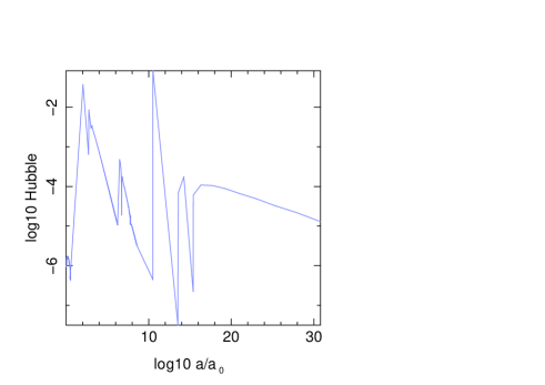
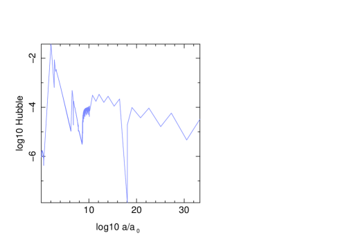
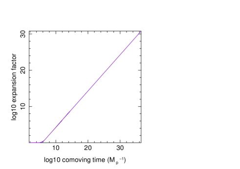
Figure 4: a) and b): Evolution of Hubble function with expansion factor $a(t)$. They are obtained from series of 5 separate successive simulations with different rules for time incrementation to reduce accumulation of numerical errors. Rapid variations may be in some extend numerical artefacts. The difference between plots a) and b) is the initial $a(t)/a_{0}$ in one of the simulations at intermediate $\log_{10}a(t)/a_{0}\sim 8.5$, see the text for details. c) Evolution of expansion factor with time for simulations shown in a).

The initial increase and oscillation of $H$ is due to the rapid evolution of energy-momentum density from being dominated by cold $X$ particles to a binding energy dominated plasma through non-equilibrium interaction between the three constituents of the model. Large oscillations in the Hubble function before the onset of inflation are mainly due to the chaotic behaviour of nonlinear evolution equations. Indeed, approximate analytical solution of evolution equations of the model in [35] shows the presence of a parametric resonance, see following sections for discussion of processes causing such behaviour. Indeed what is happening here is analogous to preheating and exponential particle production at the end of inflation [10]. Moreover, because in these simulations the metric is evolved consistently, the effect of particle production and interaction between various components induces instabilities in the expansion rate and the Hubble function, which backreact on the evolution of densities and may stimulate further instabilities.

4.2.2 Artefact issue

Numerical simulations in general include glitches and artefacts and we cannot rule out that some of the features in our results are artefacts induced by approximations used to simplify computations and by low resolution of these simulations.

To qualify numerical uncertainties we truncated simulations shown in Fig. 4-a at $\log(a/a_{0})\sim 8.5$ and continued with slightly different time steps. Fig. 4-b shows the Hubble function obtained from this second series of simulations. Although details of plots and numerical values of physical quantities in this series of simulations are somehow different from the first one, their overall behaviour is very similar. For instance, in the case of $H(a)$ in Fig. 4-b, despite oscillations at late stages of the simulation, the average slope, i.e. the average $d\log H/d\log a\equiv-\epsilon_{1}$ [89] is similar to that of smooth evolution of the first simulation series shown in Fig. 4-a. Therefore, in the following sections we only discuss the results of the first series of simulations and restrict our conclusions to overall aspects rather than details, which may not be reliable.

Better simulations are necessary for verifying to which extend results and conclusions of these simulations are correct. Comparison with more or less similar simulations is another way of cross-checking the results. For instance, large oscillations of energy-momentum tensor and expansion rate before the onset of inflation are reported by other authors [22] and compared to the instability of QED vacuum. Therefore, despite inevitable numerical effects, initial oscillations in these simulations seem real, and as explained above, a consequence of dynamical instabilities.

4.2.3 Inflation parameters

For determining characteristics of the inflationary epoch in this model - defined as when the Hubble function varies slowly with increasing expansion factor - we fit $\log H(a)$ using parameters $\epsilon_{i},~{}i=1,2$ defined in [89]. We obtain $\epsilon_{1}\sim 0.01-0.04$ and $\epsilon_{2}\sim-0.14~{}-~{}0.35$, depending on the choice of time steps used for the fitting. In classical treatment of inflation models $\epsilon_{i}$ parameters can be analytically related to the spectral index of scalar fluctuations $n_{s}-1=-\epsilon_{2}-4\epsilon_{1}$ and tensor to scalar ratio $r=16\epsilon_{1}$. Comparison of values obtained for $\epsilon$ parameters from our simulations and corresponding values for $n_{s}$ and $r$ shows that according to these relations the model is not consistent with the CMB observations [8]. Even when the value of $n_{s}$ is consistent with observations, $r$ is too large. However, in Sec. 4.2.8 we show that the value of both these parameters obtained directly from simulations are indeed consistent with observations. Therefore, the relation between $\epsilon$’s and properties of the spectrum of fluctuations obtained from classically treated scalar field models cannot be applied to fully quantum non-local approach. We should also remind that the choice of parameters for the simulations were motivated by the results of classical interacting quintessence models studied in [36] and no adjustment was performed to reproduce CMB observations.

4.2.4 Evolution of densities

Effective potential of inflation is a very important quantity because apriori it can be extracted from angular spectrum of CMB and LSS fluctuations [90]. As for the time being cosmological observations are the only accessible conveyor of the physics of early Universe and high energy scales, it is crucial to understand the relation between effective classical quantities extracted from cosmological data and the underlying fundamental model. Observations of the Planck satellite shows no significant non-Gaussianity and is consistent with a small tensor to scalar ratio of $r\lesssim 0.05$. These results indicates a flat effective potential and a small field inflation [8].

Fig. 5 shows the evolution of the 1PI terms in the density $\rho$, that is the second bracket in (2.50), for the three constituents of the model, which from now on we call them $\rho^{i}_{1PI},~{}i=X,A,\Phi$.

a)	b)	c)

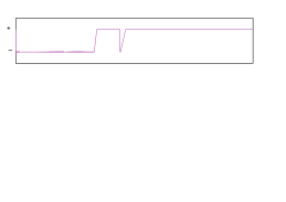
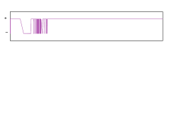
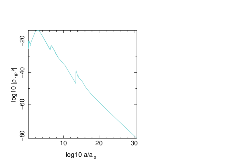
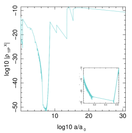
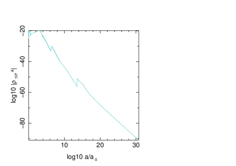
Figure 5: a), b), c): Contribution of 1PI terms $\rho^{i}_{1PI},~{}i=X,A,\Phi$ in the total energy density. The upper plots show the sign of these terms and lower plots their amplitude. The inset in b) is a zoom on the early evolution of $\rho^{X}_{1PI}$.

It is easy to verify that the initial rapid decay of $\rho^{X}_{1PI}$ is not due to what we may call semi-classical decay, i.e. the lowest order tree diagram of $X$ particles decay into $A$ and $\Phi$. With the value of $\mathcal{G}$ chosen for these simulations the decay width of $X$ through this channel is comparable to the present value of Hubble constant, and consequently the lifetime of free $X$ particles is comparable to the present age of the Universe. Our tests show that the slope of this decay depends on the self-coupling $\lambda$ of $\Phi$ and is induced by the sudden increase in the number of these particles and their interaction with $X$, see plots in Fig. 6 which show the evolution of classical potential of the condensate $\varphi$, its effective energy density, and contribution of 2PI terms in the total energy density.

We argue that the large mass difference between $X$ and $\Phi$ and self-interaction of the latter is enough to quickly initiate a cascade production of $\Phi$ particles. In turn, their interaction with energetically dominant but numerically rare $X$ particles transfers their energy to a non-equilibrium quantum binding energy corresponding to 2PI terms in energy-momentum tensor (2.46) or equivalently (2.50). Therefore, despite small couplings the state of matter during this era is non-perturbative and comparable with a strongly coupled plasma, which its instabilities lead to large oscillations - parametric resonance - of densities and Hubble function. The large effective masses of $\Phi$ and its condensate shown in Fig. 7-a are manifestation of their effectively strong interaction during this non-perturbative regime.

It is useful to compare these results with an $O(N)$ model studied in strong coupling regime and Minkowski spacetime [91]. It finds that in the non-perturbative regime, after initial parametric resonance, low momentum modes dominates and the system exhibits an effective weak coupling. Despite apparent contradiction, this finding is consistent with the above results, because due to the limited resolution of these simulations, initially they are concentrated on high momentum modes and parametric resonance of these modes [35] manifests itself in large oscillation of average density and Hubble function. However, with the expansion of the Universe, momentums are redshifted to the domain where coupling between fields are effectively weak and densities and Hubble function behave smoothly, as predicted by [91].

a)	b)	c)	d)

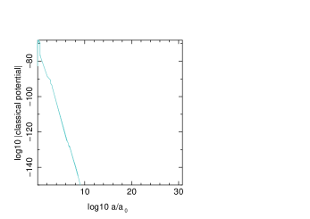
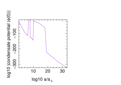
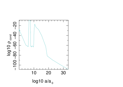
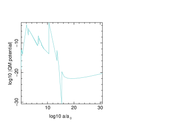
Figure 6: a): Classical potential of condensate $\varphi$; b) Effective potential of condensate, including quantum corrections; c) Effective energy density of condensate; d) Contribution of 2PI terms in the total energy density.

The strong effective coupling of fields does not last for long because at the same time the effective mass of $\Phi$ increases, see Fig. 7-a, and its backreaction decreases the rate of decay of $\rho^{X}_{1PI}$, see the inset in Fig. 5-b and the amplitude of condensate field $\varphi$ in Fig. 6-a. A slow decay rate of $\rho^{X}_{1PI}$ continues for some time before the latter and the density of $\varphi$ increase again, see Fig. 6-b. Repetition of the same processes leads to oscillation of the total density $\rho_{tot}$ reflected in the oscillation of the Hubble function. However, due to the expansion of the Universe, gradually the amplitude of quantum binding energy, shown in Figs. 6-c and its contribution to the total energy density, shown in Fig. 7-b, decreases and a slow evolution of total density leads to a power-law inflation. It is driven by the transfer of quantum binding energy to $X$ field, shown in Fig. 7-c.

a)	b)	c)

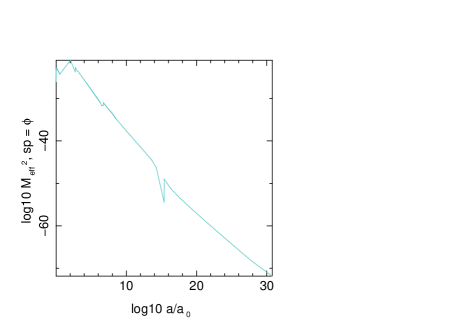
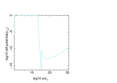
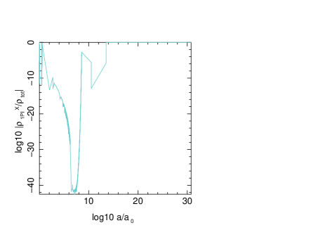
Figure 7: a): Effective $M^{2}_{\Phi}(x=0)$; b) Fraction of zero mode, i.e homogeneous component of effective quantum binding energy density to total average density; c) Ratio of average $\rho^{X}_{1PI}$ to total density.

As expected, the effective masses of $\Phi$ and its condensate $\varphi$ initially include a significant contribution from self-interaction and coupling with heavy field $X$. However, this effect is restricted to high energy modes, see the description of the spectrum of fluctuations in the next Sec. 4.2.8. We remind that accelerating expansion reduces the physical size of simulated modes $k/a(t)$ and the effect of local quantum corrections diminishes. Consequently, the effective mass of quantum fluctuations of $\Phi$ and its condensate $\varphi$ approaches its renormalized value at IR scale and $\varphi\rightarrow 0$. This may be an evidence that a shift symmetry for neutralizing the effect of quantum corrections on the mass of light field $\Phi$ would not be necessary, because rapid expansion automatically suppresses the effect of quantum corrections. This observation also shows the shortcomings of numerical simulations of cosmological models, which are unable - without increasing resolutions - to follow the evolution of growing distance scales with the same precision.

Apriori the effective mass of quantum and condensate components of $\Phi$ are not equal, see diagrams in Figs. 2 and 3. However, in this series of simulations their difference is much smaller than numerical precision and Fig. 7-a presents the mass of both components. We should also remind that $A$ and $X$ fields have no self-interaction, and thereby no local quantum correction to their mass.

4.2.5 Evolution of pseudo-free particles

The behaviour of 1PI contributions of $A$ and $\Phi$ are very different from that of $X$, see Fig. 5. Their densities $\rho^{A}_{1PI}$ and $\rho^{\Phi}_{1PI}$ vary much slower than $\rho^{X}_{1PI}$, which its variation with both time and expansion factor is very sharp and steep, and reminiscent to multiple first order phase transitions. In comparison, the densities of lighter fields behave similar to a slow and continuous second order phase transitions. Moreover, their variation is asynchronous with respect to $\rho^{X}_{1PI}$. The reason behind these differences is not only the large difference in their mass, but also their interactions. Notably, due to its self-interaction $\Phi$ field which has the smallest mass, attains much higher densities than $A$. The systematically asynchronous onset of features and sign changes for different fields and components are the evidence that despite low quality of these simulation complex behaviour of fields and their properties must be grossly genuine and cannot be completely numerical effects. These features coarsely demonstrate the fully non-equilibrium nature of underlying processes. However, as we discussed at the beginning of this section and demonstrated with Figs. 4-a and 4-b, we do not rely on the details in our conclusions.

a)	b)	c)

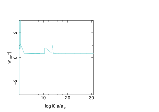
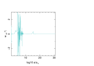
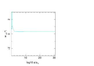
Figure 8: a), b), c): Equation of state for 1PI components of the energy-momentum tensor of $\Phi$, $X$ and $A$, respectively.

Another interesting characteristic of 1PI contributions of the fields is the negative sign of $\rho^{i}_{1PI},~{}i=X,A,\Phi$ in some era. This means that these components of total density cannot be considered as belonging to truly free particles. Nonetheless, after initial instabilities, their equation of state defined as: $w^{i}_{1PI}\equiv p^{i}_{1PI}/\rho^{i}_{1PI}$, approaches to zero for $X$ and to $1/3$ for $A$ and $\Phi$, see Fig. 8. Thus, they behave similar to non-relativistic and relativistic free particles, respectively. This observation justifies the interpretation of $\rho^{i}_{1PI},~{}i=\Phi,X,A$ as pseudo-free particles and shows that the process of inflation and particle production are inseparable. Because in this toy model $X$ is much heavier than other fields and its lifetime as free particles is very long, at the last stages of inflation it dominates as a cold matter. However, it is conceivable that if its life time is shorter, at the end of inflation light fields become dominant and induce a radiation domination era, as expected in a hot Big Bang model. We did not study such a case.

4.2.6 Effective potential and condensate

Total density $\rho$ and specific enthalpy, defined as $\rho+p$, are shown in Fig. 9. They are both positive (up to numerical errors for the latter) and there is no violation of null energy principle in the simulations.

Comparison of condensate density shown in Fig. 6-b with the total density and other components of energy-momentum demonstrates that its contribution is completely negligible. Moreover, the comparison of Figs. 6-b and 6-c shows that after the onset of inflation, assumed to be at $log(a/a_{0})\gtrsim 15$, the energy density of condensate $\rho_{\varphi}$ is dominated by its kinetic energy (not shown here) rather than its effective potential. These observations are consistent with approximate analytical results reported in [35], which show that the condensate can grow during radiation domination era, when expanding is relatively slow. But it decays during matter domination and by extension during inflation eras, which have faster expansion rate.

Figs. 7-b and 7-c show that in these simulations inflation is supported by the decay of quantum binding energy to particles. They also indicate that during inflation a significant fraction of quantum binding energy goes to the formation of $X$ particles. However, this may be in part due to the stiffness of the model and imprecision of simulations, which capture more easily the heavy $X$ particles rather than lighter fields. Nonetheless, as mentioned earlier, this observation is consistent with some analytical calculations for simpler models [22]. Moreover, early works and some recent studies of the evolution of scalar quantum fields in an expanding universe show particle production processes and their impact on the expansion [93]. Therefore, our results may be a confirmation of previous studies. In any case, this aspect of the model needs confirmations by better simulation. on the other hand, in contrast to some studies [94], the initial large oscillations of densities do not leave observable oscillations in the dominant matter component $X$ - presumably dark matter - at late times. Further arguments in favour of claim will be given in Sec. 4.2.8.

a)	b)

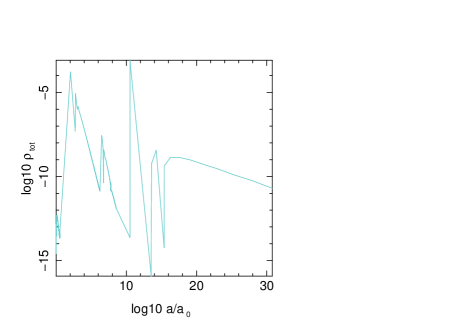
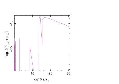
Figure 9: a): Total energy density; b) Total specific enthalpy $\rho+P$. Upper plots: sign; Lower plots: amplitude.

The above results and observations indicate that the relation between properties of inflation parameters $\epsilon_{i}$, extracted from observations, and characteristics of the underlying model, e.g. self-interaction of inflaton field, is not straightforward. For instance, although the light field $\Phi$ and its condensation have very important role in the control of quantum processes which lead to inflation, its contribution in the classical effective energy-momentum density may be insignificant. Moreover, in contrast to single field monomial models, the energy density of condensate $\varphi$ during inflation may be dominated by its kinetic energy rather than its potential. However, this property would be undetectable from $\epsilon_{i}$. In slow-roll monomial models of inflation by definition the potential energy must dominate the energy density. However, as the inflation in the model studied here is conducted by other components, this is not a necessary condition for making the model consistent with observations. Nonetheless, the dominance of kinetic energy of the condensate has an impact on the spectrum of fluctuations of the condensate, which we will discuss in Sec. 4.2.8.

4.2.7 Stronger self-coupling

For the sake of comparison Fig. 10 shows the evolution of Hubble function, effective mass of $\Phi$, ratio of quantum 2PI binding energy to total energy density, and properties of the condensate $\varphi$ for a model with $\lambda=10^{-8}$ and other parameters the same as the simulations discussed above. In this case the estimation of initial rate of condensate formation (3.35) gives $\Gamma_{\varphi}/H\gg 1$ at initial time. Therefore, it is expected that condensate has a more significant contribution in the total energy density of the Universe. Indeed, we observe significant differences between properties of condensate in this model and simulations with $\lambda=10^{-14}$. Notably, the heavy particle production and inflation begin much earlier. This is due to the higher effective mass of $\Phi$ particles at a given epoch, that is a fix $a$, see Fig. 10-b. However, although the larger coupling constant increases classical potential energy, it remains much smaller than quantum binding energy and kinetic energy of the condensate shown in Fig. 10-e. On the other hand, the effective energy density of condensate, shown in Fig. 10-f, is dominated by quantum corrections during inflation, and consequently its equation of state $w_{\varphi}\sim-1$. Nonetheless, during inflation $\rho_{\varphi}$ is not constant and decreases as $\sim a^{-2}$. Apparently, this violates the usual relation between $w$ and evolution of density with expansion factor. However, the density of condensate alone is not conserved and its interaction with other components of the model must be taken into account. If the condensate continues the same trend after inflation, it cannot be a candidate for dark energy. However, at the end of inflation if its decline slows down and its density asymptotically approaches to a constant density, as analytical approximations has shown [35], the small leftover may explain the observed accelerating expansion of the Universe at present era. Unfortunately, for the time being simulations cannot be extended to these late epochs with enough precision to capture these details.

These observations raise the issue of the end of inflation. In the present simulations we do not observe an end to inflation. However, based on earlier behaviour of model we expect that a change in the contribution of different components of energy-momentum induces again a phase transition. An evidence for such behaviour is the gradual increase of quantum binding energy at the end of simulations in Figs. 6-d and 10-c. However, we cannot be sure that this is not an artefact, specially because it includes only a few time steps in our simulations.

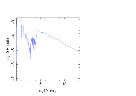
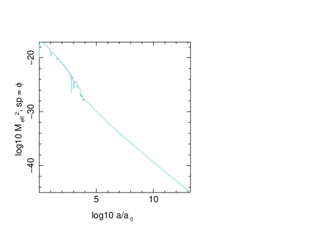
a)	b)	c)
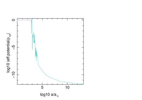
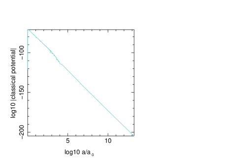
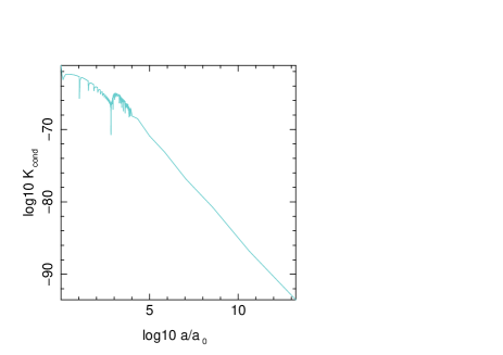
d)	e)	f)

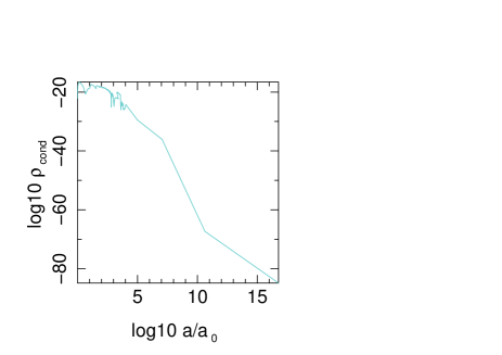
Figure 10: Properties of the model with $\lambda=10^{-8}$. a) Hubble function; b) Effective mass $M^{2}_{\Phi}$  c) Ratio of quantum binding energy to total energy density; d) Classical potential of condensate $\varphi$; e) Effective potential of condensate; f) Effective energy density of condensate $\varphi$;

4.2.8 Spectrum of fluctuations

Although horizon flow and its derivatives $\epsilon_{i},~{}i=0,1,2,3,\cdot$ are usually used for parametrizing inflation models, only for the simplest among them, in particular a single scalar field in slow-roll regime, they can be considered as reliable proxies for spectrum of primordial fluctuations. Therefore, for a stiff multi-field model in a non-equilibrium state, as the one discussed here, it is better to investigate the spectrum of fluctuations directly.

Fig. 11 shows the evolution of normalized exact propagators $G^{F}_{i}(k,t)/G^{F}_{i}(k=0,t),~{}i=\Phi,X,A$ during inflation era, calculated numerically up to second perturbative order and under approximations discussed at the beginning of this section. We remind that for free fields $G^{F}_{i}(k,t)\equiv 2N_{k}+1$ where $N_{k}$ is proportional the expectation value of particle number in mode $k$. For interacting fields $N_{k}$ can be considered as an effective number. Fig. 12 shows the spectrum of fluctuations of various components of $T^{00}$, which for a homogeneous background metric corresponds to energy density.

a)	b)
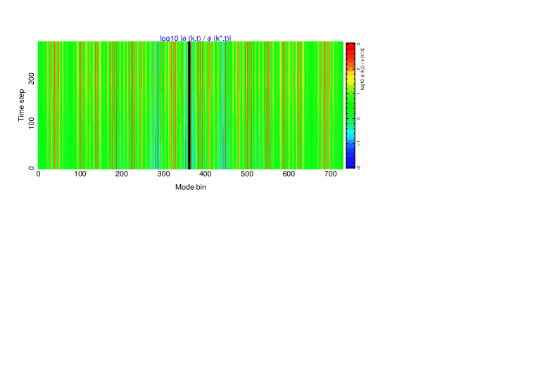
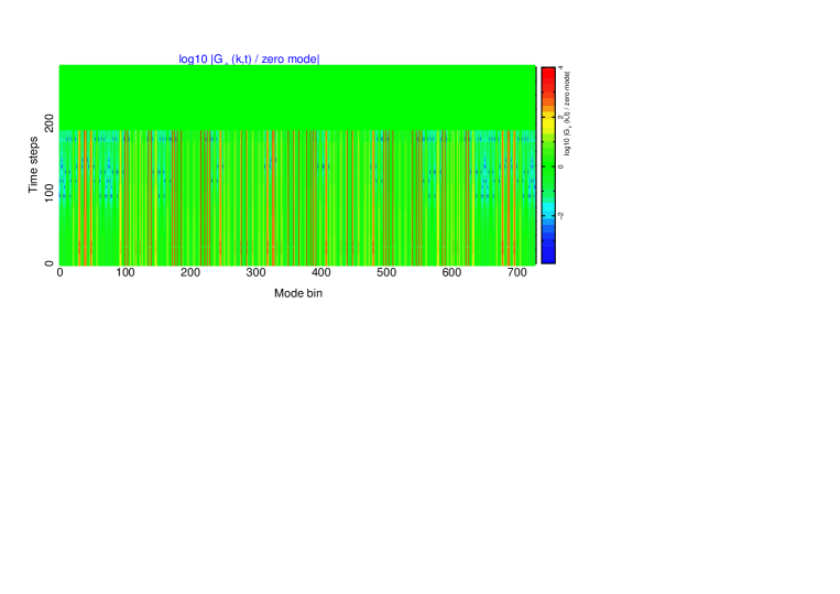
c)	d)

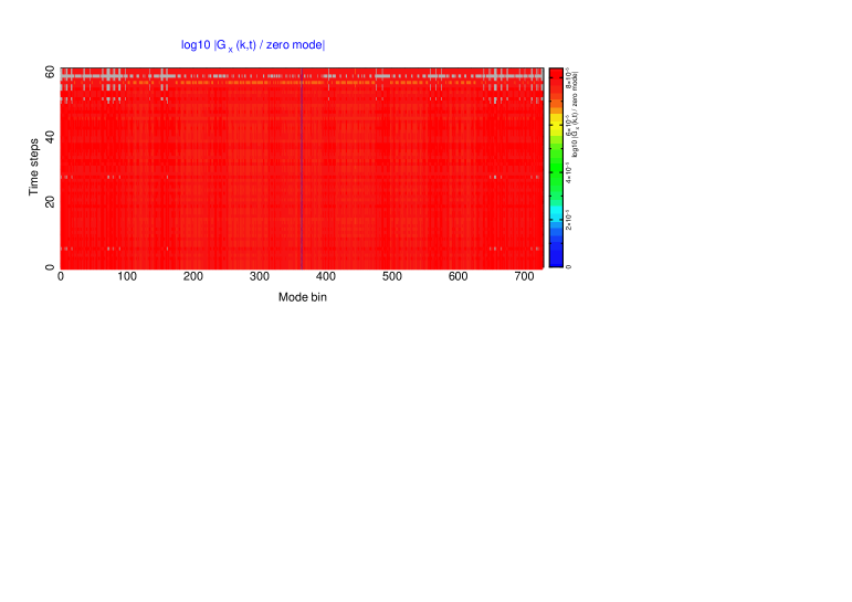
Figure 11: a) Color coded normalized spectrum of condensate $\varphi(k,t)/\varphi(k^{*},t)$ where $k*$ has the largest amplitude in the simulation box. b), c) and d) Color coded normalized exact propagators $G^{F}_{i}(k,t)/G^{F}_{i}(k=0,t),~{}i=\Phi,~{}X,~{}A$, respectively. The x-axis presents a cube of $9^{3}$ channels in the mode space. They are arranged such that $|k|=0$ corresponds to channel $364$. An example of the 3D modes is shown in Fig. 12-f. The value of $k$ in this plot is with respect to conformal coordinate and does not depend on time. The corresponding physical (comoving) mode is $k/a$. The y-axis presents simulation time steps as explained in footnote 25. To better highlight variation in amplitude of modes in a) and b) all the registered time intervals are used, but c) and d) show only data during inflation. The apparently abrupt change in the spectrum of $G^{F}_{\Phi}(k,t)/G^{F}_{\Phi}(k=0,t)$ is partly because of adaptive time steps which varies in different stages of simulation, and partly due to the absence of some intervals from plots, as explained in footnote 25.

a)	b)
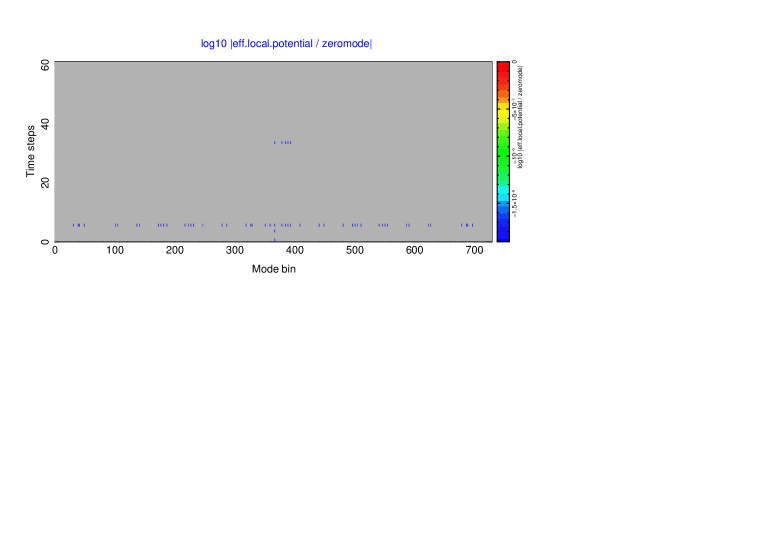
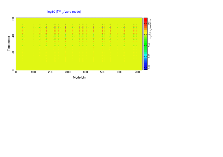
c)	d)
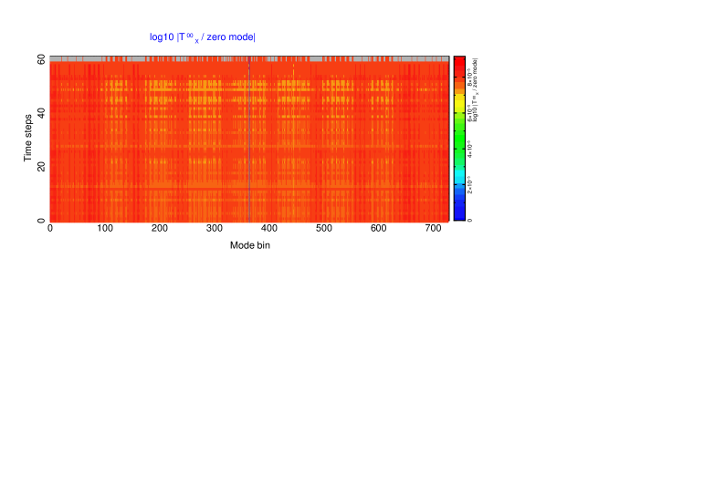
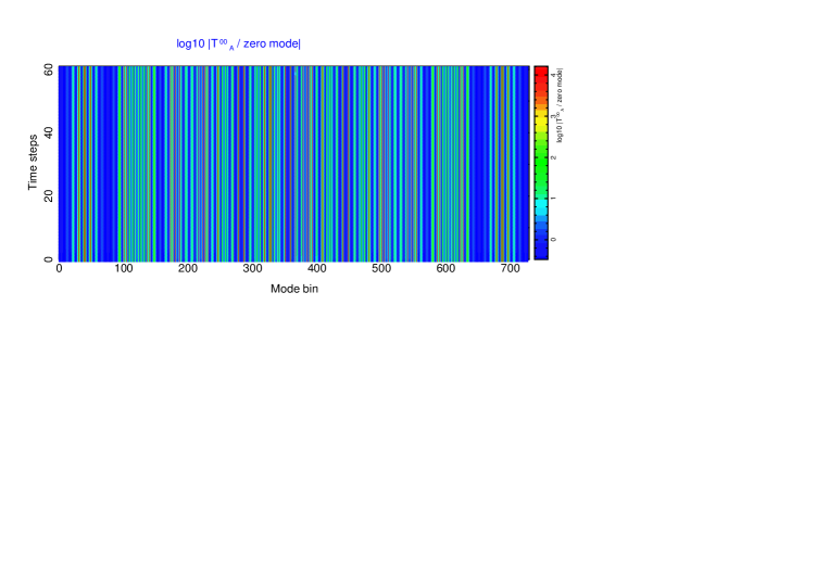
e)	f)

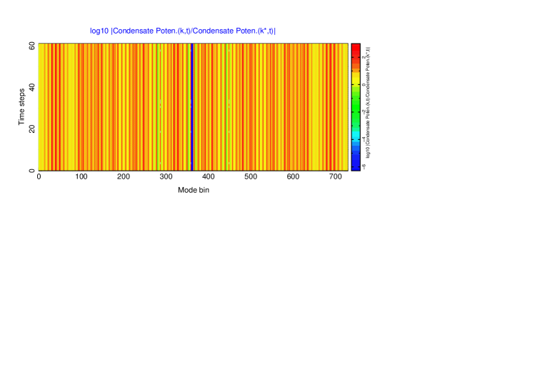
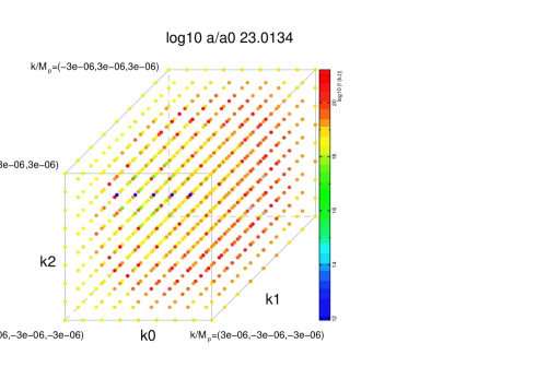
Figure 12: Spectrum of energy density components: a) 2PI quantum binding energy density normalized to its zero mode. Color gray corresponds to upper limit, which in this plot is zero and corresponds to an scale invariant amplitude; b), c), d) $T^{i}_{1PI}(k,t)/T^{i}_{1PI}(k=0,t),~{}i=\Phi,~{}X,~{}A$, respectively; e) energy density of condensate normalized to its zero mode. Description of axis is the same as in Fig. 11; f) Color coded amplitude of $a\varphi$ modes in the mode cube during one simulation time step. Values of modes are in $M_{p}$ unit.

As we discussed in Sec. 4.2.5, at late stages of inflation the density of the Universe is dominated by $X$ particles, or more precisely the 1PI component of energy-momentum tensor. The first conclusion from these plots is that the amplitude of fluctuations in this model is ${\mathcal{O}}(1)\times 10^{-5}$, thus consistent with observations. Moreover, the evolution of fluctuations is very close to adiabatic, defined as $\delta N_{k}(a(t))/N_{0}(a(t))=const.$, see e.g. [92] for review. The amount of variation with time of this quantity, assumed as presenting isocurvature fluctuations, is $\lesssim 10\%$. Considering low resolution of our simulations, this value is roughly consistent with the Planck constraint on the fraction of isocurvature perturbation of a few percents [8].

Fluctuations of 2PI quantum corrections are very small even at early stages of inflation. This reflects the non-local nature of this component, which couple different scales together and wash out their differences, even when they are superhorizon. 1PI fluctuations of $X$, which is the dominant component at the end of our simulations, is of order $\mathcal{O}(1)\times 10^{-5}$ and comfortably consistent with observations. However, we observe significant fluctuations in the energy density of condensate $\varphi$ and in 1PI contributions of $\Phi$ and $A$ fields. 1PI components of $\Phi$ and $A$ include tree Feynman diagrams with $X$ as interaction field. Considering the large mass of $X$ particles, these diagrams can be approximated by local interactions. For this reason the fast expansion of the Universe during inflation suppresses interaction at superhorizon scales and only induces oscillations at shorter scales. This process is analogous to Doppler peaks in the present power spectrum, generated by interaction of photons with baryons and free streaming. However, in contrast to baryons, the contribution of $\Phi$ and $A$ in the total energy density and their fluctuations are highly subdominant and would not be observable. On the other hand, as we discussed in Sec. 4.2.6 the dominance of $X$ at the end of these simulations may be due to the stiffness of the model. Moreover, a larger coupling $\mathsf{g}$ decreases the lifetime of $X$ particles and thereby their final density. Then, the self-interaction of $\Phi$ and its interaction with $A$ exchanging virtual heavy $X$ particles should uniformize their fluctuations during a regime analogous to reheating. On the other hand, if large fluctuations survive reheating, they may have some effect at small distant scales as seeds and contribute in the formation of galaxies and/or supermassive black holes.

a)	b)	c)

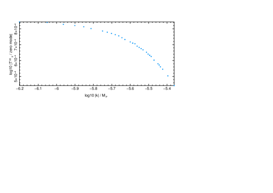
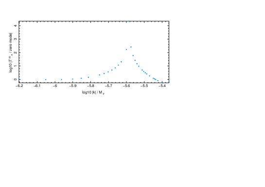
Figure 13: Spectrum of 1PI components at the end of simulations with $\lambda=10^{-8}$. Deviation from a line in a) is due to numerical effects, which have slightly violated isotropy in 3D mode space.

The properties of the power spectrum is better discernible in 1D plots. Fig. 13 shows 1D power spectrum of $T^{i}_{1PI}(k,t)/T^{i}_{1PI}(k=0,t),~{}i=\Phi,~{}X,~{}A$ at the end of simulations for the case of $\lambda=10^{-8}$. It is evident that they are not a power law. Nonetheless, the spectrum of $T^{X}_{1PI}$ which is the dominant component of energy momentum tensor at late times is self-similar and close to a power-law with $n_{s}-1\lesssim 0$. Thus, it is consistent with CMB observations. We emphasize that we have not adjusted parameters of the simulations to reproduce observed cosmological quantities and the purpose of comparison with observations is to see whether their general characteristics are close to observations. For instance, simulations with $\lambda=10^{-14}$ leads to $n_{s}-1\approx 0$ or very slightly positive.

a)	b)	c)

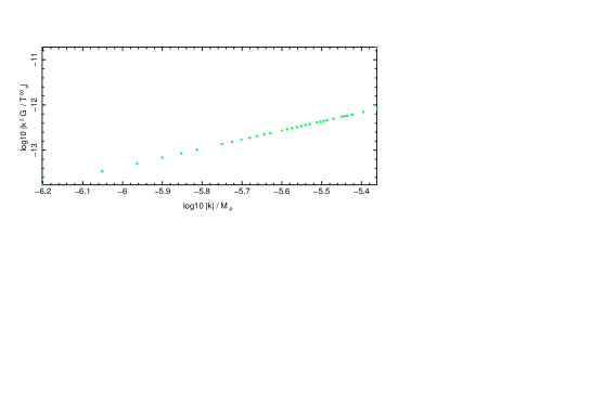
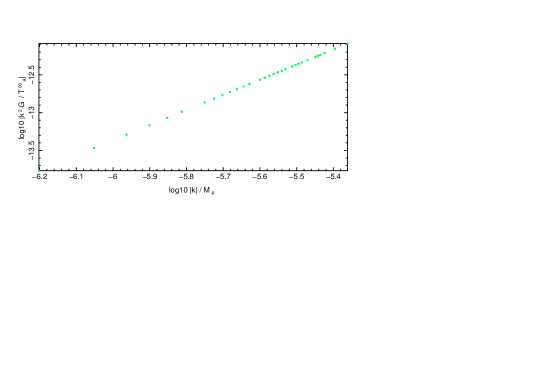
Figure 14: Ratio of anisotropic shear to scalar fluctuations for the fields of the model as an order of magnitude estimation of tensor to scalar ratio $r$.

Although our simulations use a homogeneous metric and cannot determine tensor modes, here we try to find an order of magnitude estimation for tensor to scalar ratio $r$. In the effective fluid description of energy-momentum tensor the anisotropic shear (2.52) generates tensor fluctuations $h_{ij}$ in the metric (2.53). If we calculate the shear generated in a homogeneous background metric, it is straightforward to see that $\Pi^{\mu\nu}(k,t)\propto k^{i}k^{j}G(k,t)$. Therefore, the amplitude of gravitational waves (without taking into account their backreaction) is $\sim k^{2}G(k,t)$. Fig. 14 shows $k^{2}G/T_{1PI}$ as a function of $k$ at the end of simulations for the three fields of the model. The ratios are very small for all the fields. This result is expected because none of components of the energy-momentum tensor in this model becomes at any moment (trans)Planckian. A more precise estimation of $r$ needs simulations which include evolution of metric fluctuations.

4.3 Dark energy

As we described in the Introduction, the model studied here was first suggested and investigated as a candidate explanation for dark energy. The purpose of the present work was to extend earlier studies to a full non-equilibrium quantum field theoretical formulation. According to this model dark energy is the condensate of the light scalar field $\Phi$. The condensate might have been produced during inflation and evolved in such a way that its present effective equation of state $w_{\varphi}\sim-1$ and its density approximately constant. In this case, it can be considered as the remnant of inflation. Alternatively, dark energy condensate may be associated to the decay of a heavy particle - presumably dark matter or a constituent of it - produced after inflation.

Simulations presenting inflation and evolution of various components of the model in the previous subsection showed that the fast expansion of the Universe during this epoch significantly suppresses the condensate. Consequently, its remnant may become too diluted with the expansion of the Universe to be consistent with the observed density and equation of state of dark energy. To see whether the second option, that is the decay of a heavy particle after inflation, can produce a dark energy condensate, we simulated the same model with an initial value of Hubble function expected for the epoch after reheating of the Universe, namely $H_{0}=10^{-15}-10^{-13}~{}M_{P}\sim 10^{4}-10^{6}$ GeV. In addition to the same parameters as the case of inflation, we also performed simulations with $\lambda=10^{-17},~{}\mathsf{g}/M_{P}=10^{-20}$ and $m_{X}=10^{-8}M_{P}$. The reason for reducing the mass of main matter source is lower energy scale of physical processes after preheating. Due to limited numerical resolution of simulations, we were also obliged to reduce its coupling to other fields, otherwise we had to reduce time steps, which made simulations too long. Unfortunately, even in this modified model we were only able to have a crud simulation of late time evolution. Here we present the results of these simulations and describe features that we judge reliable. However, better simulations are necessary to confirm them.

We call simulations with $\mathsf{g}/M_{P}=10^{-17}$ and $m_{X}=10^{-3}M_{P}$ Model 1 and simulations with $\mathsf{g}/M_{P}=10^{-20}$ and $m_{X}=10^{-8}M_{P}$ Model 2. Up to precision of our simulations Model 1 behaves very similar to inflation described in the previous section. For this reason we do not explain it in detail. Nonetheless, it demonstrates that the model described here behaves in a self-similar manner and a shift of initial time, or equivalently initial Hubble constant, simply shift in time the accumulation of quantum binding energy, which ultimately leads to inflation. Thus, the model is not fine-tuned.

Fig. 15-a shows the evolution of $w_{eff}\equiv\rho/p$ in Model 2, where $\rho$ and $p$ are defined in (2.48). As expected, it evolves from matter domination, that is $w_{eff}=0$ to $w_{tot}\approx-1$. We notice that the beginning of transition from matter domination is much earlier than what is observed in cosmological data. However, this regime of the simulations includes only a few time steps and some deviation from real cosmologies in a toy model is expected. We remind that the heating of the Universe occurs in the SM sector, which is not present in our simplistic model of early Universe.

Figs. 15-b and 15-c show the effective $M^{2}_{\Phi}$ and $M^{2}_{\varphi}$. Similar to the case of inflation, after the initial increase of the effective mass due to accumulation and condensation of $\Phi$ field, its value sharply decreases and approaches its IR limit during the phase transition from matter domination to an accelerating expansion. We notice a difference between the effective mass of $\Phi$ and $\varphi$ such that $M^{2}_{\Phi}>M^{2}_{\varphi}$ at any time. As discussed earlier, this is due to the difference in Feynman diagrams which contribute to these effective masses. The comment about too early onset of phase transition discussed for Fig. 15-a applies here too.

a)	b)	c)

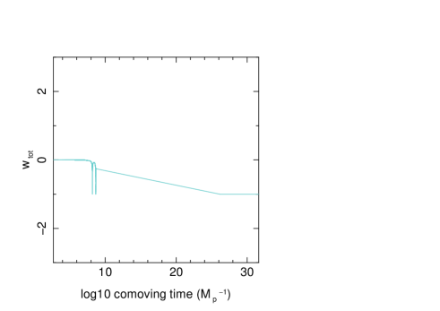
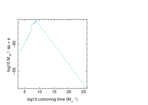
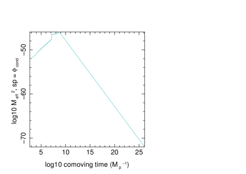
Figure 15: Evolution of effective quantities with time in Model 2 simulating late accelerating expansion of the Universe: a) Evolution of total equation of state; b) Evolution of effective mass of $\Phi$ field; c) Evolution of effective mass of condensate.

Figs. 16-a, 16-b, and 16-c show classical potential of the condensate, quantum binding energy, and its fractional contribution to the total energy density in Model 2, respectively. Similar to the case of inflation, the contribution of classical potential is completely negligible and even the addition of quantum corrections in the effective potential (not shown here) does not make the contribution of condensate in the total energy density significant. However, the sharp increase in quantum corrections is certainly due to the low resolution of our simulations. Most of other conclusions which we discussed for inflation apply also to the late accelerating expansion and do not need to be repeated.

a)	b)	c)

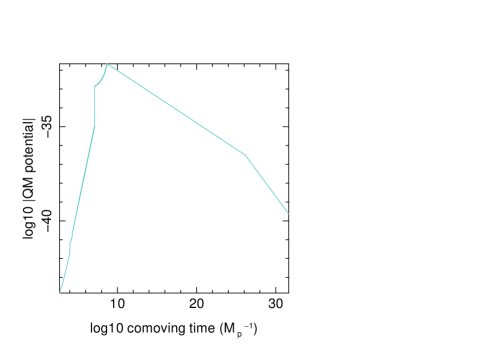
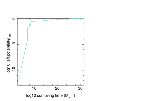
Figure 16: Evolution of classical and quantum components of effective energy density with time in Model 2: a) Classical potential of condensate; b) Effective quantum potential; c) Ratio of effective quantum potential to total energy density.

5 Discussion

We do not see an excess in longest modes, neither in inflation nor dark energy simulations. Therefore, there is no evidence of IR instability in this model. Up to precision of our simulations this result confirms the approximate analytical results obtained for de Sitter space in [25, 26, 28]. Our simulations show that, as expected, the light field acquires an effective time dependent mass. Moreover, after dissipation of initial instabilities, the hierarchy of masses is recovered and when inflation approaches to its end and when dark energy become dominant, the mass $\Phi$ and its condensate approaches their initial values. We should however remind that in our simulations this field is not massless. Therefore, the above conclusion is not in contradiction with [18], which finds IR instability only for massless fields.

In its simplest form considered here the model does not have internal symmetry, but it can be easily extended to such cases. Our simulations show that at initial stages of inflation a condensate form, and therefore internal symmetries break. However, the amplitude of the condensate would be very small, specially during inflation and late accelerating expansion. This means that there may be Goldstone boson due to symmetry breaking, but it would not be completely massless. This may explain the small but nonzero mass of $\Phi$.

The fast decay of condensate component during accelerating expansion is consistent with the results of [35]. However, the small contribution of condensate in the total energy density even before fast acceleration found here is in contradiction with conclusions of [35], which predicts that a significant amount of condensate may survive the expansion. One of the reasons for this difference may be the lack of consistent evolution of expansion factor in approximative analytical method employed in [35]. Moreover, the latter analysis is mostly concentrated on finding time variation of condensate rather than comparing its contribution in the total density. In any case, both analytical approach in [35] and numerical simulations here are far from perfection and better analytical techniques and/or simulations are necessary to confirm or refute these findings.

Results of our simulations raise an important question: How can we discriminate between a quantum binding energy and an effective classical potential in cosmological observations ? Even for cases in which experiments can be performed in laboratory discrimination between quantum and classical correlations is not easy. For instance, although measurement of the spectrum of excited electrons in atoms can be relatively easily achieved, performing similar experiments for strongly coupled partons in hadrons or weakly coupled molecules is very difficult. In the former case the strong coupling makes isolation of one parton extremely difficult, and in the latter example thermal noise and strong interaction of a probe with atoms intertwine and influence the measurement of a weak molecular binding energy. In cosmological measurements correlation between causally decoupled modes may help to discriminate non-local quantum effects. But, due to the expansion of the Universe it is not trivial to discriminate between correlations induced by past causal interactions and inherently non-local quantum effects. The observation of non-Gaussianity may be a signature, but as we saw in the simulation of inflation, the amplitude of fluctuations of the quantum component, and thereby its non-Gaussianity, is very small.

A point which is not addressed in this work is the effect of unobservable IR modes. They are suggested to be responsible for the late accelerating expansion [96], but so far the issue is not investigated in a fully quantum setting. In the framework of 2PI formulation the incompleteness (openness) of cosmological observations is presented by a mixed density matrix, which is not considered here. Nonetheless, analysis for a toy model in de Sitter space at lowest quantum order [97] shows that IR modes dissipate. This is consistent with our simulations of pure states. Another issue that low resolution of our simulations did not allow to investigate is a relation between inflation and dark energy. We showed that most probably inflaton condensate does not survive inflation and its remnant would be too diluted to generate another epoch of accelerating expansion at later times. However, as we demonstrated, the quantum binding energy of the same fields may induce late time accelerating expansion. We were not able to connect the two epochs. This needs a detail simulation of particle production at the end of inflation, which couldn’t be followed with our code.

There is also a need for exploring more extensively parameter space and extensions to this model, namely: larger coupling among the three fields, self-coupling of other fields, other combination of masses, other coupling models, internal symmetries, gauge symmetry, etc.

6 Outlines

In conclusion, we studied a simple multi-component model for early and late accelerating expansion of the Universe in a fully quantum field theoretical framework. Through numerical simulation we investigated the process of formation of a quantum condensate from an initially null state and followed its evolution, as well as the evolution of quantum component of the fields and their effect on the geometry of the Universe.

We assessed the reliability of simulations by changing resolution and break points of intermediate simulations. We also performed simulations with different masses and couplings. We observed that although small scale features in the evolution curves are not reliable, general behaviour of quantities do not significantly depend on the simulation setup. Interpretations and conclusions discussed in previous sections and summarized below are restricted to general aspects rather than features which may be artefacts. Evidently and as usual better simulations are necessary to confirm our conclusions.

Our simulations show that in realistic models containing multiple fields and hierarchy of masses and couplings, the non-local binding energy between interacting constituents, which depends on all fields, rather than the condensate may have important role in triggering inflation and generation of anisotropies and/or late accelerating expansion of the Universe. On the other hand, although energetically subdominant, numerical domination of light field quanta has crucial role in controlling the behaviour of heavier fields, and thereby the content and geometry of the Universe. This highlights the shortcomings of making conclusions about fundamental physics of early Universe by comparing cosmological data with predictions of classical or semi-classical models of inflation and dark energy. Additionally, it demonstrates that many quantum phenomena, which cannot be described by classical effective models, might have dominated processes leading to the Universe as we find it now.

Appendix A Classical potential

Classical potential in (2.1) and its first and second derivatives are:

$$\mathcal{V}(\Phi,A,X)=\frac{1}{2}m_{\Phi}^{2}{\Phi}^{2}+\frac{\lambda}{4!}{\Phi}^{4}+\frac{1}{2}m_{X}^{2}X^{2}+\frac{1}{2}m_{A}^{2}A^{2}-\mathsf{g}\Phi XA$$ (A.1)

$$\frac{\partial\mathcal{V}}{\partial\Phi}=m_{\Phi}^{2}\Phi+\frac{\lambda}{3!}{\Phi}^{3}-\mathsf{g}XA,\quad\quad\frac{\partial\mathcal{V}}{\partial X}=m_{X}^{2}X-\mathsf{g}\Phi A,\quad\quad\frac{\partial\mathcal{V}}{\partial A}=m_{A}^{2}A-\mathsf{g}\Phi X.$$ (A.2)

$$\frac{\partial^{2}\mathcal{V}}{\partial\Phi^{2}}=m_{\Phi}^{2}+\frac{\lambda}{2!}{\Phi}^{2}\quad\quad\frac{\partial^{2}\mathcal{V}}{\partial X^{2}}=m_{X}^{2}\quad\quad\frac{\partial^{2}\mathcal{V}}{\partial A^{2}}=m_{A}^{2}$$ (A.3)

$$\frac{\partial^{2}\mathcal{V}}{\partial\Phi\partial X}=-\mathsf{g}A\quad\quad\frac{\partial^{2}\mathcal{V}}{\partial\Phi\partial A}=-\mathsf{g}X\quad\quad\frac{\partial^{2}\mathcal{V}}{\partial X\partial A}=-\mathsf{g}\Phi$$ (A.4)

There are 3 extrema points indexed as $0,1,\&2$:

$$\Phi_{0}=A_{0}=X_{0}=0$$ (A.5)

$$X_{1,2}=\pm\biggl{(}\frac{\lambda m_{X}^{2}m_{A}^{4}}{3!\mathsf{g}^{4}}+\frac{m_{\Phi}^{2}m_{A}^{2}}{\mathsf{g}^{2}}\biggr{)}^{\frac{1}{2}},\quad\quad\Phi_{1,2}=\frac{m_{X}m_{A}}{\mathsf{g}},\quad\quad A_{1,2}=\frac{\mathsf{g}\Phi_{1,2}X_{1,2}}{m_{A}^{2}}$$ (A.6)

Second derivative (A.3) and (A.4) show that the trivial minimum (A.5) is the true minima of the system. For both positive and negative $\mathsf{g}$ other extrema are unstable.

For the value of parameters used in the simulations $|X_{1,2}|=10^{-6}/\sqrt{3!},~{}A_{1,2}=10^{-4},~{}\Phi_{1,2}=0.1$. Therefore, even at classical level the amplitude of condensates of $X$ and $A$ at quasi-equilibrium is much smaller than that of $\Phi$ and neglecting them in the simulations is justified.

Appendix B Propagators and decomposition of self-energy

For a bosonic field $\psi$ propagators are defined as (for $\langle\psi\rangle=0$):

$$G^{F}(x,y) \equiv \frac{1}{2}\langle\{\hat{\psi}(x),\hat{\psi}^{\dagger}(y)\}\rangle=\frac{i}{2}(G^{>}+G^{<})$$ (B.1)

$$G^{\rho}(x,y) \equiv i\langle[\hat{\psi}(x),\hat{\psi}^{\dagger}(y)]\rangle=-(G^{>}-G^{<})$$ (B.2)

$$iG^{>}(x,y) \equiv \langle\hat{\psi}(x)\hat{\psi}^{\dagger}(y)\rangle=\text{tr}(\hat{\psi}(x)\hat{\psi}^{\dagger}(y)\hat{\varrho})$$ (B.3)

$$iG^{<}(x,y) \equiv \langle\hat{\psi}^{\dagger}(y)\hat{\psi}(x)\rangle=\text{tr}(\hat{\psi}^{\dagger}(y)\hat{\psi}(x)\hat{\varrho})$$ (B.4)

$$G_{Fey}(x,y) \equiv -i\langle T\hat{\psi}(x)\hat{\psi}^{\dagger}(y)\rangle$$ (B.5)

$$= G^{>}(x,y)\Theta(x^{0}-y^{0})+G^{<}(x,y)\Theta(y^{0}-x^{0})$$

$$= G^{F}(x,y)-\frac{i}{2}\text{sign}(x^{0}-y^{0})G^{\rho}(x,y)$$

$$\bar{G}_{Fey}(x,y) \equiv -i\langle\bar{T}\hat{\psi}(x)\hat{\psi}^{\dagger}(y)\rangle$$ (B.6)

$$= G^{>}(x,y)\Theta(y^{0}-x^{0})+G^{<}(x,y)\Theta(x^{0}-y^{0})$$

$$= G^{F}(x,y)+\frac{i}{2}\text{sign}(x^{0}-y^{0})G^{\rho}(x,y)$$

where $T$ and $\bar{T}$ time ordering and inverse ordering operators, respectively. When $\langle\psi\rangle\neq 0$, $G^{F}(x,y)=G^{F}(x,y)\biggl{|}_{\langle\psi\rangle=0}-~{}\langle\psi(x)\rangle\langle\psi(y)\rangle$.

Properties of propagators can be summarized as the followings:

$$[iG^{>,<}(x,y)]^{\dagger}=iG^{>,<}(y,x),\quad\quad iG^{>}=G^{F}-\frac{i}{2}G^{\rho},\quad\quad iG^{<}=G^{F}+\frac{i}{2}G^{\rho}$$

$$G^{F~{}\dagger}(x,y)=G^{F}(x,y),\quad\quad G^{\rho~{}\dagger}(x,y)=-G^{\rho}(y,x)$$ (B.7)

Here $\hat{\varrho}$ is the density operator of the quantum state of the system. The advantage of using $G^{F}(x,y)$ and $G^{\rho}(x,y)$ is that they include both time paths and their evolution equations are explicitly causal and suitable for numerical simulations [44].

In a similar manner the self-energy $\Pi(x,y)$ can be decomposed to symmetric (F) and anti-symmetric ($\rho$) components [44]. For this purpose we first separate local component of the self-energy, then we decompose non-local part in analogy with (B.5):

$$\Pi(x,y) \equiv -i\Pi^{0}(x)\delta^{(4)}(x-y)+\bar{\Pi}(x,y)$$ (B.8)

$$M^{2}(x) \equiv m^{2}+\Pi^{0}(x)$$ (B.9)

$$\bar{\Pi}(x,y) \equiv \Pi^{F}(x,y)-\frac{i}{2}\text{sign}(x^{0}-y^{0})\Pi^{\rho}(x,y)$$ (B.10)

By using the decomposition of Feynman propagator (B.5) in self-energy diagrams we obtain the following expression for contribution of a diagram including $k$ propagators:

$$\Pi^{F} \propto \sum_{j=0}^{[k/2]}C^{k}_{k-2j}(-1)^{j}2^{-2j}G_{F}^{k-2j}G_{\rho}^{2j}$$ (B.11)

$$\Pi^{\rho} \propto \sum_{j=0}^{[k/2]}C^{k}_{k-2j-1}(-1)^{j}2^{-2j}G_{F}^{k-2j-1}G_{\rho}^{2j+1}$$ (B.12)

where $[k]$ is the integer part of $k$. Here we have used proportionality sign rather than equality because couplings, number of degeneracies, and traces are not shown in (B.11) and (B.12). These factors depend on the topology of corresponding Feynman diagram, order of interactions and 1-point expectation value. They are the same for both components.

Appendix C Density matrix of a many-particle state

A pure quantum many-particle state can be decomposed as:

$$[a_{\beta_{1}},a^{\dagger}_{\beta_{2}}]=\delta_{\beta_{1}\beta_{2}}\quad[a_{\beta_{1}},a_{\beta_{2}}]=0\quad[a^{\dagger}_{\beta_{1}},a^{\dagger}_{\beta_{2}}]=0$$ (C.1)

$$|\Psi\rangle\equiv\sum_{\beta_{1}\beta_{2}\cdots}\Psi_{\beta_{1}\beta_{2}\cdots}|\beta_{1}\beta_{2}\cdots\rangle=\sum_{\beta_{1}\beta_{2}\cdots}\Psi_{\beta_{1}\beta_{2}\cdots}a_{\beta_{1}}^{\dagger}a_{\beta_{2}}^{\dagger}\ldots|0\rangle,\quad\quad\hat{\varrho}\equiv|\Psi\rangle\langle\Psi|$$ (C.2)

$$a_{\beta}|0\rangle=0~{}~{}\forall\beta\in\{\beta_{1},\beta_{2},\ldots\},\quad\quad\sum_{\beta_{1}\beta_{2}\cdots}|\Psi_{\beta_{1}\beta_{2}\cdots}|^{2}=1.$$

where $\beta$’s are a set of quantum numbers, including momentum mode $k$ and field identification indices. They define properties of a particle or mode at a given instance of time. The number of particles/modes in $|\Psi\rangle$ can be infinite. The absence (zero value) for some of $\Psi_{\beta_{1}\beta_{2}\cdots}$ coefficients presents an initial quantum entanglement between particles. In the simplest cases, such as the model studied here, fields are scalars without internal symmetries and only position or momentum modes are of physical interest. Thus, $\beta=\{\mathbf{x},i\in\Phi,A,X\}$ or $\beta=\{k,i\in\Phi,A,X\}$ in coordinates or momentum representation, respectively. Note that all the operators in (C.1) and (C.2) are defined at the same time coordinate, e.g. the initial time $t_{0}$. Therefore, the latter is not explicitly mentioned. Creation and annihilation operators in coordinate and momentum representations are related to each other:

$$\hat{\Phi}^{-}(x)\equiv\frac{1}{(2\pi)^{3}}\int d^{3}k~{}\mathcal{U}_{k}(t)a_{k}e^{-ik.\mathbf{x}},\quad\hat{\Phi}^{+}(x)\equiv\frac{1}{(2\pi)^{3}}\int d^{3}k~{}\mathcal{U}^{*}_{k}(t)a^{\dagger}_{k}e^{ik.\mathbf{x}},\quad\hat{\Phi}(x)=\hat{\Phi}^{-}(x)+\hat{\Phi}^{+}(x)$$

(C.3)

where $\mathcal{U}_{k}(t_{0})$ is the spatial Fourier transform of a solution of the field equation at initial time $t_{0}$.

The density operator of pure states (C.2) can be expanded as:

$$\hat{\varrho} = \int d^{4}x_{1}\sqrt{-g(x_{1})}\delta(t_{x_{1}}-t_{0})\ldots d^{4}y_{1}\sqrt{-g(y_{1})}\delta(t_{y_{1}}-t_{0})\ldots\Psi^{*}_{y_{1},y_{2},\cdots}\Psi_{x_{1},x_{2},\cdots}$$ (C.4)

$$\hat{\Phi}^{+}(x_{1})\hat{\Phi}^{+}(x_{2})\ldots|0\rangle\langle 0|\ldots\hat{\Phi}^{-}(y_{2})\hat{\Phi}^{-}(y_{1})$$

From comparison of (C.4) with the expansion of $F[\Phi]$ in (2.20) it is straightforward to show that:

$$\alpha(x_{1},x_{2},\ldots,y_{1},y_{2},\ldots)=\Psi^{*}_{y_{1},y_{2},\cdots}\Psi_{x_{1},x_{2},\cdots}=$$

$$\quad\quad\sum_{\{\beta\}\{beta^{\prime}\}}\Psi^{*}_{\beta^{\prime}_{1}\beta^{\prime}_{2}\cdots}\Psi_{\beta^{\prime}_{1}\beta^{\prime}_{2}\cdots}\langle\beta^{\prime}_{1},\beta^{\prime}_{2}\ldots|\Phi(x_{1}),\Phi(x_{2})\ldots\rangle\langle\Phi(y_{1}),\Phi(y_{2})\ldots|\beta_{1},\beta_{2}\ldots\rangle$$ (C.5)

Appendix D Propagators of free scalar fields

Applying (C.1) with $\alpha=k$ to the definition of propagators given in Appendix B, their decomposition in momentum space can be obtained as the followings:

$$iG_{Fey}(x,y) \equiv \langle\Psi|T\Phi(x)\Phi(y)|\Psi\rangle=$$ (D.1)

$$\sum_{k}\sum_{i}\sum_{k_{1}k_{2}\ldots k_{n}}\delta_{kk_{i}}|\Psi_{k_{1}k_{2}\ldots k_{n}}|^{2}\biggl{[}\mathcal{U}_{k}^{*}(x)\mathcal{U}_{k}(y)\Theta(x_{0}-y_{0})+\mathcal{U}_{k}(x)\mathcal{U}_{k}^{*}(y)\Theta(y_{0}-x_{0})\biggr{]}+$$

$$\sum_{k}\biggl{[}\mathcal{U}_{k}(x)\mathcal{U}_{k}^{*}(y)\Theta(x_{0}-y_{0})+\mathcal{U}_{k}^{*}(x)\mathcal{U}_{k}(y)\Theta(y_{0}-x_{0})\biggr{]}$$

From (D.1) we can extract the expression for advanced and retarded propagators:

$$iG^{>}(x,y) \equiv \langle\Psi|\Phi(x)\Phi(y)|\Psi\rangle=\sum_{k}\sum_{i}\sum_{k_{1}k_{2}\ldots k_{n}}\delta_{kk_{i}}|\Psi_{k_{1}k_{2}\ldots k_{n}}|^{2}\mathcal{U}_{k}^{*}(x)\mathcal{U}_{k}(y)+$$ (D.2)

$$\sum_{k}\biggl{[}1+\sum_{i}\sum_{k_{1}k_{2}\ldots k_{n}}\delta_{kk_{i}}|\Psi_{k_{1}k_{2}\ldots k_{n}}|^{2}\biggr{]}\mathcal{U}_{k}(x)\mathcal{U}_{k}^{*}(y)$$

$$iG^{<}(x,y) \equiv \langle\Psi|\Phi(x)\Phi(y)|\Psi\rangle=\sum_{k}\sum_{i}\sum_{k_{1}k_{2}\ldots k_{n}}\delta_{kk_{i}}|\Psi_{k_{1}k_{2}\ldots k_{n}}|^{2}\mathcal{U}_{k}(x)\mathcal{U}_{k}^{*}(y)+$$ (D.3)

$$\sum_{k}\biggl{[}1+\sum_{i}\sum_{k_{1}k_{2}\ldots k_{n}}\delta_{kk_{i}}|\Psi_{k_{1}k_{2}\ldots k_{n}}|^{2}\biggr{]}\mathcal{U}_{k}^{*}(x)\mathcal{U}_{k}(y)$$

Using (D.2) and (D.3) we find (D.5) and (D.6) expressions for $G^{F}$ and $G^{\rho}$, respectively.

For a gas of free particles the wave-function of the multi-particle initial state can be factorized to 1-particle functions:

$$|\Psi_{k_{1}k_{2}\ldots k_{n}}|^{2} = \prod_{i\in\{1,2,\cdots\}}\sum_{k_{i}}|\psi_{k_{i}}|^{2}$$ (D.4)

$$G^{F}(\vec{x},\eta_{0},\vec{y},\eta_{0}) = \sum_{k}\biggl{[}\biggl{(}\frac{1}{2}+f(k,\bar{x},\eta_{0})\biggr{)}\biggl{(}\mathcal{U}_{k}(\vec{x},\eta_{0})\mathcal{U}_{k}^{*}(\vec{y},\eta_{0})+\mathcal{U}_{k}^{*}(\vec{x},\eta_{0})\mathcal{U}_{k}(\vec{y},\eta_{0})\biggr{)}\biggr{]}$$ (D.5)

$$G^{\rho}(\vec{x},\eta_{0},\vec{y},\eta_{0}) = i\sum_{k}\biggl{(}\mathcal{U}_{k}(\vec{x},\eta_{0})\mathcal{U}_{k}^{*}(\vec{y},\eta_{0})-\mathcal{U}_{k}^{*}(\vec{x},\eta_{0})\mathcal{U}_{k}(\vec{y},\eta_{0})\biggr{)}$$ (D.6)

$$f(k,\bar{x},\eta_{0}) \equiv \sum_{i}|\psi_{k_{i}}(\bar{x}_{i},\eta_{0})|^{2}=N(\bar{x},\eta_{0})|\psi_{k}|^{2}$$ (D.7)

$$\mathcal{U}_{k}(\vec{x},\eta_{0}) \equiv \mathcal{U}_{k}(\eta_{0})e^{-i\vec{k}.\vec{x}},\quad\quad\sum_{k}\equiv\frac{1}{(2\pi)^{3}}\int d^{3}k$$ (D.8)

where $\psi_{k}$ is the 1-particle wave-function and $N$ is a normalization factor. From (D.8) it is clear that the r.h.s. of (D.5) is a Fourier transform with respect to $\vec{x}-\vec{y}$. Therefore, after a Wigner transformation, the amplitude of wave function $|\psi_{k}|^{2}$ and thereby 1-particle distribution $f$ will depend on the average coordinate $\bar{x}\equiv(\vec{x}+\vec{y})/2$. For a Gaussian distribution in a matter dominated Universe:

$$N=\frac{3\pi\mathcal{H}^{2}e^{\frac{M^{2}}{4\sigma^{2}}}}{2\mathcal{G}a^{2}\sigma^{2}M^{2}K_{1}(\frac{M^{2}}{4\sigma^{2}})}$$ (D.9)

where $M$ is the effective mass of particles. The function $K_{1}$ is modified Bessel function of second kind. The antisymmetric propagator $iG^{\rho}(\vec{x},\eta_{0},\vec{y},\eta_{0})$ does not depend on the initial state and its expression is (D.6) irrespective for any state. We remind that this expression is the normalization factor $N$ obtained in (3.27) after solving the constraint equation (3.26).

Classically, $f(k,\eta_{0})$ is interpreted as statistical distribution of particles, for instance Boltzmann or Bose-Einstein distribution. Nonetheless, the expression (D.5) can be easily extended to entangled particles. For instance, if the initial state consists of pair of particles entangled by their momentum, $f(k_{1},k_{2},\eta_{0})$ presents the distribution of entangled pair with momenta $(k_{1},k_{2})$. Therefore, this formulation covers both single field and coherent oscillations studied in [74]. We remind that if the scalar field has an internal symmetry, that is multiple flavors, $iG^{F}(x,y)$ and $f(k,\eta_{0})$ will have implicit flavor indices.

In the model studied here at initial time $G_{i}^{F},~{}i=X,A,\Phi$ are free and proportional to $N+1/2$ where $N$ is the number of particles in the initial state, see (D.5). Even without considering initial free fields, by taking Wigner transformation, it can be shown that $G_{i}^{F}$’s can be considered as distribution functions with respect to the center of mass coordinate and Fourier modes of relative coordinates. They evolve according to Boltzmann equations and quantum correction integrals in the r.h.s. of (2.25) play the role of collisional terms [41, 81, 53]. The wave-function amplitude in (D.5) at classical limit is replaced by a 1-particle distribution and its normalization is equal to (D.9).

Appendix E Distribution of remnants

We define the rest frame of $X$ particles as the frame in which the maximum of $f_{X}(k)$ is at $|\vec{k}|=0$. At lowest order decay of particles occurs locally. Thus, we use local inertial frame for calculating momentums of remnants. For interaction model (a) remnants $\Phi$ and $A$ have opposite 3-moment in the rest frame of decaying $X$ particle, that is $\vec{p_{\Phi}}=-\vec{p_{A}}$ and $|\vec{p_{\Phi}}|=|\vec{p_{A}}|=[(M_{X}^{2}-M_{\Phi}^{2}-M_{A}^{2})^{2}-4M^{2}_{\Phi}M^{2}_{A}]^{1/2}/2M_{X}$. In a frame in which $|\vec{k}|\neq 0$, the 4-momentum of $\Phi$ and $A$ are ($a_{0}=1$ is assumed):

$$p^{\prime}_{\Phi}(k)=\begin{pmatrix}\gamma(E_{\Phi}+\vec{\beta}.\vec{p}_{\Phi})\\ \vec{p}_{\Phi}+\biggl{(}\frac{\gamma-1}{\beta^{2}}(\vec{\beta}.\vec{p}_{\Phi})+\gamma E_{\Phi}\biggr{)}\vec{\beta}\end{pmatrix} p^{\prime}_{A}(k)=\begin{pmatrix}\gamma(E_{A}+\vec{\beta}.\vec{p}_{A})\\ \vec{p}_{A}+\biggl{(}\frac{\gamma-1}{\beta^{2}}(\vec{\beta}.\vec{p}_{A})+\gamma E_{A}\biggr{)}\vec{\beta}\end{pmatrix}$$ (E.1)

$$E_{\Phi}^{2}=|\vec{p_{\Phi}}|^{2}+M_{\Phi}^{2} E_{A}^{2}=|\vec{p_{A}}|^{2}+M_{A}^{2}$$ (E.2)

where $\vec{\beta}=\vec{k}/\omega_{k}$, $\gamma=\omega_{k}/M_{X}$. Thus, there is a one-to-one relation between the momentum of a $X$ particle and those of its remnants. The inverse transformation, that is $k(p^{\prime}_{\Phi})$ can be written as:

$$\gamma = \frac{E^{\prime}_{\Phi}(E^{\prime}_{\Phi}+E_{\Phi})-\mathcal{C}}{E_{\Phi}(E^{\prime}_{\Phi}+E_{\Phi})+\mathcal{C}}$$ (E.3)

$$\mathcal{A} \equiv \vec{\beta}.\vec{p}_{\Phi}=\frac{E^{\prime}_{\Phi}-\gamma E_{\Phi}}{\gamma}$$ (E.4)

$$\vec{\beta} = \frac{\mathcal{C}}{\frac{(\gamma-1)\mathcal{A}}{\beta^{2}}+\gamma E_{\Phi}}$$ (E.5)

$$\mathcal{C} \equiv \vec{p}^{\prime}_{\Phi}.\vec{p}_{\Phi}-\vec{p}_{\Phi}^{2}$$ (E.6)

where $E^{\prime}_{\Phi}\equiv p^{{}^{\prime}0}_{\Phi}$.

If the boundary condition (3.14) is chosen for $G^{F}_{\Phi}$, there is a direct relation between initial number density of $X$ and initial increase of number density of $\Phi$. For this reason, initial distribution of $\Phi$’s at $t_{+0}$ can be derived from momentum distribution of their parent $X$ particles:

$$\omega_{p^{\prime}_{\Phi}}f_{\Phi}(p^{\prime}_{\Phi}(k))\delta(p_{\Phi}^{{}^{\prime}2}-M_{\Phi}^{2})d^{4}p^{\prime}_{\Phi}=\mathcal{N}\omega_{k}f_{X}(k)\delta(k^{2}-M_{X}^{2})d^{4}k$$ (E.7)

where $\omega_{p^{\prime}_{\Phi}}=\sqrt{\vec{p^{\prime}}_{\Phi}^{2}+M_{\Phi}^{2}}$, $\omega_{k}=\sqrt{\vec{k}^{2}+M_{X}^{2}}$, $\beta=|\vec{\beta}|$, and $\mathcal{N}=1$ presents the multiplicity of $\Phi$ in the decay of $X$. The function $f_{\Phi}(p^{\prime}_{\Phi})$ determines the distribution of energy levels - partial condensates - in a generalized coherent state as described in Sec. 3.5.

Using (E.7) $f_{\Phi}(p^{\prime}_{\Phi}(k))$ is determined as:

$$f_{\Phi}(p^{\prime}_{\Phi})d^{3}p^{\prime}_{\Phi} = \mathcal{N}J(k(p^{\prime}_{\Phi}))f_{X}(k(p^{\prime}_{\Phi}))d^{3}p^{\prime}_{\Phi}$$ (E.8)

$$J = \biggl{|}\frac{\mathcal{D}\beta+\frac{\mathcal{B}}{\gamma^{2}\omega_{k}}}{|p^{\prime}_{\Phi}|^{4}}\biggl{[}|p^{\prime}_{\Phi}|^{2}\biggl{(}\beta^{2}\mathcal{B}^{2}+(1-\beta)(\gamma-1)\frac{(\vec{p}_{\Phi}.\vec{\beta})^{2}}{\beta^{2}}\biggr{)}+$$ (E.9)

$$\biggl{(}\frac{\vec{p}_{\Phi}.\vec{k}}{\beta|p_{\Phi}|}-1\biggr{)}\biggl{(}|p_{\Phi}|^{2}+(\gamma-1)\frac{(\vec{p}_{\Phi}.\vec{k})^{2}}{\beta^{2}}-\frac{(\vec{p}_{\Phi}.\vec{\beta})^{2}\gamma E_{\Phi}}{\beta|p_{\Phi}|}\biggr{)}\times$$

$$\biggl{(}\gamma\beta^{2}\mathcal{B}^{2}+\mathcal{B}(\gamma+\beta(\gamma-1))(\vec{p}_{\Phi}.\vec{\beta})+\frac{\gamma-1}{\beta}(\vec{p}_{\Phi}.\vec{\beta})^{2}\biggr{)}\biggr{]}\biggr{|}$$

$$\mathcal{D} \equiv \frac{(\vec{p}_{\Phi}.\vec{\beta})}{\omega_{k}\beta^{2}}\biggl{(}\beta\gamma-\frac{\gamma-1}{\beta\gamma^{2}}\biggr{)}+\frac{\beta E_{\Phi}}{M_{X}}$$ (E.10)

$$\mathcal{B} \equiv \frac{(\gamma-1)(\vec{p}_{\Phi}.\vec{\beta})}{\beta^{2}}+\gamma E_{\Phi}$$ (E.11)

where $J$ is the Jacobian of volume transformation. In the case of (2.5-b & c) interactions, we have to multiply $f_{X}(k^{\prime})$ by matrix element $|{\mathcal{M}}(k^{\prime},p_{\Phi})|^{2}$ of decay of $X$ particles with momentum $k^{\prime}$ to $\Phi$ with momentum $p_{\Phi}$ [36].

If the boundary condition (3.16) is used for $G^{F}_{\phi}$, there would be no direct relation between the initial distribution of $X$ particles. In this case, initial variation of condensate modes must be put by hand. For instance, if $\Upsilon_{\Phi}(k)$ in (3.16) is a Gaussian, based on properties of Gaussian distribution the best candidate for $f_{\Phi}(p^{\prime}_{\Phi})$ is a Gaussian.

Appendix F Einstein equations for linear perturbations

We first calculate components of connection $\Gamma^{\mu}_{\nu\rho}$ for metric:

$$ds^{2}=a^{2}(\eta)(1+2\psi(x,\eta)d\eta^{2}-a^{2}(\eta)[(1-2\phi)\delta_{ij}+h_{ij}]dx^{i}dx^{j}$$ (F.1)

The metric defined in (2.53) is the special case of (F.1) with $\phi=\psi$. For metric (F.1) Christoffel coefficients of the connection at linear order of perturbations have following expressions:

$$\Gamma^{0}_{00}=\frac{a^{\prime}}{a}+\psi^{\prime},\quad\quad\Gamma^{i}_{00}=\delta^{ik}\psi_{,k},\quad\quad\Gamma^{0}_{0i}=\psi_{,i},$$ (F.2)

$$\Gamma^{0}_{ij}=\biggl{[}\frac{a^{\prime}}{a}\biggl{(}(1-2\psi-2\phi)\delta_{ij}+h_{ij}\biggr{)}-\phi^{\prime}+\frac{h^{\prime}_{ij}}{2}\biggr{]},\quad\quad\Gamma^{i}_{j0}=\Gamma^{i}_{0j}=\frac{a^{\prime}}{a}\delta^{i}_{j}+\frac{h^{\prime i}_{j}}{2}-\phi^{\prime}\delta^{i}_{j},$$ (F.3)

$$\Gamma^{i}_{jk}=\frac{1}{2}(h^{i}_{j,k}+h^{i}_{k,j}-{h_{jk,}}^{i})-(\phi_{,k}\delta^{i}_{j}+\phi_{,j}\delta^{i}_{k}-{\phi_{,}}^{i}\delta_{jk})$$ (F.4)

We remind that at linear order $h_{ij}=h^{ij}=h^{i}_{j}$. Nonetheless, for the sake of consistency of notation in the description of $\Gamma^{\mu}_{\nu\rho}$ above and elsewhere we respect covariant/contravariant presentation of indices.

Riemann curvature tensor $R_{\mu\nu}$ can be expanded with respect to connection as:

$$R_{\mu\nu}=\partial_{\rho}\Gamma^{\rho}_{\mu\nu}-\Gamma^{\rho}_{\mu\rho}\Gamma^{\sigma}_{\nu\sigma}-D_{\nu}\biggl{(}\partial_{\mu}(\ln\sqrt{-g})\biggr{)}$$ (F.5)

Finally the semi-classical Einstein equations in this gauge are written as:

$$G_{00} = 3\mathcal{H}^{2}-6\mathcal{H}\phi^{\prime}+2\phi^{i}_{i}+\frac{3}{2}\mathcal{H}^{\prime}h^{\prime}+\frac{1}{2}({h^{i}_{k}}_{,i}^{k}-h^{i}_{i})=8\pi\mathcal{G}\langle T_{00}\rangle$$ (F.6)

$$G_{0i} = 2\phi^{\prime}_{,i}+2\mathcal{H}\psi_{,i}+\frac{1}{2}({h^{\prime}}^{k}_{i,k}-{h^{\prime}}_{,i})=8\pi\mathcal{G}\langle T_{0i}\rangle$$ (F.7)

$$G_{ij} = -(2\mathcal{H}^{\prime}+\mathcal{H}^{2})\biggl{[}(1-2\psi-2\phi)~{}\delta_{ij}+h_{ij}\biggr{]}+2\mathcal{H}(\psi^{\prime}+2\phi^{\prime})~{}\delta_{ij}+\mathcal{H}(\frac{3}{2}{h^{\prime}}_{ij}-h^{\prime}\delta_{ij})+$$ (F.8)

$$(2\phi^{\prime\prime}-\frac{1}{2}h^{\prime\prime})~{}\delta_{ij}+(\psi_{,k}^{k}-\phi_{,k}^{k})~{}\delta_{ij}+\phi_{,ij}-\psi_{,ij}+$$

$$\frac{1}{2}{h_{ij}}^{\prime\prime}+\frac{1}{2}(h^{k}_{i,jk}+{h_{jk,i}}^{k}-{h_{ij,k}}^{k}-h_{,ij})+\frac{1}{2}(h_{,k}^{k}-{h_{k}^{l}}_{,l}^{k})~{}\delta_{ij}=8\pi\mathcal{G}\langle T_{ij}\rangle$$

where $h\equiv h^{i}_{i}$. Due to diffeomorphism invariance only 6 of above equations are independent. This means that 2 of 8 metric components $\psi$, $\phi$ and $h_{ij}$ can be chosen arbitrarily. An interesting choice which simplifies Einstein equations is $h=0$ and $\phi=\psi$. In Newtonian gauge without tensor perturbations the latter relation is satisfied when the anisotropic shear is null. Here this choice does not impose any constraint on $T^{\mu\nu}$ because independent components of $h_{ij}$ can include the effect of an anisotropic shear.

Appendix G Solution of free field equation in homogeneous FLRW geometry

To find solutions of free field equations in a homogeneous FLRW geometry similar to (3.19), it is better to perform a scaling similar to (2.55) with ${\boldsymbol{\psi}}=h=0$. Additionally, we first ignore the spacetime dependence of $M^{2}$ and find exact or approximate solutions with a constant mass, and then use WKB approximation to take into account coordinate dependence of effective mass.

After the change of variable the homogeneous evolution equation (3.19) becomes:

$$\Xi_{k}^{\chi^{\prime\prime}}+(k^{2}+M^{2}a^{2}-\frac{a^{\prime\prime}}{a})\Xi_{k}^{\chi}=0$$ (G.1)

where $\Xi_{k}$ is the Fourier transform of propagators or fields and $\Xi_{k}^{\chi}=a\Xi_{k}$. Solutions of this equation depends on the explicit expression of $a(\eta)$, which in turn depends on the equation of state of dominant component of matter. Here we separately discuss the solutions for radiation dominated and matter dominated eras, and for a general FLRW cosmology.

Radiation domination:

$$\frac{a}{a_{0}}=\biggl{(}\frac{t}{t_{0}}\biggr{)}^{\frac{1}{2}}=\frac{\eta}{\eta_{0}},\quad\quad a^{\prime\prime}=0,\quad\frac{a^{\prime}}{a}=\frac{1}{\eta}$$ (G.2)

For this case an exact solution is known [98, 54]:

$$\Xi_{k}^{\chi}(\eta)=c_{k}U_{k}(z^{\prime})+d_{k}V_{k}(z^{\prime})$$ (G.3)

$$U_{k}(z^{\prime})=D_{-1/2+i\alpha}(z^{\prime}e^{i\frac{\pi}{4}}),\quad\quad V_{k}(z^{\prime})=D_{-1/2-i\alpha}(z^{\prime}e^{-i\frac{\pi}{4}})$$ (G.4)

$$z^{\prime}\equiv\theta\frac{\eta}{\eta_{0}},\quad\theta\equiv\sqrt{2a_{0}\eta_{0}M}=\sqrt{\frac{2M}{H_{0}}}\quad\alpha\equiv\frac{k^{2}\eta_{0}}{2a_{0}M}=\frac{k^{2}/a_{0}^{2}}{2MH_{0}}$$ (G.5)

where $a_{0}$ and $H_{0}$ are the expansion factor and Hubble constant at initial conformal time $\eta_{0}$, respectively; and $D_{\nu}(x)$ is parabolic cylinder function of order $\nu$. Their derivatives, which are necessary for determining integration constants, can be determined from the following recursive relation:

$$\frac{dD_{-1/2\pm i\alpha}(z)}{dz}=\frac{z}{2}D_{-1/2\pm i\alpha}(z)+D_{1/2\pm i\alpha}(z)$$ (G.6)

When local quantum corrections are considered $M^{2}\rightarrow M^{2}+\Delta M_{k}^{2}(\eta)$. In this case, no exact analytical solution is known. Thus, under the assumption that $\Delta M_{k}/M\ll 1$ and $\Delta M^{\prime}_{k}/M\ll 1$, we use a WKB-like technique, and to obtain an approximate solution we perform the following replacement in (G.4):

$$z^{\prime}\rightarrow\int dz^{\prime}(1+\frac{\Delta M_{k}^{2}}{M^{2}})^{1/4}$$ (G.7)

Matter domination:

In matter domination regime the expansion factor evolves as:

$$\frac{a}{a_{0}}=\biggl{(}\frac{t}{t_{0}}\biggr{)}^{\frac{2}{3}}=\biggl{(}\frac{\eta}{\eta_{0}}\biggr{)}^{2},\quad\quad\frac{a^{\prime\prime}}{a}=\frac{2}{\eta^{2}}\quad,\quad\frac{a^{\prime}}{a}=\frac{2}{\eta}$$ (G.8)

In this case analytical solution for (G.1) is known only for $k=0$ or $M=0$:

$$U_{k}\&V_{k}\begin{cases}\sqrt{\frac{\eta}{\eta_{0}}}J_{\pm\frac{1}{2}}(\beta\frac{\eta^{3}}{\eta_{0}^{3}}),\quad\quad\beta\equiv\frac{a_{0}\eta_{0}M}{3}=\frac{2M}{3H_{0}}&\text{For $k^{2}=0$}\\ \sqrt{\frac{\eta}{\eta_{0}}}J_{\pm\frac{3}{2}}(k\eta)=\sqrt{\frac{\eta}{\eta_{0}}}J_{\pm\frac{3}{2}}(\frac{2k}{H_{0}a(\eta)}\frac{\eta^{3}}{\eta_{0}^{3}})&\text{For $M=0$}\end{cases}$$ (G.9)

$$J_{\frac{1}{2}}(x)=\sqrt{\frac{2}{\pi x}}\sin x,\quad J_{-\frac{1}{2}}(x)=\sqrt{\frac{2}{\pi x}}\cos x$$ (G.10)

$$J_{\frac{3}{2}}(x)=\sqrt{\frac{2}{\pi x}}(\frac{\sin x}{x}-\cos x),\quad J_{-\frac{3}{2}}(x)=\sqrt{\frac{2}{\pi x}}(-\sin x-\frac{\cos x}{x})$$ (G.11)

Explicit expansion of Bessel functions in these solutions shows that at lowest order in $\eta$ the solutions for the two cases with analytical solutions are equal. Moreover, $J_{\pm\frac{3}{2}}(x)\xrightarrow{x\gg 1}J_{\mp\frac{1}{2}}(x)$ up to a constant factor. Therefore, if the mass term in (G.1) is dominant, an approximate solution can be obtained by replacing the argument of solution for $k=0$ with:

$$\frac{2M}{3H_{0}}\frac{\eta^{3}}{\eta_{0}^{3}}\rightarrow\frac{2}{3H_{0}}\biggl{(}M^{2}+\frac{k^{2}}{a^{2}}\biggr{)}^{\frac{1}{2}}~{}\frac{\eta^{3}}{\eta_{0}^{3}}$$ (G.12)

But this approximation does not converge to the exact solution when $M^{2}\rightarrow 0$. A better approximation is an interpolation in $(M^{2},k^{2},\Xi)$ space:

$$U_{k}\&V_{k}\approx\sqrt{\frac{\eta}{\eta_{0}}}\biggl{[}M^{2}J^{2}_{\pm\frac{1}{2}}(y)+\frac{k^{2}}{a_{0}^{2}}J^{2}_{\mp\frac{3}{2}}(y)\biggr{]}^{\frac{1}{2}},\quad y\equiv\frac{2}{3H_{0}}\biggl{(}M^{2}+\frac{k^{2}}{a^{2}}\biggr{)}^{\frac{1}{2}}~{}\frac{\eta^{3}}{\eta_{0}^{3}}$$ (G.13)

which approaches to exact solutions (G.9) for both $M^{2}\rightarrow 0$ and $k^{2}\rightarrow 0$. Moreover, to obtain a better approximate solution, coordinate or equivalently $k$ and time dependence of $M^{2}$ can be directly added to $y$ defined in (G.13).

Other cosmologies

Equation (G.1) does not have an exact analytical solution and the previous two cases are exceptional in having exact solutions, at least for some special values of parameters. Thus, when $a(\eta)$ is an arbitrary function, we have to use a general approach such as WKB to obtain approximate solutions expanded with respect to derivatives of the expansion factor. In addition to providing a solution for field equations, such an expansion is crucial for the adiabatic regularization, in which along with the evolution of bare propagators - usually performed numerically - the evolution of free vacuum is necessary for removing singularities [65, 54, 52].

The second-order WKB approximate solutions have the following general form:

$$U_{k},V_{k} = \frac{1}{\sqrt{2W}}e^{\pm i\int d\eta W(\eta)},$$ (G.14)

$$W^{2}(\eta) = \Omega^{2}(\eta)+\frac{3W^{\prime 2}}{4W^{2}}-\frac{W^{\prime\prime}}{2W},\quad\quad\Omega^{2}(\eta)=k^{2}+a^{2}(\eta)M_{R}^{2}(\eta)+6(\zeta-\frac{1}{6})\frac{a^{\prime\prime}}{a}$$ (G.15)

where $\zeta=0$ for FLRW and $\zeta=1/6$ for conformal geometries. The function $W$ and amplitude of solutions $|U_{k}|^{2}=|V_{k}|^{2}$ have the following expressions with respect to expansion rate and its derivatives up to second order, obtained from perturbative solution of (G.16) for $\zeta=0$:

$$W^{2} \approx \omega_{k}^{2}-\frac{1}{2}\biggl{(}\frac{C^{\prime\prime}}{C}-\frac{C^{{}^{\prime}2}}{2C^{2}}\biggr{)}+\frac{5C^{{}^{\prime}2}M^{4}}{16\omega_{k}^{4}}-\frac{C^{\prime\prime}M^{2}}{4\omega_{k}^{2}}$$ (G.16)

$$|U_{k}|^{2}=|V_{k}|^{2} = \frac{1}{2\omega_{k}}\biggl{[}1+\frac{1}{4\omega_{k}^{2}}\biggl{(}\frac{C^{\prime\prime}}{C}-\frac{C^{{}^{\prime}2}}{2C^{2}}\biggr{)}+\frac{C^{\prime\prime}M^{4}}{8\omega_{k}^{4}}-\frac{5C^{{}^{\prime}2}M^{4}}{32\omega_{k}^{6}}\biggr{]}$$ (G.17)

where $C\equiv a^{2}$. The integral in the phase term in (G.14) can be approximated as:

$$\int d\eta W(\eta)\approx\omega_{k}\eta-\frac{C^{\prime}}{8\omega_{k}C}+\frac{5CC^{\prime}M^{4}}{32\omega_{k}^{5}}-\frac{C^{\prime}M^{2}}{8\omega_{k}^{3}}+\ldots$$ (G.18)

The perturbative expansion in (G.16) is with respect to derivatives of the expansion factor and corresponds to adiabatic orders defined in Sec. 2.3. Introducing a time scale $T$, derivatives of $C$ can be written as $C^{(n)}=T^{-n}d^{n}C/d\upeta^{n},~{}\upeta\equiv\eta/T$. For adiabatic time scale $T\rightarrow\infty$, derivatives $C^{(n)}\rightarrow 0$ and approximate WKB solution approaches exact solution of wave equation in Minkowski space.

Higher order adiabatic solution of (G.16) can be determined from the following recursive relation [99]:

$$W_{(n)}^{2}=\Omega_{k}-\frac{1}{2}\biggl{[}\frac{W^{\prime\prime}_{(n-2)}}{W_{(n-2)}}-\frac{3}{2}\biggl{(}\frac{W^{\prime}_{(n-2)}}{W_{(n-2)}}\biggr{)}\biggr{]},\quad\quad W_{(0)}=C\omega_{k}$$ (G.19)

Appendix H Solution of constraint equations

Equations (3.13) and (3.12) provide a system of linear equations with respect to $|c_{k}|^{2}$, $|d_{k}|^{2}$, $c_{k}d^{*}_{k}=|c_{k}d_{k}|e^{i\Delta\theta}$, and $c^{*}_{k}d_{k}=|c_{k}d_{k}|e^{-i\Delta\theta}$, which must be solved to determine these integration constants. The coefficients in these equations depend on renormalized values of mass and couplings fixed at the initial time $\eta_{0}$.

For $X$ field the constraints (3.13) and (3.12) are expanded as:

$$A_{0}|c^{X}_{k}|^{2}+A_{1}d^{X}_{k}c^{X*}_{k}+A_{2}c^{X}_{k}d^{X*}_{k}+A_{3}|d^{X}_{k}|^{2} = -i$$ (H.1)

$$B_{0}|c^{X}_{k}|^{2}+B_{1}d^{X}_{k}c^{X*}_{k}+B_{2}c^{X}_{k}d^{X*}_{k}+B_{3}|d^{X}_{k}|^{2} = 0$$ (H.2)

and for $\Phi$ and $A$ as:

$$A_{0}|c^{i}_{k}|^{2}+A_{1}d^{i}_{k}c^{i*}_{k}+A_{2}c^{i}_{k}d^{i*}_{k}+A_{3}|d^{i}_{k}|^{2} = -i$$ (H.3)

$$E_{0}|c^{i}_{k}|^{2}+E_{1}d^{i}_{k}c^{i*}_{k}+E_{2}c^{i}_{k}d^{i*}_{k}+E_{3}|d^{i}_{k}|^{2} = \mathcal{D}_{i}\quad\quad i=\Phi,A$$ (H.4)

where:

$$\mathcal{D}_{i}\equiv a_{0}\Gamma_{X}G^{X}_{p(k)}(\eta_{0}),\quad\quad i\in\Phi,~{}A$$ (H.5)

and $p(k)$ is determined from relation between momentum of $A$ and $\Phi$ particles in the decay of $X$ discussed in Appendix E. Alternatively, if the boundary condition (3.16) is assumed, in equation (H.4) one has to replace $\mathcal{D}_{i}(k)$ with $\Upsilon_{i}(k)$.

Coefficients $A_{i}$, $B_{i}$, and $E_{i}$ have following expressions:

$$A_{0} \equiv U^{\prime}_{i}(k)U^{*}_{i}(k)-U_{i}(k)U^{*^{\prime}}_{i}(k)$$

$$A_{1} \equiv V^{\prime}_{i}(k)U^{*}_{i}(k)-V_{i}(k)U^{*^{\prime}}_{i}(k)$$

$$A_{2} \equiv U^{\prime}_{i}(k)V^{*}_{i}(k)-U_{i}(k)V^{*^{\prime}}_{i}(k)$$

$$A_{3} \equiv V^{\prime}_{i}(k)V^{*}_{i}(k)-V_{i}(k)V^{*^{\prime}}_{i}(k),\quad\quad i\in X,~{}\Phi,~{}A$$ (H.6)

$$B_{0} \equiv U^{\prime}_{X}(k)U^{*}_{X}(k)+U_{X}(k)U^{*^{\prime}}_{X}(k)-U_{X}(k)U^{*}_{X}(k)(2\mathcal{H}+a_{0}{\mathcal{K}}_{X}-a_{0}\Gamma_{X})$$

$$B_{1} \equiv V^{\prime}_{X}(k)U^{*}_{X}(k)+V_{X}(k)U^{*^{\prime}}_{X}(k)-V_{X}(k)U^{*}_{X}(k)(2\mathcal{H}+a_{0}{\mathcal{K}}_{X}-a_{0}\Gamma_{X})$$

$$B_{2} \equiv U^{\prime}_{X}(k)V^{*}_{X}(k)+U_{X}(k)V^{*^{\prime}}_{X}(k)-U_{X}(k)V^{*}_{X}(k)(2\mathcal{H}+a_{0}{\mathcal{K}}_{X}-a_{0}\Gamma_{X})$$

$$B_{3} \equiv V^{\prime}_{X}(k)V^{*}_{X}(k)+V_{X}(k)V^{*^{\prime}}_{X}(k)-V_{X}(k)V^{*}_{X}(k)(2\mathcal{H}+a_{0}{\mathcal{K}}_{X}-a_{0}\Gamma_{X})$$ (H.7)

$$E_{0} \equiv U^{\prime}_{i}(k)U^{*}_{i}(k)+U_{i}(k)U^{*^{\prime}}_{i}(k)-U_{i}(k)U^{*}_{i}(k)(2\mathcal{H}+a_{0}{\mathcal{K}}_{i})$$

$$E_{1} \equiv V^{\prime}_{i}(k)U^{*}_{i}(k)+V_{i}(k)U^{*^{\prime}}_{i}(k)-V_{i}(k)U^{*}_{i}(k)(2\mathcal{H}+a_{0}{\mathcal{K}}_{i})$$

$$E_{2} \equiv U^{\prime}_{i}(k)V^{*}_{i}(k)+U_{i}(k)V^{*^{\prime}}_{i}(k)-U_{i}(k)V^{*}_{i}(k)(2\mathcal{H}+a_{0}{\mathcal{K}}_{i})$$

$$E_{3} \equiv V^{\prime}_{i}(k)V^{*}_{i}(k)+V_{i}(k)V^{*^{\prime}}_{i}(k)-V_{i}(k)V^{*}_{i}(k)(2\mathcal{H}+a_{0}{\mathcal{K}}_{i}),\quad\quad i\in\Phi,~{}A$$ (H.8)

For the sake of notation simplicity the species index of $A_{i},B_{i},\&E_{i}$ are dropped. The $A_{i}$ coefficients satisfy the following properties:

$$A^{*}_{i}=-A_{i}~{}~{}i\in\{0,~{}3\},\quad A^{*}_{1}=-A_{2}$$ (H.9)

Therefore, real and imaginary part of constraints (H.1) and (H.3) are not independent and there is no degeneracy or over-constraining in the model. Equalities in (H.9) are valid for any $U_{k}$ and $V_{k}$ solutions. In spacial cases, e.g. $V_{k}=U^{*}_{k}$ or when both solutions are real, there may be new relations between coefficients, but they do not induce additional degeneracies.

Acknowledgment

The author thanks Dominik Schwarz and Björn Garbrecht for their support and helpful discussions.

References

- [1] A.H. Guth, Phys. Rev. D 23, (1981) 347; A.D. Linde, Phys. Lett. B 108, (1982) 389; J. Martin, C. Ringeval, V. Vennin, Phys.Dark Univ. 5-6, (2014) 75 [arXiv:1303.3787] (review)
- [2] E.J. Copeland, M. Sami, S. Tsujikawa, Int. J. Mod. Phys. D 15, (2006) 1753 [hep-th/0603057](review); A. Silvestri, M. Trodden, Rept. Prog. Phys. 72, (2009) 096901 [arXiv:0904.0024](review).
- [3] A. Joyce, B. Jain, J. Khoury, M. Trodden, Phys. Rep. 568, (2015) 1 [arXiv:1407.0059].
- [4] B. Ratra, P.J.E. Peebles, Phys. Rev. D 37, (1988) 3406; C. Wetterich, Nucl. Phys. B 302, (1988) 668.
- [5] C. Wetterich, Phys. Rev. D 92, (2015) 083507 [arXiv:1503.07860].
- [6] M. Wali Hossain, R. Myrzakulov, M. Sami, Emmanuel N. Saridakis, Int. J. Mod. Phys. D 24, (2015) 1530014 [arXiv:1410.6100].
- [7] B. Kalus, D.J. Schwarz, M. Seikel, A. Wiegand, A.& A. 553, (2013) A56 [arXiv:1212.3691].
- [8] Planck Collaboration, A.& A. 594, (2016) A20 [arXiv:1502.02114].
- [9] A. Djouadi Phys. Rep. 457, (2008) 1 [hep-ph/0503172], [arXiv:1505.07950].
- [10] L. Kofman, A. Linde, A. Starobinsky, Phys. Rev. D 56, (1997) 3258 [hep-ph/9704452]; P. Greene, L. Kofman, A. Linde, A. Starobinsky, Phys. Rev. D 56, (1997) 6175 [hep-ph/9705347], L. Kofman, Lect. Notes Phys. 738, (2008) 55 (review).
- [11] S.A. Ramsey, B.L. Hu, Phys. Rev. D 56, (1997) 678; Erratum Phys. Rev. D 57, (1998) 3798 [hep-ph/9706207].
- [12] A. Tranberg, J. High Ener. Phys. 0811, (2008) 037 [arXiv:0806.3158].
- [13] D. Boyanovsky, H.J De Vega, Phys. Rev. D 70, (2004) 063508 [astro-ph/0406287].
- [14] D. Boyanovsky, H.J De Vega, N. Sanchez, Phys. Rev. D 72, (2005) 103006 [astro-ph/0507596].
- [15] S. Weinberg, Phys. Rev. D 72, (2005) 043514 [hep-th/0506236]; S. Weinberg, Phys. Rev. D 74, (2006) 023508 [hep-th/0605244]; C. Burrage, R.H. Ribeiro, D. Seery, J. Cosmol. Astrop. Phys. 07, (2011) 032 [arXiv:1103.4126].
- [16] A.D. Dolgov, M. B. Einhorn, V. I. Zakharov, Acta Phys.Polon. B 26, (1995) 65 [gr-qc/9405026].
- [17] A.M. Polyakov, Nucl. Phys. B 797, (2008) 199 [arXiv:0709.2899]; D.Krotov & A.M. Polyakov, Nucl. Phys. B 849, (2011) 410 [arXiv:1012.2107].
- [18] S. Hollands, Annales Henri Poincaré 13, (2012) 1039 [arXiv:1105.1996].
- [19] R. Verch, in the proceedings of ”Quantum Field Theory and Gravity”, Regensburg, Germany, Sep 28 - Oct 1, 2010, F. Finster et al.. (eds.), Birkhaeuser, Basel, (2011) [arXiv:1105.6249].
- [20] D. Boyanovsky, R. Holman, J. High Ener. Phys. 05, (2011) 047 [arXiv:1103.4648]; D. Boyanovsky, Phys. Rev. D 85, (2012) 123525 [arXiv:1203.3903]; D. Boyanovsky, Phys. Rev. D 86, (2012) 023509 [arXiv:1205.3761]; A. Albrecht, R. Holman, B.J, Richard, Phys. Rev. Lett. 114, (2015) 171301 [arXiv:1412.6879].
- [21] V. Weisskopf, E. Wigner, Z. Phys. 63, (1930) 54.
- [22] P.R. Anderson, E. Mottola, Phys. Rev. D 89, (2014) 104038 [arXiv:1310.0030]; Phys. Rev. D 89, (2014) 104039 [arXiv:1310.1963].
- [23] L. Lello, D. Boyanovsky, R. Holman, Phys. Rev. D 89, (2014) 063533 [arXiv:1307.4066].
- [24] L. Parker, A. Raval, Phys. Rev. D 60, (1999) 063512; Erratum-ibid.D 67, (2003) 029901 [gr-qc/9905031]; Phys. Rev. D 60, (1999) 123502; Erratum-ibid.D 67, (2003) 029902 [gr-qc/9908013].
- [25] D. Marlof, I.A. Morrison, Phys. Rev. D 84, (2011) 044040 [arXiv:1010.5327]; S. Hollands, [arXiv:1010.5367].
- [26] B. Garbrecht, G. Rigopoulos, Phys. Rev. D 84, (2011) 063516 [arXiv:1105.0418]; F. Gautier, J. Serreau, Phys. Lett. B 727, (2013) 541 [arXiv:1305.5705].
- [27] M. Herranen, T. Markkanen, A. Traunberg, J. High Ener. Phys. 05, (2014) 026 [arXiv:1311.5532]; S. Park, T. Prokopec, R.P. Woodard, 01 2016, (074) [arXiv:1510.03352].
- [28] A. Kaya, Phys. Rev. D 87, (2013) 123501 [arXiv:1303.5459]; J. Serreau, Phys. Lett. B 730, (2014) 271 [arXiv:1306.3846].
- [29] A.A. Starobinsky, J. Yokoyama, Phys. Rev. D 50, (1994) 6357; S. Winitzki, A. Vilenkin, Phys. Rev. D 61, (2000) 084008 [gr-qc/9911029]; F. Kühnel, D.J. Schwarz, Phys. Rev. D 78, (2008) 103501 [arXiv:0805.1998]; F. Kühnel, D.J. Schwarz, Phys. Rev. Lett. 105, (2010) 211302 [arXiv:1003.3014].
- [30] J. Martin, M. Musso Phys. Rev. D 73, (2006) 043516 [hep-th/0511214], Phys. Rev. D 73, (2006) 043517 [hep-th/0511292].
- [31] G. Lazzari, T. Prokopec, (2013) [arXiv:1304.0404].
- [32] B. Garbrecht, G. Rigopoulos, Y. Zhu, Phys. Rev. D 89, (2014) 063506 [arXiv:1310.0367]; B. Garbrecht, G. Rigopoulos, Y. Zhu, Phys. Rev. D 91, (2015) 063520 [arXiv:1412.4893].
- [33] B. Garbrecht, P. Millington, Nucl. Phys. B 906, (2016) 105 [arXiv:1509.07847].
- [34] J. Yokoyama, Phys. Rev. Lett. 88, (2002) 151302 [hep-th/0110137]; Int. J. Mod. Phys. D 11, (2002) 1603 [gr-qc/0205104].
- [35] H. Ziaeepour, Phys. Rev. D 81, (2010) 103526 [arXiv:1003.2996]; in “Advances in Dark Energy Research”, Ed. M. L. Ortiz, Nova Science Inc. New York (2015).
- [36] H. Ziaeepour, Phys. Rev. D 69, (2004) 063512 [astro-ph/0308515].
- [37] E. Elizalde, J.E. Lidsey, S. Nojiri, S.D. Odintsov, Phys. Lett. B 574, (2003) 1 [hep-th/0307177].
- [38] E. Bertschinger, P. Zukin, Phys. Rev. D 78, (2008) 024015 [arXiv:0801.2431].
- [39] H. Ziaeepour, Phys. Rev. D 86, (2012) 043503 [arXiv:1112.6025]; C. Wetterich, in ”Modifications of Einstein’s Theory of Gravity at Large Distances”, Page 57, E. Papantonopoulos (ed.), Springer, (2015) [arXiv:1402.5031].
- [40] H. Steigerwald, J. Bel, C. Marinoni, JCA 05, (2014) 042 [arXiv:1403.0898]; L. Taddei, L. Amendola, JCA 02, (2015) 001 [arXiv:1408.3520]; D. Shi, C.M. Baugh, MNRAS 459, (2016) 3540 [arXiv:1511.00692].
- [41] E. Calzzetta, B.L. Hu, Phys. Rev. D 37, (1988) 2878.
- [42] S.A. Fulling, S.N.M. Ruijsenaars, Phys. Rep. 152, (1987) 135; J. Burges, J. Cox, Phys. Lett. B 517, (2001) 369 [hep-ph/0006160]; M. Garny, M.M. Müller, Phys. Rev. D 80, (2009) 085011 [arXiv:0904.3600].
- [43] Y.K.E. Cheung, M. Drewes, J.U. Kang, J.C. Kim, J. High Ener. Phys. 08, (2015) 059 arXiv:1504.04444.
- [44] K. Chou, Z. Su, B. Hao L. Yu, Phys. Rep. 118, (1985) 1, J. Berges, AIP Conf.Proc. 739, (2005) 3 [hep-ph/0409233], update [arXiv:1503.02907]
- [45] D. Seery, J.E. Lidsey, J. Cosmol. Astrop. Phys. 0509, (2005) 011 [astro-ph/0506056].
- [46] H. Ziaeepour, (2000) [astro-ph/0002400]; in “Progress in Dark Matter Research”, Nova Science Inc. New York (2005) p. 175, [astro-ph/0406079].
- [47] N. Kaloper, M. Kleban, A. Lawrence, S. Shenker, Phys. Rev. D 66, (2002) 123510 [hep-th/0201158]; R. Allahverdi, M. Drees, Phys. Rev. Lett. 89, (2002) 091302 [hep-ph/0203118]; N. Barnaby, Z. Huang, Phys. Rev. D 80, (2009) 126018 [arXiv:0909.0751].
- [48] K. Freese, J.A. Frieman, A.V. Olinto, Phys. Rev. Lett. 65, (1990) 3233.
- [49] R. Jackiw Phys. Rev. D 9, (1974) 1686; L. Dalon & R. Jackiw, Phys. Rev. D 9, (1974) 3320; H. Schnitzer Phys. Rev. D 10, (1974) 1800; J.M. Cornwall, R. Jackiw, E. Tomboulis, Phys. Rev. D 10, (1974) 2428.
- [50] J. Schwinger, J. Math. Phys. 2, (1961) 407; L.V. Keldysh, Zh. Eksp. Teor. Fiz 47, (1964) 1515.
- [51] G. Baym, L.P. Kadanoff, Phys. Rev. 124, (1961) 287.
- [52] S.A. Ramsey, B.L. Hu, Phys. Rev. D 56, (1997) 661 [gr-qc/9706001].
- [53] A. Hohenegger, A. Kartavtsev, M. Lindner, Phys. Rev. D 78, (2008) 085027 [arXiv:0807.4551].
- [54] N.D. Birrell, P.C.W. Davies, “Quantum fields in curved space”, Cambridge University Press (1982), L. Parker, D. Toms, “Quantum Field Theory in Curved Spacetime”, Cambridge Univ. Press, Cambridg, UK (2009).
- [55] H. Ziaeepour, Mod. Phys. Lett. A 27, (2012) 1250154 [arXiv:1205.3304].
- [56] K. Schalm, G. Shiu, J.P. van der Schaar, J. High Ener. Phys. 0404, (2004) 076 [hep-th/0401164].
- [57] P. Danielewicz Annals Phys. 152, (1984) 239.
- [58] H. van Hees, J. Knoll, Phys. Rev. D 65, (2002) 025010 [hep-ph/0107200]; [hep-ph/0202263]; [hep-ph/0203008]; F. Cooper, B. Mihaila, J.F. Dawson, Phys. Rev. D 70, (2004) 105008 [hep-ph/0407119], J. Berges, S. Borsanyi, U. Reinosa, J. Serreau, Annals Phys. 320, (2005) 344 [hep-ph0503240].
- [59] S. Borsanyi, U. Reinosa, Phys. Rev. D 80, (2009) 125029 [arXiv:0809.0496].
- [60] U. Reinosa, J. Serreau, J. High Ener. Phys. 0607, (2006) 028 [hep-th/0605023].
- [61] N.N. Bogoliubov, O.S. Parasiuk, Acta. Math. 97, (1957) 97; K. Hepp, Commun. Math. Phys. 2, (1966) 301, W. Zimmermann, in “Lectures in Elementary Particles and Quantum Field Theory”, Proc. 1970 Brandeis Summer Institute, Ed. S. Deser et al., MIT Press, Cambridge, Massachusetts (1970).
- [62] C. Wetterich, Phys. Lett. B 301, (1993) 90; J. Berges, N. Tetradis, C. Wetterich, Phys. Rep. 363, (2002) 223 [hep-ph/0005122].
- [63] D.F. Litim, Phys. Rev. D 64, (2001) 105007 [hep-th/0103195].
- [64] F. Lyonnet, I. Schienbein, F. Staub, A. Wingerter, Comp. Phys. Com. 185, (2014) 1130 [arXiv:1309.7030]; M.E. Carrington, Wei-Jie Fu, D. Pickering, J.W. Pulver, Phys. Rev. D 91, (2015) 025003 [arXiv:1404.0710].
- [65] L. Parker, S.A. Fulling, Phys. Rev. D 9, (1974) 341; S.A. Fulling, L. Parker, and B.L. Hu, Phys. Rev. D 10, (1974) 3905; N.D. Birrell, Proc.Roy.Soc.Lond. A 361, (1978) 513, T.S. Bunch, L. Parker, Phys. Rev. D 20, (1979) 2499.
- [66] L. Parker, D.A.T. Vanzella, Phys. Rev. D 69, (2004) 104009 [gr-qc/0312108].
- [67] T. Markkanen, A. Tranberg, J. Cosmol. Astrop. Phys. 08, (2013) 045 [arXiv:1303.0180]; M. Herranen, T. Markkanen, A. Tranberg, J. High Ener. Phys. 05, (2014) 026 [arXiv:1311.5532]; F. Gautier, J. Serreau, Phys. Rev. D 92, (2015) 105035 [arXiv:1509.05546].
- [68] P.R. Anderson, C. Molina-Paris, E. Mottola, Phys. Rev. D 72, (2005) 043515 [hep-th/0504134].
- [69] S.A. Fulling, M.S. Sweeny, R.M. Wald, Commun. Math. Phys. 63, (1978) 257; A. del Río, J. Navaro-Salas, [arXiv:1412.7570].
- [70] L. Parker, Phys. Rev. Lett. 21, (1968) 562.
- [71] B.S. De Witt, Phys. Rep. 19, (1975) 295.
- [72] S. Weinberg, Phys. Rev. D 67, (2003) 123504 [astro-ph/0302326].
- [73] D. Cormier, R. Holman, Phys. Rev. D 62, (2000) 023520 [hep-ph9912483].
- [74] A. Albrecht, N. Bolis, R. Holman, J. High Ener. Phys. 11, (2014) 093 [arXiv:1408.6859].
- [75] M.H. Anderson, J.R. Ensher, M.R. Mathews, C.E. Wieman, E.A. Cornell, Science 269, (1995) 198.
- [76] R.J. Glauber, Phys. Rev. 131, (1963) 2766.
- [77] J.P. Gazeau, “Coherent States in Quantum Physics”, Wiley-VCH, Verlag, Weinheim (2009).
- [78] T.S. Bunch & P.C.W. Davis, Proc.Roy.Soc.Lond. A 360, (1978) 117.
- [79] N. Kaloper, M. Kleban, A. Lawrence, S. Shenker, L. Susskind, J. High Ener. Phys. 0211, (2002) 037 [hep-th/0209231]; B.R. Greene, K.Schalm, G. Shiu, J.P. van der Schaar, Journal J. Cosmol. Astrop. Phys.05022005001 [hep-th/0411217].
- [80] H. Collins, R. Holman, Phys. Rev. D 71, (2005) 085009 [hep-th/0501158]; [hep-th/0507081].
- [81] T. Prokopec, M.G. Schmidt, S. Weinstock, Annals Phys. 314, (2004) 208 [hep-ph/0312110]; Annals Phys. 314, (2004) 267 [hep-ph/0406140]; A. de Simone, A. Riotto, J. Cosmol. Astrop. Phys. 0708, (2007) 002 [hep-ph/0703175]; B. Garbrecht, M. Herranen Nucl. Phys. B 861, (2012) 17 [arXiv:1112.5954].
- [82] J. Ehlers, in ”General Relativity and Cosmology”, ed. B.K. Sachs, Academic Press NewYork (1971).
- [83] G. Chacon-Acosta, L. Dagdug, H.A. Morales-Tecotl, Phys. Rev. E 81, (2009) 021126 [arXiv:0910.1625].
- [84] H. Ziaeepour, “And what if gravity is intrinsically quantic ?”, J. Phys.: Conf. Series 174, (2009) 012027, [arXiv:0901.4634].
- [85] M.C. David Marsh, L. McAllister, E. Pajer, T. Wrase, J. Cosmol. Astrop. Phys. 11, (2013) 040 [arXiv:1307.3559]; J. Elliston, S. Orani, D.J. Mulryne, Phys. Rev. D 89, (2014) 103532 [arXiv:1402.4800].
- [86] K. Griest, M. Kamionkowski, Phys. Rev. Lett. 64, (1990) 615.
- [87] Z.K. Guo, D.J. Schwarz, Y.-Z. Zhang, Phys. Rev. D 83, (2011) 083522 [arXiv:1008.5258]; M. Kleban, M. Mirbabayi, M. Porrati, J. Cosmol. Astrop. Phys. 01, (2016) 017 [arXiv:1508.01527].
- [88] F. Lucchin, S. Matarrese, Phys. Rev. D 32, (1985) 1316; J. Yokoyama, Phys. Lett. B 207, (1988) 31, Andrew R. Liddle, Phys. Lett. B 220, (1989) 502.
- [89] D.J. Schwarz, C.A. Terrero-Escalante, A.A. Garcia, Phys. Lett. B 517, (2001) 243 [astro-ph/0106020]; J. Martin, D.J. Schwarz, Phys. Rev. D 67, (2003) 083512 [astro-ph/0210090].
- [90] Z.K. Guo, D.J. Schwarz, Y.-Z. Zhang, J. Cosmol. Astrop. Phys. 08, (2011) 031 [arXiv:1105.5916].
- [91] J. Berges, A. Rothkopf, J. Schmidt, Phys. Rev. Lett. 101, (2008) 041603 [arXiv:0803.0131].
- [92] D. Langlois, Compt. Rendu. Phys. 4, (2003) 953.
- [93] L. Parker, Phys. Rev. Lett. 21, (1968) 562; Phys. Rev. 183, (1969) 1057; Phys. Rev. D 3, (1971) 346; A. Enea Romano, M. Sasaki, Phys. Rev. D 78, (2008) 103522 [arXiv:0809.5142]; G. D’Amico, R. Gobbetti, M. Kleban, M. Schillo, J. Cosmol. Astrop. Phys. 11, (2013) 013 [arXiv:1306.6872].
- [94] N. Barnaby, Phys. Rev. D 82, (2010) 106009 [arXiv:1006.4615]; I. Agullo, L. Parker, Gen. Rel. Grav 43, (2011) 2541 [arXiv:1106.4240].
- [95] R. Brandenberger, R. Laflamme, M. Mijić, Mod. Phys. Lett. A 05, (1990) 2311; F. Lombardo, F. Mazzitelli, Phys. Rev. D 53, (1996) 2001 [hep-th/9508052]; C.P. Burgess, R. Holman, D. Hoover, Phys. Rev. D 77, (2008) 063534 [astro-ph/0601646].
- [96] G. Geshnizjani, R. Brandenberger, Phys. Rev. D 66, (2002) 123507 [gr-qc/0204074]; J. Cosmol. Astrop. Phys. 0504, (2005) 006 [hep-th/0310265].
- [97] S. Shandera, N. Agarwal, A. Kamal [arXiv:1708.00493].
- [98] I.S. Gradshteyn, I.M. Ryzhik “Table of integrals, series, and products”, Accademic Press, INC. (1980).
- [99] J.D. Bates, P.R. Anderson, Phys. Rev. D 82, (2010) 024018 [arXiv:1004.4620].