SU(3) Yang Mills theory at small distances and fine lattices

Abstract

We investigate the SU(3) Yang Mills theory at small gradient flow time and at short distances. Lattice spacings down to $a=0.015\,$fm are simulated with open boundary conditions to allow topology to flow in and out. We study the behaviour of the action density $E(t)$ close to the boundaries, the feasibility of the small flow-time expansion and the extraction of the $\Lambda$-parameter from the static force at small distances. For the latter, significant deviations from the 4-loop perturbative $\beta$-function are visible at $\alpha\approx 0.2\,$. We still can extrapolate to extract $r_{0}\Lambda$.

DESY 17-176

1 Introduction

To simulate SU(3) Yang Mills theory on fine lattices, close to the continuum limit with lattice spacings down to $a=0.015\,$fm one has to avoid the freezing of the topological charge hmc:slowingdown ; Luscher_TopoWflowHMC . Here this is achieved by introducing open boundary conditions in time Schaefer_LQCDwoTopologyBarriers . These boundary conditions allow the topological charge to flow in and out of the lattice, but break translation invariance explicitly.

The resulting boundary effects have been seen to extend over a large region Bruno:2014ova , significantly reducing the volume which is accessible for the determination of vacuum expectation values. The latter is referred to as plateau. Deviations near the time boundaries from the plateau values are caused both by boundary conditions affecting the continuum theory and by discretisation effects. Only the latter can be reduced by boundary improvement terms.

To find out whether the plateau region can be enlarged at finite lattice spacing by adjusting boundary counterterms, we here consider the action density at positive flow time $t$

$$E(t,x)=-\frac{1}{2}\mathop{\text{tr}}\left(G_{\mu\nu}(t,x)G_{\mu\nu}(t,x)\right)$$ (1)

and evaluate it close to the time boundary. Additionally the deviation of the action density near – but not too close to – the time boundary is used as a testing ground for the small flow-time expansion LuscherWeisz_PertFlow . This deviation yields specific matrix elements of the energy-momentum tensor analogously to what is done at finite temperature Ejiri_LatentHeat . Restricting attention to the plateau region, the accessible fine lattices can be used to go down to small distances, probing the perturbative regime. With the coupling in the ${\rm qq}$-scheme

$$\overline{g}^{2}_{\rm qq}(r)=3\pi r^{2}F(r)\,,$$ (2)

defined in terms of the static force, it is possible to compare the non-perturbative running with the perturbative expansion. The Renormalization Group $\beta$-function in the ${\rm qq}$-scheme

$$\beta^{\mathrm{qq}}(\overline{g}_{\rm qq})\equiv-r\frac{\mathrm{d}}{\mathrm{d}r}\overline{g}_{\rm qq}(r)\,,$$ (3)

is perturbatively known up to 4-loop order Peter:1997me ; Schroder:1998vy ; Anzai:2009tm ; Smirnov:2009fh ; Brambilla:1999xf ,

$$\beta^{\rm qq}(\overline{g}_{\rm qq})=-\overline{g}_{\rm qq}^{3}\left[b_{0}+b_{1}\overline{g}_{\rm qq}^{2}+b_{2}\overline{g}_{\rm qq}^{4}+\left(b_{3}+b_{3,\rm{IR}}\log\left(C_{\mathrm{A}}\frac{\overline{g}^{2}_{\rm qq}}{8\pi}\right)\right)\overline{g}_{\rm qq}^{6}\right]+\mathrm{O}\left(\overline{g}_{\rm qq}^{11}\right)\,.$$ (4)

Starting at 4 loops the coupling is not infrared safe. The resummation of the infrared divergence leads to the $\log(g^{2})$ term Brambilla:1999xf . From the integration of eq. 3 with the perturbative $\beta^{\mathrm{qq}}$ we will extract the $\Lambda$-parameter and test perturbation theory from the condition that $\Lambda$ is Renormalization Group Invariant.

2 Simulation details

We use the Wilson action Wilson_ConfinementQuarks with open boundary conditions in time, exactly as described in Schaefer_LQCDwoTopologyBarriers . In particular the boundary O$(a)$ counterterms are implemented as written there and their coefficients are set to the tree-level values. The gauge field configurations are generated using local updates, namely one pseudo heat-bath sweep Cabibbo_PseudoHeatBath followed by multiple over-relaxation sweeps Creutz:1987 ; Brown:1987 ; Adler:1988 acting on SU(2) subgroups.

The database of our analysis consists of $N_{\text{wl}}$ Wilson loop measurements and $N_{\text{flow}}$ Wilson flow measurements listed in table 1. It is presently being enlarged.

$\beta$	$a\,$[fm]	$L/a$	$r/r_{0}$	$N_{\text{wl}}$	$N_{\text{flow}}$
6.0662	0.0834(4)	24	$[0.42,1.92]$	121	511
6.2556	0.0624(4)	32	$[0.31,1.44]$	101	361
6.3406	0.0555(2)	36	–	–	341
6.5619	0.0411(2)	48	$[0.21,1.04]$	301	165
6.7859	0.0312(2)	64	$[0.16,1.22]$	64	49
6.9606	0.0250(3)	80	–	–	76
7.1146	0.0206(2)	96	$[0.10,0.64]$	64	–
7.3600	0.0152(2)	128	$[0.07,0.48]$	58	–

Table 1: List of the ensembles used for our analysis. Here $\beta$ is the inverse coupling, $a$ is the lattice spacing, defined by $r_{0}=0.5\,\mathrm{fm}$ and $r/r_{0}$ the distance regime of the computed quantities. The statistics for the Wilson loop and flow measurement are given in the last two columns. The lattice spacings in italic font were computed from the parametrization of $r_{0}/a$ given in Necco_heavyQuarkFromShortToIntermediate .

To keep track of autocorrelations, we measured the topological charge $Q(t)$. Within large errors, the autocorrelation function of $Q^{2}(t_{0})$ is in agreement with scaling in the variable $t_{\mathrm{MC}}\times a^{2}$, with the Monte Carlo time, $t_{\mathrm{MC}}$, defined in units of sweeps.

3 Open boundaries and small flow time

The Wilson flow Luscher_PropUsesWilsonFlowLQCD is employed to determine the scale $t_{0}$ and to obtain the deviation of the action density near the boundary from the plateau value $t_{0}^{2}\left\langle E(t,x)-E(t,x^{\text{plat}})\right\rangle$, where $t=t_{0}$ as well as small flow times $t/t_{0}\in[0.06,0.17]$. The action density is considered in both the clover and plaquette discretisation

$$E_{\text{clover}}(t,x)=-\frac{1}{2}\mathop{\text{tr}}\Big{(}G_{\mu\nu}^{\text{lat}}(t,x)G_{\mu\nu}^{\text{lat}}(t,x)\Big{)}\,\,,\,\,E_{\text{plaq}}(t,x)=\frac{1}{a^{4}}\sum\limits_{\mu,\nu}\mathop{\text{Re}}\mathop{\text{tr}}\Big{(}\mathbb{1}-V_{\mu\nu}(t,x)\Big{)}\,,$$ (5)

where $V_{\mu\nu}$ is the plaquette and $G_{\mu\nu}^{\text{lat}}$ is the clover definition of the field strength tensor Sheikholeslami:1985ij computed at flow time $t$.

3.1 The action density near the boundary

The action density at $t=t_{0}$ is first used as a test quantity to determine whether the extent of the plateau region increases for smaller lattice spacings and to find the overall shape of its $x_{0}$-dependence. Three examples at finite lattice spacings and the obtained continuum limit are shown in figure 1(a). The deviation near the boundary is significantly affected by discretisation effects as the height of the peak shrinks towards the continuum but the width of the boundary region is roughly constant at around $\sqrt{20t_{0}}$. Hence there is no way to increase the plateau region significantly by more precise coefficients of the used boundary counterterms. Additionally the discretisation effects are quite small at $t=t_{0}$, see also figure 1(b).

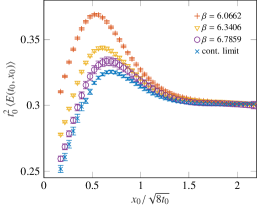
(a) Boundary peak for different lattice spacings at ${t=t_{0}}$.

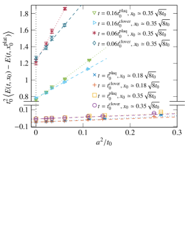
(b) Examples of continuum extrapolations at flow times ${t\in\{0.06,0.16,1\}t_{0}}$.

Figure 1: Action density near the time boundary for different flow times. On the right hand side, the continuum limit is taken by an extrapolation linearly in $a^{2}$, omitting O$(a)$ terms which in principle are present due to imprecisions of the boundary counterterms. The data supports their smallness.

3.2 Small flow-time expansion

Since $\left\langle E(t,x)\right\rangle$ in the boundary region has a smooth continuum limit, it can be used as a test case for the small flow-time expansion LuscherWeisz_PertFlow ; Luscher_FutureApplicationsFlow . More precisely the trace of the energy-momentum tensor $T_{\mu\mu}(x)$ can be extracted from the expansion of the action density LuscherWeisz_PertFlow ; Suzuki_EnergyMomentumTensor ; Ejiri_LatentHeat

$$E(t,x)=c_{\mathbf{1}}(t)+c_{E}(t)T_{\mu\mu}(x)+\mathrm{O}\left(t\right)\,,$$ (6)

with coefficients Suzuki_EnergyMomentumTensor

$$c_{\mathbf{1}}(t)=\left\langle E(t,x_{0}^{\text{plat}})\right\rangle\,,\,c_{E}(t)=\frac{1}{2b_{0}}\Big{(}1+2b_{0}\bar{s}\bar{g}^{2}+\mathrm{O}\left(\bar{g}^{4}\right)\Big{)}\,.$$ (7)

The definition of $c_{\mathbf{1}}(t)$ sets the vacuum expectation value of the trace to zero. The deviation of the action density at small flow time from its vacuum expectation value then yields

$$\left\langle T_{\mu\mu}(x_{0})\right\rangle=\lim_{t\rightarrow 0}\frac{1}{c_{E}(t)}\lim_{a\to 0}\left\langle E(t,x_{0})-E(t,x_{0}^{\text{plat}})\right\rangle\,.$$ (8)

The continuum limit and zero flow-time limit have to be performed in the correct order. Note that $\left\langle T_{\mu\mu}(x_{0})\right\rangle$ may be expressed as a Hilbert space off-diagonal matrix element between a $x_{0}$-dependent boundary state and the vacuum. This is qualitatively similar to the finite temperature application. The lattice data entering the extrapolations are restricted in flow time by Luscher_FutureApplicationsFlow

$$a\ll\sqrt{8t}\ll\text{relevant low energy scales}\,.$$ (9)

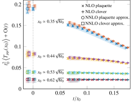
Figure 2: Trace of the energy-momentum tensor plus small flow-time corrections. Both discretizations, i.e., plaquette and clover are included, where the clover definition is overall shifted by $0.003$ in $t/t_{0}$ for readability. The coefficient $c_{E}(t)$ is known up to next to leading order. Uncertainties due to NNLO effects are estimated with eq. 10. Their effect is included in the error at zero flow time (shifted by $-0.01$ in $t/t_{0}$). The shaded areas mark the results of continuum extrapolations omitting one more lattice spacing.

As it turns out, discretisation effects are large for flow times $t\simeq 0.06t_{0}$ close to the boundary, where the matrix element is large. Hence the analysis has been restricted to $x_{0}\gtrsim 0.35\sqrt{8t_{0}}$ where a continuum extrapolation seems feasible, see figure 1(b). Depending on the chosen flow time, different numbers of lattice spacings $a\in[0.025,0.056]\,\text{fm}$ can be included into linear continuum extrapolations due to equation (9) and discretisation effects of higher order in the lattice spacing. Selected continuum extrapolated values at positive flow time are shown in fig. 2. Also the zero flow-time limit was performed. Figure 2 has been updated from the one shown at the conference, where correlations in $t$ were not yet included. As $c_{E}(t)$ is only known up to next to leading order (NLO) the NNLO effects are roughly estimated via

$$\Delta c_{E}(t)=\pm\frac{\bar{g}^{4}}{2b_{0}(4\pi)^{2}}=\pm\text{LO}\times\alpha^{2}\,.$$ (10)

The results show no significant impact of $\Delta c_{E}(t)$ on the zero flow-time limit at the available accuracy of ${10-20\,\%}$.

4 Step scaling for short distances and large volume

For six different lattice spacings $a$, Wilson loops have been measured with total statistic of $N_{\text{wl}}$, listed in table 1. The coupling $\overline{g}^{2}_{\rm qq}(r,a)$ at finite lattice spacing $a$ was derived from Wilson loops applying the analysis described in DetStat with only one difference: the parallel transporters in time are the dynamical gauge fields (no smearing) and statistical errors are reduced by the multi-hit technique Parisi .

To extrapolate the coupling to its continuum value we used two different strategies. In the regime of intermediate distances the scale was set at $r_{0}$ Sommer_parameter and the coupling $\overline{g}^{2}_{\rm qq}(r,a)$ was extrapolated to the continuum at $r/r_{0}=0.3,0.4,\dots,1.1$. In the short distance regime ($r\leq 0.45r_{0}$) the continuum extrapolation of the coupling $\overline{g}^{2}_{\rm qq}(r)$ was performed using step scaling.

Originally used to bridge large scale differences in finite volume couplings luscher1991numerical , we use it here to extrapolate from large to small distances, in large volume.

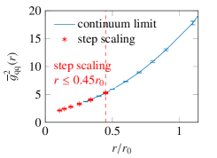
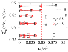
Figure 3: Six step scaling iterations starting from $r_{*}=0.45r_{0}$ reaching down to $r\approx 0.1r_{0}$ and the continuum limit for the large distance regime.

Figure 4: Continuum limit eq. 14 of the step scaling function with ($\rho\neq 0$) and without ($\rho=0$) slope. Red markers are shifted for visualization.

In an iterative process one computes the step scaling function

$$\overline{g}^{2}_{\rm qq}(sr)=\sigma(s,\overline{g}^{2}_{\rm qq}(r))\,,\quad s=0.75$$ (11)

with scale factor $s$. The step scaling function $\sigma$ is a discrete $\beta$ function. Starting at a given point $(\overline{g}^{2}_{\rm qq}(r_{*})=u_{0})$ a series is formed by applying the step scaling function iteratively:

$$u_{0} =\overline{g}^{2}_{\rm qq}(r_{*})\qquad r_{*}=0.45r_{0}$$

$$u_{1} =\overline{g}^{2}_{\rm qq}(sr_{*})=\sigma(s,u_{0})$$

$$u_{2} =\overline{g}^{2}_{\rm qq}(s^{2}r_{*})=\sigma(s,u_{1})$$

$$\qquad\vdots$$

$$u_{5} =\overline{g}^{2}_{\rm qq}(s^{5}r_{*})=\sigma(s,u_{4})$$

In this way one can reach down from $r_{*}=0.45r_{0}$ to $r_{5}=s^{5}r_{*}\approx 0.11r_{0}$, visualized in fig. 4. In each iteration one has to compute the lattice equivalent $\Sigma$ of the step scaling function, which has an additional dependence on the lattice spacing $a$,

$$\overline{g}^{2}_{\rm qq}(sr,a) =\Sigma(s,u,a/r)\left.\right|_{\overline{g}^{2}_{\rm qq}(r,a)=u}$$ (12)

and perform its continuum extrapolation,

$$\sigma(s,u)=\lim_{a/r\to 0}\Sigma(s,u,a/r)\,,$$ (13)

which is the starting point of the next iteration. The extrapolation to $a/r\to 0$ is performed as a linear fit

$$\Sigma(s,u,a/r)=\sigma(s,u)\{1+\rho\left(a/r\right)^{2}\}$$ (14)

with slope $\rho(u)$ and continuum value $\sigma(s,u)$. To test our treatment of cut off effects we extrapolate with and without slope $\rho$, where the extrapolation without slope is constrained to data points $(a/r)^{2}\leq 0.05$ close to the continuum. The two different extrapolations can be seen in fig. 4. The five different pairs of black solid and red dotted lines in fig. 4 show the fit of $\Sigma(s,u,a/r)$ scaled by $1/u$. The uppermost pair corresponds to the continuum extrapolation of the last iteration. Comparing the results for $\rho=0$ and $\rho\neq 0$, indicates that cut off effects are under good control. We use the ones with larger errors ($\rho\neq 0$) for further analysis.

In the small distance regime the step scaling strategy is beneficial in comparison to the traditional continuum limit, in which one would have to compute the coupling up to $r\geq r_{0}$. With step scaling the essential measurements on fine lattices involve only short distance quantities, where self-averaging works very well. This reduces computational requirements, less statistics is needed.

The continuum extrapolated non-perturbative values of $\sigma(s,u)$ can be compared to the prediction of perturbation theory. The latter are obtained by inserting the perturbative $\beta$-function into

$$\ln(s)=-\int\limits_{\sqrt{u}}^{\sqrt{\sigma(s,u)}}\frac{1}{\beta^{\rm qq}(g)}\operatorname{d}g$$ (15)

and solving for $\sigma(s,u)$. The comparison in fig. 5(a) shows surprisingly clear deviations from perturbation theory. The non-perturbative $\sigma(s,u)$ crosses the 4-loop prediction at around $u=3.5$ and is significantly lower for $u=2.4\,$.

5 The $\Lambda$-parameter

The $\Lambda$ parameter was calculated from lattice data

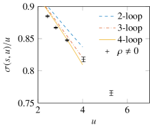
(a) The non-perturbative $\sigma(s,u)$ compared with its perturbative equivalent up to four loop order.

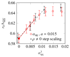
(b) Extrapolation of the $\Lambda$ parameter from the 4-loop $\beta$-function in the qq-scheme.

Figure 5: The running of the coupling and the $\Lambda$-parameter.

$$\Lambda_{{\rm qq}}=\varphi(\overline{g}_{\rm qq}(r))/r\,,\qquad\varphi(\overline{g}_{\rm qq}(r))=(b_{0}\overline{g}_{\rm qq}^{2})^{-\frac{b_{1}}{2b_{0}^{2}}}\mathrm{e}^{-\frac{1}{2b_{0}\overline{g}_{\rm qq}^{2}}}\times\exp{\left[-\int\limits_{0}^{\overline{g}_{\rm qq}}\,{\rm d}{x}\left(\frac{1}{\beta^{\rm qq}(x)}+\frac{1}{b_{0}x^{3}}-\frac{b_{1}}{b_{0}^{2}x}\right)\right]}$$ (16)

using the perturbative $\beta$-function at 4-loop order. As a Renormalization Group Invariant the $\Lambda$-parameter should not change as we vary $\overline{g}^{2}_{\rm qq}(r)$. Of course this only holds true in a regime where the 4-loop approximation of $\beta^{({\rm qq})}$ is sufficiently accurate, i.e. the coupling is sufficiently small. We have apparently not reached this region, but by extrapolating the last three values of $r_{0}\Lambda_{\overline{\rm{MS}}}$ to $\overline{g}_{\rm qq}\to 0$ it is possible to determine the non-perturbative value of $\Lambda_{\overline{\rm{MS}}}$. Figure 5(b) shows the extrapolation

$$r_{0}\Lambda_{{\rm qq}}=r_{0}\lim_{\begin{subarray}{c}r\to 0\\ (\overline{g}_{\rm qq}\to 0)\end{subarray}}\varphi(\overline{g}_{\rm qq}(r))/r$$ (17)

for the coupling $\alpha_{\rm qq}(r)=\overline{g}^{2}_{\rm qq}(r)/4\pi$ in the continuum and at finest lattice spacing.

The last three points are used to extrapolate linearly to $\alpha_{\rm qq}=0$. The final result $r_{0}\Lambda_{\overline{\rm{MS}}}=0.590(16)$ is from the $\rho\neq 0$ extrapolation shown in fig. 5(b), taking also the results with $\rho=0$ into account to estimate the final range.

At $\alpha_{\rm qq}=0.24$ ($\alpha_{\rm qq}^{3}\approx 0.014$), the result $r_{0}\Lambda_{\overline{\rm{MS}}}^{\text{4-loop}}$ deviates significantly from the extrapolated value. A similar observations was made in PhysRevLett.117.182001 at $\alpha=0.19$ in a different non-perturbative renormalization scheme.

6 Conclusion

Open boundary conditions prevent topological freezing when simulating fine lattice spacings. This allows the measurement of short distance and small flow-time quantities up to a regime, in which one can test perturbation theory and the small flow-time expansion. We computed the coupling in the qq-scheme down to about $\alpha_{\mathrm{qq}}=0.2$. Extracting the $\Lambda$-parameter from these coupling values using the four loop $\beta$-function still showed a significant dependence on $\alpha$. Linear extrapolation in the (perturbatively) dominating correction term $\alpha^{3}$ yielded our estimate

$$r_{0}\Lambda_{\overline{\rm{MS}}}=0.590(16)\,.$$ (18)

It is in agreement with the FLAG average Aoki:2013ldr but has a smaller error. The extrapolation to $\alpha=0$ in figure 5(b) pushes our estimate some 1-2 standard deviations below previous pure gauge theory results Brambilla:2010pp ; Gockeler:2005rv with small errors.

Our investigation of the behaviour of $\left\langle E(t,x_{0})\right\rangle$ near the open boundary showed that effects are noticeable up to a distance of about $x_{0}=\sqrt{20t_{0}}$ ($\approx 0.8$fm), roughly independent of the lattice spacing. Hence boundary improvement will not appreciably enlarge the usable fraction of lattices with open boundary conditions.

As a proof of concept we studied the small flow-time limit of the action density near the boundary. As $t\to 0$ it yields a matrix element of the trace of the energy momentum tensor. The expected linear behaviour in $t$ is indeed found and the zero flow-time limit seems feasible. Hence the method can be applied, e.g. for finite temperature physics Ejiri_LatentHeat ; Suzuki_EnergyMomentumTensor . Due to the distinct discretisation effects at small flow time as well as a significant $t$-dependence, we do find that continuum extrapolation and $t\to 0$ extrapolation are necessary – of course in the correct order. Note that for $\alpha_{\mathrm{qq}}$ we had lattice spacings as small as $a=0.015\,\mathrm{fm}$, while for the small flow-time expansion we only went down to $a=0.025\,\mathrm{fm}$ so far.

References

- (1) S. Schaefer, R. Sommer, F. Virotta (ALPHA), Nucl. Phys. B845, 93 (2011), 1009.5228
- (2) M. Lüscher, PoS LATTICE2010, 015 (2010), 1009.5877
- (3) M. Lüscher, S. Schaefer, Journal of High Energy Physics 7, 36 (2011), 1105.4749
- (4) M. Bruno, S. Schaefer, R. Sommer (ALPHA), JHEP 08, 150 (2014), 1406.5363
- (5) M. Lüscher, P. Weisz, JHEP 02, 051 (2011), 1101.0963
- (6) Shinji Ejiri et al., Determination of latent heat at the finite temperature phase transition of SU(3) gauge theory, in Proceedings, 34th International Symposium on Lattice Field Theory (Lattice 2016) (2017), 1701.08570
- (7) M. Peter, Nucl. Phys. B501, 471 (1997), hep-ph/9702245
- (8) Y. Schroder, Phys. Lett. B447, 321 (1999), hep-ph/9812205
- (9) C. Anzai, Y. Kiyo, Y. Sumino, Phys. Rev. Lett. 104, 112003 (2010), 0911.4335
- (10) A.V. Smirnov, V.A. Smirnov, M. Steinhauser, Phys. Rev. Lett. 104, 112002 (2010), 0911.4742
- (11) N. Brambilla, A. Pineda, J. Soto, A. Vairo, Nucl. Phys. B566, 275 (2000), hep-ph/9907240
- (12) K.G. Wilson, Phys. Rev. D 10, 2445 (1974)
- (13) N. Cabibbo, E. Marinari, Physics Letters B 119, 387 (1982)
- (14) M. Creutz, Phys. Rev. D 36, 515 (1987)
- (15) F.R. Brown, T.J. Woch, Phys. Rev. Lett. 58, 2394 (1987)
- (16) S.L. Adler, Phys. Rev. D 37, 458 (1988)
- (17) S. Necco, R. Sommer, Nuclear Physics B 622, 328 (2002), hep-lat/0108008
- (18) M. Lüscher, JHEP 08, 071 (2010), [Erratum: JHEP03,092(2014)], 1006.4518
- (19) B. Sheikholeslami, R. Wohlert, Nucl. Phys. B259, 572 (1985)
- (20) M. Lüscher, Future applications of the Yang-Mills gradient flow in lattice QCD, in Proceedings, 31st International Symposium on Lattice Field Theory (Lattice 2013): Mainz, Germany, July 29-August 3, 2013 (2014), Vol. LATTICE2013, p. 016, 1308.5598
- (21) H. Suzuki, PTEP 2013, 083B03 (2013), [Erratum: PTEP2015,079201(2015)], 1304.0533
- (22) M. Donnellan, F. Knechtli, B. Leder, R. Sommer, Nucl. Phys. B849, 45 (2011), 1012.3037
- (23) G. Parisi, R. Petronzio, F. Rapuano, Physics Letters B 128, 418 (1983)
- (24) R. Sommer, Nucl. Phys. B411, 839 (1994), hep-lat/9310022
- (25) M. Lüscher, P. Weisz, U. Wolff, Nuclear Physics B 359, 221 (1991)
- (26) M. Dalla Brida, P. Fritzsch, T. Korzec, A. Ramos, S. Sint, R. Sommer (ALPHA Collaboration), Phys. Rev. Lett. 117, 182001 (2016)
- (27) S. Aoki et al., Eur. Phys. J. C74, 2890 (2014), 1310.8555
- (28) N. Brambilla, X. Garcia i Tormo, J. Soto, A. Vairo, Phys. Rev. Lett. 105, 212001 (2010), [Erratum: Phys. Rev. Lett.108,269903(2012)], 1006.2066
- (29) M. Gockeler, R. Horsley, A.C. Irving, D. Pleiter, P.E.L. Rakow, G. Schierholz, H. Stuben, Phys. Rev. D73, 014513 (2006), hep-ph/0502212