Capacity Upper Bounds for Deletion-Type Channels

Abstract

We develop a systematic approach, based on convex programming and real analysis, for obtaining upper bounds on the capacity of the binary deletion channel and, more generally, channels with i.i.d. insertions and deletions. Other than the classical deletion channel, we give a special attention to the Poisson-repeat channel introduced by Mitzenmacher and Drinea (IEEE Transactions on Information Theory, 2006). Our framework can be applied to obtain capacity upper bounds for any repetition distribution (the deletion and Poisson-repeat channels corresponding to the special cases of Bernoulli and Poisson distributions). Our techniques essentially reduce the task of proving capacity upper bounds to maximizing a univariate, real-valued, and often concave function over a bounded interval. The corresponding univariate function is carefully designed according to the underlying distribution of repetitions and the choices vary depending on the desired strength of the upper bounds as well as the desired simplicity of the function (e.g., being only efficiently computable versus having an explicit closed-form expression in terms of elementary, or common special, functions). Among our results, we show the following:

1. The capacity of the binary deletion channel with deletion probability $d$ is at most $(1-d)\log\varphi$ for $d\geq 1/2$, and, assuming the capacity function is convex, is at most $1-d\log(4/\varphi)$ for $d<1/2$, where $\varphi=(1+\sqrt{5})/2$ is the golden ratio. This is the first nontrivial capacity upper bound for any value of $d$ outside the limiting case $d\to 0$ that is fully explicit and proved without computer assistance.

2. We derive the first set of capacity upper bounds for the Poisson-repeat channel. Our results uncover further striking connections between this channel and the deletion channel, and suggest, somewhat counter-intuitively, that the Poisson-repeat channel is actually analytically simpler than the deletion channel and may be of key importance to a complete understanding of the deletion channel.

3. We derive several novel upper bounds on the capacity of the deletion channel. All upper bounds are maximums of efficiently computable, and concave, univariate real functions over a bounded domain. In turn, we upper bound these functions in terms of explicit elementary and standard special functions, whose maximums can be found even more efficiently (and sometimes, analytically, for example for $d=1/2$).

Along the way, we develop several new techniques of potentially independent interest. For example, we develop systematic techniques to study channels with mean constraints over the reals. Furthermore, we motivate the study of novel probability distributions over non-negative integers as well as novel special functions which could be of interest to mathematical analysis.

Keywords: Coding theory, Synchronization error-correcting codes, Channel coding.

1 Introduction

The binary deletion channel is generally regarded as the simplest model for communication in presence of synchronization errors. In this model, a transmitter encodes messages as a (potentially unbounded) stream of bits which is then sent to a receiver over a communications channel. The channel does not corrupt bits. However, each bit may be independently discarded by the channel with a deletion probability $d\in[0,1)$. The receiver receives the sequence of undiscarded bits, in their respective order, and has to reconstruct the sent message with vanishing failure probability. Despite the remarkable simplicity of this fundamental model of communication, the capacity of the deletion channel; i.e., the maximum achievable transmission rate, remains unknown. Apart from the obvious significance in information, coding, and communications theory, the problem has attracted significant attention from the theoretical computer science community (e.g., [ref:Mit09, ref:SZ99, ref:GNW12, ref:GW17, ref:BGZ16, ref:BGH17]). This is due to the problem’s rich combinatorial structure and its fundamental connection with the understanding of the distribution of long subsequences in bit-strings, which, in turn, is of significance to such theory problems as pattern matching, edit distance, longest common subsequence, communication complexity problems involving the edit distance, the document exchange problem (cf. [ref:BZ16]) or secure sketching in cryptography [ref:DORS08], to name a few. It is also closely related to the algorithmic trace reconstruction problem which, in turn, is of significance to real world applications ranging from sensor networks to computational biology [ref:Mit09].

1.1 Previous work

There is already a relatively vast literature on the deletion channel problem, and we are only able to touch upon some of the major results most relevant to this work. Qualitatively, it is known that i) the capacity curve for this channel is continuous, ii) the capacity is positive for all $d\in[0,1)$ [ref:DG01, ref:DG06], iii) the capacity is $1-\Theta(d\log d)$ (as in the binary symmetric channel) when $d\to 0$ [ref:KMS10, ref:KM13] and $\Theta(1-d)$ when $d\to 1$ (as in the binary erasure channel) [ref:DM07, ref:MD06, ref:Dal11]. Trivially, the capacity is at most the capacity of the binary erasure channel; i.e., $1-d$. Nevertheless, the exact capacity of the channel remains elusive. A related problem is to identify the best achievable rate against adversarial, or oblivious, deletions; for which significant progress has been recently made [ref:BGH17, ref:GR18]. However, in this work we focus on the Shannon-type capacity over random deletions (and, more generally, repetitions). Much of the major known results on the subject as well as the significance to theoretical computer science are discussed in Mitzenmacher’s excellent survey [ref:Mit09].

On the achievability side, Diggavi and Grossglauser [ref:DG01, ref:DG06] were the first to show that the capacity of the deletion channel is nonzero for all $d\in[0,1)$. A more explicit capacity lower bound of (slightly better than) $(1-d)/9$, for all $d$, was proved by Drinea and Mitzenmacher [ref:DM07, ref:MD06], where in the latter work they also introduced and motivated the Poisson-repeat channel. This channel not only deletes bits but may also insert replicated bits in the stream. More precisely, the channel is defined by a parameter $\lambda$ and, given a bit, replicates the bit by a number sampled from a Poisson distribution with mean $\lambda>0$ (the bit is deleted if the number of repetitions is zero). In [ref:MD06], the authors establish a connection between the Poisson-repeat and the deletion channel. Namely, they show that any lower bound on the capacity of any Poisson-repeat channel translates into a capacity lower bound for any deletion channel. Using a first-order Markov chain for generating the input distribution, and numerical computations on the resulting capacity bound expressions for various choices of $\lambda$, they derive the claimed capacity lower bound of $(1-d)/9$ for the deletion channel.

For small deletion probability $d\to 0$, several results show that the deletion capacity behaves similar to the symmetric channel. Combined with [ref:Gal61, ref:Zig69, ref:DG06], Kalai, Mitzenmacher, and Sudan [ref:KMS10] show that in this regime that capacity is $1-h(d)(1-o(1))$, where $h(\cdot)$ is the binary entropy function. Independently of this work, and based on a parameter continuity argument, Kanoria and Montanari [ref:KM13] obtain a more refined asymptotic estimate in this regime that is correct up to the $O(d)$ term.

Diggavi, Mitzenmacher and Pfister [ref:MDP07] obtained capacity upper bounds for all $d$, including the first nontrivial upper bound, of $0.7918(1-d)$, for $d\to 1$. To show the upper bounds, they consider a genie-aided decoder with access to side information about the deletion process, and then upper bound the capacity of the channel with side information (which is higher than the original capacity) using a combination of classical information theoretic tools and a computer-based distribution-optimization component. Different sets of numerical capacity upper bounds were obtained in [ref:FD10] (and for more general channels in [ref:FDE11]) based on several, carefully designed, genie-aided decoders. These constructions essentially reduce the problem to upper bounding the capacity of a finite variation of the deletion channel problem, whose capacity is in turn numerically computed using the Arimoto-Blahut algorithm (which runs in exponential time in the finite number of bits). Both [ref:MDP07] and [ref:FD10] thus cleverly identify a finite-domain capacity problem, that is solved numerically, and then upper bound the deletion capacity using the numerical results for the finite problem. Such techniques cannot be readily extended to such problems as the Poisson-repeat channel problem which are inherently infinite.

1.2 Our main contributions

Roughly speaking, the techniques of [ref:MDP07] and [ref:FD10] pursue the following recipe: i) “enhance” the channel to one with a higher capacity by carefully considering a “genie-aided” decoder that receives auxiliary information from the channel; ii) Heuristically extract a finite optimization problem to upper bound the capacity of the enhanced (and thus the original) channel; iii) Numerically solve the finite optimization problem by a computer. While the above general method results in very strong capacity upper bounds, much of the mathematical structure of the problem is pushed into the computationally intensive numerical optimization problem in the third step. It is thus unclear to what extent can the methods be further developed towards a complete understanding of the channel capacity. In this work, rather than setting our goal to improving the best known numerical capacity upper bounds for the deletion channel, we focus on gaining deeper insights about the analytic structure of the problem (nevertheless, as a proof of concept, we are able to improve the best reported numerical upper bounds for small deletion probability; e.g., for $d\leq 0.02$). We develop several tools that further the existing intuitions on the deletion channel problem and may potentially serve as key steps towards a full characterization of the capacity. As a result, we are able, for the first time, to develop a single and systematic method that results in a capacity upper bound curve for the deletion channel which is smooth, convex-shaped, non-trivial for all $d$, and simultaneously exhibits the correct behavior of $c(1-d)$, for a constant $c<1$, at $d\to 1$ and $1-\Theta(h(d))$ at $d\to 0$ (see Figure 16). The fact that our approach obtains the above features in a natural and organic way suggests that the true capacity of the deletion channel might have the same qualitative shape as what we obtain.

As discussed above, the best known reported capacity upper bounds for the deletion channel [ref:FD10, ref:MDP07, ref:RD15], are based on identifying a finite, but as large as possible, sub-problem (possibly by adding side information) and then searching for the optimum solution for the finite problem by a computer. In contrast, a key focus in our work is to avoid any computer-assisted components in the proofs as much as possible, so as to gain as much intuition about the mathematical structure of the problem as possible. Our results, including all the involved distributions in the proofs, are indeed fully analytical. Namely, we upper bound the capacity of the deletion channel as the maximum of a univariate real function, which is concave and smooth, over the interval $(0,1)$ (depicted in Figure 14). The function to be maximized is explicitly defined in terms of exponentially decaying sums, and is thus computable in polynomial time in the desired accuracy. If desired, computation of the involved sums can be avoided by using the sharp upper and lower bound estimates on the function that we provide in terms of both elementary and standard special functions (Figure 15). The only numerical computation would thus involve finding the maximum value of an explicitly defined concave function over $(0,1)$. Even this can be avoided in some cases, leading us to the first fully explicit capacity upper bound for the deletion channel that is nontrivial for all deletion probabilities $d\in(0,1)$ and proved without any numerical computation: The deletion capacity is at most $(1-d)\log\varphi$ for $d\geq 1/2$, and, under the plausible conjecture that the capacity function is convex [ref:Dal11], at most $1-d\log(4/\varphi)$ for $d<1/2$, where $\varphi=(1+\sqrt{5})/2$ is the golden ratio. We remark that this, itself, is better than the bounds reported in [ref:MDP07] for all $d\geq 0.70$, while our numerical bounds improve those of [ref:MDP07] for all $d\geq 0.35$.

In addition to the classical deletion channel, our methods are generally applicable to any channel with independent insertions and deletions defined by any given repetition rule. Namely, given an arbitrary (possibly infinite) distribution $\mathcal{D}$ on non-negative integers, our methods can be applied to upper bound the capacity of a channel—what we call a $\mathcal{D}$-repeat channel, that replaces each input bit independently with a number of repetitions sampled from $\mathcal{D}$ (where the outcome zero would cause deletion of the bit). For the deletion channel, $\mathcal{D}$ would be a known Bernoulli distribution.

For such problems as the Poisson-repeat channel problem, introduced by Mitzenmacher and Drinea [ref:MD06], that are inherently infinite (even if only one bit is supplied at the input), the known methods [ref:FD10, ref:MDP07] cannot be readily used, since it is not clear how to identify a finite sub-problem that can be optimized by a computer-based search. In contrast, we show that our method easily applies to the Poisson-repeat channel (where $\mathcal{D}$ is Poisson with a known mean $\lambda$), and thus we obtain the first set of capacity upper bounds for this channel. Our methods demonstrate striking connections between the analytical structure of this channel and the deletion channel, and suggest that understanding the Poisson-repeat channel may be the key towards the ultimate characterization of the capacity of the deletion channel. Even though the Poisson-repeat channel may appear more complex than the deletion channel (since it not only deletes, but also inserts bits), our results suggest that the Poisson-repeat channel may be simpler to analyze. This is mainly due to the fact that an $x$-fold convolution of $\mathcal{D}$ with itself is a binomial distribution for the deletion channel, which is a more complex distribution than Poisson, and indeed, contains the latter as a limiting special case. In fact, we study the Poisson-repeat channel first, which then naturally guides us towards our results for the deletion channel. Our obtained bounds for both channels are plotted in Figures 9 and 16 and tabulated in Tables B.5 and B.5.

To obtain our results, we develop a number of techniques along the way that may be of independent interest. We motivate a systematic study of what we call general mean-limited channels, and their special case of convolution channels. These are channels, with input and output alphabets over the reals, defined by a known probability transition rule and a mean-constraint on their output distributions. Special cases include the mean-limited binomial and Poisson channels, that model how the deletion and Poisson-repeat channels shrink consecutive runs of bits. The notion and our techniques can be used to model physical channels studied outside the context of deletion-type channels as well, a notable example being the well-known Poisson channel that is of central importance to optical communications systems [ref:Sha90]. Indeed, a subsequent work by the author [ref:CR18] successfully applies the techniques developed in this work to obtain improved upper bounds on the capacity of the discrete-time Poisson channel. Furthermore, our contributions in probability theory include motivating novel distributions over non-negative integers and a first study of them, which may be of use in other contexts as well. This includes what we define as an “inverse binomial” distribution, as well as distributions obtained by multiplying the probability mass function of the Poisson distribution $p(y)$ by $y^{y}$ or $\exp(yH_{y-1})$, where $H$ denotes harmonic numbers (see (43) and (52)). We introduce novel special functions to study such distributions (e.g., generalizations of the log-gamma function; see (112)) which may be of independent interest to mathematical analysis.

Organization

The rest of the article is organized as follows: Section 2 gives a high-level exposition of the entire work, explaining the developed techniques with a focus on intuitions and underlying insights rather than the technical details. In Section 3, we formally define the notion of general mean-limited channels, as well as the special case of convolution channels. We prove a duality-based necessary and sufficient condition for achieving the capacity of such channels, as well as the dual feasibility criteria that certify upper bounds on the capacity. Section 4 formally defines the general notion of $\mathcal{D}$-repeat channels, and proves a capacity upper bound for such channels based on the capacity of a mean-limited channel defined according to $\mathcal{D}$. We use the obtained tools in Section 5 to obtain our capacity upper bounds for the Poisson-repeat channel. Towards this end, we construct two dual-feasible solutions for the corresponding mean-limited channel and estimate their parameters in terms of elementary and standard special functions. In Section 6, guided by the result obtained for the Poisson-repeat channel, we prove our capacity upper bounds for the deletion channel. We first introduce the notion of inverse binomial distributions, and then show that it is dual feasible for the mean-limited binomial channel. We estimate the parameters of this distribution in terms of elementary and standard spacial functions. We then apply a truncation technique, that we first develop for Poisson-repeat channels, to refine the dual feasible solution and obtain improved capacity upper bounds.

Notation

Unless otherwise stated, all logarithms are taken to base $e$, and the measure of information is converted from nats to bits only for the final numerical estimates. We denote the set of non-negative real numbers by $\mathbb{R}^{\geq 0}$ and the set of non-negative integers by $\mathds{N}^{\geq 0}$. As is standard in information theory, we generally use capital letters for random variables. When there is no risk of confusion, we may use the same symbol for a random variable and its underlying distribution. Support of a random variable $X$, denoted by $\mathsf{supp}(X)$, is the set of the possible outcomes of $X$. Calligraphic letters are used for several purposes; alphabets, distributions, and probability transition rules. The entropy of a random variable $X$ is denoted by $H(X)$, and $h(p)$ denotes the binary entropy function:

$$h(p):=-p\log p-(1-p)\log(1-p).$$

The Kullback-Leibler (KL) divergence between the underlying distributions of random variables $X$ and $Y$, denoted by $D_{\mathsf{KL}}({X}\|{Y})$, is defined as

$$D_{\mathsf{KL}}({X}\|{Y}):=\sum_{x\in\mathsf{supp}(X)}\Pr[X=x]\log(\Pr[X=x]/\Pr[Y=x]).$$

We use $I(X;Y)$ for the mutual information between jointly distributed random variables $X$ and $Y$, and $I(X;Y|Z)$ for the conditional mutual information given a third variable $Z$. We use the asymptotic notation $f(x)\sim g(x)$ to mean $\lim_{x\to\infty}f(x)/g(x)=1$. The binomial distribution with $x$ trials and success probability $p$ is denoted by ${\mathsf{Bin}}_{x,p}$, and the Bernoulli distribution with mean $p$ is denoted by ${\mathsf{Ber}}_{p}$. The capacity of a channel $\mathsf{Ch}$ is denoted by ${\mathsf{Cap}}(\mathsf{Ch})$. We may use the binomial coefficient $\binom{x}{y}$ over non-integers, in which case the definition $\binom{x}{y}:=\Gamma(1+x)/(\Gamma(1+y)\Gamma(1+x-y))$ should be used.

2 High-level exposition of the techniques and results

In this work, we formalize and study the notion of “general repeat channels”, which are binary input channels characterized by a given probability distribution $\mathcal{D}$ over non-negative integers. A $\mathcal{D}$-repeat channel, given a bit, draws an independent sample $D\geq 0$ from $\mathcal{D}$ and outputs $D$ copies of the received bit. We define the deletion probability $d$ of the channel to be the probability that $\mathcal{D}$ assigns to zero, and let $p=p(\mathcal{D}):=1-d$ be the retention probability. Thus, what we call the deletion channel corresponds to the case where $\mathcal{D}$ is the Bernoulli distribution with mean $p$. On the other hand, if $\mathcal{D}$ is a Poisson distribution with mean $\lambda$, we get a Poisson-repeat channel with deletion probability $d=e^{-\lambda}$. We note that, in general, $\mathcal{D}$ need not be uniquely determined by its deletion parameter $d$, albeit this is the case for the class of deletion and Poisson-repeat channels.

2.1 Reduction to mean-limited and convolution channels

Suppose the input to a $\mathcal{D}$-repeat channel is a bit-sequence $X={B_{1}},{B_{2}},\ldots,{B_{n}}$ with $Y$ being the output bit-sequence. If $\mu:=\mathds{E}[\mathcal{D}]$, the expected output length would be $\mu n$. By Shannon’s theorem, it can be seen (as in [ref:Dob67]) that the capacity of the channel, that we denote below by ${\mathsf{Cap}}(\mathcal{D})$, is the supremum of the normalized mutual information between $X$ and $Y$; i.e., ${\mathsf{Cap}}(\mathcal{D})=\lim_{n\to\infty}{I(X;Y)}/n$.

A common technique in analyzing the deletion channel is to consider how it acts on runs of bits, rather than the individual bits. Given a run of $x>0$ bits, the deletion channel outputs a run of ${\mathsf{Bin}}_{x,p}$ bits; i.e., a sample from the binomial distribution with $x$ trials and success probability $p$. For the Poisson-repeat channel, this would be a run of length given by a Poisson sample with mean $\lambda x$. In general, the distribution of the output run-length would be the $x$-fold convolution of $\mathcal{D}$ with itself, that we denote by $\mathcal{D}^{\oplus x}$.

Since $n$ grows to infinity, without loss of generality, we can assume that the first input bit $B_{1}$ is zero. This allows us to unambiguously think of $X$ as its run-length encoding $X={X_{1}},{X_{2}},\ldots,{X_{t}}$, where each $X_{i}$ is a positive integer. Similarly, we may also think of $Y$ by its run-length encoding $Y={Y_{1}},{Y_{2}},\ldots,{Y_{m}}$, where each $Y_{i}$ is a positive integer. This will identify $Y$ up to a negation of all bits. Since the channel has memory, the random variables $Y_{i}$ (unconditionally) are not necessarily independent. However, this would be the case if the $X_{i}$ are independent and identically distributed, in which case the $Y_{i}$ also become identically distributed. Note that, given $X$, the bit-length of $Y$ and the parameter $m$ are random variables determined by the channel, and indeed the randomness of $m$ causes technical difficulties that should be rigorously handled by a careful analysis. However, in the informal exposition below we pretend that $m$ is known and fixed a priori. One may now attempt to use the chain rule and write

$$I(X;Y)=I(X;Y_{1})+I(X;Y_{2}|Y_{1})+\cdots+I(X;Y_{m}|Y_{1}\ldots Y_{m-1})\leq\sum_{i=1}^{m}(H(Y_{i})-H(Y_{i}|X,Y_{1}\ldots Y_{m-1})).$$

A major difficulty in deriving the capacity of the deletion channel is the fact that, unlike channels with no synchronization errors, a certain $Y_{i}$ does not only depend on the corresponding $X_{i}$, but rather, potentially any part of $X$. Given $X$, we know that $Y_{i}$ has a binomial distribution with mean depending on the summation $X_{J}+X_{J+2}+\cdots+X_{J+2K}$, for some random variables $J$ and $K$ that are in general difficult to analyze. Furthermore, even given a fixed $X$, the random variables $Y_{1},Y_{2},\ldots$ do not become conditionally independent. Therefore, the above result of the chain rule cannot be upper bounded by a simpler, single-letter, expression. A natural idea, that has been pursued previously (e.g., [ref:MDP07, ref:FD10]), is to consider “genie-aided” decoders that receive enhanced side information by the channel. The side information is carefully designed so as to reduce the problem to an i.i.d. channel problem that can be analyzed more conveniently. However, this approach generally comes at the expense of effectively turning the channel into one with strictly higher capacity, and consequently, obtaining inherently sub-optimal capacity upper bounds.

The result of Diggavi, Mitzenmacher, and Pfister [ref:MDP07].

An elegant execution of the above idea, that in fact inspires the starting point of our work, has been done in [ref:MDP07] which we briefly explain here. This result is based on the simple idea that, if we imagine that the channel places a “comma” after each run of bits, such that the commas are never deleted by the channel, this can only increase the capacity. Furthermore, the enhanced channel is equivalent to an i.i.d. channel that receives a stream of positive integers (i.e., the run-length encoding of $X$) and passes each integer independently over a “run-length” channel. The effect of the run-length channel, given an input $x$, is to output a sample from ${\mathsf{Bin}}_{x,1-d}$; i.e., the binomial distribution with $x$ trials and success probability $p=1-d$. Now, the capacity of the deletion channel can be upper bounded by the capacity of the run-length channel, normalized by the number of input channel uses (i.e., the length of $X$). Since the run-length channel is i.i.d., its capacity is equivalent to the single-letter capacity. Thus, letting $U$ and $V$ denote the input and output of a single use of the run-length channel, capacity of the deletion channel is upper bounded by $\sup_{U}I(U;V)/\mathds{E}[U]$, where the supremum is over the distribution of $U$ over positive integers. At this point, a fundamental result of Abdel-Ghaffar [ref:AG93] on per-unit-cost capacity can be used to, in turn, upper bound the resulting expression.

In the per-unit-cost capacity problem, a cost function $c(u)$ is defined over the input domain $\mathcal{U}$ of a channel with transition rule $\mathcal{P}(v|u)$ and the capacity is defined as $\sup I(U;V)/\mathds{E}[c(U)]$, where the supremum is over the distribution of $U$. For the above application, the input domain is the positive integers and the cost function is identity: $c(u)=u$. As proved in [ref:AG93], a necessary and sufficient condition for a pair $(U,V)$ to be capacity achieving is the following: Letting

$$C(V):=\sup_{u\in\mathcal{U}}(D_{\mathsf{KL}}({V_{u}}\|{V})/c(u)),$$

where $V_{u}$ is the output distribution corresponding to a fixed input $u$ and $D_{\mathsf{KL}}({\cdot}\|{\cdot})$ is the Kullback-Leibler (KL) divergence, the supremum is attained for all $u$ on the support of $U$. In this case, $C(V)$ is the per-unit-cost capacity. Furthermore, for any distribution $V$ on the output domain (whether or not it corresponds to an input distribution), the capacity is upper bounded by $C(V)$ as defined above.

There are two drawbacks with the above approach taken by [ref:MDP07]. First, the side information in fact genuinely increases the channel’s capacity, and therefore, the upper bounds resulting from this method are inherently sub-optimal. One way to see this is to consider the case where $p=1-d$ is small. Consider the run-length channel $(U,V)$ and a choice of $U$ that assigns a $1-p$ of the probability mass to $U=1$, and the rest to $U=2$. In this case, one can see that $I(U;V)=\Omega(p\log(1/p))$, and thus, the per-unit-cost capacity is also at least $\Omega(p\log(1/p))$. This is while, by the trivial erasure channel upper bound, the deletion capacity must be at most $p$. Indeed, the numerical upper bounds reported by [ref:MDP07] exhibit this phenomenon at $d$ close to one (notice the distinctive concavity in this area in Figure 16). The second drawback is that, while the result of Abdel-Ghaffar is in principle powerful enough to characterize the true per-unit-cost capacity upper bound, it may be extremely difficult to work with this result analytically. A way around this issue, undertaken in [ref:MDP07], is to employ a computer-based search. In order to do so, first a finite-domain distribution (supported up to an integer $M$) for $U$ that maximizes the capacity is constructed by a computer-based search, and the corresponding KL divergence supremum, up to $M$, is numerically computed. Then, the resulting $V$ is truncated and the tail is geometrically redistributed over the remaining (infinite) input domain. The KL divergence at large values of $u$ can be accurately approximated by a linear function of $u$, at which point [ref:AG93] can be applied with the modified choice of $V$, allowing the resulting capacity upper bound to be numerically computed. While this approach indeed achieves very strong numerical capacity upper bounds (especially for small to moderate values of $d$), much of the analytic structure of the problem is absorbed by the computer-based search, making further progress elusive. In this work, we develop a systematic, albeit technically demanding, approach to overcome the barriers encountered by [ref:MDP07].

Equivalent reformulation of the channel.

Consider any $\mathcal{D}$-repeat channel $\mathsf{Ch}$ with deletion probability $d=1-p$. Rather than introducing side information, which, as demonstrated above, may result in a channel with strictly larger capacity, we use a careful analysis to decompose the action of the channel into two steps, forming a Markov chain $X-Z-Y$, such that the resulting $Y$ from the two-step process has the exact distribution as the run-length encoding of the output of $\mathsf{Ch}$. Then, we upper bound the capacity by $I(Z;Y)$ divided by the number of channel uses in $X$. Assume, without loss of generality, that the first input bit in $X$ is zero and this bit is promised not to be deleted by the channel (in particular, the first bit ever output by the channel is also zero). Given the input $X$, the channel considers the run-length encoding ${X_{1}},{X_{2}},\ldots,{X_{t}}$ of $X$. In order to produce the first run in the output, the channel starts deleting bits from the even runs ${X_{2}},{X_{4}},\ldots$ until the first non-deletion event occurs, say at run $X_{2j}$. The odd runs are then combined as $Z_{1}=X_{1}+X_{3}+\cdots+X_{2j-1}$, and the process continues from the first survived bit in the even runs until the input is fully scanned. The resulting sequence ${Z_{1}},{Z_{2}},\ldots,{Z_{m}}$ is then passed component-wise through a channel $\mathsf{Ch}^{\prime}$, with integer input and output, defined according to $\mathcal{D}$, to produce the output sequence ${Y_{1}},{Y_{2}},\ldots,{Y_{m}}$ (for the case of the deletion channel, each $Y_{i}$ is formed simply by passing $Z_{i}-1$ through a binomial channel, much similar to [ref:MDP07]). We show that the resulting sequence has precisely the same distribution as the run-length encoding of the output of $\mathsf{Ch}$. By a delicate analysis of this process, which is depicted in Figure 1, we are able to show that the capacity of $\mathsf{Ch}$ is upper bounded as

$${\mathsf{Cap}}(\mathsf{Ch})\leq\sup_{U}\frac{I(U;V)}{1/p+\mathds{E}[U]},$$ (1)

where $U$ and $V$ are the input and output distributions of $\mathsf{Ch}^{\prime}$. This constitutes the first technical building block in our capacity upper bound proofs. The bound (1) has a similar flavor in form, but is strictly stronger, than the upper bound expression in [ref:MDP07] (especially for larger $d$).

Mean-limited and convolution channels.

Once (1) is available, one may attempt to apply Abdel-Ghaffar’s result [ref:AG93] to obtain a capacity upper bound, by using the cost function $c(u)=u+1/p$. Indeed, any upper bound may in principle be obtained by this result as it provides necessary and sufficient conditions for characterizing the quantity on the right hand side of (1). However, as demonstrated by [ref:MDP07], an analytic approach for obtaining a distribution $V$ that minimizes the divergence fraction $\sup_{u\in\mathcal{U}}D_{\mathsf{KL}}({V_{u}}\|{V})/(u+1/p)$, or even gets sharply close to the minimum, may be extremely challenging. Instead, [ref:MDP07] uses a computer-assisted optimization subroutine to construct a satisfactory $V$ and numerically upper bound the capacity. While this exact numerical optimization subroutine applied on (1) will strictly improve the numerical capacity upper bounds reported in [ref:MDP07] (since the cost function $c(u)=u+1/p$ resulting from (1) is strictly larger than the cost function $c(u)=u$ that is used in [ref:MDP07]), our aim is to obtain an analytic improvement that avoids extensive numerical computations and provides deeper insights into the structure of the problem. To overcome this difficulty, we observe that it would be much more natural to break down the task of finding the best distribution for $V$ into two steps. First, we restrict the mean of $V$ to a fixed parameter $\mu$ and optimize only over those $U$ such that $\mathds{E}[V]=\mu$. This fixes the denominator of the divergence fraction to a constant and allows us to focus on optimizing the non-fractional quantity $I(U;V)$ with respect to the fixed mean constraint. Then, we take the supremum of the resulting bounds over the choice of $\mu$ to upper bound (1). Note that the optimal $V$ for the two-step optimization must satisfy the (necessary and sufficient) conditions of [ref:AG93] as well, so the two methods for characterizing the capacity-achieving pair $(U,V)$ are technically equivalent. However, factoring out the mean allows for a much more natural and systematic derivation of the right distribution for $V$, and is what allows us to achieve the desired analytic breakthroughs.

We thus obtain the abstraction of what we call a “mean-limited channel”. Such a channel is defined with respect to certain input and output domains over non-negative reals, and a transition rule $\mathcal{P}(y|x)$ for producing an output distribution over the output domain given an input distribution over the input domain. Furthermore, the channel is given a mean parameter $\mu>0$ and only accepts those input distributions for which the corresponding output distributions have mean $\mu$. The capacity of the channel is determined in the standard sense of maximal mutual information between admissible input and output distributions.

The abstraction is of general and independent interest to the study of communications channels in presence of mean “power constraints”, such as the classical Poisson channel. However, for our applications, it suffices to consider discrete domains (in particular, non-negative integers) and the special case of transition rules that are defined by convolutions of distributions, resulting in a special case that we call a “convolution” channel. A convolution channel is defined with respect to a distribution $\mathcal{D}$ over non-negative reals, and is denoted by $\mathsf{Ch}_{\mu}(\mathcal{D})$, where $\mu>0$ is the output mean constraint. Given an input $x$, the channel produces a sample from $\mathcal{D}^{\oplus x}$ (i.e., the distribution defined by the $x$th power of the characteristic function of $\mathcal{D}$) in the output. One may extend the notion of mean-limited channels to allow for $m$ uses, and for a total mean constraint $\mu m$. Namely, the channel now accepts an $m$-dimensional sequence $U_{1},\ldots,U_{m}$ at input and passes each $U_{i}$ through an independent, identical, mean-limited channel to generate the output sequence $V_{1},\ldots,V_{m}$. The mean-constraint in this case would enforce the condition $\mathds{E}[V_{1}+\cdots+V_{m}]=\mu m$. It is straightforward to show that the capacity of this channel is achieved by a product distribution.

2.2 Upper bounding the capacity of general mean-limited channels

The appeal in reducing the capacity upper bound problems for $\mathcal{D}$-repeat channels to that of general mean-limited channels is that, for the latter, one may naturally use powerful tools from convex optimization to obtain strong capacity upper bounds in a systematic and completely analytic fashion. To this end, we prove an analogue of Abdel-Ghaffar’s result [ref:AG93] for general mean-limited channels. However, we use a different, direct, proof. Namely, in Section 3.1 we directly write the mutual information maximization problem as a convex program, form its dual and observe that strong duality holds. Hence, we may write down the Karush-Kuhn-Tucker (KKT) conditions that provide the necessary and sufficient conditions for optimality.

Characterization of channel capacity in terms of the optimum of a convex program and the use of duality is a standard technique in information theory (cf. [ref:CK11]). Variations of this technique has been used, for example, towards understanding the capacity of multiple-antenna systems [ref:LM03] and the discrete time Poisson channel [ref:Mar07, ref:LM09]. In this section, we derive a variation tailored to our applications for upper bounding the capacity of mean-limited channels.

Consider a general mean-limited channel $\mathsf{Ch}$ with transition rule $\mathcal{P}$, input domain $\mathcal{X}$, and mean-constraint $\mu$. With a slight overload of the notation, in this section consider an input distribution $X$ for $\mathsf{Ch}$ and let $Y$ denote the corresponding output distribution. For any fixed input $x$, denote by $Y_{x}$ the output random variable when the input is fixed to $x$. The KKT conditions imply that $X$ is capacity achieving if and only if, for some real parameters $\nu_{0}$ and $\nu_{1}$, we have

$$(\forall x\in\mathcal{X})\colon\ D_{\mathsf{KL}}({Y_{x}}\|{Y})\leq\nu_{1}\mathds{E}[Y_{x}]+\nu_{0},$$ (2)

with equality for all $x\in\mathsf{supp}(X)$. In this case, the capacity is equal to $\nu_{1}\mu+\nu_{0}$. Furthermore, if there is a distribution $Y$ over the output alphabet for which (2) holds (and we call the distribution “dual feasible”), then ${\mathsf{Cap}}(\mathsf{Ch})\leq\nu_{1}\mu+\nu_{0}$. These results are summarized in Theorem 1.

Perhaps the most technically demanding aspect of this work is to obtain fully analytical dual feasible solutions $Y$ that provably provide sharp, and explicit, or at least efficiently computable, upper bound estimates on the capacity of the mean-limited Poisson and binomial channels. These, in turn, lead to capacity upper bounds for the Poisson-repeat and deletion channels. In both cases, we carefully construct dual feasible distributions parameterized by a parameter $q\in(0,1)$ that controls the mean $\mu$ to any arbitrary positive value. Once the feasibility of these distributions are proved, we explicitly write down the corresponding real parameters $\nu_{0},\nu_{1}$, as well as the resulting capacity upper bound $\nu_{1}\mu+\nu_{0}$ (which requires writing $\mu$ as a function of $q$), and plug in the resulting upper bound in (1). This, in turn, results in an upper bound expression for the capacity of the original $\mathcal{D}$-repeat problem (e.g., either the Poisson-repeat or deletion channel) as the maximum of a uni-variate real function in $q$ (which turns out to be concave in $q$). In all cases, this function is efficiently computable. In turn, we upper bound this function in terms of either explicit elementary functions, or more sharply, in terms of the standard special functions. Thus, in particular, we are able to reduce the problem of upper bounding the capacity of a Poisson-repeat or deletion channel to finding the maximum of an elementary, concave, function of $q$. Numerical computation is then only applied, if necessary, at the very last stage for computing the maximizing value of $q$ for this function, and the corresponding capacity upper bound.

The Poisson-repeat channel.

In order to obtain a capacity upper bound for the Poisson-repeat channel, we use (1) combined with a capacity upper bound for the corresponding mean-limited Poisson channel using the KKT conditions described above. Suppose that the Poisson-repeat channel replaces each bit with a number of bits sampled from a Poisson distribution with mean $\lambda$. Therefore, the deletion probability of this channel (i.e., probability that a bit is replaced by zero copies) is $d=e^{-\lambda}=:1-p$. The corresponding mean-limited Poisson channel $\mathsf{Ch}$ with mean constraint $\mu$ takes a non-negative integer $X$ at input and outputs a fresh sample from the Poisson distribution with mean $\lambda X$. We use a convexity argument to show that the following distribution over the non-negative integers, parameterized by $q\in(0,1)$, satisfies (2) with $\nu_{0}=-\log y_{0}$ and $\nu_{1}=-\log q$:

$$\Pr[Y=y]=y_{0}{y^{y}}(q/e)^{y}/y!,$$ (3)

where $y_{0}$ is the normalizing constant, and $0^{0}:=1$. The values of $y_{0}$ and $\mu:=\mathds{E}[Y]$ would in turn be functions of $q$, and can numerically be computed in polynomial time in the desired accuracy, given the exponential decay of (3) (see Table B.5). This results in a capacity upper bound of $\sup_{q\in(0,1)}(-\mu\log q-\log y_{0})$ for the mean-limited channel (Theorem 10). Furthermore, combined with (1), we get the first set of capacity upper bounds for the Poisson-repeat channel with deletion probability $d$ (Theorem 17):

$${\mathsf{Cap}}\leq\sup_{q\in(0,1)}\frac{-\mu(q)\log q-\log y_{0}(q)}{-\mu(q)/\log d+1/(1-d)}.$$ (4)

The function inside the supremum turns out to be concave, and the maximum can efficiently be found by a simple search (Figure 8). However, it is desirable to have sharp upper bound estimates on the function (in $q$) to be maximized. Note that, from Stirling’s approximation, the asymptotic behavior of (3) is $\Theta(q^{y}/\sqrt{y})$. Therefore, intuitively, it should be possible to estimate $y_{0}$ and $\mu$ in terms of the summations $\sum_{y=1}^{\infty}q^{y}/\sqrt{y}$ and $\sum_{y=1}^{\infty}\sqrt{y}q^{y}$, which may be expressed by the polylogarithm function (148), a well studied special function (however, obtaining upper and lower bounds requires more work). This allows us to provide a remarkably sharp upper estimate on the function in (4) in terms of the standard special functions. This is made precise in Theorem 13 and the quality of the approximation is depicted in Figure 6.

We observe that the gap in (2) achieved by (3) is zero at $x=0$ but converges to an absolute constant (namely, $1/2$) as $x\to\infty$. This results in sub-optimal capacity upper bounds. We rectify this issue by replacing the $y^{y}=\exp(y\log y)$ term in (3) with $\exp(y\psi(y))$, where $\psi(y)$ is the digamma function (essentially we are replacing the $\log y$ in the exponent with harmonic numbers, which have the same asymptotic behavior); namely, we now use what we call the digamma distribution

$$\Pr[Y=y]=y_{0}{\exp(y\psi(y))}(q/e)^{y}/y!,$$ (5)

with $\Pr[Y=0]=y_{0}$. Using the Newton series expansion of harmonic numbers as well as the factorial moments of the Poisson distribution, we show that this alternative choice is also dual feasible, and in fact, the gap in (2) offered by this choice is precisely $\lambda xE_{1}(\lambda x)$, where $E_{1}(\cdot)$ is the exponential integral function (49). Thus the gap is zero at $x=0$ and exponentially vanishes as $x$ grows (Figure 2). This leads to a significant improvement in the resulting capacity upper bounds (Figure 9). We note that the digamma distribution (5) still exhibits the same asymptotic behavior as (3), and thus its parameters can be similarly approximated. However, we show that the same asymptotic behavior is exhibited by the well-studied negative binomial distribution (65) of order $r=1/2$. Since the parameters of a negative binomial distribution take remarkably simple forms, we are able to obtain excellent upper and lower bound estimates on the parameters $y_{0}$ and $\mu$ of the digamma distribution (5), and in turn the function inside the supremum in (4), in terms of elementary functions. This is made precise in Section 5.3.2 (Corollary 16). As a result, we obtain several upper bound estimates on the capacity of the Poisson-repeat channel (either using (3) or the digamma distribution (5) or their upper bound estimates), which are depicted in Figure 9 and listed in Table B.5.

The deletion channel.

At a first glance, it is natural to get the impression that understanding the capacity of a Poisson-repeat channel may be a more complex problem than that of a deletion channel. After all, a deletion channel only deletes bits whereas a Poisson-repeat channel may cause insertions (repetitions) in addition to deletions. However, our work indicates that, counter-intuitively, the deletion channel is analytically more complex than the Poisson-repeat channel. In fact, we use the above results for the Poisson-repeat channel as a guiding tool towards attacking the deletion channel problem (which is why the Poisson-repeat channel is discussed first). The mean-limited channel corresponding to a deletion channel is a binomial channel, which maps an input $x$ to the binomial distribution ${\mathsf{Bin}}_{x,1-d}$ over $x$ trials. On the other hand, the Poisson-repeat channel corresponds to a mean-limited Poisson channel, which maps $x$ to a Poisson random variable with mean $\lambda x=-x\log d$. A Poisson distribution, being a one-parameter distribution, is analytically simpler than a two-parameter binomial distribution. Indeed, the Poisson distribution is a limiting special case of the binomial distribution. We use this intuition to extend our results for the Poisson-repeat channel to the deletion channel. As in the Poisson case, we invoke (1) to reduce the capacity upper bound problem for the deletion channel to that of the mean-limited binomial channel with output mean constraint $\mu$. Then, the task of finding a dual feasible distribution $Y$ naturally leads us to a novel distribution that we call an “inverse binomial” distribution (discussed in Section 6.1), which is defined, for $q\in(0,1)$, by

$$\Pr[Y=y]=y_{0}\binom{y/p}{y}q^{y}\exp(-yh(p)/p),$$ (6)

where $h(\cdot)$ is the binary entropy function. The parameter $q$ uniquely determines the normalizing constant $y_{0}$ and the mean $\mu=\mathds{E}[Y]$ (and the mean can be adjusted to any desired positive value). We use a convexity argument to show (in Theorem 26) that the above distribution indeed satisfies (2) with $\nu_{0}=-\log y_{0}$ and $\nu_{1}=-\log q$, thus resulting in a capacity upper bound of $\sup_{q\in(0,1)}(-\mu\log q-\log y_{0})$ for the mean-limited binomial channel and a capacity upper bound of

$${\mathsf{Cap}}\leq p\sup_{q\in(0,1)}\frac{-\mu(q)\log q-\log y_{0}(q)}{1+\mu(q)}.$$ (7)

for the deletion channel. As in the Poisson case, it is desirable to obtain sharp upper bound estimates on the term inside the supremum in (7), which turns out to be a concave function of $q$, in terms of elementary or common special functions. This is a technical task, and in Section 6.1.2 (in particular, Theorem 24), we obtain sandwiching bounds for the parameters of an inverse binomial distribution in terms of the Lerch transcendent (62), a well studied generalization of the Riemann zeta function. Furthermore, we observe that an inverse binomial distribution exhibits the same asymptotic growth as a negative binomial distribution of order $r=1/2$. Using this, we are able to obtain upper and lower bound estimates on the parameters of an inverse binomial distribution in terms of elementary functions (Corollary 22 in Section 6.1.1). The estimates are excellent if the deletion probability is not too small (Figure 10).

Interestingly, we show that for $p=d=1/2$, the inverse binomial distribution is exactly a negative binomial distribution. Thus, in this case, we can write down the exact parameters of the distribution in terms of elementary functions and show that the term inside the supremum in (7) is simply $h(q)/(2-q)$, which is maximized at $q=1-\varphi$, where $\varphi=(\sqrt{5}+1)/2$ is the golden ratio, which results in the fully explicit capacity upper bound of $(\log\varphi)/2\approx 0.347120\text{ (bits per channel use)}$ for the deletion channel with $d=1/2$. We may then interpolate between this bound and the trivial values at $d=0,1$ using a convexity technique of [ref:RD15], thereby obtaining fully explicit capacity upper bounds for general $d$ that are proved without any need for numerical computation (Corollary 36).

As in the Poisson case with (3), the inverse binomial distribution suffers from a constant asymptotic gap of $1/2$ in the KKT conditions (2) (Figure 11). By examining the connection between (3) and the digamma distribution (5), we develop a systematic “truncation technique” (made precise in Section 5.2) that allows us to refine (6) to sharply eliminate the gap for the binomial case as well. To begin with, we prove that enforcing the KKT conditions (2) with equality for all $x\geq 0$ results in a unique class of solutions for the distribution of $Y$, which is exactly

$$\Pr[Y=y]=y_{0}q^{y}\exp\left(-\sum_{k=0}^{y}\binom{y}{k}\frac{1}{p^{k}}\left(1-\frac{1}{p}\right)^{y-k}H({\mathsf{Bin}}_{k,p})\right)=:y_{0}q^{y}\exp\Big{(}g(y)-yh(p)/p\Big{)}/y!.$$ (8)

Therefore, if such a distribution feasibly exists, it would necessarily be capacity achieving. However, we observe that the term inside the exponent (what we have labeled as $g(y)$ in (8)) exponentially grows in $y$, and therefore, there is no normalizing constant $y_{0}$ that would make (8) a valid distribution for any $q>0$. Our proposed truncation technique adjusts the exponent of this alleged optimal solution so as to make its growth rate manageable, while still satisfying the KKT conditions (2) with a potentially nonzero gap that exponentially decays in $x$. In order to do so, we first prove the following integral expression for $g(y)$ in (8):

$$g(y)=\mathcal{E}_{1/p}(y)-\mathcal{E}_{1/p-1}(y)\text{, where }\mathcal{E}_{\epsilon}(y)=\int_{0}^{1}\frac{1-\epsilon ty-(1-\epsilon t)^{y}}{t\log(1-t)}\,dt.$$ (9)

We show that $\mathcal{E}_{\epsilon}(y)$ exponentially grows in $y$ when $\epsilon>1$, and grows as $\epsilon y(\log(\epsilon y)-1)+o(y)$ when $\epsilon\leq 1$ (Claim 27). The truncation technique would involve the truncation of the upper bound of the integral that defines $\mathcal{E}_{\epsilon}(y)$ (when $\epsilon>1$) to $1/\epsilon$. The resulting function, that we call $\Lambda_{1/\epsilon}(y)$, may be written, after a change of variables, as

$$\Lambda_{\epsilon}(y):=\int_{0}^{1}\frac{1-ty-(1-t)^{y}}{t\log(1-\epsilon t)}\,dt.$$

We remark that $\Lambda_{1}(y)=\mathcal{E}_{1}(y)=\log\Gamma(1+y)$. When $\epsilon\leq 1$, the growth rate of $\Lambda_{\epsilon}(y)$ is

$$(y/\epsilon)(\log(y/\epsilon)+\mathrm{Li}(1-\epsilon)-1)+o(y),$$

where $\mathrm{Li}(\cdot)$ is the logarithmic integral (116). Using the factorial moments of the binomial distribution, we show that $\mathds{E}[\mathcal{E}_{\epsilon}(Y_{x})]=\mathcal{E}_{\epsilon p}(x)$ (Proposition 29), and furthermore, that

$$\mathds{E}[\Lambda_{\epsilon}(Y_{x})]=\mathcal{E}_{p/\epsilon}(x)+xp\mathrm{Li}(1-\epsilon)/\epsilon-\eta(1-\epsilon)+\int_{\epsilon}^{1}\frac{(1-tp/\epsilon)^{x}}{t\log(1-t)}\,dt\text{, where }\eta(z):=\int_{0}^{z}\frac{dt}{(1-t)\log t}.$$

From the above results, it follows that, letting

$$g_{p}(y):=\begin{cases}\Lambda_{p}(y)-\Lambda_{p/(1-p)}(y)+\frac{y}{p}\big{(}(1-p)\mathrm{Li}(\frac{1-2p}{1-p})-\mathrm{Li}(1-p)\big{)}+\eta(1-p)-\eta(\frac{1-2p}{1-p})&p\in(0,1/2),\\ \Lambda_{p}(y)-\mathcal{E}_{1/p-1}(y)-y\mathrm{Li}(1-p)/p+\eta(1-p)&p\in[1/2,1],\end{cases}$$

and replacing the $g(y)$ in (8) with $g_{p}(y)$ (except for the special case $g(0)=0$) results in a refined distribution for $Y$ that sharply satisfies (2). Despite the complex-looking expression defining the above distribution, as we see in Section 6.2.2, the distribution converges pointwise to the dual-feasible solution (5) (the digamma distribution) for the Poisson case as $p\to 0$; therefore, it is indeed a generalization of (5) to arbitrary values of $p$. The gap to equality in the KKT conditions can be explicitly computed in integral form (using the above results for the expectations of $\mathcal{E}_{\epsilon}$ and $\Lambda_{\epsilon}$), which we show to be

$$R_{p}(x)=\int_{p}^{1}\frac{(1-t)^{x}-(1-p)^{x}}{t\log(1-t)}\,dt-\int_{\frac{p}{1-p}}^{1}\frac{(1-(1-p)t)^{x}-(1-p)^{x}}{t\log(1-t)}\,dt,$$

with the second integral understood to be zero for $p\geq 1/2$. This gap is zero at $x=0$, exponentially decays as $x$ grows, and converges to $xpE_{1}(xp)$ (as in the Poisson case) for $p\to 0$ (see Figure 11). Hence, we obtain several capacity upper bounds, of varying complexities, for the deletion channel. This depends on the chosen dual feasible distribution for $Y$, that is, either the truncated variation of (8) or the inverse binomial distribution (6), or in the latter case, whether the function in (7) is numerically computed or upper bounded by either elementary or standard special functions (Figures 14 and 15). The resulting bounds are depicted in Figure 16 and are listed in Table B.5. For the limiting case $d\to 1$, we see that our best upper bound estimate is $0.4644(1-d)$ which comes quite close to the computer-assisted upper bound $0.4143(1-d)$ reported in [ref:RD15], and substantially improves the $0.7918(1-d)$ in [ref:MDP07] (which is also computer-assisted). Our fully explicit upper bound of $(1-d)\log\varphi\approx 0.694242(1-d)$ is also better than what reported in [ref:MDP07]. Since our methods for the Poisson-repeat channel converge to what we obtain for the deletion channel in the limit $d\to 1$, we obtain the same upper bound estimate of $0.4644(1-d)$ for the capacity of the Poisson-repeat channel with deletion probability $d\to 1$ as well. Finally, we analyze our results for the limiting case $d\to 0$ (Section 6.3.4). We prove that, in this regime, our upper bounds exhibit the asymptotic behavior of $1-\Theta(h(d))$ which is known to be the case for the true capacity of the deletion channel [ref:KMS10, ref:KM13].

3 General mean-limited and convolution channels

In this section, we consider general classes of channels that we call “general mean-limited” and “convolution channels”. The input and output alphabet for these channels is the set $\mathbb{R}^{\geq 0}$ of non-negative reals. In general, any such channel can be described by a probability transition rule $\mathcal{P}(y|x)$ over the non-negative reals, where $x,y\in\mathbb{R}^{\geq 0}$. The channel takes an input $X\in\mathbb{R}^{\geq 0}$ and outputs the output random variable $Y$ according to the rule $\mathcal{P}(y|x)$. Since the capacity of this channel may in general be infinite, we restrict the set of possible input distributions by defining a mean constraint $\mathds{E}[Y]=\mu$, for a parameter $\mu>0$, and use the notation $\mathsf{Ch}_{\mu}(\mathcal{P})$ and the terminology general mean-limited channel for the channel defined with respect to the transition rule $\mathcal{P}(y|x)$ and mean constraint $\mu$. The rate achieved by an input distribution for this channel is defined as $I(X;Y)/\mathds{E}[X]$, and naturally, the capacity is the supremum of the achievable rates subject to the given mean constraint.

A natural choice for the transition rule $\mathcal{P}$, that results in what we call a convolution channel, is via a multiplicative noise distribution $\mathcal{D}$ over non-negative reals. For an $x\in\mathbb{R}^{\geq 0}$, let $\mathcal{D}^{\oplus x}$ denote the distribution attained by raising the characteristic function of $\mathcal{D}$ to the power $x$. When $x$ is a positive integer, this would correspond to adding together $x$ independent samples from $\mathcal{D}$, or equivalently, the $x$-fold convolution of the distribution $\mathcal{D}$ with itself (hence the terminology “convolution channel”). The convolution channel defined with respect to $\mathcal{D}$, that we use the overloaded notation $\mathsf{Ch}_{\mu}(\mathcal{D})$ for, takes an input $X\in\mathbb{R}^{\geq 0}$ and outputs a sample from $\mathcal{D}^{\oplus X}$.

Let $\lambda:=\mathds{E}[\mathcal{D}]$. Note that, since $\mathds{E}[Y]=\lambda\mathds{E}[X]$, the rate achieved by an input distribution $X$ would be $\lambda I(X;Y)/\mu$, and the capacity is simply $(\lambda/\mu)\sup I(X;Y)$, where the supremum is over the input distributions $X$ satisfying $\mathds{E}[X]=\mu/\lambda$.

A convolution channel, or more generally any channel $\mathsf{Ch}_{\mu}(\mathcal{P})$, can be defined over continuous or discrete distributions. In this work, for the sake of concreteness and a unified notation, we focus on the discrete case (and in fact, the integer case). However, the results can be readily extended to continuous distributions if differential entropy and mutual information are used (rather than the discrete Shannon entropy) to measure information, and summations are replaced by the the analogous integrals.

3.1 Capacity of general mean-limited channels

In this section, we characterize the capacity of a general mean-limited channel $\mathsf{Ch}_{\mu}(\mathcal{P})$, defined with respect to a probability transition rule $\mathcal{P}(y|x)$ and output mean constraint $\mu$, as the optimum solution of a convex program. This particularly provides the technical tool for analyzing the capacity of convolution channels, and subsequently, general repeat channels.

Recall that the capacity of $\mathsf{Ch}_{\mu}(\mathcal{P})$ is the supremum mutual information $I(X;Y)$ between the input and output of the channel, where the supremum is taken with respect to all input distributions $X$ whose corresponding output distribution $Y$ satisfies the given mean constraint $\mathds{E}[Y]=\mu$. Although our methods are general and apply to any (continuous or discrete) transition rule $\mathcal{P}(y|x)$, in this section we focus on discrete distributions. In particular, we assume that the input alphabet is a discrete set $\mathcal{X}\subseteq\mathbb{R}^{\geq 0}$ and so is the output alphabet $\mathcal{Y}\subseteq\mathbb{R}^{\geq 0}$ (for the purpose of this work, we may think of both $\mathcal{X}$ and $\mathcal{Y}$ as the set of non-negative integers).

For each fixed $x\in\mathcal{X}$, let $Y_{x}$ denote the random variable $Y$ conditioned on $X=x$ (i.e., $Y_{x}$ is the output of the channel when a fixed input $x$ is given). The problem of maximizing the mutual information

$$I(X;Y)=H(Y)-H(Y|X)=\sum_{x\in\mathcal{X}}\Pr[X=x]D_{\mathsf{KL}}({Y_{x}}\|{Y}),$$

where $D_{\mathsf{KL}}({\cdot}\|{\cdot})$ denotes the Kullback-Leibler (KL) divergence, can naturally be written as a convex minimization program as follows:

$$\underset{X,Y}{\text{minimize}}\qquad -I(X;Y)=\sum_{y\in\mathcal{Y}}Y(y)\log Y(y)+\sum_{x\in\mathcal{X}}X(x)H(Y_{x})$$ (10)

subject to $$X\succeq 0$$ (11)

$$\langle X,\boldsymbol{1}\rangle=1$$ (12)

$$\sum_{y\in\mathcal{Y}}y\cdot Y(y)=\mu$$ (13)

$$\mathbf{P}X=Y,$$ (14)

where we have used the following notation: $X(x)$ (resp., $Y(y)$) in (10) and (13) denotes the probability assigned by the distribution of $X$ (resp., the distribution of $Y$) to the outcome $x$ (resp., $y$). Moreover, with a slight abuse of notation, we may think of $X$ and $Y$ as vectors of probabilities assigned to the possible outcomes by the distributions that define the underlying random variables, so that for example $\langle X,\boldsymbol{1}\rangle$ in (12), where $\boldsymbol{1}$ is the all-ones vector, is a shorthand for the summation of probabilities that define $X$ (which should be equal to one). Note that for each fixed $x$, the entropy $H(Y_{x})$ in (10) is a constant value defined by the transition rule $\mathcal{P}$. In (14), $\mathbf{P}$ denotes the (infinite dimensional) transition matrix from $X$ to $Y$ whose entry at row $y$ and column $x$ is equal to $\mathcal{P}(y|x)$.

Following the standard approach in convex optimization, we define slack variables $Y^{\prime}(y)$, $y\in\mathcal{Y}$, for each constraint in (14), $X^{\prime}(x)$, $x\in\mathcal{X}$, for each non-negativity constraint in (11), $\nu_{0}$ for (12) and $\nu_{1}$ for (13). Now, the Lagrangian $L(X,Y;X^{\prime},Y^{\prime},\nu_{0},\nu_{1})$ for the program (10) may be written as

$$L(X,Y;X^{\prime},Y^{\prime},\nu_{0},\nu_{1}) =\sum_{y\in\mathcal{Y}}Y(y)\log Y(y)+\sum_{x\in\mathcal{X}}X(x)H(Y|x)$$

$$-\langle X^{\prime},X\rangle+\nu_{0}(\langle X,\boldsymbol{1}\rangle-1)+\nu_{1}\left(\sum_{y\in\mathcal{Y}}y\cdot Y(y)-\mu\right)+\langle Y^{\prime},\mathbf{P}X-Y\rangle.$$ (15)

From (15), the derivatives of $L$ with respect to each variable $X(x)$ and $Y(y)$ can be written as

$$\frac{\partial{L}}{\partial{X(x)}} =H(Y|x)-X^{\prime}(x)+\nu_{0}+\langle Y^{\prime},\mathbf{P}^{(x)}\rangle,$$ (16)

$$\frac{\partial{L}}{\partial{Y(y)}} =1+\log Y(y)+y\nu_{1}-Y^{\prime}(y),$$

where $\mathbf{P}^{(x)}$ denotes the column of $\mathbf{P}$ indexed by $x$.

Observe that one can trivially construct a strictly feasible solution $X\succ 0$ for (10). Therefore, Slater’s condition holds and the duality gap for this program is zero. The dual objective function

$$g(X^{\prime},Y^{\prime},\nu_{0},\nu_{1}):=\inf_{X,Y}L(X,Y;X^{\prime},Y^{\prime},\nu_{0},\nu_{1})$$

can now be written by analytically optimizing $L$ with respect to $X$ and $Y$. Setting $\frac{\partial{L}}{\partial{X(x)}}=0$ implies that

$$\mathds{E}_{Y_{x}}[Y^{\prime}(Y_{x})]=-H(Y_{x})+X^{\prime}(x)-\nu_{0},$$ (17)

where expectation is taken over the random variable $Y_{x}$. This can be deduced from (16) by observing that the product $\langle Y^{\prime},\mathbf{P}^{(x)}\rangle$ is precisely the average of the values defined by $Y^{\prime}(y)$, $y\in\mathcal{Y}$, with respect to the measure defined by the $x$th column of $\mathbf{P}$; i.e., the distribution of $Y_{x}$.In other words,

$$\langle Y^{\prime},\mathbf{P}^{(x)}\rangle=\sum_{y\in\mathcal{Y}}\Pr[Y_{x}=y]\cdot Y^{\prime}(y)=\mathds{E}_{Y_{x}}[Y^{\prime}(Y_{x})].$$

Setting $\frac{\partial{L}}{\partial{Y(y)}}=0$, on the other hand, gives us

$$Y^{\prime}(y)=1+\log Y(y)+y\nu_{1},$$ (18)

and thus,

$$Y(y)=\exp(-1+Y^{\prime}(y)-y\nu_{1}).$$ (19)

Since $L$ linearly depends on variables $X(x)$ and a linear function has bounded infimum only when the function is zero, $g(X^{\prime},Y^{\prime},\nu_{0},\nu_{1})$ is only finite when (17) holds for all $x$, which we will assume in the sequel. In this case, we deduce

$$g(X^{\prime},Y^{\prime},\nu_{0},\nu_{1}) =\sum_{y\in\mathcal{Y}}Y(y)\log Y(y)-\nu_{0}+\nu_{1}\left(\sum_{y\in\mathcal{Y}}y\cdot Y(y)-\mu\right)-\langle Y^{\prime},Y\rangle$$

$$\stackrel{{\scriptstyle\eqref{eqn:cvx1:Ysolve}}}{{=}}\sum_{y\in\mathcal{Y}}Y(y)((Y^{\prime}(y)-1-y\nu_{1})+y\nu_{1}-Y^{\prime}(y))-\nu_{0}-\mu\nu_{1}$$

$$\stackrel{{\scriptstyle\eqref{eqn:cvx1:YsolveB}}}{{=}}-\sum_{y\in\mathcal{Y}}\exp(-1+Y^{\prime}(y)-y\nu_{1})-\nu_{0}-\mu\nu_{1}.$$ (20)

The dual program to (10) can now be written, recalling the constraints (17), as

$$\underset{X^{\prime},Y^{\prime},\nu_{0},\nu_{1}}{\text{maximize}}\qquad g(X^{\prime},Y^{\prime},\nu_{0},\nu_{1})$$

subject to $$(\forall x\in\mathcal{X})\colon\mathds{E}_{Y_{x}}[Y^{\prime}(Y_{x})]=-H(Y_{x})+X^{\prime}(x)-\nu_{0}$$

$$X^{\prime}\succeq\boldsymbol{0},$$

which we rewrite, using (20), as a convex minimization problem

$$\underset{Y^{\prime},\nu_{0},\nu_{1}}{\text{minimize}}\qquad \sum_{y\in\mathcal{Y}}\exp(-1+Y^{\prime}(y)-y\nu_{1})+\nu_{0}+\mu\nu_{1}$$ (21)

subject to $$(\forall x\in\mathcal{X})\colon\mathds{E}_{Y_{x}}[Y^{\prime}(Y_{x})]\geq-H(Y_{x})-\nu_{0}.$$ (22)

Now, the objective value achieved by any feasible solution to the above dual formulation gives an upper bound on the maximum attainable mutual information $I(X;Y)$ and thus a capacity upper bound. Furthermore, since (10) is convex and satisfies strong duality, Karush-Kuhn-Tucker (KKT) conditions imply that a primal feasible solution $X^{\star},Y^{\star}$ for (10) is optimal if and only if there is a dual feasible solution $(Y^{\prime},\nu_{0},\nu_{1})$ such that, recalling (18),

$$Y^{\prime}(y)=1+\log Y^{\star}(y)+y\nu_{1},$$ (23)

for all $y\in\mathcal{X}$, and moreover, (22) holds with equality for all $x\in\mathcal{X}$ such that $X^{\star}(x)>0$. In this case, using (23), the dual objective function simplifies to

$$g(X^{\prime},Y^{\prime},\nu_{0},\nu_{1}) =\sum_{y\in\mathcal{Y}}\exp(-1+Y^{\prime}(y)-y\nu_{1})+\nu_{0}+\mu\nu_{1}$$

$$\stackrel{{\scriptstyle\eqref{eqn:cvx1:YsolveC}}}{{=}}\sum_{y\in\mathcal{Y}}Y^{\star}(y)+\nu_{0}+\mu\nu_{1}$$

$$=1+\nu_{0}+\mu\nu_{1}.$$

On the other hand, we can write

$$\mathds{E}_{Y_{x}}[Y^{\prime}(Y_{x})] \stackrel{{\scriptstyle\eqref{eqn:cvx1:YsolveC}}}{{=}}\sum_{y\in\mathcal{Y}}\Pr[Y_{x}=y](\log Y^{\star}(y)+1+y\nu_{1})$$

$$=1+\nu_{1}\mathds{E}[Y_{x}]+\sum_{y\in\mathcal{Y}}\Pr[Y_{x}=y]\log Y^{\star}(y)$$

$$=1+\nu_{1}\mathds{E}[Y_{x}]+\sum_{y\in\mathcal{Y}}\Pr[Y_{x}=y]\log(Y^{\star}(y)/\Pr[Y_{x}=y])-H(Y_{x})$$

$$=1+\nu_{1}\mu_{x}-D_{\mathsf{KL}}({Y_{x}}\|{Y^{\star}})-H(Y_{x}),$$

where we define $\mu_{x}:=\mathds{E}[Y_{x}]$, so that (22) can be rewritten as

$$(\forall x\in\mathcal{X})\colon D_{\mathsf{KL}}({Y_{x}}\|{Y^{\star}})\leq 1+\nu_{1}\mu_{x}+\nu_{0}.$$

We have thus proven the following result (written with a trivial change of the variable $\nu_{0}$):

Theorem 1.

Consider a general mean-limited channel $\mathsf{Ch}_{\mu}(\mathcal{P})$ with output alphabet $\mathcal{Y}$, and let $Y$ be any distribution over $\mathcal{Y}$. Denote by the random variable $Y_{x}$ the output of the channel given $x$ as the input, and let $\nu_{0}$ and $\nu_{1}$ be any real parameters such that

$$(\forall x\in\mathcal{X})\colon D_{\mathsf{KL}}({Y_{x}}\|{Y})\leq\nu_{1}\mathds{E}[Y_{x}]+\nu_{0}.$$ (24)

Then, capacity of $\mathsf{Ch}_{\mu}(\mathcal{P})$ is at most $\nu_{1}\mu+\nu_{0}$. Furthermore, the capacity is exactly $\nu_{1}\mu+\nu_{0}$ if and only if there is a distribution $X$ over the input alphabet such that the corresponding output distribution is $Y$ and moreover,

$$(\forall x\in\mathsf{supp}(X))\colon D_{\mathsf{KL}}({Y_{x}}\|{Y})=\nu_{1}\mathds{E}[Y_{x}]+\nu_{0}.$$ (25)

3.2 Extension to multiple uses

We now extend the notion of general mean-limited channels to multiple uses and observe that the capacity is achieved by a product input distribution.

Let $\mathsf{Ch}_{\mu}^{m}(\mathcal{P})$ be the $m$-fold concatenation of the channel $\mathsf{Ch}(\mathcal{P})$; i.e., the channel takes an $m$-dimensional input vector $X=(X_{1},\ldots,X_{m})$ and applies the transition rule on each $X_{i}$ independently, resulting in an output vector $Y=(Y_{1},\ldots,Y_{m})$. In this case, the input distribution is allowed to be arbitrary subject to a total mean constraint $\mathds{E}[Y_{1}+\cdots+Y_{m}]=\mu$. Naturally, the achieved rate by an input distribution $X$ is $I(X;Y)/\mathds{E}[X_{1}+\cdots+X_{m}]$ and the capacity of the $m$-fold channel is the supremum of the achievable rates.

It is straightforward to argue that the capacity of $\mathsf{Ch}_{\mu}^{m}(\mathcal{P})$ is achieved by an independent input distribution. To see this, consider any input distribution $X$ satisfying the total mean constraint. Let $X^{\prime}=(X^{\prime}_{1},\ldots,X^{\prime}_{m})$ denote a distribution of $m$ independent real numbers such that the marginal distribution of $X^{\prime}_{i}$ is identical to that of $X_{i}$ for all $i\in[m]$. Clearly, this would mean that the output distribution $Y^{\prime}=(Y^{\prime}_{1},\ldots,Y^{\prime}_{m})$ corresponding to $X^{\prime}$ consists of $m$ independent entries, where each $Y^{\prime}_{i}$ has the same marginal distribution as $Y_{i}$. Therefore, $\mathds{E}[Y^{\prime}_{1}+\cdots+Y^{\prime}_{m}]=\mathds{E}[Y_{1}+\cdots+Y_{m}]=\mu$ and thus, $X$ also satisfies the total mean constraint. However, we may show that the rate achieved by $X^{\prime}$ is no less than that of $X$, as follows:

$$I(X;Y) =\sum_{i=1}^{m}I(X_{i};Y_{i}|X_{1},\ldots,X_{i-1})$$

$$=\sum_{i=1}^{m}(H(Y_{i}|X_{1},\ldots,X_{i-1})-H(Y_{i}|X_{1},\ldots,X_{i}))$$

$$\leq\sum_{i=1}^{m}(H(Y_{i})-H(Y_{i}|X_{1},\ldots,X_{i}))$$

$$=\sum_{i=1}^{m}(H(Y_{i})-H(Y_{i}|X_{i}))$$

$$=\sum_{i=1}^{m}I(X_{i};Y_{i})=\sum_{i=1}^{m}I(X^{\prime}_{i};Y^{\prime}_{i})=I(X^{\prime};Y^{\prime}).$$

Therefore, we have proved the following:

Lemma 2.

Let $\mathsf{Ch}_{\mu}^{m}(\mathcal{P})$ be an $m$-use general mean-limited channel. Then, there is a capacity achieving input distribution $(X_{1},X_{2},\ldots,X_{m})$ which is a product distribution.

4 General repeat channels

A natural model to generalize both deletion and Poisson-repeat channels is the following: Let $\mathcal{D}$ be a distribution on non-negative integers. The $\mathcal{D}$-repeat channel is defined to receive a (possibly infinite) stream of bits and replaces each bit independently with a number of copies of the bit distributed according to $\mathcal{D}$. We call such a channel a general repeat channel with respect to the repetition rule $\mathcal{D}$. The binary deletion channel and Poisson-repeat channels are repeat channels with respect to the Bernoulli and Poisson repetition rules, respectively.

To characterize the capacity of a $\mathcal{D}$-repeat channel, without loss of generality, one may assume that the first-ever bit given to the channel is not deleted by the channel (i.e., it will be replicated at least once). The effect of this assumption on the capacity is amortized down to zero as the number of channel uses tends to infinity, and thus we shall make this assumption in the sequel. Similarly, we may assume that the first input bit ever given to the channel is a $0$, as this assumption will also have no effect on the capacity of the channel.

Consider any input distribution on $n$-bit sequences $X={B_{1}},{B_{2}},\ldots,{B_{n}}$, where we think of $n$ as growing to infinity. If we know the first bit of $X$, we may equivalently think of it as its run-length encoding which we denote by a sequence of positive integers ${X_{1}},{X_{2}},\ldots,{X_{t}}$, where we also think of $t$ (where $1\leq t\leq n$) as growing to infinity. Let the “deletion probability” $d(\mathcal{D})$ denote the probability assigned to the zero outcome by $\mathcal{D}$, and $p(\mathcal{D}):=1-d(\mathcal{D})$.

We now aim to model the behavior of the $\mathcal{D}$-repeat in a way that can be analyzed more conveniently. Towards this goal, consider the following pre-processor procedure on a bit sequence $X$:

1. Let $p:=p(\mathcal{D})$. Given the input sequence $X$, draw a geometrically distributed random variable $G\geq 1$ with mean $1/p$.

2. Let the bit sequence $X^{\prime}={B^{\prime}_{1}},{B^{\prime}_{2}},\ldots,{B^{\prime}_{n^{\prime}}}$ be the sequence of “even runs” in $X$; i.e., the bits of $X$ corresponding to the runs ${X_{2}},{X_{4}},{X_{6}},\ldots$. Let $i$ be so that $B_{i}$, the $i$th bit of $X$, corresponds to the $G$th bit in $X^{\prime}$ (if $G>n^{\prime}$, output $n-n^{\prime}$ and terminate). Suppose that the bit $B_{i}$ corresponds to the run $X_{2j}$ in $X$.

3. Output the integer $Z:=X_{1}+X_{3}+\cdots+X_{2j-1}$. Repeat the procedure with $X={B_{i}},{B_{i+1}},\ldots,{B_{n}}$.

Note that, since each iteration of the above procedure eliminates at least one of the $X_{i}$, the number of integers $M$ output by the procedure (which are all positive) must necessarily satisfy $1\leq M\leq n$.

Denote by $\overline{\mathcal{D}}$ the distribution $\mathcal{D}$ conditioned on the outcome being nonzero. We now define an auxiliary, run-processor channel as follows: The channel receives, at input, a sequence of positive integers ${Z_{1}},\ldots,{Z_{M}}$. For each $i=1,\ldots,M$, the channel independently computes $Y_{i}$ as will be described next and then outputs the sequence ${Y_{1}},\ldots,{Y_{M}}$. To compute $Y_{i}$, the channel outputs a sample from $\overline{\mathcal{D}}\oplus\mathcal{D}^{\oplus(Z_{i}-1)}$, where $\oplus$ denotes convolution of distributions (i.e., the distribution of independent random samples from each component added together). A schematic diagram of the above pre-processor and run-processor procedures appears in Figure 1. We now show that the combination of the pre-processor and the run-processor is statistically equivalent to action of the $\mathcal{D}$-repeat channel.

Figure 1: A diagram of the pre-processor and the run-processor. The white blocks are runs of zeros and the gray blocks are runs of ones, and the hatched portions represent the bits that are deleted by the channel. The random variables $G$, $G^{\prime}$ and $G^{\prime\prime}$ respectively denote the random choices of $G$ in the first three iterations of the pre-processor. In this example, a total of $G-1$ bits of $X_{2}$ and $X_{4}$ are deleted, as well as $G^{\prime}-1$ bits of $X_{5}$ and $G^{\prime\prime}-1$ bits of $X_{6},X_{8},\ldots$. Consequently, $Z_{1}$ consists of the concatenation of the runs corresponding to $X_{1}$ and $X_{3}$, the block $Z_{2}$ represents the remaining portion of $X_{4}$, and so forth. Finally, each $Y_{i}$ is obtained from the corresponding $Z_{i}$ according to the repetition rule $\mathcal{D}$.

Lemma 3.

Let $X={B_{1}},\ldots,{B_{n}}$ be a bit-sequence and $Z={Z_{1}},\ldots,{Z_{M}}$ be the output of the pre-processor on $X$ with respect to a distribution $\mathcal{D}$. Let $Y={Y_{1}},\ldots,{Y_{M}}$ be the output of the run-processor channel on $Z$ (with respect to $\mathcal{D}$). Then, the distribution of $Y$ is identical to the run-length encoding of the output of the $\mathcal{D}$-repeat channel on $X$.

Proof.

Recall the convention that the first bit of the input sequence $X$ is assumed to be zero, and that this bit is not deleted by the channel. Given $X$, the $\mathcal{D}$-repeat channel replaces each $B_{i}$ independently with $D_{i}\geq 0$ copies sampled from $\mathcal{D}$ (except for $D_{1}$, which is sampled from the conditional distribution $\overline{\mathcal{D}}$). Since the decision is made independently for each $B_{i}$, the $D_{i}$ can be sampled in any order without a change in the resulting output distribution. Suppose, therefore, that the channel first decides on the even runs corresponding to $X_{2},X_{4},\ldots$. Namely, the channel can be thought of as performing the following procedure to produce the output distribution:

1. For each bit in the input sequence represented by the even runs $X_{2},X_{4},\ldots$, decide, in order, whether the bit is deleted (i.e., replaced by zero copies), until the first non-deletion is found. Suppose the first non-deletion occurs at some $B_{i}$ located in block $2j$.

2. Consider now the odd runs $X_{1},\ldots,X_{2j-1}$, up to the non-deletion position. Replace $B_{1}$ (which ought not be deleted) by one or more copies as determined by a fresh sample from $\overline{\mathcal{D}}$. Furthermore, independently replace each remaining bit in the odd runs with a number of copies determined by a fresh sample from $\mathcal{D}$.

3. Restart the process on the remaining bits $B_{i},B_{i+1},\ldots$, until the input sequence is exhausted.

Note that, by the end of each execution of the above procedure, we have revealed that $B_{i}$ is a non-deletion position. In the subsequent round, $B_{i}$ will be the first bit in the remaining input sequence, and this is consistent with the assumption that the first input bit in each round is replaced by a number of copies sampled from $\overline{\mathcal{D}}$ (i.e., $\mathcal{D}$ conditioned on the nonzero outcomes), as opposed to $\mathcal{D}$.

We see that the number of zeros output by the first iteration of the above process determines the distribution of the first run-length of the output of the $\mathcal{D}$-repeat channel given $X$, which is $Y_{1}$. Moreover, conditioned on the outcome of the first iteration, the second iteration determines the distribution of the second run of the output of the $\mathcal{D}$-repeat channel, i.e., $Y_{2}$, given $X$ and $Y_{1}$. Inductively, we see that the $\ell$th iteration of the above procedure, conditioned on the outcome of the first $\ell-1$ iterations, produces a number of bits distributed according to the conditional distribution $Y_{\ell}$ given $X,Y_{1},\ldots,Y_{\ell-1}$. Therefore, the entire procedure samples $Y_{1},\ldots,Y_{M}$ according to the exact run-length encoding distribution of the output of the $\mathcal{D}$-repeat channel, given the input $X$.

We now observe that the first step of the above procedure corresponds to the first step of the pre-processor; i.e., the geometric random variable $G$ determines the position of the first non-deletion $B_{i}$ within the even runs ${X_{2}},{X_{4}},\ldots$ (recall that $1-p(\mathcal{D})$ is the deletion probability of a bit). Furthermore, observe that the combined length of the odd runs $X_{1}+X_{3}+\cdots+X_{2j-1}$ is exactly the random variable $Z$ output by each iteration of the pre-processor.

Now, the run-processor takes each $Z_{\ell}$ produced by the $\ell$th execution of the pre-processor and replaces it with $Y_{\ell}$, which is an independent sample from $\overline{\mathcal{D}}\oplus\mathcal{D}^{\oplus Z_{\ell}-1}$. Observe that a sample from the above convolution corresponds to the number of bits generated by taking a run of bits of length $Z_{\ell}$, replacing the first bit with a non-zero number of copies sampled from $\overline{\mathcal{D}}$ and replacing each remaining bit by a number of copies independently sampled from $\mathcal{D}$. This is precisely what the above procedure does with the combined bits from the odd runs ${X_{1}},{X_{3}},\ldots,{X_{2j-1}}$ in each round. That is, the integer $Y_{\ell}$ output by the run-processor (conditioned on ${Y_{1}},{Y_{2}},\ldots,{Y_{\ell-1}}$) has the same distribution as the number of bits output by the above procedure in round $\ell$ (conditioned on the transcript of the execution the procedure for the first $\ell-1$ rounds).

We conclude that the pre-processor followed by the run-processor generate an integer sequence that has the same distribution as the run-length encoding of the above procedure, which in turn has the same distribution as the run-length encoding of the output of the $\mathcal{D}$-repeat channel given input $X$. ∎

In light of Lemma 3, characterizing the capacity of a $\mathcal{D}$-repeat channel (that we denote by ${\mathsf{Cap}}(\mathcal{D})$) is equivalent to characterizing capacity of the cascade of the pre-processor and the run-processor. Let this cascade channel be denoted by the Markov chain $X-Z-Y$. We are interested in

$${\mathsf{Cap}}(\mathcal{D})=\lim_{n\to\infty}\sup\frac{I(X;Y)}{n},$$

where the supremum is taken over all input distributions $X_{1}\ldots X_{n}$. Unlike channels with no synchronization errors (e.g., binary symmetric or erasure channels), it is not trivial to show that the above limit exists, and is equal to the capacity. However, the identity follows from [ref:Dob67]. Note that

$$I(X;Y)=H(Y)-H(Y|X)=H(Y)-(H(Y|X,Z)+I(Y;Z|X))\leq H(Y)-H(Y|Z)=I(Y;Z),$$ (26)

so that

$${\mathsf{Cap}}(\mathcal{D})\leq\lim_{n\to\infty}\sup\frac{I(Y;Z)}{n},$$ (27)

where the supremum is still over the distribution of $X$. A major technical tool that we introduce is the following theorem, which reduces the task of upper bounding the capacity of a $\mathcal{D}$-repeat channel to a capacity upper bound problem for a related mean-limited channel. A proof of this result appears in Section 4.1.

Theorem 4.

Consider a $\mathcal{D}$-repeat channel $\mathsf{Ch}$ and let $\mathsf{Ch}_{\mu}(\mathcal{P})$ be the general mean-limited channel with respect to the transition rule $\mathcal{P}$ over positive integer inputs that, given an integer $1+x$, outputs a sample from the convolution $\overline{\mathcal{D}}\oplus\mathcal{D}^{\oplus x}$, where $\overline{\mathcal{D}}$ is the distribution $\mathcal{D}$ conditioned on the outcome being nonzero. Let $\lambda:=\mathds{E}[\mathcal{D}]$, $\overline{\lambda}:=\mathds{E}[\overline{\mathcal{D}}]$, and $1-p$ be the probability assigned to the outcome zero by $\mathcal{D}$. Then,

$${\mathsf{Cap}}(\mathsf{Ch})\leq\sup_{\mu\geq\overline{\lambda}}\frac{{\mathsf{Cap}}(\mathsf{Ch}_{\mu}(\mathcal{P}))}{1/p+(\mu-\overline{\lambda})/\lambda}.$$ (28)

A slightly simpler result to apply is the following corollary of Theorem 4:

Corollary 5.

Consider a $\mathcal{D}$-repeat channel $\mathsf{Ch}$ and let $\mathsf{Ch}_{\mu}(\mathcal{D})$ be a convolution channel corresponding to $\mathcal{D}$ and restricted to non-negative integer inputs. Let $1-p$ be the probability assigned to the outcome zero by $\mathcal{D}$, and $\lambda:=\mathds{E}[\mathcal{D}]$. Then, the capacity of the $\mathcal{D}$-repeat channel can be upper bounded as

$${\mathsf{Cap}}(\mathsf{Ch})\leq\sup_{\mu\geq 0}\frac{{\mathsf{Cap}}(\mathsf{Ch}_{\mu}(\mathcal{D}))}{1/p+\mu/\lambda}.$$ (29)

Proof.

Let $\mathsf{Ch}_{\mu}(\mathcal{P})$ be the channel defined in the statement of Theorem 4. The mean-limited channel corresponding to the transition rule $\mathcal{P}$ receives a positive integer $x$, and outputs a summation $Y=Y_{0}+Y_{1}+\cdots+Y_{x-1}$ of independent random variables where $Y_{0}$ is sampled from $\overline{\mathcal{D}}$ (i.e., $\mathcal{D}$ conditioned on the outcome being nonzero) and the rest are sampled from $\mathcal{D}$. Let $\mathsf{Ch}^{\prime}_{\mu}(\mathcal{P})$ be a modification of $\mathsf{Ch}_{\mu}(\mathcal{P})$ with side information, in which the receiver also receives the exact value of $Y_{0}$. This side information can only increase the capacity of the channel for the corresponding parameter $\mu$. Let $\overline{\lambda}:=\mathds{E}[\overline{\mathcal{D}}]$. Since the input to $\mathsf{Ch}_{\mu}(\mathcal{P})$ is a positive integer, the modified channel $\mathsf{Ch}^{\prime}_{\mu}(\mathcal{P})$ is equivalent to, and has the same capacity as, the convolution channel $\mathsf{Ch}_{\mu-\overline{\lambda}}(\mathcal{D})$ (with the input restricted to non-negative integers). This is due to the fact that the receiver may simply subtract the given value of $Y_{0}$, which is independent of the input and thus bears no information about the input, from $Y$ and thereby simulate a convolution channel with the matching mean constraint, which is $\mathsf{Ch}_{\mu-\overline{\lambda}}(\mathcal{D})$. This means that ${\mathsf{Cap}}(\mathsf{Ch}_{\mu}(\mathcal{P}))\leq{\mathsf{Cap}}(\mathsf{Ch}_{\mu-\overline{\lambda}}(\mathcal{D}))$.

Let ${\mu^{\star}}>\mu_{0}$ be a value of $\mu$ that attains the supremum in (28). We now have that

$$\frac{{\mathsf{Cap}}(\mathsf{Ch}_{{\mu^{\star}}}(\mathcal{P}))}{1/p+({\mu^{\star}}-\overline{\lambda})/\lambda}\leq\frac{{\mathsf{Cap}}(\mathsf{Ch}_{{\mu^{\star}}-\overline{\lambda}}(\mathcal{D}))}{1/p+({\mu^{\star}}-\overline{\lambda})/\lambda}\leq\sup_{\mu\geq 0}\frac{{\mathsf{Cap}}(\mathsf{Ch}_{\mu}(\mathcal{D}))}{1/p+\mu/\lambda},$$

proving the claim. ∎

Remark 6.

Compared with Theorem 4, Corollary 5 is in general more convenient to work with. This is due to the fact that the normalizing constant in the probability mass function of the conditional distribution $\overline{\mathcal{D}}$ in Theorem 4 incurs an additive factor in the entropy expression for $\overline{\mathcal{D}}$ that, in general, may be of little effect but nevertheless cause significant technical difficulties. However, this convenience comes at cost of potentially obtaining worse capacity upper bounds than what Theorem 4 would give. For the case of the deletion channel, $\mathcal{D}$ is a Bernoulli distribution and $\overline{\mathcal{D}}$ becomes a trivial, singleton, distribution. Therefore, in this case, Corollary 5 can obtain the same result as Theorem 4. However, for channels for which $\overline{\mathcal{D}}$ contains substantial entropy; e.g., the Poisson-repeat channel where $\mathcal{D}$ has a large mean, the loss incurred by applying Corollary 5 rather than Theorem 4 may be noticeable and even potentially trivialize the resulting upper bounds.

4.1 Proof of Theorem 4

In order to prove Theorem 4, we first recall (27); i.e.,

$${\mathsf{Cap}}(\mathcal{D})\leq\lim_{n\to\infty}\sup\frac{I(Y;Z)}{n},$$

where the supremum is over the distribution of the $n$-bit input sequence $X$ (and $Y={Y_{1}},\ldots,{Y_{M}}$ and $Z={Z_{1}},\ldots,{Z_{M}}$ being the corresponding distributions of the outputs of the pre-processor and run-processor, respectively). Assume that the capacity is not zero (otherwise, the claimed upper bound would be trivial). In order to avoid introducing excessive notation for the various error terms involved, in the sequel we use asymptotic notation as $n$ grows to infinity (with hidden constants possibly depending on $\mathcal{D}$); so that a $o(1)$ term can be made arbitrarily small as $n$ grows; an $\omega(1)$ term grows with $n$, and so forth. Consider a large enough $n$ (that we will tend to infinity in the end) and a choice for $X$ that approaches the corresponding supremum, so that, for the $Y$ and $Z$ defined by $X$, we have

$${\mathsf{Cap}}(\mathcal{D})\leq\frac{I(Y;Z)}{n}+o(1).$$

The minimum possible $n$ would depend on the desired magnitude of the added $o(1)$ term. We note that the length $M$ of $Y$ and $Z$ is itself a random variable jointly correlated with $X$, $Y$ and $Z$. This causes technical difficulties that we first handle by showing below that we may essentially assume that the length $M$ is large, but fixed and known. In order to do so rigorously, first recall that, denoting $Y_{1}^{M}:={Y_{1}},\ldots,{Y_{M}}$ and $Z_{1}^{M}:={Z_{1}},\ldots,{Z_{M}}$, we may write (since the knowledge of either $Y$ or $Z$ uniquely reveals $M$ as well),

$$I(Y;Z) =I(M,Y_{1}^{M};M,Z_{1}^{M})$$

$$=H(M,Y_{1}^{M})-H(M,Y_{1}^{M}|M,Z_{1}^{M})$$

$$=H(M)+H(Y_{1}^{M}|M)-H(Y_{1}^{M}|M,Z_{1}^{M})$$

$$=H(M)+I(Y_{1}^{M};Z_{1}^{M}|M)$$

$$\leq\log n+I(Y_{1}^{M};Z_{1}^{M}|M),$$

where for the last inequality we are using the fact that $M$ is always an integer between $1$ and $n$. Therefore, conditioning on $M$ has no asymptotic effect on the capacity upper bound and we may write

$${\mathsf{Cap}}(\mathcal{D})\leq\frac{I(Y;Z|M)}{n}+o(1).$$

Without loss of generality, in the sequel we assume that $X$ is entirely supported on $n$-bit sequences that consist of $\Omega(n/\log n)$ runs (much lower estimates would also suffice). The contribution of all other sequences to the entropy of $X$ would be $o(n)$, which would have no asymptotic effect on the achieved rate. For any such input sequence (and consequently, for the distribution defined by $X$), it is straightforward to show (e.g., using Azuma-Hoeffding inequality) that with overwhelming probability $1-1/n^{\omega(1)}$, the resulting choice of $M$ will also be large; particularly, that $M\geq m_{0}$ for some $m_{0}=\Omega(n/\log n)$. Let us now write

$${\mathsf{Cap}}(\mathcal{D}) \leq\sum_{m\geq 1}\Pr[M=m]\frac{I(Y;Z|M=m)}{n}+o(1)$$

$$\leq\sum_{m\geq m_{0}}\Pr[M=m]\frac{I(Y;Z|M=m)}{n}+o(1),$$ (30)

where in the second inequality, we have used the fact that $M\geq m_{0}$ with probability $1-o(1)$, and have used the trivial upper bound of $1$ for $I(Y;Z|M=m)/n$ when $m<m_{0}$ (recall that $Z$ is always the run-length encoding of a bit-string of length at most $n$, and thus its entropy is at most $n$).

Consider an alternative, but equivalent, realization of the pre-processor that, given the input $X$, first draws an infinite sequence of i.i.d., geometrically distributed random variables $G_{1},G_{2},\ldots$ (each with mean $1/p$), and sets $G=G_{\ell}$ in the first step of the $\ell$th iteration (thus the variables $G_{M+1},G_{M+2},\ldots$ are never looked at).

Note that the total bit-length of $X$ consists of the summation of the produced values of $Z_{i}$ by the pre-processor plus the corresponding $G_{i}$ (which represent the deleted bits by the pre-processor; i.e., hatched part in Figure 1), except for the final $G_{M}$ which may extend beyond the length of $X$. More formally, it is always the case that

$$\sum_{i=1}^{M}(Z_{i}+G_{i})-G_{M}\leq n\leq\sum_{i=1}^{M}(Z_{i}+G_{i}),$$

or, in other words,

$$n=\sum_{i=1}^{M}(Z_{i}+G_{i})-\Delta,$$ (31)

where $0\leq\Delta\leq G_{M}$.

We recall that, for all $m\geq 1$, we simultaneously have $\mathds{E}[\sum_{i=1}^{m}G_{i}]=m/p$. Furthermore, by a Chernoff-Hoeffding inequality, the summation highly concentrates around its expectation due to the $G_{i}$ being independent; namely we may observe that with probability $1-1/n^{\omega(1)}$, it is the case that for all $m\geq m_{0}$ we have $\sum_{i=1}^{m}G_{i}=m(1/p+o(1))$. Furthermore, the value of $G_{M}/m_{0}$ is $o(1)$ with probability $1-o(1)$ by Markov’s inequality. Overall, combined with (31), it follows that with probability $1-o(1)$, we have

$$\sum_{i=1}^{M}(Z_{i}+1/p\pm o(1))=n.$$ (32)

Note also that, the left hand side of (32) is $O(n)$ (treating $p$ as a constant) with probability $1$. For an integer $m$, denote by $Z_{i,m}$ the random variable $Z_{i}$ conditioned on the event $M=m$. Given the input $X$, if we condition the output of the pre-processor on the event $M=m$, the joint distribution of $G_{1},G_{2},\ldots$ obviously changes, to possibly even a non-product distribution. However, we may still apply an averaging argument on (32) to show that, for some set $S\subseteq\mathds{N}\setminus[m_{0}]$ such that $\Pr[M\in S]=1-o(1)$, the following holds: For all $m\in S$, we have

$$\sum_{i=1}^{m}(Z_{i,m}+1/p\pm o(1))=n,$$

with probability $1-o(1)$ over the distribution of $Z_{1,m}^{m}:=(Z_{1,m},Z_{2,m},\ldots,Z_{m,m})$. This, in turn, implies that, for all $m\in S$,

$$\sum_{i=1}^{m}(\mathds{E}[Z_{i,m}]+1/p\pm o(1))=n(1+o(1)).$$ (33)

Similar to $Z_{1,m}^{m}$, define $Y_{1,m}^{m}:=(Y_{1,m},\ldots,Y_{m,m})$, where $Y_{i,m}$ is the random variable $Y_{i}$ conditioned on the event $M=m$. In other words, $Y_{1,m}^{m}$ is the output of the run-processor when given $Z_{1,m}^{m}$ at input. We may now rewrite (30) as

$${\mathsf{Cap}}(\mathcal{D}) \leq\sum_{m\in S}\Pr[M=m]\frac{I(Y;Z|M=m)}{n}+o(1)$$

$$\stackrel{{\scriptstyle\eqref{eqn:capD:S}}}{{\leq}}\sum_{m\in S}\Pr[M=m]\frac{I(Y_{1,m}^{m};Z_{1,m}^{m})(1+o(1))}{\sum_{i=1}^{m}(\mathds{E}[Z_{i,m}]+1/p\pm o(1))}+o(1).$$ (34)

Consider any fixed $m$. Note that the effect of the run-processor on $Z_{1,m}^{m}$ is precisely the same as an $m$-use mean-limited channel, as defined in Section 3.2 (albeit without the mean constraint), where the transition rule $\mathcal{P}$ is given by the conditional distribution $Y_{i,m}^{m}|Z_{i,m}^{m}$. That is, given an integer input $1+x$, the transition rule $\mathcal{P}$ outputs a sample from $\overline{\mathcal{D}}\oplus\mathcal{D}^{\oplus x}$. Therefore, as in the proof of Lemma 2, since each $Y_{i,m}$ only depends on the corresponding random variable $Z_{i,m}$, we may write

$$I(Y_{1,m}^{m};Z_{1,m}^{m})\leq\sum_{i=1}^{m}I(Y_{i,m};Z_{i,m}).$$ (35)

Furthermore, recall $\lambda:=\mathds{E}[\mathcal{D}]$ and $\overline{\lambda}:=\mathds{E}[\overline{\mathcal{D}}]$, and observe that, for all $i$,

$$\mathds{E}[Y_{m,i}]=\overline{\lambda}+(\mathds{E}[Z_{m,i}]-1)\lambda.$$ (36)

Using (35) and (36), we may now rewrite (34) as

$${\mathsf{Cap}}(\mathcal{D}) \leq\sum_{m\in S}\Pr[M=m]\frac{\sum_{i=1}^{m}I(Y_{i,m};Z_{i,m})(1+o(1))}{\sum_{i=1}^{m}(1/p+(\mathds{E}[Y_{i}]-\overline{\lambda})/\lambda\pm o(1))}+o(1)$$

$$\leq\sum_{m\in S}\Pr[M=m]\max_{i\in[m]}\frac{I(Y_{i,m};Z_{i,m})(1+o(1))}{1/p+(\mathds{E}[Y_{i}]-\overline{\lambda})/\lambda\pm o(1)}+o(1)$$ (37)

where the second inequality is due to the following simple result:

Proposition 7.

For positive real numbers $a_{1},\ldots,a_{m}$ and $b_{1},\ldots,b_{m}$, we have

$$\frac{a_{1}+\cdots+a_{m}}{b_{1}+\cdots+b_{m}}\leq\max_{i=1,\ldots,m}\frac{a_{i}}{b_{i}}.$$

Proof.

Without loss of generality suppose the right hand side is $a_{1}/b_{1}$. Then, the inequality is equivalent to

$$\sum_{i=1}^{m}b_{1}a_{i}\leq\sum_{i=1}^{m}a_{1}b_{i},$$

which is true since for each $i$, we have assumed $a_{i}b_{1}\leq b_{i}a_{1}$. ∎

Now, observe that for any $i$ and $m$, we have

$$\frac{I(Y_{i,m};Z_{i,m})}{1/p+(\mathds{E}[Y_{i}]-\overline{\lambda})/\lambda\pm o(1)}\leq\sup_{\mu\geq\overline{\lambda}}\frac{{\mathsf{Cap}}(\mathsf{Ch}_{\mu}(\mathcal{P}))}{1/p+(\mu-\overline{\lambda})/\lambda\pm o(1)},$$

since, assuming that $\mu=\mathds{E}[Y_{i,m}]$, the random variable $Y_{i,m}$ is sampled by transmitting $Z_{i,m}$ over a mean-limited channel with transition rule $\mathcal{P}$ and mean constraint $\mu$. Therefore, the mutual information $I(Y_{i,m};Z_{i,m})$ would be no more than the capacity of this channel. Using this, (37) further simplifies to

$${\mathsf{Cap}}(\mathcal{D}) \leq\sum_{m\in S}\Pr[M=m]\max_{i\in[m]}\sup_{\mu\geq\overline{\lambda}}\frac{{\mathsf{Cap}}(\mathsf{Ch}_{\mu}(\mathcal{P}))(1+o(1))}{1/p+(\mu-\overline{\lambda})/\lambda\pm o(1)}+o(1)$$

$$\leq\sup_{\mu\geq\overline{\lambda}}\frac{{\mathsf{Cap}}(\mathsf{Ch}_{\mu}(\mathcal{P}))(1+o(1))}{1/p+(\mu-\overline{\lambda})/\lambda\pm o(1)}+o(1)$$

$$=\sup_{\mu\geq\overline{\lambda}}\frac{{\mathsf{Cap}}(\mathsf{Ch}_{\mu}(\mathcal{P}))}{1/p+(\mu-\overline{\lambda})/\lambda},$$

where the last equality is attained from the fact that, by taking the limit $n\to\infty$, the $o(1)$ terms vanish. This completes the proof of Theorem 4.

5 Upper bounds on the capacity of the Poisson-repeat channel

5.1 Upper bounds on the capacity of a mean-limited Poisson channel

Let $\mathcal{D}$ be a Poisson distribution with mean $\lambda$, and $\mathsf{Ch}:=\mathsf{Ch}_{\mu}(\mathcal{D})$ be the convolution channel defined with respect to the distribution $\mathcal{D}$ and mean constraint $\mu$. Let $\mathcal{P}$ be the probability transition rule corresponding to $\mathsf{Ch}_{\mu}(\mathcal{D})$ when seen as a general mean-limited channel. Recall that the input and output alphabets for this channel are both the set of non-negative integers. By Theorem 1, in order to upper bound the capacity of $\mathsf{Ch}$, it suffices to exhibit a distribution over non-negative integers and real parameters $\nu_{0}$ and $\nu_{1}$, so that the corresponding random variable $Y\in\mathds{N}^{\geq 0}$ drawn from this distribution satisfies (24).

Let $Y_{x}$ be the output of the channel when the input is fixed to $x$. Explicitly, $Y_{x}$ has a Poisson distribution with mean $\mathds{E}[Y_{x}]=\lambda x$, so that (24) can be rewritten as

$$D_{\mathsf{KL}}({Y_{x}}\|{Y})\leq\lambda\nu_{1}x+\nu_{0},\qquad x=0,1,\ldots.$$ (38)

By the conclusion of Theorem 1, exhibiting any such distribution $Y$ and parameters $\nu_{0}$ and $\nu_{1}$ would imply

$${\mathsf{Cap}}(\mathsf{Ch}_{\mu}(\mathcal{D}))\leq\nu_{1}\mu+\nu_{0}.$$ (39)

We consider the following general form for the distribution of $Y$:

$$\Pr[Y=y]=y_{0}\exp(f(y))(q/e)^{y},\quad y=0,1,\ldots,$$ (40)

for some function $f\colon\mathds{N}^{\geq 0}\to\mathbb{R}$, real parameter $q>0$, and normalizing constant

$$y_{0}=\left(\sum_{y=0}^{\infty}\exp(f(y))(q/e)^{y}\right)^{-1},$$

assuming that the summation is convergent. Given any function $f$ that grows linearly in $y$ or slower, it is always possible to choose $q$ small enough so that the distribution is well defined. Moreover, by varying the choice of $q$ it is possible to set the expectation of $Y$ to match the chosen parameter $\mu$. It turns out to be more convenient to set $f(y):=g(y)-\log y!$, for some function $g\colon\mathds{N}^{\geq 0}\to\mathbb{R}$, and our goal would be to obtain an appropriate choice for $g$.

Recall that, for any choice of positive integers $x$ and $y$,

$$\Pr[Y_{x}=y]=\frac{e^{-\lambda x}(\lambda x)^{y}}{y!}.$$

The KL divergence $D_{\mathsf{KL}}({Y_{x}}\|{Y})$ can now be written as

$$D_{\mathsf{KL}}({Y_{x}}\|{Y}) =\sum_{y=0}^{\infty}\Pr[Y_{x}=y]\log\frac{\Pr[Y_{x}=y]}{\Pr[Y=y]}$$

$$\stackrel{{\scriptstyle\eqref{eqn:PoiY}}}{{=}}-\log y_{0}-\lambda x(\log q)+\lambda x\log(\lambda x)-\mathds{E}[g(Y_{x})].$$ (41)

Note that the only nonlinear term (in $x$) in the above is $\lambda x\log(\lambda x)-\mathds{E}[g(Y_{x})]$, so achieving (38) is equivalent to having real coefficients $a,b$ such that

$$\lambda x\log(\lambda x)-\mathds{E}[g(Y_{x})]\leq ax+b,\qquad x=0,1,\ldots.$$ (42)

At this point, the following feasible choice $g(y)=g_{0}(y)$ is immediate:

$$g_{0}(y)=\begin{cases}0&\text{if $y=0$,}\\ y\log y&\text{if $y>0$,}\end{cases}$$

which results in

$$\Pr[Y=y]=y_{0}\frac{y^{y}}{y!}(q/e)^{y},$$ (43)

where $0^{0}$ is to be understood as $1$. Numerical estimates on the mean and normalizing constants of this distribution for various choices of $q$ are listed in Table B.5. To see that this choice satisfies (42), it suffices to note that the function $g(y)$ defined above is convex, and thus, by Jensen’s inequality,

$$\mathds{E}[g_{0}(Y_{x})]\geq g_{0}(E[Y_{x}])=g_{0}(\lambda x)=\lambda x\log(\lambda x),$$

so (42) is satisfied for $a=b=0$. One can, however, observe that the inequality is strict by a constant gap as $x$ grows (as we show in Section 5.2).

Using Stirling’s approximation $y!\sim\sqrt{2\pi y}(y/e)^{y}$, we may write the asymptotic behavior of (43) as

$$\Pr[Y=y]\sim y_{0}\frac{y^{y}(q/e)^{y}}{\sqrt{2\pi y}(y/e)^{y}}=\frac{y_{0}}{\sqrt{2\pi y}}\,q^{y},$$ (44)

so we see that (43) can be normalized to a valid distribution if and only if $q<1$.

We now present a different choice for $g$ that more closely estimates the linear upper bound $ax+b$, and in particular, converges to it as $x$ grows. This alternative choice results in a better capacity upper bound than the immediate choice above. It is obtained by replacing $\log y$ in $g_{0}(y)$ with harmonic numbers that asymptotically behave like $\log y$ but provide a more refined result. Explicitly, consider

$$g(y)=\begin{cases}0&\text{if $y=0$,}\\ y\psi(y)=y(H_{y-1}-\gamma)&\text{if $y>0$,}\end{cases}$$ (45)

where $\psi(y)=\Gamma^{\prime}(y)/\Gamma(y)$ is the digamma function, $H_{n}=\psi(n+1)+\gamma$ denotes the $n$th harmonic number (where $H_{0}=0$, and, for a positive integer $n$, $H_{n}=\sum_{k=1}^{n}1/k$), and $\gamma\approx 0.57721$ is the Euler-Mascheroni constant. It is known that [ref:Ab72, p. 259]

$$\psi(y)=\log y-\frac{1}{2y}+O\left(\frac{1}{y^{2}}\right),$$

so we have $\lim_{y\to\infty}(y\psi(y)-y\log y)=-1/2$, and thus, combined with the Stirling approximation, we see that with this alternative choice of $g$, we have a slightly different asymptotic behavior than (44), namely,

$$\Pr[Y=y]\sim y_{0}\frac{y^{y}(q/e)^{y}}{\sqrt{2\pi ey}(y/e)^{y}}=\frac{y_{0}}{\sqrt{2\pi ey}}\,q^{y},$$ (46)

To verify that this choice of $g$ is feasible, we first prove a series expansion for the function $g$.

Lemma 8.

For any $y\geq 0$, the function $g$ in (45) can be represented as

$$g(y)=-\gamma y+\sum_{j=2}^{\infty}\frac{(-1)^{j}j}{j-1}\binom{y}{j}.$$

Proof.

The proof is similar to the derivation for the well-known Newton series expansion of the digamma function (60). The function $g$ exhibits a discontinuity at $y=0$, where the limit is $-1$. Let us correct this discontinuity by defining a function $g_{1}$ which is the same as $g$ except at point $y=0$, where we define $g_{1}(0)=-1$. The function $g_{1}$ is continuous and well-defined at all $y\geq 0$, which we now express as a Newton series expansion. Recall that the Newton series expansion of (any function) $g_{1}$ around zero can be written as

$$g_{1}(y)=\sum_{j=0}^{\infty}c_{j}\binom{y}{j},$$ (47)

where the coefficient $c_{j}$ is defined to be the $j$th forward difference of the function at zero, namely,

$$c_{j}=\sum_{k=0}^{j}(-1)^{j-k}\binom{j}{k}g_{1}(k).$$ (48)

For our particular choice of $g_{1}$, the forward difference at point $y$ is, understanding $yH_{y-1}$ at $y=0$ by its limit $-1$,

$$\Delta[g_{1}](y):=g_{1}(y+1)-g_{1}(y)=-\gamma+(y+1)H_{y}-yH_{y-1}=-\gamma+y(H_{y}-H_{y-1})+H_{y}=1-\gamma+H_{y}.$$

Taking the second forward difference, we then obtain

$$\Delta^{(2)}[g_{1}](y)=\Delta[g_{1}](y+1)-\Delta[g_{1}](y)=H_{y+1}-H_{y}=\frac{1}{y+1}.$$

Thus, for any $j\geq 2$, the $j$th forward difference of the function $g_{1}$ is the $(j-2)$nd forward difference of the function $\frac{1}{y+1}$, which can in turn be written as

$$\Delta^{(j)}[g_{1}](y)=\sum_{k=0}^{j-2}(-1)^{j-k}\binom{j-2}{k}\frac{1}{y+k+1}.$$

One can verify by induction on $j$ that the right hand side is equal to

$$(-1)^{j}(j-2)!\prod_{k=0}^{j-2}\frac{1}{y+k+1},$$

which, at $y=0$ and for $j\geq 2$, simplifies to $(-1)^{j}/(j-1)$ and gives the value of $c_{j}$. Plugging this result in (47), we conclude that

$$g_{1}(y)=-1+(1-\gamma)y+\sum_{j=2}^{\infty}\frac{(-1)^{j}}{j-1}\binom{y}{j}.$$

Since the functions $g$ and $g_{1}$ only differ at $y=0$, from (48) we see that the $j$th Newton series coefficients for the function $g$ is $(-1)^{j}+c_{j}$, which, for $j\geq 2$, is equal to $(-1)^{j}j/(j-1)$. The function can now be expanded as

$$g(y)=-\gamma y+\sum_{j=2}^{\infty}\frac{(-1)^{j}j}{j-1}\binom{y}{j},$$

as desired. ∎

As a corollary of the above lemma, we may derive the following.

Corollary 9.

Let $g$ be the function in (45), and $Y$ be a Poisson random variable with mean $\lambda$. Then,

$$\mathds{E}[g(Y)]=\lambda(E_{1}(\lambda)+\log\lambda),$$

where

$$E_{1}(\lambda)=\int_{1}^{\infty}\frac{e^{-\lambda t}}{t}\,dt$$ (49)

is the exponential integral function.

Proof.

The main ingredient to use is the simple fact that the $j$th factorial moment of $Y$ is given by

$$\mathds{E}\left[j!\binom{Y}{j}\right]=\lambda^{j}.$$

Combining this with the result of Lemma 8 immediately gives

$$\mathds{E}[g(Y)]=-\gamma\lambda+\sum_{j=2}^{\infty}\frac{(-\lambda)^{j}j}{(j-1)j!}=-\gamma\lambda+\sum_{j=1}^{\infty}\frac{(-\lambda)^{j+1}}{jj!}$$ (50)

We now recall the following basic power series expansion for the exponential integral function [ref:Ab72, p. 229]: For all $x>0$,

$$E_{1}(x)=-\gamma-\log x-\sum_{j=1}^{\infty}\frac{(-x)^{j}}{jj!},$$

where $\gamma$ is the Euler-Mascheroni constant. Using this expansion in (50) yields

$$\lambda E_{1}(\lambda)+\gamma\lambda=-\lambda\log\lambda+\mathds{E}[g(Y)]+\gamma\lambda,$$

which completes the proof. ∎

The result of Corollary 9 immediately implies that the choice of $g$ in (45) satisfies (42) with $a=b=0$, as we have

$$\lambda x\log(\lambda x)-\mathds{E}[g(Y_{x})]=-\lambda xE_{1}(\lambda x)\leq 0,$$ (51)

from the fact that the exponential integral function $E_{1}(x)$ is, by its integral definition, positive for all $x>0$. The value of $\lambda xE_{1}(\lambda x)$ exponentially decays down to zero (see Figure 2), and therefore, (42) sharply holds for the choice of $g$ in (45).

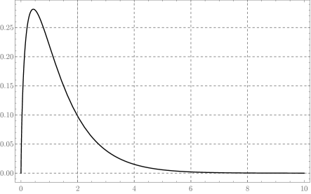
Figure 2: The function $xE_{1}(x)$.

The resulting distribution $Y$ can now be rewritten, from (40), as

$$\Pr[Y=y]=\begin{cases}y_{0}&\text{if $y=0$,}\\ y_{0}\,{\exp(y\psi(y))(q/e)^{y}}/{y!}&\text{if $y>0$.}\end{cases}$$ (52)

We call the distribution defined by (52) the digamma distribution due to the digamma term in the exponent. Combining (41) and (51) gives us

$$D_{\mathsf{KL}}({Y_{x}}\|{Y})\leq-\log y_{0}-\lambda x\log q=-\log y_{0}-\mathds{E}[Y_{x}]\log q,$$ (53)

and thus, Theorem 1 gives the upper bound

$${\mathsf{Cap}}(\mathsf{Ch}_{\mu}(\mathcal{D}))\leq-\mu\log q-\log y_{0},$$ (54)

where $q$ (and accordingly, the normalizing constant $y_{0}$) must be chosen so that the mean constraint $\mathds{E}[Y]=\mu$ is satisfied (note that this choice is unique for any given $\mu>0$). Therefore, understanding the upper bound requires a characterization of the relationship between $\mu,q$, and $y_{0}$. Since the probability mass function defining $Y$ exhibits an exponential decay, the values $\mu$ and $y_{0}$, as a function of $q$, can be numerically computed efficiently to any desired accuracy. Plots of these functions, for both distributions (43) and (52), are depicted in Figure 3. Moreover, their numerical estimates are listed, for various choices of $q\in(0,1)$, in Table B.5.

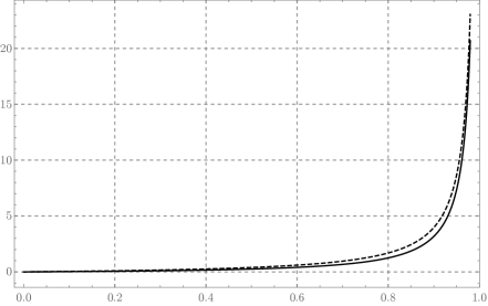
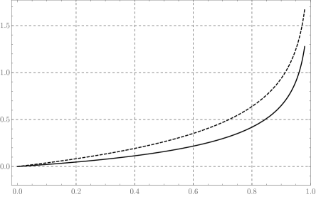
Figure 3: Plots of $\mu=\mathds{E}[Y]$ (left) and $\log(1/y_{0})$ (right), for the distribution of $Y$ in (43) (dashed) and the digamma distribution (52) (solid), as functions of $q$.

We summarize the result of this section in the following:

Theorem 10.

Let $q\in(0,1)$ be a given parameter and $Y$ be a random variable distributed according to the digamma distribution (52), for an appropriate normalizing constant $y_{0}$. Let $\mu:=\mathds{E}[Y]$, and $\mathcal{D}$ denote any Poisson distribution with positive mean. Then, capacity of the mean-limited Poisson channel $\mathsf{Ch}_{\mu}(\mathcal{D})$ satisfies

$${\mathsf{Cap}}(\mathsf{Ch}_{\mu}(\mathcal{D}))\leq-\mu\log q-\log y_{0}.$$ (55)

Figure 4 depicts the capacity upper bounds attained by the above result, as well as a similar result when the dual-feasible distribution for $Y$ is defined by (43).

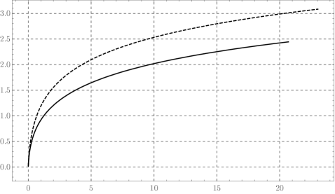
Figure 4: Capacity upper bounds (measured in bits) of Theorems 10 and 13 for the mean-limited Poisson channel in terms of $\mu=\mathds{E}[Y]$. The solid plot is the upper bound given by (55) (when the digamma distribution (52) is used for $Y$). The dashed plot is given by (64) (when (43) is used for $Y$). The first inequality in (64) and its analytic upper bound estimate would completely overlap and be indistinguishable in this plot. Likewise, the upper bound estimates of Corollary 16 for the digamma distribution (52) would result in essentially the same plot as the exact one above.

5.2 The truncation effect of replacing logarithm with harmonic numbers

The aim of this section is to provide an intuitive explanation of why the choice of the digamma distribution (52) for the distribution of $Y$, that essentially replaces the logarithmic term $\log y$ in the exponent of $\exp(y\log y)$ in (43) with harmonic numbers (equivalently, $\psi(y)$), results in improved capacity upper bounds.

For any analytic choice of $g(y)$ in (42), we can write down the Taylor series expansion of $g$ around $\mu$ as

$$g(y)=g(\mu)+(y-\mu)g^{\prime}(\mu)+\frac{1}{2}(y-\mu)^{2}g^{\prime\prime}(\mu)+\sum_{j=3}^{\infty}(y-\mu)^{j}\frac{g^{(j)}(\mu)}{j!}.$$

Let $Y_{x}$ be Poisson-distributed with mean $\lambda x$. Assuming that the above series converges, we may take the expectation of the above and, and noting that the variance of $Y_{x}$ is equal to $\lambda x$, and letting $\mu:=\lambda x$, write

$$\mathds{E}[g(Y_{x})]=g(\lambda x)+\frac{1}{2}\lambda xg^{\prime\prime}(\lambda x)+\sum_{j=3}^{\infty}\mu_{j}\frac{g^{(j)}(\lambda x)}{j!},$$

where $\mu_{j}:=\mathds{E}[(Y_{x}-\mu)^{j}]$. Now, with $g(y)=y\log y$ as in (43), we would have $g^{\prime\prime}(\lambda x)=1/(\lambda x)$, and for $j\geq 3$, $g^{(j)}(\lambda x)=O(1/x^{j-1})$ so that, for large $x$, we have the asymptotic behavior

$$\mathds{E}[g(Y_{x})]=g(\lambda x)+\frac{1}{2}+o(1).$$

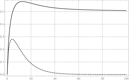
Figure 5: Plot of the KKT gap to equality in (42), as a function of $x$, attained by the distribution (43) (solid) and the digamma distribution (52) (dashed) for deletion probability $d=0.9$ (the plots would simply be scaled in $x$ for other deletion parameters). By Corollary 9, the second plot coincides with the function $\lambda xE_{1}(\lambda x)$, where $\lambda=-\log d$.

Therefore, while $g(y)$ satisfies (42) with $a=b=0$ for all $x$ (and with equality for $x=0$), the inequality exhibits an asymptotic constant gap of $1/2$ for large $x$ (see Figure 5 for a depiction). As we saw in Section 5.1, specifically (51), this gap is eliminated by choosing $g(y)$ according to (45). While this fact is verified in (51), it is worthwhile to provide a systematic way of deriving a choice of $g$ that exhibits no asymptotic gap. In order to do so, recall that the “ultimate goal” in satisfying the KKT conditions of Theorem 1 would be to exhibit a function $g(y)$ for which (51) is satisfied with equality for all $x\geq 0$. In general, this may be impossible to achieve with a choice of $g$ that does not grow faster than $y\log y+O(y)$ (so that the resulting expression (40) can be normalized to a valid probability distribution). Nevertheless, we present a “truncation technique” that obtains an approximate guarantee, in the sense that the gap in (42) exponentially decays as $x$ grows, while maintaining a controllable choice for $g$.

Assuming that (42) holds with equality and $a=b=0$, we must have $\mathds{E}[g(Y_{x})]=\mu\log\mu$, where $\mu:=\lambda x$. The right hand side, using the integral expression

$$\log\mu=\int_{0}^{\infty}\frac{e^{-t}-e^{-\mu t}}{t}\,dt,$$

and the Taylor expansion of the exponential function, can be written as

$$\mu\log\mu =\int_{0}^{\infty}\left(\frac{\mu e^{-t}}{t}+\sum_{j=1}^{\infty}\frac{\mu^{j}(-t)^{j-2}}{(j-1)!}\right)dt$$ (56)

$$=\int_{0}^{1}\left(\frac{\mu e^{-t}}{t}+\sum_{j=1}^{\infty}\frac{\mu^{j}(-t)^{j-2}}{(j-1)!}\right)dt+\mu\int_{1}^{\infty}\frac{e^{-t}-e^{-\mu t}}{t}\,dt$$

$$=\int_{0}^{1}\left(\frac{\mu e^{-t}}{t}+\sum_{j=1}^{\infty}\frac{\mu^{j}(-t)^{j-2}}{(j-1)!}\right)dt+\mu E_{1}(1)-\mu E_{1}(\mu),$$ (57)

where $E_{1}(\cdot)$ denotes the exponential integral function (49), and $E_{1}(1)\approx 0.219384$. Using (56), and noting that the factorial moments of the Poisson distribution are given by $\mathds{E}\left[\binom{Y_{x}}{j}\right]=\mu^{j}/j!$, the following function

$$\tilde{g}(y):=\int_{0}^{\infty}\left(\frac{ye^{-t}}{t}+\sum_{j=1}^{\infty}j\binom{y}{j}(-t)^{j-2}\right)dt=y\int_{0}^{\infty}\left(\frac{e^{-t}-1}{t}+\sum_{j=1}^{\infty}\binom{y-1}{j}(-t)^{j-1}\right)dt,$$ (58)

interpreted formally, is the unique solution to the functional equation

$$(\forall x\geq 0)\ \mathds{E}[\tilde{g}(y)]=\mu\log u.$$ (59)

However, the above integral definition of $\tilde{g}(y)$ does not converge (recall that $\int_{0}^{\infty}e^{-t}dt/t$ is divergent and that the inner summation in (58) only has a finite number of terms for any integer $y>0$). To address this issue, we write down a function whose expectation sharply approximates the desired value (57) for large $\mu$. In order to do so, it suffices to note that the term $\mu E_{1}(\mu)$ in (57) is exponentially small in $\mu$ and can thus be ignored in the approximation. Now, consider a truncated variation of $\tilde{g}$ defined, by simply truncating the upper limit of the integration at $t=1$, as

$$\hat{g}(y) :=y\int_{0}^{1}\left(\frac{e^{-t}-1}{t}+\sum_{j=1}^{\infty}\binom{y-1}{j}(-t)^{j-1}\right)dt$$

$$=y(-\gamma-E_{1}(1))+y\int_{0}^{1}\sum_{j=1}^{\infty}\binom{y-1}{j}(-t)^{j-1}dt$$

$$=y(-\gamma-E_{1}(1))-y\sum_{j=1}^{\infty}\binom{y-1}{j}\frac{(-1)^{j}}{j}$$

$$=-yE_{1}(1)+y\psi(y),$$

where, in the above, $\gamma$ is the Euler-Mascheroni constant, $\psi(y)$ is the digamma function (with $y\psi(y)$ to be understood as zero for $y=0$), and we have used the Newton series expansion of the digamma function

$$\psi(y+1)=-\gamma-\sum_{j=1}^{\infty}\frac{(-1)^{j}}{j}\binom{y}{j}.$$ (60)

From (57), we see that

$$\mathds{E}[\hat{g}(Y_{x})]=\mu\log\mu-\mu E_{1}(1)+\mu E_{1}(\mu),$$ (61)

so that the function $\hat{g}(y)+yE_{1}(1)$ provides the desired approximation. This is precisely the function $g$ that we defined in (45).

Remark 11.

We could have truncated the integral upper limit to any constant $c\in[0,1]$ and yet obtain an exponentially sharp approximation of $\mu\log\mu$ for large $\mu$ (choosing $c>1$, though, would result in an exponential growth of $\hat{g}(y)$ in $y$ and, subsequently, an expression for the probability mass function of $Y$ that cannot be normalized to a valid distribution). Among these choices, truncation at $c=1$ provides the closest possible approximation.

Remark 12.

The observation that the expression for $\tilde{g}(y)$, the solution to the functional equation (59), does not converge shows that the KKT equality conditions (25) of Theorem 1 cannot be simultaneously satisfied for all $x\geq 0$. In other words, for any mean-limited Poisson channel, there is no input distribution $X$ with full support on non-negative integers that achieves the capacity of the channel. However, the optimal $X$ must have infinite support (since otherwise, for large enough $x$, the KL divergence on the left hand side of (24) becomes infinite and the KKT conditions would be violated). The claim that the optimal $X$ cannot have full support makes intuitive sense. Intuitively, if the input distribution has nonzero support on some $x>0$, then the corresponding channel output is expected to be $\lambda x$ with a variance of $\lambda x$. Therefore, any input $x^{\prime}$ for which $\lambda|x-x^{\prime}|$ is too close to the standard deviation $\sqrt{\lambda x}$ would cause confusion at the decoder and should be avoided. Roughly, this means that if $x$ is on the support of the transmitter’s input distribution $X$, the next symbol in the codebook should be picked at $x+\Omega(\sqrt{x/\lambda})$.

5.3 Analytic estimates

It is desirable to provide sharp upper and lower bound estimates on the mean and normalizing constants of the distribution (43) and the digamma distribution (52) in terms of elementary or standard special functions, and that is what we achieve in this section.

5.3.1 Estimates by standard special functions

First, we obtain sharp estimates on the parameters of the distribution (43) in terms of standard special functions. Since the refined digamma distribution (52) achieves better capacity upper bounds than (43), and, as we see in the next section, we are able to estimate the parameters of the former sharply in terms of elementary functions, the result of this section should be regarded as a side result. However, the techniques presented here will be used for the more complex problem of approximating the inverse binomial distribution, for the deletion channel problem, in terms of standard special functions. It is thus natural to demonstrate the approximation techniques for the mean-limited Poisson channel first before approaching the slightly more complex case of the binomial channel.

We recall the standard special function Lerch transcendent (cf. [ref:EMOT53, p. 27]), given by

$$\Phi(z,s,\alpha):=\sum_{k=0}^{\infty}{\frac{z^{k}}{(k+\alpha)^{s}}}={\frac{1}{\Gamma(s)}}\int_{0}^{\infty}{\frac{t^{{s-1}}e^{{-\alpha t}}}{1-ze^{{-t}}}}\,dt.$$ (62)

The approximation of (43) in terms of the above function is given by the following theorem, that we prove in Appendix A:

Theorem 13.

Let $q\in(0,1)$ be a given parameter and $Y$ be a random variable distributed according to (43), for an appropriate normalizing constant $y_{0}$. Let $\mu:=\mathds{E}[Y]$, and consider constants $\underline{\sigma}:=1/6$ and $\overline{\sigma}:=0.177\approx 16/90$. Define special functions $S_{0}(q,\sigma):=\Phi(q,1/2,1+\sigma)$ and $S_{1}(q,\sigma):=\frac{q}{\sqrt{2\pi}}\Phi(q,-1/2,1+\sigma)-\sigma S_{0}(q,\sigma)$. Then,

1. We have the bounds

   $$y_{0} \geq 1/(1+S_{0}(q,\underline{\sigma}))=:\underline{y_{0}}, y_{0} \leq 1/(1+S_{0}(q,\overline{\sigma}))=:\overline{y_{0}},$$ (63)

   $$\mu \geq S_{1}(q,\overline{\sigma})/(1+S_{0}(q,\underline{\sigma}))=:\underline{\mu}, \mu \leq S_{1}(q,\underline{\sigma})/(1+S_{0}(q,\overline{\sigma}))=:\overline{\mu}.$$

2. Let $\mathcal{D}$ denote any Poisson distribution with positive mean. Then, capacity of the mean-limited Poisson channel $\mathsf{Ch}_{\mu}(\mathcal{D})$ satisfies

   $${\mathsf{Cap}}(\mathsf{Ch}_{\mu}(\mathcal{D}))\leq-\mu\log q-\log y_{0}\leq-\overline{\mu}\log q-\log\underline{y_{0}}.$$ (64)

∎

As demonstrated in Figure 6, the expressions in (63) provide remarkably sharp upper and lower bound estimates on the normalizing constant $y_{0}$ and the expectation $\mu$, which are accurate within a multiplicative factor of about $1\pm 0.004$ for all $q\in(0,1)$.

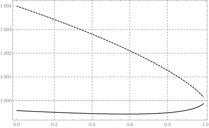
Figure 6: Quality of the approximations in (63) as a function of $q$. Left: $\overline{\mu}/\mu$ (solid) and $\underline{\mu}/\mu$ (dashed). Right: $(\log\overline{y_{0}})/(\log y_{0})$ (solid) and $(\log\underline{y_{0}})/(\log y_{0})$ (dashed).

5.3.2 Estimate by the negative binomial distribution

In Section 5.3.1, we obtained sharp estimates on the mean and the normalizing constant of the distribution $Y$ in (43) in terms of standard special functions. In this section, we provide similar estimates, albeit not as sharp, for the distribution (43) in terms of elementary functions.

Recall that a negative binomial distribution of order $r$ with “success probability” $q\in(0,1)$ is defined by the probability mass function

$$\mathsf{NegBin}_{r,q}(y)=\binom{y+r-1}{y}(1-q)^{r}q^{y},\quad y=0,1,\ldots,$$ (65)

and has mean $\mu=qr/(1-q)$ [ref:DS12, Section 5.3]. The asymptotic behavior of (65) at large $y$ can be understood by the Stirling approximation $\Gamma(1+y)\sim\sqrt{2\pi y}(y/e)^{y}$; namely,

$$\mathsf{NegBin}_{r,q}(y) =\frac{\Gamma(y+r)(1-q)^{r}q^{y}}{\Gamma(y+1)\Gamma(r)}$$

$$\sim\frac{(1-q)^{r}q^{y}}{\Gamma(r)}\sqrt{\frac{y+r}{y+1}}e^{1-r}\frac{(y+r-1)^{y+r-1}}{y^{y}}$$

$$\sim\frac{(1-q)^{r}}{\Gamma(r)}e^{1-r}\left(1+\frac{r-1}{y}\right)^{y}q^{y}y^{r-1}$$

$$\sim\frac{(1-q)^{r}}{\Gamma(r)}\,q^{y}y^{r-1}$$ (66)

Throughout this section, we focus on the special case $r=1/2$, so (66) becomes

$$\mathsf{NegBin}_{r,q}(y)\sim\sqrt{\frac{1-q}{\pi}}\,\frac{q^{y}}{\sqrt{y}}.$$ (67)

We prove the following key estimate on the binomial coefficient $\binom{y-1/2}{y}$ that is used to provide accurate estimates on the parameters of the inverse binomial distribution:

Lemma 14.

Let ${\underline{\gamma}}:={2}/{e^{1+\gamma}}\approx 0.413099$ and ${\overline{\gamma}}:=1/\sqrt{2e}\approx 0.428882$, where $\gamma\approx 0.57721$ is the Euler-Mascheroni constant. Then, for all $y\geq 1$,

$$\binom{y-1/2}{y}\,{\underline{\gamma}}\leq\frac{\exp(y\psi(y)-y)}{y!}\leq\binom{y-1/2}{y}\,{\overline{\gamma}}.$$

Proof.

Consider the ratio

$$g(y)=\frac{\binom{y-1/2}{y}}{\exp(y\psi(y))/(y!e^{y})}=\frac{\Gamma(y+1/2)}{\Gamma(1/2)\exp(y\psi(y)-y)}=\frac{1}{\sqrt{\pi}}\Gamma(y+1/2)\exp(y-y\psi(y)),$$ (68)

We use the following claim (see Appendix B.1):

Claim 15.

The function $g(y)$ defined in (68) is a decreasing function of $y>0$.

The above claim implies that, for all $y\geq 1$, we must have

$$g(1)\geq g(y)\geq\lim_{y\to\infty}g(y),$$

assuming that the limit exists (that we will show next). We have

$$g(0)=\frac{1}{\sqrt{\pi}}\Gamma(3/2)\exp(1-\psi(1))=\frac{e^{1+\gamma}}{2}\approx 2.420728.$$

Recall, from (46), that

$$\exp(y\psi(y))/(y!e^{y})\sim\frac{1}{\sqrt{2\pi ey}},$$

and similarly, from (67), that

$$\binom{y-1/2}{y}\sim{\frac{1}{\sqrt{\pi y}}},$$

and therefore,

$$\lim_{y\to\infty}g(y)=\sqrt{2e}\approx 2.331643.$$

The result follows. ∎

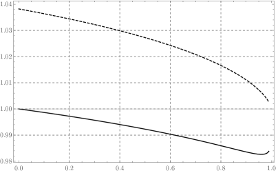
Figure 7: Quality of the approximations by Corollary 16 as a function of $q$. Left: $\overline{\mu}/\mu$ (solid) and $\underline{\mu}/\mu$ (dashed). Right: $(\log\overline{y_{0}})/(\log y_{0})$ (solid) and $(\log\underline{y_{0}})/(\log y_{0})$ (dashed). The notation $\overline{\mu}$ and $\underline{\mu}$ ($\overline{y_{0}}$ and $\underline{y_{0}}$) respectively refer to the upper and lower bound estimates on $\mu$ ($y_{0}$) by Corollary 16.

Using the above approximations, we are able to prove the following lower and upper bound estimates on the parameters of the digamma distribution (52) in terms of elementary functions (see Figure 7 for a depiction of the quality of the approximations).

Corollary 16.

Let ${\underline{\gamma}}$ and ${\overline{\gamma}}$ be as in Lemma 14, and $Y$ be distributed according to the digamma distribution (52). Then,

1. For all $y\geq 1$,

   $${\underline{\gamma}}\,\mathsf{NegBin}_{1/2,q}(y)\leq\sqrt{1-q}\Pr[Y=y]/y_{0}\leq{\overline{\gamma}}\,\mathsf{NegBin}_{1/2,q}(y).$$ (69)

2. The normalizing constant $y_{0}$ satisfies

   $$\log\left(1+{\underline{\gamma}}\left(\frac{1}{\sqrt{1-q}}-1\right)\right)\leq-\log y_{0}\leq\log\left(1+{\overline{\gamma}}\left(\frac{1}{\sqrt{1-q}}-1\right)\right).$$ (70)

3. The mean $\mu=\mathds{E}[Y]$ satisfies

   $$\frac{{\underline{\gamma}}q}{2(1-q)^{3/2}}\leq\frac{\mu}{y_{0}}\leq\frac{{\overline{\gamma}}q}{2(1-q)^{3/2}},$$ (71)

   and,

   $$\frac{{\underline{\gamma}}q}{2(1-q)(\sqrt{1-q}+{\overline{\gamma}}(1-\sqrt{1-q}))}\leq\mu\leq\frac{{\overline{\gamma}}q}{2(1-q)(\sqrt{1-q}+{\underline{\gamma}}(1-\sqrt{1-q}))}.$$ (72)

Proof.

The first part is immediate from the expression of the digamma distribution (52) combined with the result of Lemma 14. Now, let $Z$ be distributed according to $\mathsf{NegBin}_{1/2,q}$, and write, from the definition of the normalizing constant,

$$1/y_{0} ={1+\sum_{y=1}^{\infty}\Pr[Y=y]/y_{0}}$$

$$\stackrel{{\scriptstyle\eqref{eqn:Poi:PYnegbin}}}{{\leq}}{1+\left(\frac{{\overline{\gamma}}}{\sqrt{1-q}}\right)\sum_{z=1}^{\infty}\Pr[Z=z]}$$

$$={1+\left(\frac{{\overline{\gamma}}}{\sqrt{1-q}}\right)\left(1-\sqrt{1-q}\right)}$$

$$=1+{\overline{\gamma}}\left(\frac{1}{\sqrt{1-q}}-1\right),$$ (73)

which, after taking the logarithms of both sides, proves the upper bound in (70). Proof of the lower bound is similar. To upper bound the mean, we may write

$$\frac{\mu}{y_{0}} =\sum_{y=1}^{\infty}y\Pr[Y=y]/y_{0}$$

$$\stackrel{{\scriptstyle\eqref{eqn:Poi:PYnegbin}}}{{\leq}}\sum_{z=1}^{\infty}{\overline{\gamma}}z\Pr[Z=z]/\sqrt{1-q}$$

$$={\overline{\gamma}}\mathds{E}[Z]/\sqrt{1-q}=\frac{{\overline{\gamma}}q}{2(1-q)^{3/2}},$$ (74)

which, combined with a similar lower bound, proves (72). Finally, combining this result with (70) yields (72). ∎

5.4 Derivation of the capacity upper bound for the Poisson-repeat channel

In order to obtain a capacity upper bound for the Poisson-repeat channel, it suffices to combine Corollary 5 with either Theorem 10 or Theorem 13. Let $\mathsf{Ch}$ be a $\mathcal{D}$-repeat channel, where $\mathcal{D}$ is a Poisson distribution with mean $\lambda$. The probability $d$ assigned by $\mathcal{D}$ to zero is thus equal to $e^{-\lambda}$, and its complement is $p:=1-d=1-e^{-\lambda}$. Since $d$ captures the “deletion probability” of the channel, we parameterize the channel in terms of $p$ rather than the Poisson parameter $\lambda$. Note that $\lambda=-\log(1-p)$. From (29), we may write

$${\mathsf{Cap}}(\mathsf{Ch}) \leq\sup_{\mu>0}\frac{{\mathsf{Cap}}(\mathsf{Ch}_{\mu}(\mathcal{D}))}{-\mu/\log(1-p)+1/p}.$$

We may now use Theorem 10 with the corresponding choice for the random variable $Y$ with parameter $q$, mean $\mu$ and normalizing constant $y_{0}$ and write, using (55),

$${\mathsf{Cap}}(\mathsf{Ch}) \leq\sup_{q\in(0,1)}\frac{-\mu\log q-\log y_{0}}{-\mu/\log(1-p)+1/p}.$$ (75)

Of course, this result would remain valid had we used Theorem 13 and (43) for the distribution of $Y$. Furthermore, the analytic approximations of Corollary 16 may be used to upper bound the right hand side of (75) by the supremum of an elementary function of the channel parameter and $q$ (which can be shown to be concave in $q$). We summarize the above result in the following theorem:

Theorem 17.

Let $\mathsf{Ch}$ be a Poisson-repeat channel with deletion probability $d\in(0,1)$ (or equivalently, repetition mean $\lambda=\log(1/d)$ per bit). For a parameter $q\in(0,1)$, let $Y$ be distributed according to either the distribution (43) or the digamma distribution (52) with an appropriate normalizing constant $y_{0}$ and let $\mu:=\mathds{E}[Y]$ denote its mean. Then,

$${\mathsf{Cap}}(\mathsf{Ch}) \leq\sup_{q\in(0,1)}\frac{-\mu\log q-\log y_{0}}{-\mu/\log d+1/(1-d)}.$$ (76)

Furthermore, let ${\underline{\gamma}}:={2}/{e^{1+\gamma}}\approx 0.413099$ and ${\overline{\gamma}}:=1/\sqrt{2e}\approx 0.428882$, where $\gamma\approx 0.57721$ is the Euler-Mascheroni constant. Then,

$${\mathsf{Cap}}(\mathsf{Ch}) \leq\sup_{q\in(0,1)}\frac{-\overline{\mu}\log q-\log\underline{y_{0}}}{-\underline{\mu}/\log d+1/(1-d)},$$ (77)

where

$$\overline{\mu} :=\frac{{\overline{\gamma}}q}{2(1-q)(\sqrt{1-q}+{\underline{\gamma}}(1-\sqrt{1-q}))},$$ (78)

$$\underline{\mu} :=\frac{{\underline{\gamma}}q}{2(1-q)(\sqrt{1-q}+{\overline{\gamma}}(1-\sqrt{1-q}))},$$

$$\underline{y_{0}} :=1+{\overline{\gamma}}\left(\frac{1}{\sqrt{1-q}}-1\right).$$

∎

Remark 18.

Observe that the distributions of $Y$ defined by (43) or the digamma distribution (52) in Theorem 17 only depend on the choice of the parameter $q$ and not the channel parameter $d$ at all. Therefore, the calculations of mean and normalizing constant for various choices of $q$ can be reused for the computation of the capacity upper bound for different choices of $d$.

Observe that, as $p\rightarrow 0$, the right hand side of (75) converges to

$$p\sup_{q\in(0,1)}\frac{-\mu\log q-\log y_{0}}{\mu+1},$$ (79)

and that the expression under the supremum is independent of the channel parameter $p$. The expression under the supremum is plotted in Figure 8 and can be numerically calculated efficiently, which results in the following corollary:

Corollary 19.

Let ${\mathscr{C}}(d)$ denote the capacity of the Poisson-repeat channel with deletion probability $d$. Then for $d\to 1$,

$${\mathscr{C}}(d)\leq 0.464421(1-d)\cdot(1+o(1))\ \text{\rm bits per channel use}.$$

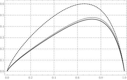
Figure 8: The expression inside the supremum in (79) (measured in bits) plotted as a function of $q$ and with respect to the choices (52) (solid) and (43) (dashed) for the distribution of $Y$. The maximums are attained at $q\approx 0.724762$ (solid) and $q\approx 0.659046$ (dashed), resulting in supremums $\approx 0.464420$ (solid) and $\approx 0.601549$ (dashed). The analytic estimates of Theorem 13 result in an indistinguishable plot from the dashed one, and a slightly higher supremum of $\approx 0.602987$ attained at $q\approx 0.658810$. The dotted plot depicts the elementary upper bound resulting from (78), where the maximum is $\approx 0.479454$ and attained at $q\approx 0.727855$.

Plots of the resulting capacity upper bounds for general $d$ are given in Figure 9. Moreover, the corresponding numerical values for the plotted curves are listed, for various choices of the deletion parameter $d$, in Table B.5.

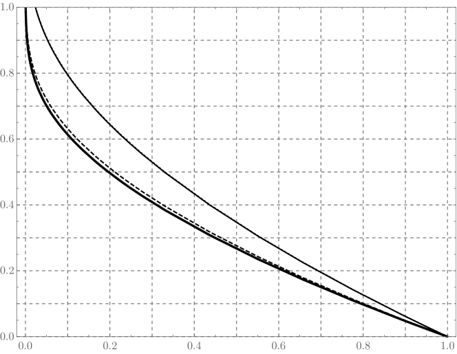
Figure 9: Upper bounds (in bits per channel use) on the capacity of the Poisson-repeat channel given by Theorem 17, plotted as a function of the deletion probability $d=1-p=e^{-\lambda}$. The bounds are obtained using i) The digamma distribution (52) for $Y$ (solid, thick), ii) The distribution (43) for $Y$ (solid), iii) The elementary upper bound estimates of (78) on the parameters of the digamma distribution (52) (dashed), iv) The analytic upper bound estimates of Theorem 13 on the parameters of (43) (dotted, nearly indistinguishable from the solid curve obtained by a numerical computation of the actual parameters of the distribution).

 

6 Upper bounds on the capacity of the deletion channel

6.1 The inverse binomial distribution

Let $\mathsf{InvBin}_{p,q}$ be a distribution on non-negative integers, parameterized by $p\in(0,1]$ and $q\in(0,1)$, and defined by the probability mass function

$$\mathsf{InvBin}_{p,q}(y):=y_{0}\binom{y/p}{y}q^{y}\exp(-yh(p)/p),$$ (80)

where $h(p)$ is the binary entropy function, and $y_{0}\in(0,1)$ is the appropriate normalizing constant:

$$1/y_{0}=1+\sum_{y=0}^{\infty}\binom{y/p}{y}q^{y}\exp(-yh(p)/p).$$

Note that, when $p=1$, the above reduces to a geometric distribution.

By the Stirling approximation, we may write the well known asymptotic expression

$$\binom{x}{px} \sim\frac{(x/e)^{x}}{\sqrt{2\pi p(1-p)x}(px/e)^{px}(x(1-p)/e)^{(1-p)x}}$$

$$=\frac{\exp(h(p)x)}{\sqrt{2\pi p(1-p)x}},$$

and thus, we can identify the asymptotic behavior of (80) at $y\rightarrow\infty$ as

$$\mathsf{InvBin}_{p,q}(y) \sim y_{0}\frac{q^{y}}{\sqrt{2\pi(1-p)y}},$$ (81)

implying that the normalizing constant is well defined, leading to a legitimate distribution, exactly when $q\in(0,1)$. Moreover, the expectation of the distribution can be made arbitrarily small as $q\to 0$ and arbitrarily large as $q\to 1$ (since, by (81), when $q=1$ we have $\mathsf{InvBin}_{p,1}(y)/y_{0}=\Theta(1/\sqrt{y})$ and the summation defining $y_{0}$ becomes divergent). Therefore, by varying the value of $q\in(0,1)$, it is possible to adjust the expectation of the distribution to any desired positive value.

6.1.1 Estimate by the negative binomial distribution

As was the case for the distribution (40) related to the Poisson-repeat channel, in this section we show that the inverse binomial distribution can be approximated by a negative binomial distribution of order $r=1/2$. Towards this goal, we will use the following analytic claim (derived in Appendix B.2):

Claim 20.

Let $p\in(0,1)$. The ratio

$$\rho(y):=\frac{\binom{y/p}{y}\exp(-yh(p)/p)}{\binom{y-1/2}{y}}$$ (82)

is a decreasing function of $y>0$ for $p<1/2$, is equal to $1$ for $p=1/2$, and is an increasing function of $y>0$ for $p>1/2$.

The fact that, by Claim 20, $\rho(y)=1$ for $p=1/2$ implies that the inverse binomial distribution for the special case $p=1/2$ is precisely a negative binomial distribution, and thus in this case, we have

$$y_{0}=\sqrt{1-q},\quad\mathds{E}[\mathsf{InvBin}_{1/2,q}]=q/(2(1-q)).$$ (83)

We show that, when $p\neq 1/2$, the inverse binomial distribution is still reasonably approximated by a negative binomial distribution of order $r=1/2$, and that the quality of this approximation improves as $p$ gets closer to $1/2$. Define

$$\beta_{0}:=\rho(1)=(2/p)\exp(-h(p)/p).$$ (84)

By combining (67) and (81), the ratio in (82) satisfies

$$\beta_{1}:=\lim_{y\to\infty}\rho(y)=\frac{1}{\sqrt{2(1-p)}}.$$ (85)

We observe that, when $p=1/2$, we have $\beta_{0}=\beta_{1}=1$, and $\beta_{0}\to 2/e\approx 0.735759$ as $p\to 0$. For $p<1/2$, we have $\beta_{0}>\beta_{1}$, whereas for $p>1/2$, we have $\beta_{0}<\beta_{1}$. This leads to the following analogous result to (69):

Lemma 21.

For a parameter $p\in(0,1)$, let the $\beta_{0}$ and $\beta_{1}$ be the constants defined in (84) and (85). Let $\underline{\beta}:=\min\{\beta_{0},\beta_{1}\}$ and $\overline{\beta}:=\max\{\beta_{0},\beta_{1}\}$ (in particular, for $p=1/2$, we have $\underline{\beta}=\overline{\beta}=1$). Then, for all $y\geq 1$,

$$\underline{\beta}\,\mathsf{NegBin}_{1/2,q}(y)\leq\frac{\sqrt{1-q}}{y_{0}}\,\mathsf{InvBin}_{p,q}(y)\leq\overline{\beta}\,\mathsf{NegBin}_{1/2,q}(y).$$ (86)

The above lemma can now be used to derive upper and lower estimates on the mean and normalizing constant of an inverse binomial distribution. Let $Y$ be distributed according to $\mathsf{InvBin}_{p,q}$, and $y_{0}$ denote the corresponding normalizing constant in (80). Furthermore, let a random variable $Z$ be distributed according to $\mathsf{NegBin}_{1/2,q}$. As in (73), we may now proceed by writing

$$1/y_{0} =1+\sum_{y=1}^{\infty}\Pr[Y=y]/y_{0}$$

$$\stackrel{{\scriptstyle\eqref{eqn:invbin:estimate}}}{{\leq}}1+\frac{\overline{\beta}}{\sqrt{1-q}}\,\sum_{z=1}^{\infty}\Pr[Z=z]$$

$$=1+\frac{\overline{\beta}}{\sqrt{1-q}}\left(1-\sqrt{1-q}\right)$$

$$=1+\overline{\beta}\left(\frac{1}{\sqrt{1-q}}-1\right).$$

Moreover, we may derive a similar expression to (74), namely, letting $\mu:=\mathds{E}[Y]$, that we have

$$\frac{\mu}{y_{0}}\leq\frac{\overline{\beta}q}{2(1-q)^{3/2}}.$$ (87)

Similarly, we may derive lower bounds on $\mu$ and $y_{0}$ by using the lower bounding constant $\underline{\beta}$. This leads to the following result, which is analogous to Corollary 16 (see Figure 10 for plots on the quality of this approximation):

Corollary 22.

Consider the inverse binomial distribution $\mathsf{InvBin}_{p,q}$, with mean $\mu$, as defined in (80). Define $\underline{\beta}$ (resp., $\overline{\beta}$) to be the minimum (resp., the maximum) of the two constants $(2/p)\exp(-h(p)/p)$ and ${1}/{\sqrt{2(1-p)}}$. Then,

$$\log\left(1+\underline{\beta}\left(\frac{1}{\sqrt{1-q}}-1\right)\right)\leq-\log y_{0}\leq\log\left(1+\overline{\beta}\left(\frac{1}{\sqrt{1-q}}-1\right)\right),$$ (88)

$$\frac{\underline{\beta}q}{2(1-q)^{3/2}}\leq\frac{\mu}{y_{0}}\leq\frac{\overline{\beta}q}{2(1-q)^{3/2}},$$ (89)

$$\frac{\underline{\beta}q}{2(1-q)(\sqrt{1-q}+\overline{\beta}(1-\sqrt{1-q}))}\leq\mu\leq\frac{\overline{\beta}q}{2(1-q)(\sqrt{1-q}+\underline{\beta}(1-\sqrt{1-q}))}.$$ (90)

6.1.2 Estimates by standard special functions

The estimates of Corollary 22 provide high-quality upper and lower bounds on the mean and the normalizing constant of an inverse binomial distribution in terms of elementary functions. In fact, the bounds are exact for $p=1/2$, and a numerical computation shows that (88) and (90) are within a multiplicative factor of about $1.2$ for all $p\leq 0.8$ and $q\in(0,1)$. However, as $p$ approaches $1$, the quality of the estimates degrade, as the ratio between $\overline{\beta}$ and $\underline{\beta}$ tends to infinity when $p\to 1$. In this section, we provide a different set of upper and lower bounds in terms of standard special functions.

Our starting point is the following claim on the binomial coefficients (see Appendix B.3 for a derivation):

Claim 23.

There are universal constants $\underline{\alpha},\overline{\alpha}>0$ such that for all $y\geq 1$ and $p\in(0,1)$, we have

$$\frac{\exp(yh(p)/p)}{\sqrt{2\pi((1-p)y+\underline{\alpha})}}\leq\binom{y/p}{y}\leq\frac{\exp(yh(p)/p)}{\sqrt{2\pi((1-p)y+\overline{\alpha})}}.$$ (91)

In particular, one may take $\underline{\alpha}=0.19$ and $\overline{\alpha}=0.12$.

Now, given a random variable $Y$ that is distributed according to (80), we can write

$$1/y_{0} =1+\sum_{y=1}^{\infty}\binom{y/p}{y}q^{y}\exp(-yh(p)/p)$$

$$\stackrel{{\scriptstyle\eqref{eqn:claim:binomial}}}{{\leq}}1+\sum_{y=1}^{\infty}\frac{q^{y}}{\sqrt{2\pi((1-p)y+\overline{\alpha})}}$$

$$=1+\frac{1}{\sqrt{2\pi(1-p)}}\sum_{y=1}^{\infty}\frac{q^{y}}{\sqrt{y+\overline{\alpha}/(1-p)}}$$

$$=1+\frac{q\,\Phi(q,1/2,1+\overline{\alpha}/(1-p))}{\sqrt{2\pi(1-p)}},$$

where $\Phi(\cdot)$ denotes the Lerch transcendent (62). Similarly, an upper bound on $y_{0}$ may be obtained by replacing $\overline{\alpha}$ with $\underline{\alpha}$ in the above. We now upper bound the mean $\mu=\mathds{E}[Y]$ as follows:

$$\mu/y_{0} =\sum_{y=1}^{\infty}\binom{y/p}{y}yq^{y}\exp(-yh(p)/p)$$

$$\stackrel{{\scriptstyle\eqref{eqn:claim:binomial}}}{{\leq}}\sum_{y=1}^{\infty}\frac{yq^{y}}{\sqrt{2\pi((1-p)y+\overline{\alpha})}}$$

$$=\frac{1}{\sqrt{2\pi(1-p)}}\sum_{y=1}^{\infty}\frac{yq^{y}}{\sqrt{y+\overline{\alpha}/(1-p)}}$$

$$=\frac{1}{\sqrt{2\pi(1-p)}}\left(\sum_{y=1}^{\infty}q^{y}\sqrt{y+\overline{\alpha}/(1-p)}-\frac{\overline{\alpha}}{1-p}\sum_{y=1}^{\infty}\frac{q^{y}}{\sqrt{y+\overline{\alpha}/(1-p)}}\right)$$

$$=\frac{\Phi(q,-1/2,1+\overline{\alpha}/(1-p))}{\sqrt{2\pi(1-p)}}-\frac{\overline{\alpha}\,\Phi(q,1/2,1+\overline{\alpha}/(1-p))}{\sqrt{2\pi(1-p)^{3}}},$$

and similarly, a lower bound may be obtained by replacing $\overline{\alpha}$ with $\underline{\alpha}$. The above estimates are summarized in the following (and depicted in Figure 10):

Theorem 24.

For parameters $p,q\in(0,1)$, let $Y$ be distributed according to the inverse binomial distribution (80), for an appropriate normalizing constant $y_{0}$, and let $\mu:=\mathds{E}[Y]$. Let $\underline{\alpha}$, $\overline{\alpha}$ be the constants from Claim 23; namely, $\underline{\alpha}:=0.19$ and $\overline{\alpha}:=0.12$. Define the functions

$$S_{0}(p,q,\alpha) :=1+\frac{q\,\Phi(q,1/2,1+\alpha/(1-p))}{\sqrt{2\pi(1-p)}},$$ (92)

$$S_{1}(p,q,\alpha) :=\frac{\Phi(q,-1/2,1+\alpha/(1-p))}{\sqrt{2\pi(1-p)}}-\frac{\alpha,\Phi(q,1/2,1+\alpha/(1-p))}{\sqrt{2\pi(1-p)^{3}}},$$ (93)

where $\Phi(\cdot)$ denotes the Lerch transcendent (62). Then, the following estimates hold:

$$\begin{gathered}S_{0}(p,q,\underline{\alpha})\leq 1/y_{0}\leq S_{0}(p,q,\overline{\alpha}),\\ S_{1}(p,q,\underline{\alpha})\leq\mu/y_{0}\leq S_{1}(p,q,\overline{\alpha}),\\ S_{1}(p,q,\underline{\alpha})/S_{0}(p,q,\overline{\alpha})\leq\mu\leq S_{1}(p,q,\overline{\alpha})/S_{0}(p,q,\underline{\alpha}).\end{gathered}$$ (94)

Compared with the negative binomial estimate (Corollary 22), the above estimates are inferior around $p=1/2$. However, unlike the former, Theorem 24 provides remarkably accurate estimates on the mean and the normalizing constant of an inverse binomial distribution for all $p,q\in(0,1)$.

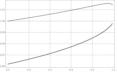
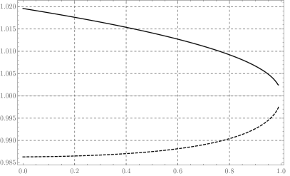
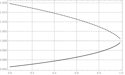
Figure 10: Quality of the approximations on the parameters of a negative binomial distribution with $p=0.1$ in terms of elementary functions (top; using Corollary 22) and standard special functions (bottom; using Theorem 24). The plots on the left depict the ratios $\overline{\mu}/\mu$ (solid) and $\underline{\mu}/\mu$ (dashed), as functions of $q$, where $\overline{\mu}$ and $\underline{\mu}$ are respectively the upper and lower bound estimates on the mean $\mu$. Similarly, the plots on the right depict the ratios $(\log\overline{y_{0}})/(\log y_{0})$ (solid) and $(\log\underline{y_{0}})/(\log y_{0})$ (dashed), as functions of $q$, where $\overline{y_{0}}$ and $\underline{y_{0}}$ are respectively the upper and lower bound estimates on the normalizing constant $y_{0}$.

6.2 Upper bounds on the capacity of a mean-limited Binomial channel

In this section, we consider the convolution channel $\mathsf{Ch}_{\mu}({\mathsf{Ber}}_{p})$, where ${\mathsf{Ber}}_{p}$ is the Bernoulli distribution with mean $p$ (and $d=1-p$ is the deletion probability). The input to this channel is a non-negative integer $X$ and the output is a sample from the binomial distribution ${\mathsf{Bin}}_{X,p}$. In particular, we have $\mathds{E}[Y]=p\mathds{E}[X]$, and thus the mean constraint implies that $\mathds{E}[X]=\mu/p$.

6.2.1 Capacity upper bound using the inverse binomial distribution

In order to upper bound the capacity of $\mathsf{Ch}_{\mu}({\mathsf{Ber}}_{p})$, we shall apply Theorem 1 with an appropriate choice for the distribution of $Y$. Recall that, for every $x\geq 0$, the distribution of $Y_{x}$ is binomial (${\mathsf{Bin}}_{x,p}$) with parameters $x$ (number of trials), $p$ (success probability), and mean $\mathds{E}[Y_{x}]=px$. That is, for all integers $y\geq 0$,

$$\Pr[Y_{x}=y]=\binom{x}{y}p^{y}(1-p)^{x-y}.$$ (95)

Intuitively, the constraints in (24) should be generally satisfied with as small a gap as possible. Indeed, according to the KKT conditions, equality must hold for every point on the support of an optimal input distribution $X$. Moreover, the optimal (and in fact, any feasible) $X$ must have infinite support, since otherwise, for large enough $x$ the KL divergence $D_{\mathsf{KL}}({Y_{x}}\|{Y})$ for the corresponding output distribution $Y$ would be infinite, violating (24). One may hope that, in the ideal case, the optimum distribution would satisfy all constraints with equality (and that would be necessary if the optimum $X$ had full support). However, in Remark 30, we rule out this possibility.

In order to identify a feasible choice for $Y$, we first use convexity to show that an inverse binomial distribution, as defined in (80), is a feasible choice. Let $Y$ be distributed according to $\mathsf{InvBin}_{p,q}$. Note that the entropy of $Y_{x}$ can be written as

$$H(Y_{x}) =xh(p)-\mathds{E}\left[\log\binom{x}{Y_{x}}\right],$$ (96)

where $h(p)$ is the binary entropy function. Then, $D_{\mathsf{KL}}({Y_{x}}\|{Y})$ can be written as

$$D_{\mathsf{KL}}({Y_{x}}\|{Y}) =\sum_{y=0}^{\infty}\Pr[Y_{x}=y]\log\frac{\Pr[Y_{x}=y]}{\Pr[Y=y]}$$

$$\stackrel{{\scriptstyle\eqref{eqn:invbin}}}{{=}}-H(Y_{x})-\log y_{0}-\mathds{E}[Y_{x}]\log q+\mathds{E}[Y_{x}]h(p)/p-\mathds{E}\left[\log\binom{Y_{x}/p}{Y_{x}}\right]$$

$$\stackrel{{\scriptstyle\eqref{eqn:del:HYx}}}{{=}}\mathds{E}\log\left[\binom{x}{Y_{x}}\Big{/}\binom{Y_{x}/p}{Y_{x}}\right]-xp\log q-\log y_{0}.$$ (97)

Let $\overline{Y_{x}}:=x-Y_{x}$, and observe that the distribution of $\overline{Y_{x}}$ is also binomial over $x$ trials, but with success probability $1-p$; i.e., ${\mathsf{Bin}}_{x,1-p}$. Define

$$f(y):=\log\left[\binom{x}{y}\Big{/}\binom{y/p}{y}\right].$$

We can now write the expectation in (97) as

$$\mathds{E}[f(Y_{x})]=\log x!-\mathds{E}[\log Y_{x}]-\mathds{E}[\log\overline{Y_{x}}]-\mathds{E}\left[\log\binom{x}{Y_{x}}\right].$$

By the Bohr-Mollerup theorem (or simply positivity of the trigamma function), $-\log\Gamma(y+1)$ is a concave function of $y$. Moreover, we observe the following, which implies that $f(y)$ is a concave function of $y$ (see Appendix B.4 for a proof):

Claim 25.

The function

$$f(y):=\log\binom{y}{py}=\log\frac{\Gamma(y+1)}{\Gamma(py+1)\Gamma((1-p)y+1)},$$

defined for $p\in(0,1)$ and $x>0$, is completely monotone. That is, for all integers $j=0,1,\ldots$, $(-1)^{j}f^{(j)}(y)>0$ for all $y>0$.

Therefore, we can apply Jensen’s inequality and deduce that

$$\mathds{E}[f(Y_{x})]\leq f(\mathds{E}[Y_{x}])=f(px)=\log 1=0,$$

and thus, plugging this result into (97), that for $x=0,1,\ldots,$

$$D_{\mathsf{KL}}({Y_{x}}\|{Y})\leq-xp\log q-\log y_{0}.$$ (98)

Now, Theorem 1 can be applied with the above choice for $Y$, which proves the following:

Theorem 26.

Let $p\in(0,1)$ and $q\in(0,1)$ be given parameters and $Y$ be a random variable distributed according to the inverse binomial distribution (80) for an appropriate normalizing constant $y_{0}$ and mean $\mu=\mathds{E}[Y]$. Then, the capacity of the mean-limited binomial channel $\mathsf{Ch}_{\mu}({\mathsf{Ber}}_{p})$ satisfies

$${\mathsf{Cap}}(\mathsf{Ch}_{\mu}({\mathsf{Ber}}_{p}))\leq-\mu\log q-\log y_{0}.$$ (99)

If desired, the right hand side of (99) can in turn be upper bounded by elementary functions using the estimates provided by Corollary 22, or by standard special functions using Theorem 24.

6.2.2 Improving the capacity upper bound using the truncation technique

The choice of the inverse binomial distribution for the random variable $Y$ in Theorem 26 already achieves strong capacity upper bounds for the mean-limited binomial channel (and consequently, the deletion channel with deletion probability $1-d$, as shown in Section 6.3 and Figure 16) for all $p\in(0,1)$. However, although $Y$ achieves the feasibility requirement (98) with equality at $x=0$, for large $x$ the inequality remains strict, and, as Figure 11 depicts, exhibits a constant asymptotic gap of $1/2$ to the linear term on the right hand side (a similar constant gap exists for the Poisson channel with the choice of (43) for $Y$, which is eliminated by using the digamma distribution (52), leading to the improved bounds). In this section, we obtain improved results by implementing the truncation technique of Section 5.2 for binomially distributed random variables.

We start from the following integral representation for the log-gamma function [ref:Che17]:

$$\log\Gamma(1+z) =\int_{0}^{1}\frac{1-tz-(1-t)^{z}}{t\log(1-t)}\,dt$$ (100)

$$=\int_{0}^{1}\sum_{j=2}^{\infty}\frac{\binom{z}{j}(-t)^{j-1}}{\log(1-t)}\,dt.$$ (101)

For an $x>0$, let $Y_{x}$ be a sample from ${\mathsf{Bin}}_{x,p};$ i.e., a binomial random variable over $x$ trials with success probability $p$. Recall that

$$\Pr[Y_{x}=y]=\binom{x}{y}p^{y}(1-p)^{x-y},$$

and that the factorial moments of $Y_{x}$ are given by

$$\mathds{E}\left[\binom{Y_{x}}{j}\right]=\binom{x}{j}p^{j}.$$ (102)

Define

$$\mathcal{E}_{p}(x) :=\mathds{E}[\log(Y_{x}!)]$$ (103)

$$=\sum_{y=0}^{\infty}\binom{x}{y}p^{y}(1-p)^{x-y}\log y!$$

$$\stackrel{{\scriptstyle\eqref{eqn:LGsum}}}{{=}}\mathds{E}\left[\int_{0}^{1}\sum_{j=2}^{\infty}\frac{\binom{Y_{x}}{j}(-t)^{j-1}}{\log(1-t)}\,dt\right]$$

$$\stackrel{{\scriptstyle\eqref{eqn:bin:factorial}}}{{=}}\int_{0}^{1}\sum_{j=2}^{\infty}\frac{\binom{x}{j}p^{j}(-t)^{j-1}}{\log(1-t)}\,dt$$

$$=\int_{0}^{1}\frac{1-ptx-(1-pt)^{x}}{t\log(1-t)}\,dt$$ (104)

The asymptotic growth of the function $\mathcal{E}_{p}$ is derived below.

Claim 27.

For large $x>0$ and $p\in(0,1]$, we have $\mathcal{E}_{p}(x)=xp(\log(xp)-1)+\frac{1}{2}\log(xp)\pm O(1)$.

Proof.

By Stirling’s approximation, we have

$$\mathcal{E}_{1}(x)=\log\Gamma(1+x)=x\log x-x+\log\sqrt{2\pi x}+o(1).$$

This particularly shows the claim for $p=1$. Now, using the integral expression (100) for the log-gamma function, and (104), we may write

$$\mathcal{E}_{p}(x)-\log\Gamma(1+px) =\int_{0}^{1}\left(\frac{1-tpx-(1-tp)^{x}}{t\log(1-t)}-\frac{1-tpx-(1-t)^{px}}{t\log(1-t)}\right)dt$$

$$=\int_{0}^{1}\frac{(1-t)^{px}-(1-tp)^{x}}{t\log(1-t)}\,dt$$

By decomposing the integration interval in the last expression over small $t$ and the remaining interval (at which the integrand exponentially vanishes as $x$ grows), and estimating the integrand for small $t$ by a series expansion, it is seen that the difference is $O(1)$. The claim follows by applying Stirling’s approximation on $\log\Gamma(1+px)$. ∎

Towards designing a distribution $Y$ over positive integers that satisfies (24) as tightly as possible (and particularly with equality at $x=0$ and a sharply vanishing gap as $x$ grows), suppose that the probability mass function for the distribution of $Y$ (that we wish to design) is given by a generalization of (80) as follows:

$$p(y):=\Pr[Y=y]=y_{0}\frac{q^{y}\exp(g(y)-yh(p)/p)}{y!},$$ (105)

for a function $g\colon\mathds{N}^{\geq 0}\to\mathbb{R}$ and appropriate normalizing constant $y_{0}$. Note that, in order to have a well-defined distribution, $g(y)$ can asymptotically be at most $y\log y+O(y)$. We may write

$$D_{\mathsf{KL}}({Y_{x}}\|{Y}) =\sum_{y=0}^{\infty}\Pr[Y_{x}=y](\log(\Pr[Y_{x}=y])-\log p(y))$$

$$=-xh(p)+\mathds{E}\left[\log\binom{x}{Y_{x}}-\log p(Y_{x})\right]$$

$$\stackrel{{\scriptstyle\eqref{eqn:bin:y:general}}}{{=}}-xh(p)+\log x!-\mathds{E}[\log(x-Y_{x})]-\mathds{E}[\log g(Y_{x})]-\mathds{E}[Y_{x}](\log q-h(p)/p)-\log y_{0}$$

$$\stackrel{{\scriptstyle\eqref{eqn:bin:Enp}}}{{=}}\log x!-\mathcal{E}_{1-p}(x)-\mathds{E}[\log g(Y_{x})]-xp\log q-\log y_{0}.$$ (106)

Therefore, satisfying (24) is equivalent to having, for some values $a$ and $b$ possibly depending on $p$, and for all integers $x>0$,

$$\mathds{E}[g(Y_{x})]\geq\log x!-\mathcal{E}_{1-p}(x)+ax+b.$$ (107)

Given a parameter $\epsilon\in(0,1]$, Let $f_{\epsilon}$ be a function such that, for every integer $x\geq 0$,

$$\mathds{E}[f(Y_{x})]=\mathcal{E}_{\epsilon}(x).$$ (108)

Such a function exists and can explicitly (and uniquely) be written, using (102) and (104), as

$$f_{\epsilon}(y) =\int_{0}^{1}\sum_{j=2}^{\infty}\frac{\binom{y}{j}(\epsilon/p)^{j}(-t)^{j-1}}{\log(1-t)}\,dt$$ (109)

$$=\sum_{k=0}^{y}\binom{y}{k}(1/p)^{k}(1-1/p)^{y-k}\mathcal{E}_{\epsilon}(k)$$ (110)

$$=\mathcal{E}_{\epsilon/p}(y),$$ (111)

where the second equality can be seen by observing that the equation for factorial moments (102) of a binomial distribution still remains syntactically valid even if the “success probability” $p$ defining the distribution is greater than $1$. Note that the summation in (109) is finite for any non-negative integer $y$, and thus the series representing $f_{\epsilon}(y)$ is always convergent to a finite value.

When $\epsilon/p<1$, the terms in (109) exponentially vanish in magnitude as $j$ grows and $f_{\epsilon}(y)$ maintains a manageable asymptotic growth (as shown by Claim 27). However, for $\epsilon>p$, the value of $f_{\epsilon}(y)$ exponentially grows in $\epsilon/p$. In this case, we will use the truncation technique of Section 5.2 to modify $f_{\epsilon}(y)$ to a function with manageable asymptotic growth rate whose expectation under $Y_{x}$ still provides a very accurate estimate on $\mathcal{E}_{\epsilon}(x)$. Towards this goal, let $\epsilon\in(0,1]$, and consider the following truncation of the integral expression (104) for $\mathcal{E}_{1/\epsilon}(y)$:

$$\Lambda_{\epsilon}(y) :=\int_{0}^{1}\frac{1-ty-(1-t)^{y}}{t\log(1-\epsilon t)}\,dt$$ (112)

$$=\int_{0}^{\epsilon}\frac{1-ty/\epsilon-(1-t/\epsilon)^{y}}{t\log(1-t)}\,dt$$ (113)

$$=\int_{0}^{1}\sum_{j=2}^{\infty}\frac{\binom{y}{j}(-t)^{j-1}}{\log(1-\epsilon t)}\,dt$$ (114)

$$=\int_{0}^{\epsilon}\sum_{j=2}^{\infty}\frac{\binom{y}{j}(-t/\epsilon)^{j-1}}{\epsilon\log(1-t)}\,dt.$$

Note that $\Lambda_{1}(y)=\log\Gamma(1+y)$. For any fixed $\epsilon$ and $t<\epsilon$, the term $(1-t/\epsilon)^{y}$ in the integrand of (113) exponentially vanishes in $y$, and the aim is to show that the error caused by the truncation exponentially converges to a linear expression in $y$ as $y$ grows. An important property of the function $\Lambda_{\epsilon}$ is its expected value with respect to a binomial distribution; namely, $\mathds{E}[\Lambda_{\epsilon}(Y_{x})]$. Using (114) and (102), we have

$$\mathds{E}[\Lambda_{\epsilon}(Y_{x})] =\int_{0}^{1}\sum_{j=2}^{\infty}\frac{\binom{x}{j}p^{j}(-t)^{j-1}}{\log(1-\epsilon t)}\,dt$$

$$=\int_{0}^{1}\sum_{j=2}^{\infty}\frac{\binom{x}{j}(p/\epsilon)^{j}(-\epsilon t)^{j-1}}{\log(1-\epsilon t)}\,d(\epsilon t)$$

$$=\int_{0}^{\epsilon}\sum_{j=2}^{\infty}\frac{\binom{x}{j}(p/\epsilon)^{j}(-t)^{j-1}}{\log(1-t)}\,dt$$

$$\stackrel{{\scriptstyle\eqref{eqn:bin:Enp:expand}}}{{=}}\mathcal{E}_{p/\epsilon}(x)-\int_{\epsilon}^{1}\sum_{j=2}^{\infty}\frac{\binom{x}{j}(p/\epsilon)^{j}(-t)^{j-1}}{\log(1-t)}\,dt$$

$$=\mathcal{E}_{p/\epsilon}(x)+\int_{\epsilon}^{1}\frac{(1-tp/\epsilon)^{x}+xtp/\epsilon-1}{t\log(1-t)}\,dt$$

$$=\mathcal{E}_{p/\epsilon}(x)+\int_{\epsilon}^{1}\frac{(1-tp/\epsilon)^{x}+xtp/\epsilon-1}{t\log(1-t)}\,dt$$

$$=\mathcal{E}_{p/\epsilon}(x)+xp\mathrm{Li}(1-\epsilon)/\epsilon-\eta(1-\epsilon)+\int_{\epsilon}^{1}\frac{(1-tp/\epsilon)^{x}}{t\log(1-t)}\,dt.$$ (115)

where $\mathrm{Li}(\cdot)$ the logarithmic integral function

$$\mathrm{Li}(z)=\int_{0}^{z}\frac{dt}{\log t},$$ (116)

and we have defined

$$\eta(z)=\int_{0}^{z}\frac{dt}{(1-t)\log t}=\sum_{j=1}^{\infty}\mathrm{Li}(z^{j}),$$ (117)

If $p\leq\epsilon\leq 1$, we notice that the integrand in the residual term in (115) is non-positive, and thus, in this case,

$$\eqref{eqn:ELam}\leq\mathcal{E}_{p/\epsilon}(x)+xp\mathrm{Li}(1-\epsilon)/\epsilon-\eta(1-\epsilon).$$

On the other hand, the integrand is at least $(1-p)^{x}/(t\log(1-t))$ (note that $\log(1-t)<0$). Therefore, we may also write, for $p\leq\epsilon\leq 1$,

$$\eqref{eqn:ELam} \geq\mathcal{E}_{p/\epsilon}(x)+xp\mathrm{Li}(1-\epsilon)/\epsilon-\eta(1-\epsilon)+\int_{\epsilon}^{1}\frac{(1-p)^{x}}{t\log(1-t)}\,dt$$

$$=\mathcal{E}_{p/\epsilon}(x)+xp\mathrm{Li}(1-\epsilon)/\epsilon+((1-p)^{x}-1)\eta(1-\epsilon).$$ (118)

The asymptotic growth rate of the function $\Lambda_{\epsilon}$ is described by the following result:

Claim 28.

For large $x$, and a fixed $\epsilon\in(0,1]$, the function $\Lambda_{\epsilon}$ defined in (112) satisfies

$$\Lambda_{\epsilon}(x)=\frac{x}{\epsilon}\left(\log(x/\epsilon)+\mathrm{Li}(1-\epsilon)-1\right)+\frac{1}{2}\log(x/\epsilon)\pm O(1).$$

Proof.

The proof is quite similar to that of Claim 27. When $\epsilon=1$, we have $\Lambda_{1}(x)=\log\Gamma(1+x)$ and the claim follows from Stirling’s approximation. In general, let $\Delta(x):=\Lambda_{\epsilon}(x)-\log\Gamma(1+x/\epsilon)-x\mathrm{Li}(1-\epsilon)/\epsilon$. Using Stirling’s approximation, it suffices to show that $|\Delta(x)|=O(1)$. Let us write

$$\log\Gamma(1+x/\epsilon)=\Lambda_{1}(x/\epsilon) =\int_{0}^{1}\frac{1-tx/\epsilon-(1-t)^{x/\epsilon}}{t\log(1-t)}\,dt$$

$$=\int_{0}^{\epsilon}\frac{1-tx/\epsilon-(1-t)^{x/\epsilon}}{t\log(1-t)}\,dt+\int_{\epsilon}^{1}\frac{1-tx/\epsilon-(1-t)^{x/\epsilon}}{t\log(1-t)}\,dt$$

$$=\int_{0}^{\epsilon}\frac{1-tx/\epsilon-(1-t)^{x/\epsilon}}{t\log(1-t)}\,dt-\frac{x\mathrm{Li}(1-\epsilon)}{\epsilon}-\int_{\epsilon}^{1}\frac{(1-t)^{x/\epsilon}}{t\log(1-t)}\,dt$$

$$=\int_{0}^{\epsilon}\frac{1-tx/\epsilon-(1-t)^{x/\epsilon}}{t\log(1-t)}\,dt-\frac{x\mathrm{Li}(1-\epsilon)}{\epsilon}+o(1),$$

where for the last step we have used the fact that $(1-t)^{x/\epsilon}$ goes down to zero as $x$ grows. Thus, we have

$$\Delta(x) \stackrel{{\scriptstyle\eqref{eqn:Lam}}}{{=}}\int_{0}^{1}\frac{1-tx-(1-t)^{x}}{t\log(1-\epsilon t)}\,dt-\int_{0}^{\epsilon}\frac{1-tx/\epsilon-(1-t)^{x/\epsilon}}{t\log(1-t)}\,dt-o(1)$$

$$=\int_{0}^{\epsilon}\frac{(1-t)^{x/\epsilon}-(1-t/\epsilon)^{x}}{t\log(1-t)}\,dt-o(1),$$

where in the second step we have used a change of variables. The last integral can be shown to be upper bounded by a constant by decomposing the integral over small $t$ (and using a series estimate of the integrand) and the remaining interval (over which the integrand tends to zero as $x$ grows). This completes the proof. ∎

Now, we are ready to define an appropriate expression for the distribution of $Y$ that satisfies (107) for choices of $a$ and $b$ possibly depending on $p$. Before doing so, let $H({\mathsf{Bin}}_{x,p})$ denote the entropy of the binomial distribution with parameters $x$ and $p$ and consider the following function defined over the integers $y\geq 0$:

$$\lambda_{p}(y) =\sum_{k=0}^{y}\binom{y}{k}(1/p)^{k}(1-1/p)^{y-k}H({\mathsf{Bin}}_{k,p})$$

$$=\sum_{k=0}^{y}\binom{y}{k}(1/p)^{k}(1-1/p)^{y-k}(yh(p)-\log k!+\mathcal{E}_{p}(k)+\mathcal{E}_{1-p}(k))$$

$$=yh(p)/p+\log y!-\mathcal{E}_{1/p}(y)+\mathcal{E}_{1/p-1}(y),$$ (119)

where we have syntactically extended the definition of the function $\mathcal{E}_{p}$ in (103) to $p>1$, used the fact that the expressions for the moments (in particular, the mean) of the binomial distribution, regarded syntactically, remain true even if $p>1$, as well as the following observation:

Proposition 29.

The functions $\mathcal{E}_{p}$ defined in (103) satisfy, for all integers $y\geq 0$ and all $q>0$,

$$\sum_{k=0}^{y}\binom{y}{k}q^{k}(1-q)^{n-k}\mathcal{E}_{p}(k)=\mathcal{E}_{pq}(y).$$

Proof.

This is a direct consequence of the fact that, letting $Y\sim{\mathsf{Bin}}_{y,q}$ and $K\sim{\mathsf{Bin}}_{Y,p}$, we have $K\sim{\mathsf{Bin}}_{y,pq}$, and that this is true in a syntactical sense even if $p$ and $q$ are allowed to be larger than one. In this case, the left hand side is $\mathds{E}[\log K!]$ which, noting that the distribution of $K$ is binomial (namely, ${\mathsf{Bin}}_{y,pq}$), can be rewritten as $\mathcal{E}_{pq}(y)$. ∎

Now, recall the binomially distributed random variable $Y_{x}$ and observe that, using (119) and Proposition 29 we may write

$$\mathds{E}[\lambda_{p}(Y_{x})]=xh(p)+\mathcal{E}_{p}(x)-\mathcal{E}_{1}(x)+\mathcal{E}_{1-p}(x)=H({\mathsf{Bin}}_{x,p}),$$

and therefore, if there is a normalizing constant $y_{0}$ that, for some $q>0$, makes the following a legitimate probability mass function over the non-negative integers,

$$\Pr[Y=y]=y_{0}q^{y}\exp(-\lambda_{p}(y)),$$ (120)

the distribution of $Y$ would then satisfy the KKT conditions (24) with equality for all $x$. However, as we discussed before, for all $p\in(0,1]$, the value of $\lambda_{p}(y)$ (in particular, the value of $\mathcal{E}_{1/p}(y)$) exponentially grows in $y$. Therefore, no value of $q$ and $y_{0}$ can normalize the above distribution to a legitimate one. To address this, we employ the truncation technique that we developed in this section to modify $\lambda_{p}(y)$ to a function that exhibits a controllable growth rate, but nevertheless, approximates the behavior of $\lambda_{p}(y)$ and satisfies the KKT conditions sharply. Towards this goal, we distinguish two cases; namely, when $p\in(0,1/2)$ and when $p\in[1/2,1]$.

Remark 30.

As was the case for the mean-limited Poisson channel (see Remark 12), for the mean-limited binomial channel with input distribution $X$ and output distribution $Y$, we may observe that the capacity achieving distribution for $Y$ (and subsequently, the capacity achieving distribution for $X$) must have infinite support. Otherwise, for sufficiently large $x$, the quantity $D_{\mathsf{KL}}({Y_{x}}\|{Y})$ would be infinite, violating the KKT conditions (24). Moreover, we observe that the function $\lambda_{p}(y)$ is the unique function that satisfies $\mathds{E}[\lambda_{p}(Y_{x})]=H({\mathsf{Bin}}_{x,p})$ for all non-negative integers $x$ (due to the triangular nature of the corresponding system of linear equations, the solution to this functional equality must be unique). In turn, this implies that, up to a change in the linear term, the expression (120) for the distribution of $Y$ is the unique choice that would satisfy the KKT conditions (24) with equality for all $x$. However, as this alleged distribution cannot be normalized, and since the KKT conditions must be satisfied with equality over the entire support of any optimal $X$, it follows that the capacity achieving distribution for $X$ cannot have full support over non-negative integers, even though its support must be infinite. As was discussed for the Poisson case in Remark 12, this makes intuitive sense from a coding perspective. Intuitively, for every nonzero $x$ on the support of $X$, the next higher integer supported by $X$ should be about $x+\Omega(\sqrt{x(1-p)/p})$ (and the first nonzero $x$ should be $\Omega(1/p)$). This ensures that the channel outputs corresponding to different elements on the support of $X$ are sufficiently spread out (as dictated by the corresponding standard deviations) to avoid substantial confusions on the decoder side.

Case 1: Truncation when $p\in[1/2,1]$

When $p\geq 1/2$, the only exponentially growing term in (119) is $\mathcal{E}_{1/p}(y)$, which we truncate to $\Lambda_{p}(y)$ as defined in (112). Consequently, we define the function

$$g_{p}(y):=\Lambda_{p}(y)-\mathcal{E}_{1/p-1}(y)-y\mathrm{Li}(1-p)/p+\eta(1-p),$$ (121)

where $\eta$ is the function in (117) and $\mathcal{E}_{1/p-1}$ is defined according to (103). We may write, using (115) and Proposition 29,

$$\mathds{E}[g_{p}(Y_{x})] =\mathcal{E}_{1}(x)+x\mathrm{Li}(1-p)-\eta(1-p)-\mathcal{E}_{1-p}(x)-x\mathrm{Li}(1-p)+\eta(1-p)+\int_{p}^{1}\frac{(1-t)^{x}dt}{t\log(1-t)}$$

$$=\log x!-\mathcal{E}_{1-p}(x)+\int_{p}^{1}\frac{(1-t)^{x}dt}{t\log(1-t)},$$

where we notice that the “error term” $\int_{p}^{1}(1-t)^{x}dt/(t\log(1-t))$ is an incomplete variation (or tail) of the integral (101) defining the log-gamma function, and exponentially vanishes as $x$ grows.

Recall the Kronecker delta function

$$\delta(y):=\begin{cases}1&y=0,\\ 0&y\neq 0,\end{cases}$$

and note that $\mathds{E}[\delta(Y_{x})]=(1-p)^{x}$. Now, define

$$g(y):=g_{p}(y)-\eta(1-p)\delta(y)=\begin{cases}0&y=0\\ g_{p}(y)&y>0.\end{cases}$$ (122)

By combining the above expectation and (118), we see that

$$\mathds{E}[g(Y_{x})]=\log x!-\mathcal{E}_{1-p}(x)+R_{p}(x)\geq\log x!-\mathcal{E}_{1-p}(x),$$ (123)

where we have defined

$$R_{p}(x):=\int_{p}^{1}\frac{(1-t)^{x}-(1-p)^{x}}{t\log(1-t)}\,dt\geq 0.$$ (124)

Note that the error $R_{p}(x)$ is zero for $p=1$, and is always non-negative since the integrand is non-negative for all $t\in[p,1]$. Using the above choice for $g(y)$ in the probability mass function of $Y$ in (105) results in

$$D_{\mathsf{KL}}({Y_{x}}\|{Y})\stackrel{{\scriptstyle\eqref{eqn:bin:KL:general}}}{{=}}-xp\log q-\log y_{0}-R_{p}(x)\leq-xp\log q-\log y_{0},$$

thus satisfying the KKT conditions (24) for all $x\geq 0$ and with the choices $\nu_{1}=-\log q$ and $\nu_{0}=-\log y_{0}$.

The asymptotic behavior of the above $g(y)$ can be deduced from Claims 27 and 28. Namely, we have

$$g(y) =\frac{y}{p}(\log(y/p)+\mathrm{Li}(1-p)-1)-\frac{y(1-p)}{p}\left(\log\left(\frac{y(1-p)}{p}\right)-1\right)-\frac{y}{p}\mathrm{Li}(1-p)$$

$$+\frac{1}{2}\log(y/p)-\frac{1}{2}\log\left(\frac{y(1-p)}{p}\right)\pm O(1)$$

$$=yh(p)/p+y\log(y/e)\pm O_{p}(1),$$

which, combined with Stirling’s approximation $\log y!=y\log(y/e)+\log\sqrt{2\pi y}+o(1)$, implies that the probability mass function of $Y$ in (105) asymptotically behaves as $q^{y}/\sqrt{y}$ and can thus be normalized to a legitimate distribution precisely when $q\in(0,1)$. Consequently, as was the case for the inverse binomial distribution, the expectation of the distribution can be made arbitrarily small as $q\to 0$ and arbitrarily large as $q\to 1$.

Case 2: Truncation when $p\in(0,1/2]$

For values of $p$ below $1/2$, both $\mathcal{E}_{1/p}(y)$ and $\mathcal{E}_{1/p-1}$ in (119) exponentially grow and must both be truncated. Accordingly, we modify the function $g_{p}(y)$ in (121) to, recalling the functions $\Lambda_{\epsilon}$ from (112) and $\eta$ from (117), the following:

$$g_{p}(y) :=\Lambda_{p}(y)-\Lambda_{p/(1-p)}(y)+\frac{y}{p}\left((1-p)\mathrm{Li}\left(\frac{1-2p}{1-p}\right)-\mathrm{Li}(1-p)\right)+\eta(1-p)-\eta\left(\frac{1-2p}{1-p}\right)$$

$$=\Lambda_{p}(y)-\Lambda_{p/(1-p)}(y)+\frac{y}{p}\left((1-p)\mathrm{Li}\left(\frac{1-2p}{1-p}\right)-\mathrm{Li}(1-p)\right)+\int_{p}^{\frac{p}{1-p}}\frac{dt}{t\log(1-t)},$$ (125)

and, similar to the previous case, adjust it with a Kronecker delta as follows

$$g(y)=g_{p}(y)-\int_{p}^{\frac{p}{1-p}}\frac{\delta(y)dt}{t\log(1-t)}=\begin{cases}0&y=0,\\ g_{p}(y)&y>0.\end{cases}$$ (126)

Remark 31.

Note that $\mathrm{Li}(0)=\eta(0)=0$, and $\Lambda_{1}(y)=\mathcal{E}_{1}(y)=\log\Gamma(1+y)$. Therefore, we see that for the boundary case $p=1/2$, the expressions given by (121) and (125) coincide.

A remarkable property of the distribution defined with respect to the above choice of $g$ in (126) is that, in the limit $p\to 0$, the distribution converges to the digamma distribution (52) that we designed for the mean-limited Poisson channel. Therefore, the distribution designed using the truncation technique in this section is indeed the right generalization of what we constructed for the Poisson case to the more general setting of the binomial channel. This is formalized below.

Proposition 32.

Consider the distribution (105), where $g(y)$ is defined according to (126). Then,

$$\lim_{p\to 0}\Pr[Y=y]=y_{0}\frac{\exp(y\psi(y))(q/e)^{y}}{y!},$$

where $\psi(\cdot)$ is the digamma function. That is, the distribution converges, pointwise, to the digamma distribution (52).

Proof.

Recall, from (114), the series expansion

$$\Lambda_{\epsilon}(y)=\int_{0}^{1}\sum_{j=2}^{\infty}\frac{\binom{y}{j}(-t)^{j-1}}{\log(1-\epsilon t)}\,dt.$$

Let $\Lambda_{0}(y):=\lim_{\epsilon\to 0}\epsilon\Lambda_{\epsilon}(y)$. In the limiting case $\epsilon\to 0$, the denominator of the above series can be estimated by $\epsilon t$, so that we have,

$$\Lambda_{0}(y) =\int_{0}^{1}\sum_{j=2}^{\infty}\binom{y}{j}(-t)^{j-2}\,dt$$

$$=\sum_{j=2}^{\infty}\binom{y}{j}\frac{(-1)^{j}}{j-1}$$

$$=-y\sum_{j=1}^{\infty}\binom{y-1}{j}\frac{(-1)^{j}}{j(j+1)}$$

$$=-y\left(\sum_{j=1}^{\infty}\binom{y-1}{j}\frac{(-1)^{j}}{j}-\sum_{j=1}^{\infty}\binom{y-1}{j}\frac{(-1)^{j}}{j+1}\right)$$

$$\stackrel{{\scriptstyle\eqref{eqn:digamma:newton}}}{{=}}-y\left(-\gamma-\psi(y)-\sum_{j=1}^{\infty}\binom{y-1}{j}\frac{(-1)^{j}}{j+1}\right)$$

$$=y\psi(y)+\gamma y+\sum_{j=1}^{\infty}\binom{y}{j+1}(-1)^{j}$$

$$=y\psi(y)+(\gamma-1)y+1,$$ (127)

where for the last equality we have used $\sum_{j=0}^{\infty}\binom{y}{j}(-1)^{j}=(1-1)^{y}=0$. From the expansion of the logarithmic integral (equivalently, exponential integral combined with logarithm, see [ref:Ab72, p. 229]), which is,

$$\mathrm{Li}(1-\epsilon)=\gamma+\log\epsilon-\epsilon/2-\epsilon^{2}/24-O(\epsilon^{3}),$$

we may write

$$(1-p)\mathrm{Li}\left(\frac{1-2p}{1-p}\right)-\mathrm{Li}(1-p)=-\gamma p+(1-p)\log(p/(1-p))-\log p-O(p)=-\gamma p+h(p)-O(p^{3}).$$ (128)

Furthermore, by approximating $1/(t\log(1-t))$ by $-1/t^{2}$ for small $t$, we can deduce that

$$\lim_{p\to 0}\int_{p}^{\frac{p}{1-p}}\frac{dt}{t\log(1-t)}=-\lim_{p\to 0}\int_{p}^{\frac{p}{1-p}}\frac{dt}{t^{2}}=-1.$$ (129)

By plugging the above results (127), (128), and (129) into (125), we may now see that, for any $y>0$,

$$g(y)=g_{p}(y)=y(\psi(y)+h(p)/p-1\pm O(p)).$$ (130)

Recalling from (105), that

$$\Pr[Y=y]=y_{0}\frac{q^{y}\exp(g(y)-yh(p)/p)}{y!},$$

we can use (130) to write

$$\lim_{p\to 0}\Pr[Y=y]=y_{0}\frac{\exp(y\psi(y))(q/e)^{y}}{y!},$$

as claimed. ∎

An important property of the function $g$ that we need to use is its expectation with respect to a binomial distribution. This can be expressed, using (115), as

$$\mathds{E}[g(Y_{x})] =\mathcal{E}_{1}(x)+x\mathrm{Li}(1-p)-\eta(1-p)+\int_{p}^{1}\frac{(1-t)^{x}-(1-p)^{x}}{t\log(1-t)}\,dt$$

$$-\mathcal{E}_{1-p}(x)-x(1-p)\mathrm{Li}\left(\frac{1-2p}{1-p}\right)+\eta\left(\frac{1-2p}{1-p}\right)-\int_{\frac{p}{1-p}}^{1}\frac{(1-(1-p)t)^{x}-(1-p)^{x}}{t\log(1-t)}\,dt$$

$$+x\left((1-p)\mathrm{Li}\left(\frac{1-2p}{1-p}\right)-\mathrm{Li}(1-p)\right)+\eta(1-p)-\eta\left(\frac{1-2p}{1-p}\right)$$

$$=\log x!-\mathcal{E}_{1-p}(x)+R_{p}(x),$$ (131)

where we have defined

$$R_{p}(x) :=\int_{p}^{1}\frac{(1-t)^{x}-(1-p)^{x}}{t\log(1-t)}\,dt-\int_{\frac{p}{1-p}}^{1}\frac{(1-(1-p)t)^{x}-(1-p)^{x}}{t\log(1-t)}\,dt$$

$$=\int_{p}^{1}\frac{(1-t)^{x}}{t\log(1-t)}\,dt-\int_{\frac{p}{1-p}}^{1}\frac{(1-(1-p)t)^{x}}{t\log(1-t)}\,dt-(1-p)^{x}\int_{p}^{\frac{p}{1-p}}\frac{dt}{t\log(1-t)}.$$ (132)

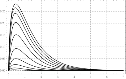
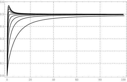
Figure 11: Left: Plots of the truncation error $R_{p}(x/p)$, defined in (124) and (132), as a function of $x$, for various values of $p$. From the highest to the lowest plot: $p\to 0$ (i.e., $xE_{1}(x)$), and $p=0.1,0.2,\ldots,0.9$. We recall that $R_{1}(x)=0$. Right: A similar plot of the KKT gaps attained by the inverse binomial distribution (80).

The error quantity $R_{p}(x)$, depicted in Figure 11, can be shown to be always non-negative:

Claim 33.

For all $x\geq 0$ and $p\in(0,1/2]$, the quantity $R_{p}(x)$ defined in (124) is non-negative.

Proof.

We can rearrange (132) as

$$R_{p}(x) =\int_{p}^{\frac{p}{1-p}}\frac{(1-t)^{x}-(1-p)^{x}}{t\log(1-t)}\,dt-\int_{\frac{p}{1-p}}^{1}\frac{-(1-t)^{x}+(1-p)^{x}+(1-(1-p)t)^{x}-(1-p)^{x}}{t\log(1-t)}\,dt$$

$$=\int_{p}^{\frac{p}{1-p}}\frac{(1-t)^{x}-(1-p)^{x}}{t\log(1-t)}\,dt+\int_{\frac{p}{1-p}}^{1}\frac{(1-t)^{x}-(1-(1-p)t)^{x}}{t\log(1-t)}\,dt,$$

and observe that the integrands inside both integrals in the second equation are non-negative over the integration interval. ∎

In fact, as $p$ gets small, $R_{p}(x)$ converges to $pxE_{1}(px)$, which, as shown in (61), is the gap to equality achieved by the digamma distribution (52) for the mean-limited Poisson channel. This can be seen from the result of Proposition 32 (showing that the truncated distribution for the binomial channel converges to the digamma distribution (52) in the limit $p\to 0$), combined with the fact that the binomial channel converges to a Poisson channel as $p\to 0$.

Using Claim 33 and (131), we now have that, for all integers $x\geq 0$,

$$\mathds{E}[g(Y_{x})]\geq\log x!-\mathcal{E}_{1-p}(x),$$

which, similar to the case $p\geq 1/2$, implies that the probability mass function of $Y$ in (105) satisfies

$$D_{\mathsf{KL}}({Y_{x}}\|{Y})\stackrel{{\scriptstyle\eqref{eqn:bin:KL:general}}}{{=}}-xp\log q-\log y_{0}-R_{p}(x)\leq-xp\log q-\log y_{0},$$

thereby satisfying the KKT conditions (24) for all $x\geq 0$ and with the choices $\nu_{1}=-\log q$ and $\nu_{0}=-\log y_{0}$.

Finally, we derive the asymptotic growth of $g(y)$ using Claim 28 as follows:

$$g(y) =\frac{y}{p}(\log(y/p)+\mathrm{Li}(1-p)-1)-\frac{y(1-p)}{p}\left(\log\left(\frac{(1-p)y}{p}\right)+\mathrm{Li}\left(\frac{1-2p}{1-p}\right)-1\right)$$

$$+\frac{y}{p}\left((1-p)\mathrm{Li}\left(\frac{1-2p}{1-p}\right)-\mathrm{Li}(1-p)\right)+\frac{1}{2}\log(y/p)-\frac{1}{2}\log\left(\frac{(1-p)y}{p}\right)\pm O(1)$$

$$=yh(p)/p+y\log(y/e)+O_{p}(1),$$

which, as was the case for $p\geq 1/2$, confirms that the probability mass function of $Y$ in (105) can be normalized to a legitimate distribution precisely when $q\in(0,1)$, and that the expectation can be adjusted to any desired positive value by choosing $q$ appropriately. The resulting probability mass function of $Y$ is plotted, for various choices of $p$ and $q$, in Figure 12. Furthermore, the mean of the resulting distribution is depicted, for various choices of $p$, in Figure 13.

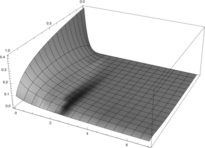
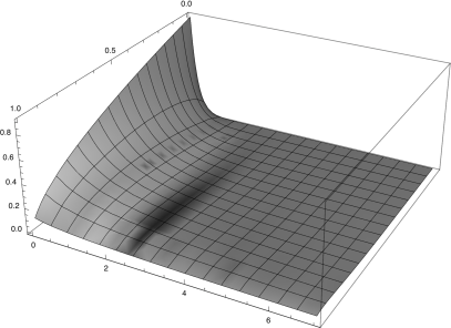
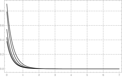
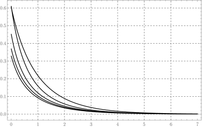
Figure 12: Plots of the probability mass function corresponding to the choice of $Y$ in Theorem 34. For the top plots, the length represents $y$, the width represents $q$, and the height is the probability (left: $p=0.2$, right: $p=0.8$). For the bottom plots, the probability is plotted as a function of $y$, for $p=0.1,0.3,0.5,0.7,0.9$ (from the lowest to the highest curve), where we have chosen $q=0.1$ (left), and $q=0.5$ (right).

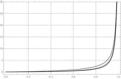
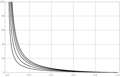
Figure 13: Plots of the mean of the probability distribution corresponding to the choice of $Y$ in Theorem 34. Left: the mean as a function of $q$ for $p=0.1,0.5,0.9$ (from the lowest to the highest curve). Right: the inverse of the mean as a function of $q$ for $p=0.1,0.3,0.5,0.7,0.9$ (from the highest to the lowest curve).

Wrapping up

Equipped with an improved choice for the distribution of the channel output $Y$, we may now proceed as in Section 6.2.1 with the alternative choice applied in Theorem 26, which is restated with the modified distribution below.

Theorem 34.

Let $p\in(0,1)$ and $q\in(0,1)$ be given parameters and $Y$ be a random variable distributed according to (105); that is,

$$\Pr[Y=y]=y_{0}\frac{q^{y}\exp(g(y)-yh(p)/p)}{y!},$$

for an appropriate normalizing constant $y_{0}$ and mean $\mu=\mathds{E}[Y]$, where

$$g(y):=\begin{cases}0&y=0\\ g_{p}(y)&y>0,\end{cases}$$

and $g_{p}(y)$ is defined for $p<1/2$ by (125) and for $p\geq 1/2$ by (121); that is,

$$g_{p}(y):=\begin{cases}\Lambda_{p}(y)-\mathcal{E}_{1/p-1}(y)-y\mathrm{Li}(1-p)/p+\eta(1-p)&p\geq 1/2,\\ \Lambda_{p}(y)-\Lambda_{p/(1-p)}(y)+\frac{y}{p}\left((1-p)\mathrm{Li}\left(\frac{1-2p}{1-p}\right)-\mathrm{Li}(1-p)\right)+\int_{p}^{\frac{p}{1-p}}\frac{dt}{t\log(1-t)}&p<1/2.\end{cases}$$

Then, capacity of the mean-limited binomial channel $\mathsf{Ch}_{\mu}({\mathsf{Ber}}_{p})$ satisfies

$${\mathsf{Cap}}(\mathsf{Ch}_{\mu}({\mathsf{Ber}}_{p}))\leq-\mu\log q-\log y_{0}.$$ (133)

6.3 Derivation of the capacity upper bound for the deletion channel

In order to complete the derivation of the capacity upper bound for the deletion channel, we combine the results of Section 6.2.1, and their improvements in Section 6.2.2, with the general framework developed in Section 4; in particular, Corollary 5.

Denoting by $\mathsf{Ch}$ the deletion channel with deletion probability $d$, and letting $p:=1-d$, the result of Corollary 5 combined with either Theorem 26 or Theorem 34 gives us the capacity upper bound

$${\mathsf{Cap}}(\mathsf{Ch}) \leq\sup_{\mu\geq 0}\frac{{\mathsf{Cap}}(\mathsf{Ch}_{\mu}({\mathsf{Ber}}_{p}))}{1/p+\mu/p}$$

$$\stackrel{{\scriptstyle\eqref{eqn:BinMeanLimCapUpperA}}}{{\leq}}p\,\sup_{q\in(0,1)}\frac{-\mu\log q-\log y_{0}}{1+\mu}=:C_{\mathsf{Ber}}(p),$$ (134)

where $\mu$ and $y_{0}$ respectively denote the mean and normalizing constant of the distribution of $Y$ (defined by either Theorem 26 or Theorem 34) and each depend on both $p$ and $q$. Let $C_{\mathsf{Ber}}(p)$ denote the expression on the right hand side of (134) and $C_{\mathsf{Ber}}(p,q)$ denote the expression inside the supremum in (134). We have proved the following:

Theorem 35.

Let $\mathsf{Ch}$ be a deletion channel with deletion probability $d$, and let $p:=1-d$. Given a parameter $q\in(0,1)$, consider a random variable $Y$ distributed according to either Theorem 26 (inverse binomial) or Theorem 34 (the truncated distribution), with an appropriate normalizing constant $y_{0}(q)$ and mean $\mu(q)=\mathds{E}[Y]$. Then,

$${\mathsf{Cap}}(\mathsf{Ch})\leq C_{\mathsf{Ber}}(1-d)=(1-d)\,\sup_{q\in(0,1)}\frac{-\mu(q)\log q-\log y_{0}(q)}{1+\mu(q)}.$$ (135)

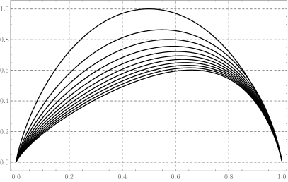
Figure 14: Numerical plots of the capacity upper bound slope $C_{\mathsf{Ber}}(p,q)$ (the expression under the supremum in (134)), measured in bits, for various choices of $p$ and as a function of $q$, where the distribution of $Y$ is given by the inverse binomial distribution in Theorem 26 (left), or the improved (truncated) distribution in Theorem 34 (right). The chosen values for $p$ are (from the lowest to the highest curve): $p=10^{-4},0.1,0.2,\ldots,0.9$, and $p=1$ (in which case the curve is equal to $h(q)$).

 

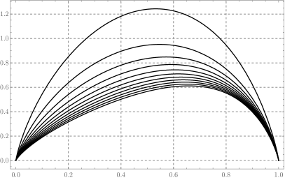
Figure 15: Analytic upper bounds on the capacity slope $C_{\mathsf{Ber}}(p,q)$ (the expression under the supremum in (134)), measured in bits, for various choices of $p$ and as a function of $q$, where the distribution of $Y$ is given by the inverse binomial distribution in Theorem 26. The diagram on the left plots the upper bound on $C_{\mathsf{Ber}}(p,q)$ in terms of elementary functions, using Corollary 22. The diagram on the right uses the upper bounds in terms of standard special functions given by Theorem 24. The choices of $p$ are, from the lowest curve to the highest: $p=10^{-4},0.1,0.2,\ldots,0.9$, and $p=0.999$ (the latter being excluded in the first diagram as the resulting capacity upper bounds are already trivial at $p=0.9$).

 

Note that, when $p=1$, both Theorem 26 and Theorem 34 assign a geometric distribution to $Y$. As we show in Section 6.3.4, in both cases we have $C_{\mathsf{Ber}}(1,q)=h(q)$.

6.3.1 The particular case $d=1/2$

Recall that, for the special case $p=d=1/2$, the inverse binomial distribution defined in (80) becomes, precisely, a negative binomial distribution. Thus, in this case, the right hand side of (135) can be analytically optimized in closed form. Using (83), the expression under supremum is equal to

$$C_{\mathsf{Ber}}(1/2,q)=\frac{-\frac{q}{2(1-q)}\log q-\log\sqrt{1-q}}{1+\frac{q}{2(1-q)}}=\frac{h(q)}{2-q},$$ (136)

whose maximum is attained at the golden ratio conjugate $q=(\sqrt{5}-1)/2$ (shown by equating the derivative of the expression to zero, which results in a quadratic equation). It can be verified by straightforward manipulations that, in this case, the resulting capacity upper bound given by (135) is equal to

$$C_{\mathsf{Ber}}(1/2)=\frac{1}{4}\log\frac{3+\sqrt{5}}{2}=\frac{1}{2}\log\varphi\approx 0.347120\ \text{\rm(in bits per channel use)},$$ (137)

where $\varphi=(1+\sqrt{5})/2$ is the golden ratio.

An extension of the above result for $p=1/2$ to smaller values of $p$ is presented in Appendix B.5. However, the convexification result of [ref:RD15] may be used along with our capacity upper bound for $d=p=1/2$ to derive simple and closed-form capacity upper bounds for general deletion probabilities. Namely, we prove the following:

Corollary 36.

Let $\mathsf{Ch}$ be the deletion channel with deletion probability $d$. Then,

$${\mathsf{Cap}}(\mathsf{Ch})\leq\begin{cases}(1-d)\log\varphi\approx 0.694242(1-d)&d\geq 1/2,\\ 1-d\log(4/\varphi)\approx 1-1.305758d&d<1/2,\\ \end{cases}$$

where $\varphi=(1+\sqrt{5})/2$ is the golden ratio, the entropy is in bits per channel use, and the bound for $d<1/2$ holds under the plausible conjecture [ref:Dal11] that the capacity function is convex over $d\in[0,1/2]$.

Proof.

Suppose that capacity upper bounds of $c_{1}$ and $c_{2}$, respectively for deletion probabilities $d_{1}$ and $d_{2}$ are known. Let $\ell\in(0,1)$ and $c$ be the capacity of the channel at deletion probability $d:=\ell d_{1}+(1-\ell)d_{2}$. Under the assumption that the capacity function for the deletion channel is a convex function of $d$, it would trivially follow that $c\leq\ell c_{1}+(1-\ell)c_{2}$, hence proving the claim by letting $d_{1}=1/2$, $c_{1}=(\log\varphi)/2$, and either $d_{2}=0$ with $c_{2}=\log 2$ or $d_{2}=1$ with $c_{2}=0$. Without assuming the convexity conjecture, it has been shown in [ref:RD15, Theorem 1] that, unconditionally, one has (with entropy measured in bits)

$$c\leq\ell c_{1}+(1-\ell)c_{2}+(1-d)\log(1-d)-\ell(1-d_{1})\log(\ell(1-d_{1}))-(1-\ell)(1-d_{2})\log((1-\ell)(1-d_{2})).$$

By letting $d_{2}=1$ and $c_{2}=0$, and $d=\ell d_{1}+(1-\ell)$ (thus, $1-d=\ell(1-d_{1})$) one gets $c\leq\ell c_{1}+\ell(1-d_{1})\log(\ell(1-d_{1}))-\ell(1-d_{1})\log(\ell(1-d_{1}))=\ell c_{1}$, proving the unconditional claim for $d\geq 1/2$. We remark that one could use the result of [ref:RD15] with $d<1/2$ and get nontrivial upper bounds, unconditionally, for a range of $d$ below $1/2$ as well (e.g., $d\geq 0.48$). ∎

6.3.2 The general case.

For general $p$, the function $C_{\mathsf{Ber}}(p,q)$, under both Theorems 26 and 34, is numerically plotted in Figure 14. Furthermore, if Theorem 26 is used to determine the distribution of $Y$ (i.e., the inverse binomial distribution), high-quality upper bound estimates on the value of $C_{\mathsf{Ber}}(p,q)$ in terms of elementary or standard special functions (when $p$ is not too close to $1$) are available via Corollary 22 and Theorem 24. These upper bounds are plotted in Figure 15.

Maximizing the value of $C_{\mathsf{Ber}}(p,q)$ with respect to $q$ for a given $p=1-d$ results in capacity upper bounds for the deletion channel with deletion probability $d$. The quality of the upper bound depends on the result used to determine $C_{\mathsf{Ber}}(p,q)$, including, and in decreasing order of quality:

1. Theorem 34 for the distribution of $Y$ (i.e., the truncated distribution),

2. Theorem 26 for the distribution of $Y$ (i.e., the inverse binomial distribution),

3. The analytic upper bound estimates of Theorem 24 on the inverse binomial distribution,

4. The elementary upper bound estimates of Corollary 22 on the parameters of the inverse binomial distribution.

Plots of the resulting capacity upper bounds for general $d$ are given in Figure 16, and are compared with the best available capacity upper bounds as reported in [ref:RD15] (which are, in turn, based on the results of [ref:FD10] combined with a convexification technique). The corresponding numerical values for the plotted curves are also listed, for various choices of the deletion probability $d$, in Table B.5.

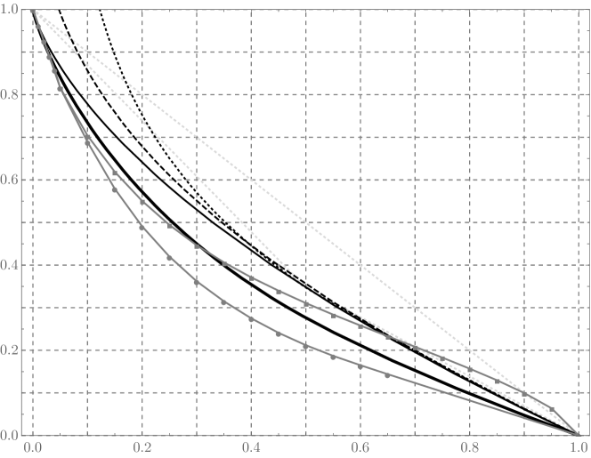
Figure 16: Upper bounds (in bits per channel use) on the capacity of the deletion channel, plotted as a function of the deletion probability $d$. The bounds are obtained using i) Theorem 34 (solid, thick), ii) Theorem 26 (solid, black), iii) analytic upper bound estimates of Theorem 24 (dashed, black), iv) elementary upper bound estimate of Corollary 22 (dotted, black). The best known capacity upper bounds reported in [ref:RD15] are shown in gray with the circle markers representing the explicitly reported data points. The gray plot with square markers are the upper bounds reported in [ref:MDP07]. The trivial erasure capacity upper bound $1-d$ as well as the fully analytic upper bounds of Corollary 36 are displayed in dotted light gray. The numeric values corresponding to the plots are listed in Table B.5.

 

6.3.3 The limiting case $d\to 1$

When the deletion probability $d$ tends to $1$, or equivalently $p=1-d\to 0$, the capacity upper bounds take the form $C_{\mathsf{Ber}}(p)\leq C_{0}(1-d)$, for an absolute constant $C_{0}$. The value of $C_{0}$ depends on which one of the above four results is used, and by numerically maximizing the univariate concave function $C_{\mathsf{Ber}}(p,q)$ over $q\in(0,1)$, can be approximated, respectively, as follows (measured in bits):

1. Under Theorem 34, $C_{0}\approx 0.4644$ with maximizer $q\approx 0.7247$,

2. Under Theorem 26, $C_{0}\approx 0.6015$ with maximizer $q\approx 0.6590$,

3. Using the analytic upper bound estimate of Theorem 24, $C_{0}\approx 0.6115$ with maximizer $q\approx 0.6573$,

4. Using the elementary upper bound estimate of Corollary 22, $C_{0}\approx 0.6196$ with maximizer $q\approx 0.6644$.

We also recall that, as we saw in the result of Section 6.3.1 for the particular case $d=1/2$, the fully explicit upper bound of $(\log\varphi)/2$ for this case can be linearly extended to all $d\geq 1/2$, including the limiting case $d\to 1$, using the convexification technique of [ref:RD15]. Indeed, Corollary 36 implies the choice of $C_{0}=\log\varphi\approx 0.694242(1-d)$ (in bits), where $\varphi$ is the golden ratio, for this case.

Remark 37.

We remark that the above upper bound estimate of $0.4644(1-d)$ for $d\to 1$ coincides with what we achieve for the Poisson-repeat channel with the same deletion probability in Corollary 19. This is due to the fact that the truncated distribution (52) (the digamma distribution) for the Poisson-repeat channel is the limiting distribution of what we obtain in Section 6.2.2 using the truncation method (as shown by Proposition 32), and that the mean-limited binomial channel converges a mean-limited Poisson channel in the limit $d\to 1$.

6.3.4 The limiting case $d\to 0$

The limiting behavior of the capacity of the deletion channel for $d\to 0$ is very well understood [ref:KMS10, ref:KM13]. In particular, in this case, it is known that the capacity behaves as $1-h(d)+O(d)=1+d\log d+O(d)$ (in bits per channel use). The goal of this section is to prove that the capacity upper bounds obtained by Theorem 35 exhibit the correct asymptotic behavior of $1-\Theta(h(d))$ for small $d$ (albeit with a slightly sup-optimal constant behind $h(d)$). We demonstrate the result for Theorem 35 applied with the weaker choice of the inverse binomial distribution. The same approach could be used to obtain an analogous results for the truncated distribution of Theorem 34.

Theorem 38.

Consider the deletion channel $\mathsf{Ch}$ with deletion probability $d\to 0$. Then, the capacity upper bound of Theorem 35 with respect to the inverse binomial distribution (80) takes the form

$${\mathsf{Cap}}(\mathsf{Ch})\leq 1-(1-O(d))h(d)/2=1-h(d)/2+o(d)\text{ (bits per channel use)}.$$

Proof.

Let $Y$ be an inverse binomial random variable with parameter $q$, normalizing constant $y_{0}$ and mean $\mu:=\mathds{E}[Y]$. We first recall (134), that

$${\mathsf{Cap}}(\mathsf{Ch})\leq(1-d)\,\sup_{q\in(0,1)}\frac{-\mu\log q-\log y_{0}}{1+\mu}.$$

We first rule out the possibility of the optimum $q$ being close to $1$ (which is evident from Figure 15). This is immediate from the estimates on the parameters of an inverse binomial distribution given by Corollary 22. Namely, Corollary 22 proves that, when $q\to 1$, we have $-\log y_{0}=O(-\log(1-q))$, and $\mu=\Omega(1/(1-q))$. Thus, in this regime we have

$$\frac{-\mu\log q-\log y_{0}}{1+\mu}\leq-\log q-\frac{\log y_{0}}{\mu}=-\log q+O(-(1-q)\log(1-q))=O(h(q))\to 0.$$

Without loss of generality we may therefore assume that there is an absolute constant $q_{0}<1$ such that $q\leq q_{0}$ (since we now know that the supremum in (134) over the values of $q$ close to $1$ approaches zero). Logarithm of the binomial coefficient $\binom{y/p}{y}$ admits the series expansion (in $d$)

$$\log\binom{\frac{y}{1-d}}{y}=(\gamma+\psi(y+1))yd+\frac{y}{12}\left(12\gamma+12\psi(y+1)-\pi^{2}y+6\psi^{\prime}(y+1)y\right)d^{2}+O(d^{3}y^{2}+d^{4}y^{4})+\cdots,$$

where $\gamma$ is the Euler-Mascheroni constant, and $\psi$ is the digamma function. Consider a parameter $y_{1}=O(\log(1/d))$ to be determined later. For any $y\leq y_{1}$, we may thus write

$$1\leq\binom{\frac{y}{1-d}}{y}\leq 1+O(dy\log y)=1+O(dy^{2}).$$

From the definition of the inverse binomial distribution (80), and the above estimate, we may write

$$y_{0}q^{y}\exp(-yh(d)/(1-d))\leq\Pr[Y=y]\leq y_{0}q^{y}\exp(-yh(d)/(1-d))(1+O(dy^{2}))$$ (138)

for all $y\leq y_{1}$. We also recall that, letting $\delta:=\exp(-h(d)/(1-d))$, for all $y\geq 0$,

$$\binom{\frac{y}{1-d}}{y}\leq\exp(yh(1-d)/(1-d))=1/\delta^{y},$$ (139)

and thus, for all $y\geq 0$,

$$\Pr[Y=y]/y_{0}=\binom{\frac{y}{1-d}}{y}(\delta q)^{y}\stackrel{{\scriptstyle\eqref{eqn:binom:upper}}}{{\leq}}q^{y}.$$ (140)

Since $1-q=\Omega(1)$, we may choose $y_{1}$ large enough so as to ensure that

$$\sum_{y=y_{1}}^{\infty}y\Pr[Y=y]/y_{0}\leq dq<d.$$ (141)

In the sequel, we use asymptotic notation with respect to the vanishing parameter $d$; i.e., $d=o(1)$. We may write,

$$1/y_{0} =\sum_{y=0}^{\infty}\Pr[Y=y]/y_{0}$$

$$=\sum_{y=0}^{\infty}\binom{\frac{y}{1-d}}{y}(\delta q)^{y}$$

$$\stackrel{{\scriptstyle\eqref{eqn:ibin:tail}}}{{\leq}}d+\sum_{y=0}^{y_{1}}\binom{\frac{y}{1-d}}{y}(\delta q)^{y}$$

$$\leq d+\sum_{y=0}^{\infty}(\delta q)^{y}(1+O(dy^{2}))$$

$$=d+\frac{1}{1-\delta q}+O\left(\frac{d\delta q(1+\delta q)}{(1-\delta q)^{3}}\right)$$

$$\leq d+\frac{1}{1-\delta q}\left(1+O\left(\frac{d\delta q}{(1-\delta q)^{2}}\right)\right)$$

$$\leq\frac{1+O(d)}{1-\delta q},$$

where in the last inequality we have used the assumptions $q\leq q_{0}$, $1-q_{0}=\Omega(1)$, $d=o(1)$, and $\delta=1-\Theta(d\log d)=1-o(1)$. Upper bounding $y_{0}$ is slightly simpler:

$$1/y_{0}=\sum_{y=0}^{\infty}\Pr[Y=y]/y_{0} \geq\sum_{y=0}^{\infty}(q\delta)^{y}=\frac{1}{1-\delta q}.$$

Using a similar approach, we may upper bound $\mu$ as follows:

$$\mu/y_{0} =\sum_{y=1}^{\infty}y\Pr[Y=y]/y_{0}$$

$$\stackrel{{\scriptstyle\eqref{eqn:ibin:tail}}}{{\leq}}dq+\sum_{y=1}^{y_{1}}y\Pr[Y=y]/y_{0}$$

$$\leq dq+\sum_{y=1}^{\infty}y(\delta q)^{y}(1+O(dy^{2}))$$

$$=dq+\frac{\delta q}{(1-\delta q)^{2}}+O\left(\frac{d(\delta^{2}q^{2}+4\delta q+1)}{(1-\delta q)^{4}}\right)$$

$$\leq dq+\frac{\delta q}{(1-\delta q)^{2}}\left(1+O\left(\frac{d}{(1-\delta q)^{2}}\right)\right)$$

$$\leq\frac{\delta q}{(1-\delta q)^{2}}(1+O(d)),$$

so that, using the upper bound on $y_{0}$,

$$\mu\leq\frac{\delta q(1+O(d))}{1-\delta q}.$$

Finally, we lower bound $\mu$ as

$$\mu/y_{0}=\sum_{y=1}^{\infty}y\Pr[Y=y]/y_{0} \geq\sum_{y=1}^{\infty}y(q\delta)^{y}=\frac{\delta q}{(1-\delta q)^{2}},$$

and using the lower bound on $y_{0}$, we write

$$\mu\geq\frac{\delta q(1-O(d))}{1-\delta q}.$$

In conclusion, we have so far shown the estimates

$$y_{0}=(1-\delta q)(1-O(d)),\quad\mu=\frac{\delta q(1\pm O(d))}{1-\delta q}$$ (142)

We are now ready to apply the above estimates in (134), and write

$${\mathsf{Cap}}(\mathsf{Ch}) \leq(1-d)\,\sup_{q\in(0,1)}\frac{-\mu\log q-\log y_{0}}{1+\mu}$$

$$\leq\sup_{q\in(0,q_{0})}\frac{-\mu\log q-\log y_{0}}{1+\mu}$$

$$\stackrel{{\scriptstyle\eqref{eqn:ibin:geom:c}}}{{\leq}}\sup_{q\in(0,q_{0})}(1-\delta q)\frac{-\frac{\delta q}{1-\delta q}\log q-\log(1-\delta q)\pm O(d)}{1\pm O(d)}\,(1+O(d))$$

$$\leq\sup_{q\in(0,q_{0})}(h(\delta q)+\delta q\log\delta\pm O(d))\,(1+O(d))$$

$$\leq\sup_{q\in(0,q_{0})}(h(\delta q)-\delta qh(d)/(1-d)\pm O(d))\,(1+O(d))$$

$$\leq\sup_{q\in(0,q_{0})}(h(\delta q)-\delta qh(d)\pm O(d))\,(1+O(d)).$$

In the above result, the expression under the supremum approaches zero for $q\to 0$, and approaches one for $\delta q=1/2$. Therefore, we expect the supremum to occur around $q\approx 1/2$ and be close to one. In particular, we know that the supremum is away from zero (by a constant), and may thus write the above as

$${\mathsf{Cap}}(\mathsf{Ch})\leq(1+O(d))\sup_{q\in(0,q_{0})}(h(\delta q)-\delta qh(d)).$$ (143)

Consider the function $c(\rho):=h(\rho)+\epsilon\rho$. By simply equating the derivative of the function to zero, it follows that the maximum of this function is attained at $\rho^{\star}=e^{\epsilon}/(1+e^{\epsilon})$ and the that maximum value is

$$c^{\star}=\frac{e^{\epsilon}(\epsilon+\log(1+e^{-\epsilon}))+\log(1+e^{\epsilon})}{1+e^{\epsilon}}=\log 2+\epsilon/2+\epsilon^{2}/8-O(\epsilon^{4}).$$

By letting $\rho:=\delta q$ and $\epsilon:=-h(d)$, we conclude that

$$\eqref{eqn:ibin:geom:d}\leq(\log 2-h(d)/2)(1+O(d))=\log 2-(1-O(d))h(d)/2,$$

as desired. ∎

7 Discussion and open problems

We introduced a number of new techniques that leave plenty of room for improvement in execution and lead to intriguing problems for future investigation. The first is to understand the loss in the capacity upper bound (1). Recall that the Markov chain representation $X-Z-Y$ of a $\mathcal{D}$-repeat channel in Section 2.1 (Figure 1) is exact. However, as shown in (26), the potential loss would correspond to the term $I(Y;Z|X)$. Developing techniques for lower bounding this conditional mutual information for the optimal input distribution $X$ would readily yield an improvement in the capacity upper bound (assuming that one can show a general $\Omega(n)$ lower bound on this conditional mutual information).

Another intriguing problem is to further improve the quality of the dual feasible distributions that we introduced for the Poisson-repeat and deletion channels (i.e., the digamma distribution (5) and the truncated variation of (8)). Can the truncation technique of Sections 5.2 and 6.2.2 be further refined to result in even better capacity upper bounds for either channel? As we observe in Remarks 12 and 30, the optimal input distributions for mean-limited Poisson and binomial channels cannot have full support on all non-negative integers, although they must have infinite supports. Our intuition based on the variances suggests that the optimal input distribution must actually be quite sparse; e.g., supported on points $\Theta(i^{2}/\lambda)$ for the Poisson case and $\Theta(i^{2}(1-p)/p)$ for the binomial case ($i=0,1,\ldots$). A further intuition is that the KKT gap in (2) attained by the optimal output distribution should take the general form of the gaps attained by our dual-feasible distributions (Figures 2 and 11), but additionally, oscillate back and forth to zero (while remaining positive) and reach zero exactly at the sparse set of points supported by the optimal input distribution.

In the $X-Z-Y$ Markov chain representation of the deletion channel (Figure 1), observe that each $Z_{i}$ is the sum of a geometric number of the entries in the run-length representation ${X_{1}},{X_{2}},\ldots,{X_{t}}$ of $X$, and that $Y_{i}$ is obtained by passing $Z_{i}-1$ through a binomial channel. Let $Z^{\star}$ be the optimal input distribution for a single use of the binomial channel, and $\chi$ be the characteristic function of the distribution of $1+Z^{\star}$. We say the distribution is geometrically infinitely divisible if $e^{1-1/\chi(t)}$ is an infinitely divisible characteristic function [ref:KMM85]. In this case, for all $r\in(0,1]$, one can identify a random variable $Z^{\prime}$ such that $1+Z^{\star}$ is the sum of a geometric number (with mean $1/r$) of independent copies of $Z^{\prime}$. Then, one may hope to set up the run-length distribution of the input sequence $X$ to be i.i.d. from a distribution $X^{\prime}$ such that, for an appropriate $r$, sum of a geometric (with mean $1/r$) copies of $X^{\prime}$ gives the distribution of $1+Z^{\star}$. If $r$ is chosen appropriately (i.e., such that it coincides with the deletion probability of an entire run in $X$), the distribution of $Z_{1}-1,Z_{2}-1,\ldots$ would form a sequence of i.i.d. copies of $Z^{\star}$; i.e., the optimal input distribution for the $Z-Y$ link. In this case, one may hope to show that the resulting input distribution $X$ would be capacity achieving for the deletion channel. We note, however, that currently there is no general consensus on whether the capacity achieving input distribution for the deletion channel must consist of i.i.d. run-lengths. This is known to be the case for $d\to 0$ [ref:KM13]. The optimality of i.i.d. run-lengths has not been ruled out for any $d$, and indeed the above intuition on geometric infinite divisibility may suggest this as a possibility.

We obtain sharp estimates on the functions inside the supremums in (4) and (7) in terms of elementary or standard special functions. Can the supremums themselves (i.e., the capacity upper bounds) be upper bounded in terms of such explicit functions? An effort towards this goal is demonstrated in Appendix B.5. Furthermore, our work motivates the study of several novel discrete probability distributions that are worth further consideration.

Appendix A Proof of Theorem 13

Our starting point is the Stirling approximation of the gamma function

$$n!=\Gamma(n+1)\sim\sqrt{2\pi n}\left(\frac{n}{e}\right)^{n},$$

which asymptotically matches $n!$ and, for all $n>0$, provides a lower bound on $n!$. A generalized form of the approximation is

$$n!\sim\sqrt{2\pi(n+\sigma)}\left(\frac{n}{e}\right)^{n},$$ (144)

for some real parameter $\sigma\geq 0$, so the Stirling approximation is the special case $\sigma=0$. By “fine tuning” the constant $\sigma$, it is possible to obtain sharp lower bounds, and upper bounds, on $n!$ for all $n\geq 1$. Lets us call a value of $\sigma$ a lower (resp., upper) bounding constant for (144) if the resulting estimate provides a lower (resp., upper) bound on $n!$ for all $n\geq 1$. It was shown by Gosper [ref:Gos78] that $\sigma=1/6\approx 0.166$ provides a remarkably accurate lower bound estimate on $n!$. The accuracy of this estimate has been studied in [ref:Nem11], where it is shown that

$$\Gamma(n+1)=\left(\frac{n}{e}\right)^{n}\sqrt{2\pi(x+1/6)}\left(1+\frac{1}{144(n+1/4)^{2}}-\frac{1}{12960(n+1/4)^{3}}-\cdots\right),$$

leading to a multiplicative error of about $0.4\%$ even for $n=1$ (as opposed to about $8\%$ achieved by the Stirling approximation). Let us consider fixed choices of lower and upper bounding constants, respectively, $\underline{\sigma}$ and $\overline{\sigma}$, for (144). By inspection, we find that the following are valid choices

$$\underline{\sigma}:=1/6=15/90,\quad\overline{\sigma}:=0.177\approx 16/90.$$ (145)

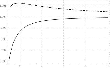
Figure 17: Plot of $\left(\sqrt{2\pi(n+\sigma)}\left(\frac{n}{e}\right)^{n}\right)/\Gamma(n+1)$, as a function of $n\geq 1$, with $\sigma=\underline{\sigma}$ (solid) and and $\sigma=\overline{\sigma}$ (dashed) as determined by (145).

Now, let us define functions

$$S_{0}(q) :=\sum_{y=1}^{\infty}\frac{y^{y}}{y!}\,(q/e)^{y},$$

$$S_{1}(q) :=\sum_{y=1}^{\infty}\frac{y^{y+1}}{y!}\,(q/e)^{y}.$$

Using (144), we can compute upper and lower bounds on the values of these functions as follows. Define

$$S_{0}(q,\sigma) :=\sum_{y=1}^{\infty}\frac{y^{y}}{\sqrt{2\pi(y+\sigma)}\left(\frac{y}{e}\right)^{y}}\,(q/e)^{y}$$ (146)

$$=\frac{1}{\sqrt{2\pi}}\sum_{y=1}^{\infty}\frac{q^{y}}{\sqrt{y+\sigma}}$$

$$=\frac{q}{\sqrt{2\pi}}\Phi(q,1/2,1+\sigma),$$ (147)

where $\Phi(\cdot)$ denotes the Lerch transcendent (62). For the special case $\sigma=0$, this slightly simplifies to

$$S_{0}(q,0)=\frac{1}{\sqrt{2\pi}}\mathrm{Li}_{1/2}(q),$$

where $\mathrm{Li}_{s}(\cdot)$ denotes the polylogarithm function

$$\mathrm{Li}_{s}(z):=\sum_{k=1}^{\infty}z^{k}k^{-s}.$$ (148)

Similarly, we define

$$S_{1}(q,\sigma) :=\sum_{y=1}^{\infty}\frac{y^{y+1}}{\sqrt{2\pi(y+\sigma)}\left(\frac{y}{e}\right)^{y}}\,(q/e)^{y}$$ (149)

$$=\frac{1}{\sqrt{2\pi}}\sum_{y=1}^{\infty}\frac{(y+\sigma-\sigma)q^{y}}{\sqrt{y+\sigma}}$$

$$=\frac{q}{\sqrt{2\pi}}\Phi(q,-1/2,1+\sigma)-\sigma S_{0}(q,\sigma),$$ (150)

which, for $\sigma=0$, simplifies to

$$S_{1}(q,0)=\frac{1}{\sqrt{2\pi}}\mathrm{Li}_{-1/2}(q).$$

Clearly, we have

$$S_{0}(q)\geq S_{0}(q,\overline{\sigma}),\quad S_{1}(q)\geq S_{1}(q,\overline{\sigma}),\quad S_{0}(q)\leq S_{0}(q,\underline{\sigma}),\quad S_{1}(q)\leq S_{1}(q,\underline{\sigma}).$$ (151)

Given a parameter $q\in(0,1)$, using $\eqref{eqn:PoiYfirst}$ we may write

$$y_{0}=1/(1+S_{0}(q)),\quad\mu:=\mathds{E}[Y]=y_{0}S_{1}(q)=S_{1}(q)/(1+S_{0}(q)).$$

Using (147) and (150), we may now derive the estimates (63) in the statement. This completes the proof.

Appendix B Analytic claims

In this section, we verify a number of stand-alone analytic claims that have been used in the proofs.

B.1 Claim 15

Consider the derivative of the function $g$ defined in (68):

$$g^{\prime}(y) =\frac{1}{\sqrt{\pi}}\left(\Gamma^{\prime}(y+1/2)\exp(y-y\psi(y))+\Gamma(y+1/2)\exp(y-y\psi(y))(1-(\psi(y)+y\psi^{\prime}(y)))\right)$$

$$=\frac{-1}{\sqrt{\pi}}\Gamma(y+1/2)\exp(y-y\psi(y))\,(-\psi(y+1/2)-1+\psi(y)+y\psi^{\prime}(y)),$$

where $\psi(\cdot)$ is the digamma function. It can be seen that the function

$$\varphi(y):=-\psi(y+1/2)+\psi(y)+y\psi^{\prime}(y)-1,$$ (152)

depicted in Figure 18, is positive for all $y>0$ (in fact, this function is completely monotone, which can be proved by expressing $\varphi(y)$ using Euler’s integral representation for the digamma function). It follows that $g^{\prime}(y)<0$ for all $y>0$, and thus the ratio $g$ is strictly decreasing.

Figure 18: Plot of the function $\varphi$ in (152).

B.2 Claim 20

For the special case $p=1/2$, the ratio is equal to $1$ for all $y>0$ due to the duplication formula for the gamma function:

$$\Gamma(y)\Gamma\left(y+{\tfrac{1}{2}}\right)={\sqrt{4\pi}}\;\Gamma(2y)/4^{y},$$

which implies that,

$$\binom{2y}{y}=\frac{2\Gamma(2y)}{\Gamma(y)\Gamma(y+1)}=\frac{4^{y}\Gamma(y+\frac{1}{2})}{\sqrt{\pi}\Gamma(y+1)}=\frac{4^{y}}{\sqrt{\pi}}\binom{y-\frac{1}{2}}{y}\Gamma(1/2)=4^{y}\binom{y-\frac{1}{2}}{y},$$

and the result follows by noting that $h(1/2)=\log 2$. Since $\rho$ is always positive for $y>0$, it is increasing (decreasing) if and only if $\log\rho$ is increasing (decreasing). We can write the derivative of $\log\rho$ in $y$ by taking the derivative of each constituent term; that is,

$$p\frac{d}{dy}\log\rho(y)=-h(p)-p\psi(y+1/2)-(1-p)\psi(y(1/p-1)+1)+\psi(y/p+1)=:\rho_{1}(y).$$

One can verify that $\lim_{y\to\infty}\rho_{1}(y)=0$. The derivative of $\rho_{1}(y)$, in turn, can be written as

$$p\frac{d}{dy}\rho_{1}(y)=-p^{2}\psi^{\prime}(y+1/2)-(1-p)^{2}\psi^{\prime}(y(1/p-1)+1)+\psi^{\prime}(y/p+1).$$

This function is positive and decreasing in $y$ (in fact, completely monotone) when $p<1/2$, identically zero when $p=1/2$, and negative and increasing (in fact, negated completely monotone) when $p>1/2$ (this can be proved using Theorem 39). It follows that $\rho_{1}(y)$ is increasing (and negative) when $p<1/2$, zero when $p=1/2$, and decreasing (and positive) when $p>1/2$. The claim follows.

B.3 Claim 23

We do not present a rigorous proof that the particular choices of $\overline{\alpha}$ and $\underline{\alpha}$ in the statement are valid, but rather, provide a convincing argument. It would be an interesting question to provide a complete proof. Consider the log-ratio

$$R_{p,\alpha}(y):=\log\binom{y/p}{y}-yh(p)/p+\frac{1}{2}\log(2\pi((1-p)y+\alpha)).$$ (153)

By Stirling’s approximation, it follows that for any $p\in(0,1)$ and any fixed $\alpha$, we have

$$\lim_{y\to\infty}R_{p,\alpha}(y)=0.$$

It can be proved, using Theorem 39, that the function $-R_{p,0}$ is completely monotone for all $p\in(0,1)$. Therefore, even for $y\geq 0$, the constant $\alpha=0$ provably provides an upper bound for $\binom{y/p}{y}$. That is, for all $p\in(0,1)$,

$$\binom{y/p}{p}\leq\frac{\exp(yh(p)/p)}{\sqrt{2\pi(1-p)y}}.$$

We now have the more refined task of finding choices of $\alpha$ that makes the above log-ratio always positive (negative) for all $p\in(0,1)$ and all $y\geq 1$ (rather than $y\geq 0$). It is worthwhile to note that the $j$th derivative of the function $-R_{p,\alpha}(y)$ (for $j\geq 1$) can be computed, letting $q:=p/(1-p)$, as

$$\frac{A_{j-1}(-p)^{j}(1-p)^{j}+(a+y(1-p))^{j}(p^{j}\psi^{(j-1)}(1+y)-\psi^{(j-1)}(1+\frac{y}{p})+(1-p)^{j}\psi^{(j-1)}(1+\frac{y}{q}))}{p^{j}(a+y(1-p))^{j}},$$

where $\psi^{(j)}$ is the polygamma function, $A_{j}$ is the number of even permutations on $n$ items (OEIS A001710), except for the special cases $A_{1}:=A_{0}:=1/2$, and that for the first derivative, an additional constant $h(p)/p$ is to be added to the above expression to obtain the correct derivative. Figure 19 depicts the log-ratio function and its derivative for various choices of $\alpha$ and $p$. At $y=1$, we have

$$R_{p,\alpha}(1)=(1-p)\log(1-p)/p+\log(2\pi(1-p+\alpha))/2.$$

By setting $R_{p,\alpha}(1)=0$, and solving for $\alpha$, we obtain the solution

$$\alpha_{0}:=-1+p+\frac{(1-p)^{2-2/p}}{2\pi}.$$

The value of the solution $\alpha_{0}$ as a function of $p$ is plotted in Figure 19 (the limit at $p\to 0$ is $e^{2}/(2\pi)-1\approx 0.176$, and the minimum occurs a $p\approx 0.405$ at which point we have $\alpha_{0}\approx 0.136$). Note that $\alpha_{0}$ is the transition point for whether the plot for the log-ratio lies above or below the horizontal axis around $y=1$, and we see that this transition always occurs within $\alpha\in(0.13,0.18)$. By choosing the value of $\alpha$ sufficiently outside this critical region (in particular, for the choices of $\underline{\alpha}$ and $\overline{\alpha}$ in the statement), we may ensure that the log-ratio remains above, or below, zero for $y\geq 1$ until the asymptotic convergence towards zero dominates the behavior of the function. The log-ratios for the chosen values of $\underline{\alpha}$ and $\overline{\alpha}$ and various choices of $p$ are plotted as functions of $y$ in Figure 19. We observe that, apart from the cases $p\to 0$ and $p\to 1$, the log-ratio $R_{p,\alpha}(y+1)$ or its negation appear to be not only positive, but also completely monotone for the chosen values of $\alpha$.

Figure 19: Plots related to the log-ratio function $R_{p,\alpha}$ in (153). Top: plots of $R_{0.5,\alpha}(y)$, as functions of $y$, for $\alpha=0.1,0.15,0.20,0.25,0.30$ (left, from the lowest to the highest curve) and their derivatives in $y$ (right, from the highest to the lowest curve). Bottom left: plot of $\alpha_{0}=-1+p+(1-p)^{2-2/p}/(2\pi)$ as a function of $p$. Bottom right: plots of $R_{p,\underline{\alpha}}(y)$ (solid) and $R_{p,\overline{\alpha}}(y)$ (dashed) in $y$ for $p=10^{-3},10^{-2},0.1,0.3,0.5,0.7,0.9,0.99,0.999$.

B.4 Claim 25

In this section, we prove Claim 25 that is restated below:

Claim.

The function

$$f(y):=\log\binom{y}{py}=\log\frac{\Gamma(y+1)}{\Gamma(py+1)\Gamma((1-p)y+1)},$$

defined for $p\in(0,1)$ and $x>0$, is completely monotone. That is, for all integers $j=0,1,\ldots$, $(-1)^{j}f^{(j)}(y)>0$ for all $y>0$.

Proof.

By definition, $f(y)>0$ for all $y>0$. Moreover, $f^{\prime}(y)=\psi(y+1)-p\psi(py+1)-(1-p)\psi((1-p)y+1)$, which is positive for all $y>0$ by the concavity of the digamma function. Thus, it suffices to show that $f^{\prime\prime}(y)$ is completely monotone. This claim is a special case of the following result proved in [ref:KP16]:

Theorem 39.

[ref:KP16] Let

$$F(y):=\frac{\Pi_{i=1}^{m}\Gamma(A_{i}y+a_{i})}{\Pi_{j=1}^{n}\Gamma(B_{j}+b_{j})}.$$

Then, $(\log F(y))^{\prime\prime}$ is completely monotone if and only if the function

$$P(u):=\sum_{i=1}^{m}\frac{\exp(-a_{i}u/A_{i})}{1-\exp(-u/A_{i})}-\sum_{i=1}^{n}\frac{\exp(-b_{j}u/B_{j})}{1-\exp(-u/B_{j})}$$

is non-negative for all $u>0$. ∎

For our application, we have

$$P(u)=\frac{1}{e^{u}-1}-\frac{1}{e^{u/p}-1}-\frac{1}{e^{u/q}-1}.$$

In order to show that $P(u)\geq 0$, it suffices to verify that

$$P_{0}(u):=\frac{p}{e^{u}-1}-\frac{1}{e^{u/p}-1}\geq 0$$

for all $u>0$, or equivalently, that $pe^{u/p}-e^{u}+1-p\geq 0$ for all $u>0$. The left hand side is zero at $u=0$ and has a positive derivative in $u$ (which is $e^{u/p}-e^{u}$) for all $u\geq 0$. The result follows. ∎

B.5 An analytically simple deletion capacity upper bound for $p\leq 1/2$

In this appendix, we show that the result of (136) for $p=1/2$ can be extended to smaller values of $p$ as well, leading to simple and analytic capacity upper bound expressions. In particular, recalling the notation of Section 6.3, we observe the following:

Claim 40.

Let $C_{\mathsf{Ber}}(p,q)$ be defined with respect to the inverse binomial distribution for $Y$. Then, for all $p\leq 1/2$, and all $q\in(0,1)$, the following upper bound holds:

$$C_{\mathsf{Ber}}(p,q)\leq\frac{\beta_{0}h(q)}{2-(3-2\beta_{1})q},$$ (154)

where $\beta_{0}$ and $\beta_{1}$ are defined according to (84) and (85), which are both equal to $1$ for $p=1/2$.

Proof.

In order to derive the claim, consider

$$f(q):=C_{\mathsf{Ber}}(p,q)=\frac{-\mu(q)\log q-\log y_{0}(q)}{1+\mu(q)},$$

where $\mu(q)$ and $y_{0}(q)$ are, respectively, the mean and the normalizing constant of the inverse binomial distribution (80) for the given parameters $p$ and $q$. Using Corollary 22, we may upper bound $f(q)$ by the elementary function $g(q)$ defined below as

$$g(q):=\frac{-\frac{\overline{\beta}q\log q}{2(1-q)(\sqrt{1-q}+\underline{\beta}(1-\sqrt{1-q}))}-\log\left(1+\overline{\beta}\left(\frac{1}{\sqrt{1-q}}-1\right)\right)}{1+\frac{\underline{\beta}q}{2(1-q)(\sqrt{1-q}+\overline{\beta}(1-\sqrt{1-q}))}},$$

where $\underline{\beta}$ (resp., $\overline{\beta}$) is the minimum (resp., the maximum) of the two constants $\beta_{0}=(2/p)\exp(-h(p)/p)$ and $\beta_{1}={1}/{\sqrt{2(1-p)}}$ (so that, for $p\leq 1/2$, $\overline{\beta}=\beta_{0}$ and $\underline{\beta}=\beta_{1}$). Define the ratio

$$R(q):=h(q)/g(q).$$ (155)

This ratio is plotted in Figure 20. A direct calculation shows that

$$\lim_{q\to 0}R(q)=2/\overline{\beta},\quad\lim_{q\to 1}R(q)=\underline{\beta}/\overline{\beta},\quad\lim_{q\to 0}\frac{\partial R}{\partial q}=(2\underline{\beta}-3)/\overline{\beta}.$$

Suppose $p\leq 1/2$, in which case it can be observed that $R(q)$ lies above its tangent line at $q\to 0$ (and for $p=1/2$, $R(q)$ actually coincides with the tangent line). Therefore,

$$R(q)=\frac{h(q)}{g(q)}\geq\frac{2+(2\underline{\beta}-3)q}{\overline{\beta}}=\frac{2-(3-2\beta_{1})q}{\beta_{0}},$$

and the claim follows. ∎

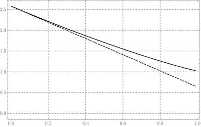
Figure 20: Left: Plots of the ratio $R(q)$, defined in (155), for $p=0.1,0.3,0.5,0.7,0.9$ (from the highest to the lowest graph), as a function of $q$. Right: Plot of $R(q)$ for $p=0.1$ and its corresponding tangent line (dashed) at $q=0$.

Using the result of Claim 40, we can now prove the following:

Corollary 41.

Let $p\leq 1/2$, $\beta_{0}$ and $\beta_{1}$ be defined according to (84) and (85), and $\mathsf{Ch}$ be the deletion channel with deletion probability $d=1-p$. Then,

$${\mathsf{Cap}}(\mathsf{Ch})\leq\frac{(1-d)\beta_{0}h(q^{\star})}{2-(3-2\beta_{1})q^{\star}},$$

where $q^{\star}\in(0,1)$ is the solution to $q^{\star}=(1-q^{\star})^{\beta_{1}-1/2}.$

Proof.

Recall that

$${\mathsf{Cap}}(\mathsf{Ch})\leq(1-d)\sup_{q\in(0,1)}C_{\mathsf{Ber}}(p,q)\leq\sup_{q\in(0,1)}\frac{\beta_{0}h(q)}{2-(3-2\beta_{1})q},$$

where the second inequality is due to Claim 40. Let $q^{\star}$ be the choice of $q$ that maximizes the right hand side of (154). The derivative of the right hand side of (154) in $q$ is equal to

$$\beta_{0}\frac{-2\log q-(1-2\beta_{1})\log(1-q)}{(2-(3-2\beta_{1})q)^{2}}.$$

By equating this derivative to zero, we see that $q^{\star}$ is the solution to $q^{\star}=(1-q^{\star})^{\beta_{1}-1/2},$ and the result follows. ∎

Table 1: Mean and normalizing constants for the distributions defined for the Poisson channel by (43) $(i=1)$ and the digamma distribution (52) $(i=2)$, for various choices of the parameter $q\in(0,1)$. For each $i\in\{1,2\}$, we have used the notation $\ell_{i}:=-\log y_{0}$ and $\mu_{i}:=\mathds{E}[Y]$ for the corresponding distribution.

$q$	$\ell_{1}$	$\mu_{1}$	$\ell_{2}$	$\mu_{2}$
0.01	0.003699	0.003719	0.002079	0.002093
0.02	0.007439	0.007523	0.004186	0.004242
0.03	0.011222	0.011413	0.006321	0.006450
0.04	0.015049	0.015393	0.008486	0.008718
0.05	0.018919	0.019464	0.010681	0.011049
0.06	0.022835	0.023631	0.012906	0.013445
0.07	0.026797	0.027897	0.015163	0.015908
0.08	0.030806	0.032264	0.017452	0.018440
0.09	0.034863	0.036737	0.019774	0.021045
0.10	0.038970	0.041319	0.022129	0.023725
0.11	0.043128	0.046014	0.024519	0.026482
0.12	0.047337	0.050825	0.026944	0.029321
0.13	0.051599	0.055758	0.029406	0.032243
0.14	0.055916	0.060816	0.031905	0.035252
0.15	0.060288	0.066004	0.034442	0.038352
0.16	0.064717	0.071327	0.037019	0.041546
0.17	0.069204	0.076789	0.039636	0.044838
0.18	0.073751	0.082397	0.042295	0.048232
0.19	0.078360	0.088156	0.044996	0.051732
0.20	0.083031	0.094071	0.047741	0.055343
0.21	0.087768	0.100150	0.050530	0.059069
0.22	0.092570	0.106397	0.053367	0.062915
0.23	0.097441	0.112821	0.056251	0.066887
0.24	0.102381	0.119428	0.059183	0.070989
0.25	0.107394	0.126226	0.062167	0.075228
0.26	0.112480	0.133223	0.065202	0.079610
0.27	0.117642	0.140427	0.068291	0.084142
0.28	0.122883	0.147848	0.071436	0.088829
0.29	0.128204	0.155495	0.074637	0.093680
0.30	0.133607	0.163377	0.077897	0.098702
0.31	0.139096	0.171506	0.081218	0.103903
0.32	0.144673	0.179893	0.084601	0.109293
0.33	0.150341	0.188549	0.088049	0.114879
0.34	0.156101	0.197487	0.091564	0.120673
0.35	0.161959	0.206722	0.095148	0.126685
0.36	0.167915	0.216266	0.098804	0.132925
0.37	0.173975	0.226135	0.102534	0.139406
0.38	0.180140	0.236346	0.106341	0.146141
0.39	0.186415	0.246916	0.110227	0.153142
0.40	0.192804	0.257863	0.114195	0.160426
0.41	0.199310	0.269207	0.118249	0.168006
0.42	0.205937	0.280969	0.122392	0.175901
0.43	0.212691	0.293172	0.126626	0.184128
0.44	0.219575	0.305840	0.130957	0.192706
0.45	0.226594	0.319000	0.135387	0.201657
0.46	0.233754	0.332679	0.139921	0.211002
0.47	0.241060	0.346908	0.144563	0.220766
0.48	0.248518	0.361719	0.149317	0.230976
0.49	0.256134	0.377147	0.154188	0.241659
0.50	0.263914	0.393231	0.159182	0.252846

$q$ $\ell_{1}$ $\mu_{1}$ $\ell_{2}$ $\mu_{2}$ $q$ $\ell_{1}$ $\mu_{1}$ $\ell_{2}$ $\mu_{2}$ 0.51 0.271866 0.410012 0.164304 0.264571 0.52 0.279996 0.427534 0.169560 0.276869 0.53 0.288312 0.445846 0.174955 0.289781 0.54 0.296823 0.465001 0.180497 0.303350 0.55 0.305537 0.485057 0.186193 0.317622 0.56 0.314465 0.506076 0.192049 0.332650 0.57 0.323615 0.528128 0.198076 0.348489 0.58 0.332999 0.551287 0.204280 0.365202 0.59 0.342629 0.575638 0.210672 0.382858 0.60 0.352517 0.601271 0.217262 0.401532 0.61 0.362676 0.628288 0.224060 0.421309 0.62 0.373121 0.656801 0.231080 0.442280 0.63 0.383869 0.686933 0.238332 0.464551 0.64 0.394935 0.718822 0.245832 0.488235 0.65 0.406338 0.752623 0.253595 0.513463 0.66 0.418099 0.788508 0.261637 0.540379 0.67 0.430240 0.826670 0.269976 0.569147 0.68 0.442784 0.867328 0.278633 0.599951 0.69 0.455759 0.910727 0.287630 0.633001 0.70 0.469192 0.957149 0.296989 0.668534 0.71 0.483117 1.006911 0.306740 0.706822 0.72 0.497569 1.060380 0.316910 0.748178 0.73 0.512586 1.117973 0.327534 0.792962 0.74 0.528214 1.180178 0.338648 0.841592 0.75 0.544500 1.247557 0.350295 0.894554 0.76 0.561501 1.320769 0.362520 0.952420 0.77 0.579279 1.400589 0.375377 1.015862 0.78 0.597905 1.487933 0.388928 1.085679 0.79 0.617460 1.583895 0.403240 1.162828 0.80 0.638037 1.689789 0.418395 1.248462 0.81 0.659744 1.807209 0.434485 1.343985 0.82 0.682705 1.938106 0.451619 1.451121 0.83 0.707068 2.084896 0.469924 1.572012 0.84 0.733006 2.250603 0.489554 1.709350 0.85 0.760730 2.439067 0.510690 1.866565 0.86 0.790489 2.655234 0.533555 2.048092 0.87 0.822593 2.905584 0.558421 2.259765 0.88 0.857427 3.198777 0.585631 2.509412 0.89 0.895475 3.546649 0.615616 2.807777 0.90 0.937364 3.965808 0.648940 3.169999 0.91 0.983921 4.480299 0.686347 3.618099 0.92 1.036269 5.126285 0.728855 4.185347 0.93 1.095987 5.960740 0.777904 4.924423 0.94 1.165396 7.078892 0.835620 5.923839 0.95 1.248104 8.652671 0.905333 7.344293 0.96 1.350183 11.027073 0.992684 9.510209 0.97 1.483060 15.010052 1.108370 13.186490 0.98 1.672514 23.035876 1.276746 20.695693 0.99 2.001316 47.343266 1.576877 43.831689 & $q$ $\ell_{1}$ $\mu_{1}$ $\ell_{2}$ $\mu_{2}$

Table 2: Capacity upper bounds for the Poisson-repeat channel with deletion probability $d=1-p=e^{-\lambda}$, as plotted in Figure 9. For each $d$, the quantity $(1-d)c_{i}$ is the capacity upper bound when method $i=1,2,3,4$ is used, and $q_{i}$ is the choice of $q$ that maximizes the function under the supremum in (75) for the chosen method. The methods are: The digamma distribution (52) for $Y$ ($i=1$, giving the strongest bounds); The elementary upper bounds of (78) on the parameters of the digamma distribution (52) $(i=2)$; The distribution defined by (43) for $Y$ $(i=3)$; The analytic upper bounds of Theorem 13 for the distribution of $Y$ defined by (43) $(i=4)$. Note that the methods $i=3$ and $4$ give trivial results for sufficiently small $d$.

$d$	$c_{1}$	$q_{1}$	$c_{2}$	$q_{2}$	$c_{3}$	$q_{3}$	$c_{4}$	$q_{4}$
0.01	0.849	0.881	0.872	0.883	1.095	0.849	1.096	0.849
0.02	0.804	0.869	0.826	0.871	1.038	0.834	1.040	0.834
0.03	0.775	0.861	0.797	0.864	1.002	0.825	1.004	0.824
0.04	0.754	0.855	0.776	0.857	0.975	0.817	0.977	0.817
0.05	0.737	0.850	0.758	0.852	0.954	0.810	0.955	0.810
0.06	0.723	0.845	0.744	0.848	0.936	0.805	0.937	0.804
0.07	0.711	0.841	0.731	0.844	0.920	0.800	0.922	0.799
0.08	0.700	0.837	0.720	0.840	0.906	0.795	0.908	0.795
0.09	0.690	0.834	0.710	0.837	0.894	0.791	0.895	0.790
0.10	0.681	0.831	0.701	0.833	0.882	0.787	0.884	0.787
0.11	0.673	0.828	0.693	0.831	0.872	0.783	0.874	0.783
0.12	0.666	0.825	0.685	0.828	0.863	0.780	0.864	0.779
0.13	0.659	0.822	0.678	0.825	0.854	0.776	0.855	0.776
0.14	0.652	0.820	0.672	0.823	0.845	0.773	0.847	0.773
0.15	0.646	0.818	0.665	0.820	0.837	0.770	0.839	0.770
0.16	0.640	0.815	0.660	0.818	0.830	0.768	0.832	0.767
0.17	0.635	0.813	0.654	0.816	0.823	0.765	0.825	0.765
0.18	0.630	0.811	0.649	0.814	0.817	0.762	0.818	0.762
0.19	0.625	0.809	0.644	0.812	0.810	0.760	0.812	0.760
0.20	0.620	0.807	0.639	0.810	0.804	0.757	0.806	0.757
0.21	0.616	0.805	0.634	0.808	0.798	0.755	0.800	0.755
0.22	0.612	0.803	0.630	0.806	0.793	0.753	0.795	0.753
0.23	0.607	0.801	0.626	0.804	0.788	0.751	0.789	0.750
0.24	0.603	0.800	0.622	0.802	0.783	0.748	0.784	0.748
0.25	0.600	0.798	0.618	0.801	0.778	0.746	0.779	0.746
0.26	0.596	0.796	0.614	0.799	0.773	0.744	0.774	0.744
0.27	0.592	0.795	0.611	0.798	0.768	0.742	0.770	0.742
0.28	0.589	0.793	0.607	0.796	0.764	0.741	0.765	0.740
0.29	0.586	0.792	0.604	0.794	0.760	0.739	0.761	0.738
0.30	0.583	0.790	0.600	0.793	0.756	0.737	0.757	0.737
0.31	0.579	0.789	0.597	0.791	0.751	0.735	0.753	0.735
0.32	0.576	0.787	0.594	0.790	0.748	0.733	0.749	0.733
0.33	0.573	0.786	0.591	0.789	0.744	0.732	0.745	0.731
0.34	0.571	0.784	0.588	0.787	0.740	0.730	0.742	0.730
0.35	0.568	0.783	0.585	0.786	0.736	0.728	0.738	0.728
0.36	0.565	0.782	0.583	0.785	0.733	0.727	0.734	0.727
0.37	0.562	0.780	0.580	0.783	0.730	0.725	0.731	0.725
0.38	0.560	0.779	0.577	0.782	0.726	0.724	0.728	0.723
0.39	0.557	0.778	0.575	0.781	0.723	0.722	0.724	0.722
0.40	0.555	0.777	0.572	0.780	0.720	0.721	0.721	0.720
0.41	0.553	0.775	0.570	0.778	0.717	0.719	0.718	0.719
0.42	0.550	0.774	0.567	0.777	0.714	0.718	0.715	0.718
0.43	0.548	0.773	0.565	0.776	0.711	0.716	0.712	0.716
0.44	0.546	0.772	0.563	0.775	0.708	0.715	0.709	0.715
0.45	0.543	0.771	0.560	0.774	0.705	0.714	0.706	0.713
0.46	0.541	0.770	0.558	0.773	0.702	0.712	0.704	0.712
0.47	0.539	0.769	0.556	0.771	0.699	0.711	0.701	0.711
0.48	0.537	0.767	0.554	0.770	0.697	0.710	0.698	0.709
0.49	0.535	0.766	0.552	0.769	0.694	0.708	0.696	0.708
0.50	0.533	0.765	0.550	0.768	0.691	0.707	0.693	0.707

$d$ $c_{1}$ $q_{1}$ $c_{2}$ $q_{2}$ $c_{3}$ $q_{3}$ $c_{4}$ $q_{4}$ $d$ $c_{1}$ $q_{1}$ $c_{2}$ $q_{2}$ $c_{3}$ $q_{3}$ $c_{4}$ $q_{4}$ 0.51 0.531 0.764 0.548 0.767 0.689 0.706 0.690 0.706 0.52 0.529 0.763 0.546 0.766 0.686 0.705 0.688 0.704 0.53 0.527 0.762 0.544 0.765 0.684 0.703 0.685 0.703 0.54 0.526 0.761 0.542 0.764 0.682 0.702 0.683 0.702 0.55 0.524 0.760 0.540 0.763 0.679 0.701 0.681 0.701 0.56 0.522 0.759 0.538 0.762 0.677 0.700 0.678 0.700 0.57 0.520 0.758 0.537 0.761 0.675 0.699 0.676 0.698 0.58 0.519 0.757 0.535 0.760 0.672 0.697 0.674 0.697 0.59 0.517 0.756 0.533 0.759 0.670 0.696 0.672 0.696 0.60 0.515 0.755 0.531 0.758 0.668 0.695 0.669 0.695 0.61 0.513 0.754 0.530 0.757 0.666 0.694 0.667 0.694 0.62 0.512 0.754 0.528 0.757 0.664 0.693 0.665 0.693 0.63 0.510 0.753 0.526 0.756 0.662 0.692 0.663 0.692 0.64 0.509 0.752 0.525 0.755 0.660 0.691 0.661 0.691 0.65 0.507 0.751 0.523 0.754 0.658 0.690 0.659 0.690 0.66 0.506 0.750 0.522 0.753 0.656 0.689 0.657 0.689 0.67 0.504 0.749 0.520 0.752 0.654 0.688 0.655 0.688 0.68 0.503 0.748 0.519 0.751 0.652 0.687 0.653 0.686 0.69 0.501 0.747 0.517 0.750 0.650 0.686 0.651 0.685 0.70 0.500 0.747 0.516 0.750 0.648 0.685 0.649 0.684 0.71 0.498 0.746 0.514 0.749 0.646 0.684 0.648 0.683 0.72 0.497 0.745 0.513 0.748 0.644 0.683 0.646 0.682 0.73 0.496 0.744 0.511 0.747 0.642 0.682 0.644 0.682 0.74 0.494 0.743 0.510 0.746 0.641 0.681 0.642 0.681 0.75 0.493 0.742 0.509 0.745 0.639 0.680 0.640 0.680 0.76 0.492 0.742 0.507 0.745 0.637 0.679 0.639 0.679 0.77 0.490 0.741 0.506 0.744 0.635 0.678 0.637 0.678 0.78 0.489 0.740 0.505 0.743 0.634 0.677 0.635 0.677 0.79 0.488 0.739 0.503 0.742 0.632 0.676 0.634 0.676 0.80 0.486 0.738 0.502 0.742 0.630 0.675 0.632 0.675 0.81 0.485 0.738 0.501 0.741 0.629 0.674 0.630 0.674 0.82 0.484 0.737 0.499 0.740 0.627 0.673 0.629 0.673 0.83 0.483 0.736 0.498 0.739 0.626 0.673 0.627 0.672 0.84 0.481 0.735 0.497 0.739 0.624 0.672 0.626 0.671 0.85 0.480 0.735 0.496 0.738 0.622 0.671 0.624 0.671 0.86 0.479 0.734 0.495 0.737 0.621 0.670 0.622 0.670 0.87 0.478 0.733 0.493 0.736 0.619 0.669 0.621 0.669 0.88 0.477 0.733 0.492 0.736 0.618 0.668 0.619 0.668 0.89 0.476 0.732 0.491 0.735 0.616 0.667 0.618 0.667 0.90 0.475 0.731 0.490 0.734 0.615 0.667 0.616 0.666 0.91 0.473 0.730 0.489 0.733 0.614 0.666 0.615 0.665 0.92 0.472 0.730 0.488 0.733 0.612 0.665 0.614 0.665 0.93 0.471 0.729 0.486 0.732 0.611 0.664 0.612 0.664 0.94 0.470 0.728 0.485 0.731 0.609 0.663 0.611 0.663 0.95 0.469 0.728 0.484 0.731 0.608 0.662 0.609 0.662 0.96 0.468 0.727 0.483 0.730 0.606 0.662 0.608 0.661 0.97 0.467 0.726 0.482 0.729 0.605 0.661 0.607 0.661 0.98 0.466 0.726 0.481 0.729 0.604 0.660 0.605 0.660 0.99 0.465 0.725 0.480 0.728 0.602 0.659 0.604 0.659 & $d$ $c_{1}$ $q_{1}$ $c_{2}$ $q_{2}$ $c_{3}$ $q_{3}$ $c_{4}$ $q_{4}$

Table 3: Capacity upper bounds for the deletion channel with deletion probability $d$, as plotted in Figure 16. For each $d$, the quantity $(1-d)c_{i}$ is the capacity upper bound when method $i=1,2,3,4$ is used, and $q_{i}$ is the choice of $q$ that maximizes the function $C_{\mathsf{Ber}}(1-d,q)$ under the supremum in (134) for the chosen method. The methods are: Theorem 34 (the truncated distribution) for the distribution of $Y$ ($i=1$, giving the strongest bounds); Theorem 26 (inverse binomial) for the distribution of $Y$ ($i=2$); Analytic upper bounds of Theorem 24 ($i=3$); The elementary upper bounds of Corollary 22 ($i=4$). Note that the analytic upper bound estimates ($i=3,4$) give trivial results for sufficiently small $d$.

$d$	$c_{1}$	$q_{1}$	$c_{2}$	$q_{2}$	$c_{3}$	$q_{3}$	$c_{4}$	$q_{4}$
0.01	0.965	0.511	0.971	0.509	1.184	0.526	3.667	0.630
0.02	0.941	0.520	0.952	0.516	1.137	0.525	2.611	0.614
0.03	0.920	0.528	0.937	0.522	1.100	0.526	2.146	0.605
0.04	0.902	0.535	0.923	0.527	1.069	0.529	1.872	0.599
0.05	0.885	0.541	0.911	0.531	1.043	0.532	1.687	0.595
0.06	0.869	0.547	0.900	0.535	1.020	0.534	1.552	0.593
0.07	0.854	0.552	0.890	0.539	1.000	0.538	1.448	0.591
0.08	0.840	0.558	0.881	0.542	0.982	0.541	1.365	0.590
0.09	0.827	0.563	0.872	0.546	0.966	0.544	1.297	0.589
0.10	0.815	0.568	0.864	0.549	0.951	0.547	1.240	0.588
0.11	0.803	0.573	0.856	0.552	0.937	0.549	1.191	0.588
0.12	0.791	0.577	0.849	0.555	0.924	0.552	1.149	0.588
0.13	0.781	0.581	0.842	0.557	0.913	0.555	1.112	0.588
0.14	0.770	0.586	0.835	0.560	0.902	0.558	1.079	0.588
0.15	0.760	0.590	0.829	0.562	0.891	0.560	1.050	0.588
0.16	0.750	0.594	0.823	0.565	0.882	0.563	1.024	0.589
0.17	0.741	0.598	0.817	0.567	0.872	0.565	1.000	0.589
0.18	0.732	0.601	0.811	0.569	0.864	0.567	0.978	0.590
0.19	0.723	0.605	0.806	0.571	0.856	0.570	0.958	0.591
0.20	0.714	0.609	0.800	0.574	0.848	0.572	0.940	0.591
0.21	0.706	0.612	0.795	0.576	0.840	0.574	0.923	0.592
0.22	0.698	0.616	0.790	0.577	0.833	0.576	0.908	0.593
0.23	0.690	0.619	0.786	0.579	0.827	0.578	0.893	0.594
0.24	0.683	0.622	0.781	0.581	0.820	0.580	0.880	0.594
0.25	0.676	0.625	0.777	0.583	0.814	0.582	0.867	0.595
0.26	0.669	0.628	0.772	0.585	0.808	0.584	0.855	0.596
0.27	0.662	0.631	0.768	0.586	0.802	0.585	0.844	0.597
0.28	0.655	0.634	0.764	0.588	0.797	0.587	0.834	0.598
0.29	0.649	0.637	0.760	0.590	0.791	0.589	0.824	0.599
0.30	0.643	0.640	0.756	0.591	0.786	0.591	0.814	0.600
0.31	0.636	0.643	0.752	0.593	0.781	0.592	0.805	0.601
0.32	0.631	0.645	0.749	0.594	0.776	0.594	0.797	0.601
0.33	0.625	0.648	0.745	0.596	0.772	0.595	0.789	0.602
0.34	0.619	0.650	0.741	0.597	0.767	0.597	0.781	0.603
0.35	0.614	0.653	0.738	0.599	0.763	0.598	0.774	0.604
0.36	0.609	0.655	0.735	0.600	0.758	0.600	0.767	0.605
0.37	0.604	0.657	0.731	0.602	0.754	0.601	0.760	0.606
0.38	0.599	0.660	0.728	0.603	0.750	0.603	0.754	0.607
0.39	0.594	0.662	0.725	0.604	0.746	0.604	0.748	0.608
0.40	0.590	0.664	0.722	0.606	0.743	0.605	0.742	0.609
0.41	0.585	0.666	0.719	0.607	0.739	0.607	0.736	0.610
0.42	0.581	0.668	0.716	0.608	0.735	0.608	0.731	0.610
0.43	0.577	0.670	0.713	0.609	0.732	0.609	0.726	0.611
0.44	0.573	0.672	0.710	0.611	0.728	0.610	0.720	0.612
0.45	0.569	0.673	0.707	0.612	0.725	0.612	0.716	0.613
0.46	0.565	0.675	0.704	0.613	0.722	0.613	0.711	0.614
0.47	0.562	0.677	0.702	0.614	0.719	0.614	0.706	0.615
0.48	0.558	0.678	0.699	0.615	0.715	0.615	0.702	0.616
0.49	0.555	0.680	0.696	0.616	0.712	0.616	0.698	0.617
0.50	0.552	0.681	0.694	0.618	0.709	0.617	0.694	0.618

$d$ $c_{1}$ $q_{1}$ $c_{2}$ $q_{2}$ $c_{3}$ $q_{3}$ $c_{4}$ $q_{4}$ $d$ $c_{1}$ $q_{1}$ $c_{2}$ $q_{2}$ $c_{3}$ $q_{3}$ $c_{4}$ $q_{4}$ 0.51 0.549 0.683 0.691 0.619 0.707 0.619 0.692 0.619 0.52 0.546 0.684 0.689 0.620 0.704 0.620 0.691 0.620 0.53 0.544 0.685 0.686 0.621 0.701 0.621 0.690 0.622 0.54 0.541 0.687 0.684 0.622 0.698 0.622 0.688 0.623 0.55 0.538 0.688 0.681 0.623 0.695 0.623 0.687 0.624 0.56 0.536 0.689 0.679 0.624 0.693 0.624 0.685 0.626 0.57 0.533 0.690 0.677 0.625 0.690 0.625 0.684 0.627 0.58 0.531 0.691 0.675 0.626 0.688 0.626 0.682 0.628 0.59 0.529 0.692 0.672 0.627 0.685 0.627 0.681 0.629 0.60 0.526 0.694 0.670 0.628 0.683 0.628 0.679 0.630 0.61 0.524 0.695 0.668 0.629 0.680 0.628 0.678 0.632 0.62 0.522 0.696 0.666 0.630 0.678 0.629 0.676 0.633 0.63 0.520 0.697 0.664 0.631 0.676 0.630 0.675 0.634 0.64 0.518 0.698 0.662 0.631 0.674 0.631 0.673 0.635 0.65 0.516 0.699 0.659 0.632 0.671 0.632 0.672 0.636 0.66 0.514 0.700 0.657 0.633 0.669 0.633 0.670 0.637 0.67 0.512 0.701 0.655 0.634 0.667 0.634 0.669 0.638 0.68 0.510 0.701 0.653 0.635 0.665 0.635 0.667 0.639 0.69 0.508 0.702 0.652 0.636 0.663 0.635 0.665 0.640 0.70 0.506 0.703 0.650 0.637 0.661 0.636 0.664 0.641 0.71 0.505 0.704 0.648 0.638 0.659 0.637 0.662 0.642 0.72 0.503 0.705 0.646 0.638 0.657 0.638 0.661 0.643 0.73 0.501 0.706 0.644 0.639 0.655 0.639 0.659 0.644 0.74 0.499 0.707 0.642 0.640 0.653 0.639 0.658 0.645 0.75 0.498 0.707 0.640 0.641 0.651 0.640 0.656 0.646 0.76 0.496 0.708 0.639 0.642 0.649 0.641 0.655 0.646 0.77 0.494 0.709 0.637 0.642 0.647 0.642 0.653 0.647 0.78 0.493 0.710 0.635 0.643 0.645 0.643 0.652 0.648 0.79 0.491 0.711 0.633 0.644 0.644 0.643 0.650 0.649 0.80 0.490 0.711 0.632 0.645 0.642 0.644 0.649 0.650 0.81 0.488 0.712 0.630 0.645 0.640 0.645 0.647 0.651 0.82 0.487 0.713 0.628 0.646 0.638 0.645 0.646 0.651 0.83 0.485 0.714 0.627 0.647 0.637 0.646 0.644 0.652 0.84 0.484 0.714 0.625 0.648 0.635 0.647 0.643 0.653 0.85 0.483 0.715 0.623 0.648 0.633 0.647 0.641 0.654 0.86 0.481 0.716 0.622 0.649 0.632 0.648 0.640 0.654 0.87 0.480 0.716 0.620 0.650 0.630 0.649 0.638 0.655 0.88 0.479 0.717 0.619 0.651 0.629 0.649 0.637 0.656 0.89 0.477 0.718 0.617 0.651 0.627 0.650 0.635 0.657 0.90 0.476 0.718 0.616 0.652 0.626 0.651 0.634 0.657 0.91 0.475 0.719 0.614 0.653 0.624 0.651 0.632 0.658 0.92 0.473 0.720 0.613 0.653 0.622 0.652 0.631 0.659 0.93 0.472 0.720 0.611 0.654 0.621 0.653 0.629 0.659 0.94 0.471 0.721 0.610 0.655 0.620 0.653 0.628 0.660 0.95 0.470 0.721 0.608 0.655 0.618 0.654 0.626 0.661 0.96 0.469 0.722 0.607 0.656 0.617 0.655 0.625 0.661 0.97 0.467 0.723 0.605 0.657 0.615 0.655 0.623 0.662 0.98 0.466 0.723 0.604 0.657 0.614 0.656 0.622 0.663 0.99 0.465 0.724 0.602 0.658 0.612 0.656 0.621 0.663 & $d$ $c_{1}$ $q_{1}$ $c_{2}$ $q_{2}$ $c_{3}$ $q_{3}$ $c_{4}$ $q_{4}$