Open system model for quantum dynamical maps with classical noise and corresponding master equations

Abstract

We show how random unitary dynamics arise from the coupling of an open quantum system to a static environment. Subsequently, we derive a master equation for the reduced system random unitary dynamics and study three specific cases: commuting system and interaction Hamiltonians, the short-time limit, and the Markov approximation.

In information theory, the dynamics of quantum systems subject solely to classical uncertainty can be modelled by random mixtures of unitary dynamics, or random unitary maps Bengtsson and Życzkowski (2006),

$$\Lambda[\hat{\rho}]=\sum_{\lambda}p_{\lambda}W_{\lambda}\hat{\rho}W_{\lambda}^{\dagger},$$ (1)

which are convex combinations of unitary Kraus operators $W_{\lambda}$ weighted with normalized probabilities $p_{\lambda}$, $\sum_{\lambda}p_{\lambda}=1$, $p_{\lambda}\in[0,1]$.

On the one hand, the Kraus form (1) has proven to be a powerful tool in derivations of general mathematical relations characterizing the dynamics of quantum systems subject to classical uncertainty Gregoratti and Werner (2003); Audenaert and Scheel (2008); Buscemi (2006); Emerson et al. (2005); Rosgen (2008). Moreover, random unitary maps have been used to study generic properties of quantum systems, such as Markovianity Chruściński and Wudarski (2015). However, the abstract formulation in terms of Kraus operators does not provide a direct physical description of quantum dynamics in terms of experimentally realizable Hamiltonians. Therefore, the experimental implementation of random unitary maps, e.g., a mixture of Pauli channels that are easily studied on a mathematical level Chruściński and Wudarski (2013), may require complicated experimental setups Liu et al. (2011).

On the other hand, random unitary maps based on microscopic models describing disordered systems Kropf et al. (2016); Gneiting et al. (2016) or open quantum systems Bengtsson and Życzkowski (2006); Chen et al. (2017) are physically motivated. Whereas these models, in general, give rise to mathematically rather complicated random unitary dynamics, they provide access to extensive methods developed in the theory of open quantum systems and of disordered systems to study the emerging dynamics. Among various methods, a distinguished role is played by master equations.

It was demonstrated in Kropf et al. (2016) how to derive and interpret master equations in the context of disordered systems. In this contribution, we will explore the open quantum system approach. To begin with, we show how random unitary dynamics arise from the coupling of an open system to a static environment. Subsequently, we derive the corresponding master equation in the Born approximation. We then discuss more explicitly three cases: commuting system and interaction Hamiltonians, the short-time limit and the semi-group Markov approximation. The first case leads to pure dephasing dynamics, the second one captures the generic Gaussian incoherent dynamics at times shorter than the Heisenberg time, and the third case is characterized by the free retarded Green’s function associated with the system Hamiltonian. These findings illustrate the intrinsic connection between disordered systems, open quantum systems and random unitary maps.

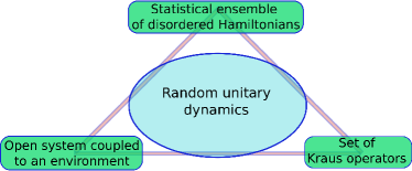
Figure 1: Random unitary dynamics can be formulated in three different frameworks. On can start from the Kraus representation, as is customary in information theory, or from an ensemble disordered time-independent Hamiltonians, as is done in disorder physics, or from the coupling of an open system to an environment, as in the theory of open quantum systems.

In the following, we consider a specific random unitary dynamics described by the following dynamical map:

$$\Lambda_{t}[\hat{\rho}]=\int d\lambda p(\lambda)U_{\lambda}(t)\hat{\rho}U_{\lambda}^{\dagger}(t),$$ (2)

where $U_{\lambda}(t)=e^{-it\hat{\textrm{H}}_{\lambda}/\hbar}$ is the unitary time-evolution operator arising from the Hamiltonian $\hat{\textrm{H}}_{\lambda}$. Note that, mathematically, it is common to consider a sum of unitary evolutions (c.f. Eq. (1)). However, for physically motivated models, it is often more natural to consider continuous combinations of unitary maps. For instance, such a situation arises when an open system is embedded in an environment with a continuous density of states. Hence, we have an integral in the right hand side of Eq. (2), with a normalized probability distribution $p(\lambda)$.

As discussed in Kropf et al. (2016), Eq. (2) can be interpreted as the ensemble-averaged dynamics of a disordered quantum system characterized by the Hamiltonian $\hat{\textrm{H}}_{\lambda}=\overline{\hat{\textrm{H}}}\leavevmode\nobreak\ +\delta\hat{\textrm{H}}_{\lambda}$, where $\delta\hat{\textrm{H}}_{\lambda}$ are random Hamiltonians distributed according to the probability distribution $p(\lambda)$ and $\overline{\hat{\textrm{H}}}\leavevmode\nobreak\ :=\int d\lambda p(\lambda)\hat{\textrm{H}}_{\lambda}$ is the average Hamiltonian. The dynamics of a single realization of the disorder is then given by $\hat{\rho}_{\lambda}(t)=U_{\lambda}(t)\hat{\rho}(0)U_{\lambda}^{\dagger}(t)$, with $U_{\lambda}(t)=e^{-it(\overline{\hat{\textrm{H}}}\leavevmode\nobreak\ +\delta\hat{\textrm{H}}_{\lambda})/\hbar}$. Correspondingly, the ensemble-averaged dynamics is obtained as $\overline{\hat{\rho}}(t):=\int d\lambda p(\lambda)\rho_{\lambda}(t)=\Lambda_{t}[\hat{\rho}(0)]$, which is a random unitary channel in the form of Eq. (2). The significance of this result stems from the fact that many quantum transport and/or interaction phenomena in complex systems can effectively be described using models of disorder. Relevant examples include the electronic transport in wires with impurities (Anderson model) Anderson (1958), the propagation of entangled photons across atmospheric turbulence Roux (2014), the exciton transport in molecular complexes Lee et al. (2015), and the inhomogeneous broadening of spectral line widths Slichter (1990).

Alternatively, as we show in the following, one can also conceive the dynamics (2) as arising from the coupling of an open quantum system to a static environment. The open system and its environment are characterized by the total Hamiltonian $\hat{\textrm{H}}^{T}=\hat{\textrm{H}}^{S}+\hat{\textrm{H}}^{\textrm{SE}}+\hat{\textrm{H}}^{E}$, where $\hat{\textrm{H}}^{S}$, $\hat{\textrm{H}}^{\textrm{SE}}$ and $\hat{\textrm{H}}^{E}$ are the Hamiltonians of the open system, the interaction and the environment, respectively. We assume an initial product (uncorrelated) state, $\hat{\rho}_{0}=\hat{\rho}_{0}^{S}\otimes\hat{\rho}_{0}^{E}$, of the system and environment. Furthermore, we assume that the environment part $\hat{\rho}_{0}^{E}$ is a stationary state of $\hat{\textrm{H}}^{E}$:

$$\hat{\rho}_{0}=\hat{\rho}_{0}^{S}\otimes\int d\lambda\,p(\lambda)\left|\lambda\rangle\langle\lambda\right|,$$ (3)

with the (orthonormal) eigenstates $\mathinner{|{\lambda}\rangle}$ of $\hat{\textrm{H}}^{E}$, and the normalized probability density $p(\lambda)$, $\int d\lambda p(\lambda)=1$.

In order to generate random unitary dynamics, we further assume that the state of the environment is time-independent. In other words, we impose the Born approximation, $\hat{\rho}(t)\approx\hat{\rho}^{S}(t)\otimes\hat{\rho}^{E}$, to hold at arbitrary times. This can be achieved by demanding

$$[\hat{\textrm{H}}^{E},\hat{\textrm{H}}^{\textrm{SE}}]=0.$$ (4)

In this case, $\hat{\textrm{H}}^{E}$ and $\hat{\textrm{H}}^{\textrm{SE}}$ share a common eigenbasis and, thus, we can parametrize the interaction Hamiltonian as

$$\hat{\textrm{H}}^{\textrm{SE}}=\int d\lambda\,\hat{\textrm{H}}_{\lambda}\otimes\left|\lambda\rangle\langle\lambda\right|.$$ (5)

The simplest example of an interaction Hamiltonian in the form of Eq. (5) is $\hat{\textrm{H}}^{\textrm{SE}}=\hat{\textrm{H}}^{A}\otimes\hat{\textrm{H}}^{B}$. Indeed, if we expand $\hat{\textrm{H}}^{B}$ in its eigenbasis $\mathinner{|{\lambda}\rangle}$ (with eigenvalues $E_{\lambda}^{B}$) we obtain $\hat{\textrm{H}}^{\textrm{SE}}=\int_{\lambda}E^{B}_{\lambda}\hat{\textrm{H}}^{A}\otimes\left|\lambda\rangle\langle\lambda\right|$. Defining $\hat{\textrm{H}}_{\lambda}\equiv E_{\lambda}\hat{\textrm{H}}^{A}$ then yields Eq. (5).

Given the initial state (3) and condition (4), the Hamiltonian of the environment plays no role in the dynamics and, thus, we can restrict our further analysis to $\hat{\textrm{H}}=\hat{\textrm{H}}^{S}+\hat{\textrm{H}}^{\textrm{SE}}$. This Hamiltonian has a block diagonal structure,

$$\hat{\textrm{H}}=\begin{pmatrix}\hat{\textrm{H}}^{S}+\hat{\textrm{H}}_{1}&\leavevmode\nobreak\ &\leavevmode\nobreak\ &\leavevmode\nobreak\ \\ \leavevmode\nobreak\ &\hat{\textrm{H}}^{S}+\hat{\textrm{H}}_{2}&\leavevmode\nobreak\ &\leavevmode\nobreak\ \\ \leavevmode\nobreak\ &\leavevmode\nobreak\ &\hat{\textrm{H}}^{S}+\hat{\textrm{H}}_{3}&\leavevmode\nobreak\ \\ \leavevmode\nobreak\ &\leavevmode\nobreak\ &\leavevmode\nobreak\ &\ldots\end{pmatrix},$$ (6)

where each block corresponds to one realisation of the random unitary channel. It is useful to include the average Hamiltonian, $\overline{\hat{\textrm{H}}}\leavevmode\nobreak\ =\int_{\lambda}p(\lambda)\hat{\textrm{H}}_{\lambda}$, into the definition of the system Hamiltonian:

$$\hat{\textrm{H}}^{S}\rightarrow\hat{\textrm{H}}^{S}+\overline{\hat{\textrm{H}}}\leavevmode\nobreak\ \;\;,\;\;\hat{\textrm{H}}_{\lambda}\rightarrow\hat{\textrm{H}}_{\lambda}-\overline{\hat{\textrm{H}}}\leavevmode\nobreak\ .$$ (7)

With this transformation, the Hamiltonian (6) remains unchanged, but the average $\int d\lambda p(\lambda)\hat{\textrm{H}}_{\lambda}=0$ now vanishes.

The dynamics of the total system is then characterized by the unitary time-evolution operator $U(t)=e^{-it\hat{\textrm{H}}/\hbar}$ and the reduced dynamics of the system is obtained by tracing out the degrees of freedom of the environment, $\hat{\rho}^{S}(t)=\text{Tr}_{E}\left[\hat{\rho}(t)\right]=\text{Tr}_{E}\left[U(t)\hat{\rho}_{0}U^{\dagger}(t)\right]$. This trace is conveniently evaluated in the orthonormal basis $\left\{\mathinner{|{\lambda}\rangle}\right\}$ of the environment,

$$\hat{\rho}^{S}(t) =\int d\lambda p(\lambda)e^{-it(\hat{\textrm{H}}^{S}+\hat{\textrm{H}}_{\lambda})/\hbar}\hat{\rho}_{0}^{S}e^{it(\hat{\textrm{H}}^{S}+\hat{\textrm{H}}_{\lambda})/\hbar}$$

$$=\int d\lambda p(\lambda)U_{\lambda}(t)\hat{\rho}_{0}^{S}U_{\lambda}^{\dagger}(t)=\Lambda_{t}\left[\hat{\rho}_{0}^{S}\right].$$ (8)

Note that in practice, one first computes the $\textrm{Tr}_{E}$ using a sum $\sum_{\lambda}$ instead of the integral $\int d\lambda$, and subsequently takes the continuum limit of the sum to obtain (8). According to Eq. (8), the reduced system dynamics forms a random unitary channel in the sense of Eq. (2).

Thus, we have shown how to obtain random unitary dynamics form the couplings of an open system to a static environment. We remark that the connection to disordered quantum systems is established by choosing the system Hamiltonian to be equal to the disorder average Hamiltonian $\hat{\textrm{H}}^{S}=\overline{\hat{\textrm{H}}}\leavevmode\nobreak\$, and the disorder realization Hamiltonian to be arising from the coupling to the environment, $\hat{\textrm{H}}_{\lambda}=\delta\hat{\textrm{H}}_{\lambda}$. Hence, the dynamics described by Eq. (2) can equivalently be derived from a microscopic disorder model or from a model of an open system coupled to an environment, or be postulated as a random unitary map (c.f. Fig. 1).

Further on, we exploit the open systems perspective to derive a quantum master equation for the random unitary dynamics (2). Our derivation focuses on the weak-coupling limit and is analogous to the one presented, e.g., in Breuer and Petruccione (2002).

At the outset, we transform to the interaction picture, where operators evolve in time with $\hat{\textrm{H}}^{S}$, while states with $\hat{\textrm{H}}^{\textrm{SE}}$. For clarity, we supply all interaction picture quantities with the subscript $I$. Next, it is useful to introduce the unitary time evolution operator, $\hat{U}_{I}=\hat{U}^{\dagger}_{0}(t)\hat{U}(t)$, where $\hat{U}_{0}(t)=e^{-it\hat{\textrm{H}}^{S}/\hbar}\otimes\mathbb{1}$ and $\hat{U}(t)$ is defined above after Eq. (7). Then, the state and the Hamiltonian in the interaction picture are given by $\hat{\rho}_{I}(t)=\hat{U}^{\dagger}_{0}(t)\hat{\rho}(t)\hat{U}_{0}(t)$ and $\hat{\textrm{H}}_{I}(t)=\hat{U}_{0}^{\dagger}(t)\hat{\textrm{H}}^{\textrm{SE}}\hat{U}_{0}(t)$, respectively. Using Eq. (5), the latter Hamiltonian can be rewritten as,

$$\hat{\textrm{H}}_{I}(t) =\int d\lambda e^{-it\hat{\textrm{H}}^{S}/\hbar}\hat{\textrm{H}}_{\lambda}e^{it\hat{\textrm{H}}^{S}/\hbar}\otimes\left|\lambda\rangle\langle\lambda\right|.$$ (9)

In the interaction picture, the dynamics of a density operator obeys the von Neumann equation,

$$\frac{d}{dt}\hat{\rho}_{I}(t)=-\frac{i}{\hbar}\left[\hat{\textrm{H}}_{I}(t),\hat{\rho}_{I}(t)\right].$$ (10)

Equation (10) is a typical starting point for the microscopic derivation of a master equation describing the dynamics of the reduced system, which here subsumes the random unitary channel. We proceed by integrating both sides of Eq. (10) over time, and subsequently inserting the result for $\hat{\rho}_{I}(t)$ back into Eq. (10), to get

$$\dot{\hat{\rho}}_{I}(t) =-\frac{i}{\hbar}\left[\hat{\textrm{H}}_{I}(t),\hat{\rho}(0)\right]$$

$$-\frac{1}{\hbar^{2}}\int_{0}^{t}dt^{\prime}\left[\hat{\textrm{H}}_{I}(t),\left[\hat{\textrm{H}}_{I}(t^{\prime}),\hat{\rho}_{I}(t^{\prime})\right]\right].$$ (11)

Note that no approximation has been made so far to derive the above integral-differential equation. It can be solved iteratively, yielding an infinite series in powers of $\hat{\textrm{H}}_{I}(t)$. Instead of doing so, let us take the trace over the environment degrees of freedom ($\textrm{Tr}_{E}$) in the exact Eq. (Open system model for quantum dynamical maps with classical noise and corresponding master equations),

$$\dot{\hat{\rho}}_{I}^{S}(t)= -\frac{i}{\hbar}\int d\lambda p(\lambda)\left[\hat{U}_{0}^{S\dagger}(t)\hat{\textrm{H}}_{\lambda}\hat{U}_{0}^{S}(t),\hat{\rho}^{S}_{0}\right]$$ (12)

$$-\frac{1}{\hbar^{2}}\textrm{Tr}_{E}\left\{\int_{0}^{t}dt^{\prime}\left[\hat{\textrm{H}}_{I}(t),\left[\hat{\textrm{H}}_{I}(t^{\prime}),\hat{\rho}_{I}(t^{\prime})\right]\right]\right\},$$

with $\hat{U}^{S}_{0}(t)=e^{-it\hat{\textrm{H}}^{S}/\hbar}$ the interaction picture unitary evolution operator of the system. The first term on the right-hand side of Eq. (12) vanishes due to the transformation (7), which ensures that $\int d\lambda p(\lambda)\hat{\textrm{H}}_{\lambda}=0$. As for the second term, we recall that in the Born approximation that we are using , $\hat{\rho}(t)=\hat{\rho}^{S}(t)\otimes\hat{\rho}^{E}$. This leads to the result,

$$\hat{\rho}_{I}(t^{\prime}) =\hat{\rho}_{I}^{S}(t^{\prime})\otimes\hat{\rho}^{E}$$

$$=\hat{U}_{0}^{S\dagger}(t^{\prime})\hat{\rho}_{0}^{S}\hat{U}_{0}^{S}(t^{\prime})\otimes\int d\lambda p(\lambda)\left|\lambda\rangle\langle\lambda\right|.$$ (13)

Inserting the latter result into Eq. (12) and performing the trace over the environment, we obtain

$$\dot{\hat{\rho}}_{I}^{S}(t)=-\frac{1}{\hbar^{2}}\int_{0}^{t}dt^{\prime}\int d\lambda p(\lambda)\left[{\hat{\textrm{H}}_{\lambda}}_{I}(t),\left[{\hat{\textrm{H}}_{\lambda}}_{I}(t^{\prime}),\hat{\rho}^{S}_{I}(t^{\prime})\right]\right],$$ (14)

where $\hat{\textrm{H}}_{\lambda I}(t)=U_{0}^{\dagger}(t)\hat{\textrm{H}}_{\lambda}U_{0}(t)$.

We now make a further approximation,

$$\hat{\rho}_{I}^{S}(t^{\prime})\approx\hat{\rho}_{I}^{S}(t),$$ (15)

which renders Eq. (14) local in time. This approximation is justified in the regime of weak system-environment coupling and amounts to the truncation of the infinite series expansion by the terms that are second-order in $\hat{\textrm{H}}_{I}(t)$ Ishizaki and Tanimura (2008). In the context of disordered systems, this is equivalent to considering at most second-order correlations of the disorder potential.

Applying the approximation (15) in Eq. (14), we arrive at a Redfield master equation Breuer and Petruccione (2002); Redfield (1957) in the interaction picture,

$$\dot{\hat{\rho}}_{I}^{S}(t) =-\frac{1}{\hbar^{2}}\int_{0}^{t}dt^{\prime}\int d\lambda p(\lambda)\left[{\hat{\textrm{H}}_{\lambda}}_{I}(t),\left[{\hat{\textrm{H}}_{\lambda}}_{I}(t^{\prime}),\hat{\rho}^{S}_{I}(t)\right]\right].$$ (16)

Dropping the (now, redundant) superscript $S$ of the density matrix and reverting back to the Schrödinger picture, we obtain the master equation,

$$\dot{\hat{\rho}}(t)=- \frac{i}{\hbar}\left[\hat{\textrm{H}}^{S},\hat{\rho}(t)\right]-\frac{1}{\hbar^{2}}\int d\lambda\,p_{\lambda}\left[\hat{\textrm{H}}_{\lambda},\left[\tilde{\hat{\textrm{H}}}_{\lambda}(t),\hat{\rho}(t)\right]\right],$$ (17)

where

$$\tilde{\hat{\textrm{H}}}_{\lambda}(t) :=\int_{0}^{t}dt^{\prime}e^{-it^{\prime}\hat{\textrm{H}}^{S}/\hbar}\hat{\textrm{H}}_{\lambda}e^{it^{\prime}\hat{\textrm{H}}^{S}/\hbar}.$$ (18)

In the following, we explore the properties of Eq. (17) for three different scenarios.

a) Commuting system and interaction Hamiltonians: As a first example, let us consider a system whose Hamiltonian commutes with the interaction Hamiltonian,

$$\left[\hat{\textrm{H}}^{S},\hat{\textrm{H}}_{\lambda}\right]=0\;,\;\forall\lambda.$$ (19)

In this case, Eq. (18) is elementarily integrated to yield the relation

$$\tilde{\hat{\textrm{H}}}_{\lambda}(t)=t\hat{\textrm{H}}_{\lambda}.$$ (20)

Consequently, the master equation (17) becomes,

$$\dot{\hat{\rho}}(t)= -\frac{i}{\hbar}\left[\hat{\textrm{H}}^{S},\hat{\rho}(t)\right]-\frac{t}{\hbar^{2}}\int d\lambda p_{\lambda}\left[\hat{\textrm{H}}_{\lambda},\left[\hat{\textrm{H}}_{\lambda},\hat{\rho}(t)\right]\right].$$ (21)

Equation (21) is easily solved in the eigenbasis $\mathinner{|{n}\rangle}$ that is common to $\hat{\textrm{H}}^{S}$ and $\hat{\textrm{H}}_{\lambda}$, with the matrix elements of the density operator given by

$$\rho_{nm}(t)=\rho_{nm}(0)e^{-it(E_{n}^{S}-E_{m}^{S})/\hbar}e^{-t^{2}C_{2}(n,m)/2\hbar^{2}},$$ (22)

where

$$C_{2}(n,m)=\int d\lambda p_{\lambda}(E_{n}^{\lambda}-E_{m}^{\lambda})^{2},$$ (23)

is the two-point correlation function which has the meaning of the average square of the energy gap between levels $n$ and $m$. Equation (22) signifies pure dephasing dynamics: the diagonal elements ($n=m$) are time-independent, while the off-diagonal elements ($n\neq m$) evolve coherently with $\hat{\textrm{H}}^{S}$, and on top of that undergo a Gaussian decay with a linearly increasing in time rate $\gamma_{nm}(t)=tC_{2}(n,m)/\hbar^{2}$. As it includes all contributions from the two-point correlations, the master equation (21) is exact in the limit where the initial state distribution $p(\lambda)$ is a Gaussian. A rigorous proof thereof for finite-dimensional systems can be easily derived by adapting corollary 3.1 of Wißmann (2016).

Furthermore, taking the disorder instead of open system perspective, the condition (19) is equivalent to the requirement that the disorder affects only the eigenvalues (i.e., spectral disorder) Kropf et al. (2016). On can then show that the exact dynamics also results in pure dephasing Kropf et al. (2016), and, hence, is not a consequence of the weak-coupling approximation given by Eq. (15), but is a direct consequence of the commutation relation (19).

b) Short times: Let us now study the behaviour of $\hat{\rho}(t)$ at short times. For that purpose, we expand Eq. (18) to first order in time, which yields the same result as for condition (19), namely $\tilde{\hat{\textrm{H}}}_{\lambda}(t)=t\hat{\textrm{H}}_{\lambda}$. Hence, again, the corresponding master equation is Eq. (21). Note that, since the Hamiltonians $\hat{\textrm{H}}_{\lambda}$ for different $\lambda$ may not commute with each other, in this case the dynamics does not necessarily result in pure dephasing. Comparing the first- and second-order terms in the series expansion of the exponential in Eq. (22), the validity time $\tau$ can be estimated to be proportional to the mean level spacing of the system Hamiltonian,

$$\tau\approx\frac{\hbar}{\left<E_{m}^{S}-E_{n}^{S}\right>}.$$ (24)

This time scale is given by the energy-time uncertainty relation Le Bellac (2006), and is sometimes termed Heisenberg time (see, e.g., Wimberger (2014)).

c) Markov approximation: A common approximation in the study of open quantum systems is the semi-group Markov approximation which leads to the Gorini-Kossakowski-Sudarshan-Lindblad (GKSL) master equation Lindblad (1976); Gorini et al. (1976). To derive the latter, we begin by expanding Eq. (18) in the eigenbasis $\mathinner{|{n}\rangle}$ of the system Hamiltonian

$$\tilde{\hat{\textrm{H}}}_{\lambda}(t)= \sum_{m,n=1}^{d}\left|m\rangle\langle m\right|\hat{\textrm{H}}_{\lambda}\left|n\rangle\langle n\right|\int_{0}^{t}dt^{\prime}e^{-\frac{i}{\hbar}(t-t^{\prime})(E^{S}_{m}-E^{S}_{n})},$$ (25)

with $E^{S}_{n}$ the $n^{th}$ eigenvalue of $\hat{\textrm{H}}^{S}$ and $d={\rm dim}(\hat{\textrm{H}}^{S})$.

The semigroup Markov approximation is obtained by setting the upper integration limit of the time integral in Eq. (25) to infinity:

$$\underset{t\rightarrow\infty}{\lim}\int_{0}^{t}dt^{\prime}e^{-\frac{i}{\hbar}(t-t^{\prime})(E^{S}_{m}-E^{S}_{n})}=\underset{\epsilon\rightarrow 0}{\lim}\frac{i\hbar}{E^{S}_{n}-E^{S}_{m}+i\epsilon}=:R_{mn}.$$ (26)

We then obtain

$$\tilde{\hat{\textrm{H}}}_{\lambda}=\sum_{m,n=1}^{d}R_{mn}\langle m|\hat{\textrm{H}}_{\lambda}|n\rangle\left|m\rangle\langle n\right|.$$ (27)

The above expression (26) is the matrix element $R_{mn}=\langle m|\hat{G}_{S}(E_{n})|m\rangle$ of the free retarded resolvent operator $\hat{G}_{S}(E)=(E-\hat{\textrm{H}}^{S}+i\epsilon)^{-1}$. In other words, $R_{mn}$ is the transition amplitude from state $\mathinner{|{m}\rangle}$ to $\mathinner{|{n}\rangle}$ of a particle evolving only with the system Hamiltonian $\hat{\textrm{H}}^{S}$.

Inserting Eq. (27) into Eq. (17) yields a GKSL master equation, which is by definition time-independent. Hence, it is clear that the Markov approximation cannot be applied to the previous two examples, which are characterized by the time-dependent master equation (21). Finally, we note that when the GKLS master equation arises as a consequence of averaging over random impurities in a disordered sample, one obtains pure momentum-dephasing random unitary dynamics Müller (2009).

In this article we studied a particular class of random unitary channels and showed how to embed the latter in the framework of the theory of open quantum systems. Making use of the fact that our random unitary channels imply the Born approximation, we derived the corresponding Redfield master equation. We then studied in more detail three specific cases: commuting system and interaction Hamiltonians, the short-time approximation and the semi-group Markov approximation. We showed that in the first case, one obtains a pure dephasing master equation with rates that are linearly increasing with time. In the second case, we obtained a master equation with the same rates, but that does not invariably lead to dephasing dynamics. In the semi-group Markov approximation, the resulting GKLS master equation is characterized by the transition amplitudes generated by the system Hamiltonian.

In conclusion, the dynamics of quantum systems subject to classical uncertainty can be studied either starting from the random unitary Kraus map Eq.(1) Bengtsson and Życzkowski (2006), from an ensemble of disordered Hamiltonians Kropf et al. (2016), or, as discussed here, from a system coupled to a static environment. Each approach allows for specific computational methods and provides particular grounds for experimental implementations. We believe that these different points of view are fruitful for fostering synergies between the fields of open quantum systems, disorder physics and information theory Kropf (2017).

The authors wish to express their gratitude for discussions with Clemens Gneiting. C. K. acknowledges funding by the German National Academic Foundation.

References

- Bengtsson and Życzkowski (2006) I. Bengtsson and K. Życzkowski, Geometry of Quantum States: An Introduction to Quantum Entanglement (Cambridge University Press, 2006).
- Gregoratti and Werner (2003) M. Gregoratti and R. F. Werner, J. Mod. Opt. 50, 915 (2003).
- Audenaert and Scheel (2008) K. M. R. Audenaert and S. Scheel, New J. Phys. 10, 023011 (2008).
- Buscemi (2006) F. Buscemi, Phys. Lett. A 360, 256 (2006).
- Emerson et al. (2005) J. Emerson, R. Alicki, and K. Życzkowski, J. Opt. B 7, S347 (2005).
- Rosgen (2008) B. Rosgen, J. Math. Phys. 49, 102107 (2008).
- Chruściński and Wudarski (2015) D. Chruściński and F. A. Wudarski, Phys. Rev. A 91, 012104 (2015).
- Chruściński and Wudarski (2013) D. Chruściński and F. A. Wudarski, Phys. Lett. A 377, 1425 (2013).
- Liu et al. (2011) B.-H. Liu, L. Li, Y.-F. Huang, C.-F. Li, G.-C. Guo, E.-M. Laine, H.-P. Breuer, and J. Piilo, Nat. Phys. 7, 931 (2011).
- Kropf et al. (2016) C. M. Kropf, C. Gneiting, and A. Buchleitner, Phys. Rev. X 6, 031023 (2016).
- Gneiting et al. (2016) C. Gneiting, F. R. Anger, and A. Buchleitner, Phys. Rev. A 93, 032139 (2016).
- Chen et al. (2017) H.-B. Chen, C. Gneiting, P.-Y. Lo, Y.-N. Chen, and F. Nori, arXiv:1703.09428 (2017).
- Anderson (1958) P. W. Anderson, Phys. Rev. 109, 1492 (1958).
- Roux (2014) F. S. Roux, J. Phys. A 47, 195302 (2014).
- Lee et al. (2015) E. M. Y. Lee, W. A. Tisdale, and A. P. Willard, J. Phys. Chem. B 119, 9501 (2015).
- Slichter (1990) C. P. Slichter, Principles of Magnetic Resonance (Springer, 1990).
- Breuer and Petruccione (2002) H. P. Breuer and F. Petruccione, The Theory of Open Quantum Systems (Oxford University Press, 2002).
- Ishizaki and Tanimura (2008) A. Ishizaki and Y. Tanimura, Chem. Phys. 347, 185 (2008).
- Redfield (1957) A. G. Redfield, IBM J. RES. DEV. 1, 19 (1957).
- Wißmann (2016) S. Wißmann, Non-Markovian Quantum Probes for Complex Systems, Ph.D. thesis, Albert-Ludwigs-University, Freiburg (2016).
- Le Bellac (2006) M. Le Bellac, Quantum Physics (Cambridge University Press, Cambridge, 2006).
- Wimberger (2014) S. Wimberger, Nonlinear Dynamics and Quantum Chaos, Graduate Texts in Physics (Springer International Publishing, Cham, 2014).
- Lindblad (1976) G. Lindblad, Commun. Math. Phys. 48, 119 (1976).
- Gorini et al. (1976) V. Gorini, A. Kossakowski, and E. C. G. Sudarshan, J. Math. Phys. 17, 821 (1976).
- Müller (2009) C. A. Müller, in Entanglement and Decoherence, Lecture Notes in Physics No. 768, edited by A. Buchleitner, C. Viviescas, and M. Tiersch (Springer Berlin Heidelberg, 2009) pp. 277–314.
- Kropf (2017) C. Kropf, Effective Dynamics of Disordered Quantum Systems, Ph.D. thesis, University of Freiburg, Freiburg (2017).