The Local Dimension of Deep Manifold
Abstract
Based on our observation that there exists a dramatic drop for the singular values of the fully connected layers or a single feature map of the convolutional layer, and that the dimension of the concatenated feature vector almost equals the summation of the dimension on each feature map, we propose a singular value decomposition (SVD) based approach to estimate the dimension of the deep manifolds for a typical convolutional neural network VGG19. We choose three categories from the ImageNet, namely Persian Cat, Container Ship and Volcano, and determine the local dimension of the deep manifolds of the deep layers through the tangent space of a target image. Through several augmentation methods, we found that the Gaussian noise method is closer to the intrinsic dimension, as by adding random noise to an image we are moving in an arbitrary dimension, and when the rank of the feature matrix of the augmented images does not increase we are very close to the local dimension of the manifold. We also estimate the dimension of the deep manifold based on the tangent space for each of the maxpooling layers. Our results show that the dimensions of different categories are close to each other and decline quickly along the convolutional layers and fully connected layers. Furthermore, we show that the dimensions decline quickly inside the Conv5 layer. Our work provides new insights for the intrinsic structure of deep neural networks and helps unveiling the inner organization of the black box of deep neural networks.
1 Introduction
To have a better understanding of deep neural networks, a recent important trend is to analyze the structure of the high-dimensional feature space. Capitalizing on the manifold hypothesis (Cayton 2005; Narayanan & Mitter 2010), the distribution of the generated data is assumed to concentrate in regions of low dimensionality. In other words, it is assumed that activation vectors of deep neural networks lie on different low dimensional manifolds embedded in high dimensional feature space.
Note that the rationality of many manifold learning algorithms based on deep learning and auto-encoders is that one learns an explicit or implicit coordinate system for leading factors of variation. These factors can be thought of as concepts or abstractions that help us understand the rich variability in the data, which can explain most of the structure in the unknown data distribution. See Goodfellow et al. (2016) for more information.
The dimension estimation is crucial in determining the number of variables in a linear system, or in determining the number of degrees of freedom of a dynamic system, which may be embedded in the hidden layers of neural networks. Moreover, many algorithms in manifold learning require the intrinsic dimensionality of the data as a crucial parameter. Therefore, the problem of estimating the intrinsic dimensionality of a manifold is of great importance, and it is also a crucial start for manifold learning.
Unfortunately, the manifold of interest in AI (especially for deep neural networks), is such a rugged manifold with a great number of twists, ups and downs with strong curvature. Thus, there is a fundamental difficulty for the manifold learning, as raised in Bengio & Monperrus (2005), that is, if the manifolds are not very smooth, one may need a considerable number of training examples to cover each one of these variations, and there is no chance for us to generalize to unseen variations.
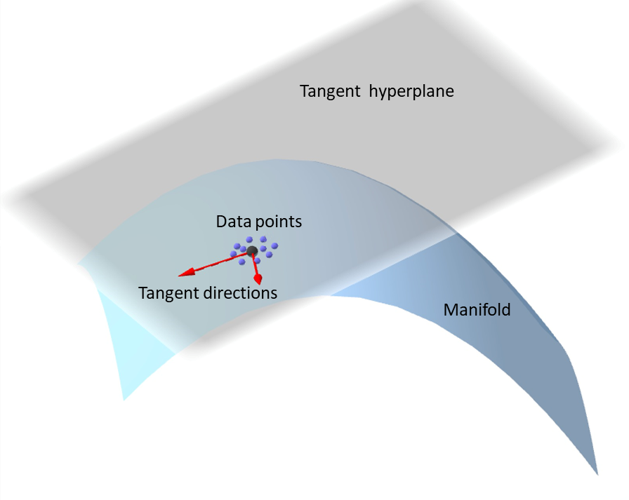
Our work is based on an important characterization of the manifold, namely, the set of its tangent hyperplanes. For a point on a -dimensional manifold, the tangent hyperplane is given by a local basis of vectors that span the local directions of variations allowed on the manifold. As illustrated in Figure 1, these local directions specify how one can change infinitesmally while staying on the manifold.
Based on above analysis, our work focuses on a thorough exploration of the local hyperplane dimension of the activation manifold in deep neural networks. Creating an artificial data cluster concentrated in regions of the local tangent hyperplane, we apply SVD to the data cluster in different layers or feature maps in neural networks. Through thorough analysis, we reach the following fascinating results.
-
•
There exists a dramatic drop for the singular values of the fully connected layers or a single feature map of the convolutional layer.
-
•
For convolutional layers, the dimension of the concatenated feature vector almost equals the summation of the dimension on each feature map.
-
•
The dimensions of different image categories are close and the dimension declines quickly along the layers.
To our knowledge this is the first thorough exploration of manifold dimension on very deep neural networks. We wish our work sheds light on new understandings and inspires further investigations on the structure of manifolds in deep neural networks.
2 Related Work
With the great success of deep learning in many applications including computer vision and machine learning, a comprehensive understanding of the essence of deep neural networks is still far from satisfactory. Related works can be classified mainly into three types. The first kind of work focuses on the difference of random networks and trained networks (Saxe et al., 2011; He et al., 2016; Rahimi & Recht, 2009). There are also works that focus on the theoretical understanding of learning (Zhang et al., 2017; Li & Yuan, 2017), while the rest focus on the inner organization or feature representations through visualization (Mahendran & Vedaldi, 2015; Dosovitskiy & Brox, 2016).
Up until now, there are only a few works in exploring the property of deep manifolds formed by activation vectors of the deep layers. In this section, we highlight the most related work for manifold learning and dimension determination.
Manifold learning has been mainly applied in unsupervised learning procedures that attempt to capture the manifolds (Van der Maaten & Hinton, 2008). It associates each of the activation nodes with a tangent plane that spans the directions of variations associated with different vectors between the target example and its neighbors. Weinberger et al. (2004) investigate how to learn a kernel matrix for high dimensional data that lies on or near a low dimensional manifold. Rifai et al. (2011) exploit a novel approach for capturing the manifold structure (high-order contractive auto-encoders) and show how it builds a topological atlas of charts, with each chart characterized by the principal singular vectors of the Jacobian of a representation mapping. Kingma et al. (2014) propose a two-dimensional representation space, a Euclidean coordinate system for Frey faces and MNIST digits, learned by a variational auto-encoder.
There are several efficient algorithms to determine the intrinsic dimension of high-dimensional data. Singular Value Decomposition (SVD), also known as Principal Component Analysis (PCA), has been discussed thoroughly in the literature Strang et al. (1993). In applications, the choice of algorithm will rely on the geometric prior of the given data and the expectation of the outcome. In addition, researchers have also proposed several improved manifold-learning algorithms considering more pre-knowledge of the dataset. For example, Little et al. (2009) estimate the intrinsic dimensionality of samples from noisy low-dimensional manifolds in high dimensions with multi-scale SVD. Levina & Bickel (2005) propose a novel method for estimating the intrinsic dimension of a dataset by applying the principle of maximum likelihood to the distances between close neighbors. Haro et al. (2008) introduce a framework for a regularized and robust estimation of non-uniform dimensionality and density for high dimensional noisy data.
To have a comprehensive understanding of the manifold structure of neural networks, it is natural to treat the activation space as a high-dimensional dataset and then characterize it by determining the dimension. This will give us a new view of the knowledge learnt from the neural network and hopefully the information hidden inside. However, to the best of our knowledge, there is nearly no related work in determining the intrinsic dimensionality of the deep manifold embedded in the neural network feature space. In the following we will give a thorough study on this topic.
3 Manifold Dimension Characterization
In this section we describe our strategy to determine the dimension of the local tangent hyperplane of the manifold, along with necessary definitions and conventions which will be used in specifying the dimension of the manifold dataset.
3.1 determine dimension by svd
It is known that if there is a set of data that can be regarded as a data point cluster and lie close to a noiseless -dimensional hyperplane, then by applying SVD, the number of non-trivial singular values will equal to — the intrinsic dimension of the data point cluster. In the context of a manifold in a deep neural network, a cluster of activation vectors pointing to a manifold embedded in feature space , can be approximated as concentrated on a -dimensional tangent hyperplane, whose dimension directly associates with the manifold.
However, the challenge here in dimension estimation is that noise everywhere are influencing the dataset making it hard to get the correct result:
-
1.
Little et al. (2009) point out that when D-dimensional noise is added to the data, we will observe :, where represents noise. The noise will introduce perturbation of the covariance matrix of the data, which will lead to the wrong result.
-
2.
Goodfellow et al. (2016) also mentioned that some factors of variation largely influence every single piece of the observed data. Thus those factors we do not care about (or simply considered as noise) may lead researchers to wrong result with high probability.
To solve the above problems, we make use of the following observations:
-
1.
By introducing representations that are expressed in terms of different, simpler representations, deep neural networks extract high-level, abstract features from the raw data, that make it successfully disentangle the factors of variation and discard the ones that we do not care about (noise), see Goodfellow et al. (2016) for more information. It turns out that the noise in feature space will be so small that we are likely to have the singular values from factors we care about significantly larger than the remaining singular values generated by noise and get the right result.
-
2.
Johnstone (2001) and many works have shown that when , the number of data points, goes to infinity, the behavior of this estimator is fairly well understood.
Based on the above analysis, we propose the following solution:
-
1.
By using a pre-trained deep neural network, after the feed-forward process, the feature vectors have little irrelevant noise remaining and preserve all useful factors of variation. So we can make sure that feature vectors lie on a noiseless manifold embedded in high dimensional feature space.
-
2.
By introducing some picture augmentation methods, we will generate considerable amount of similar pictures(also classified as the same class with high probability by deep neural network), then we will get a sufficiently large cluster of feature vectors that lie close to a local tangent -dimensional hyperplane of the noiseless manifold.
-
3.
Finally we apply the original SVD on this feature vector cluster which lies close to noiseless local tangent -dimensional hyperplane and give a precise estimation of the local dimension of the manifold.
Following paragraphs give a more formal description of our solution to computing the dimension.
Let be the set of image data points we generate, is the original image classified by the neural network as a specific class with high probability,e.g . By using augmentation methods, we generate augmented images and keep all augmented images classified to be in the same class with high probability. , .
Let be augmentation information we have introduced to the image. The can be divided into two components: some irrelevant noise() combined with useful factors of variance(), let be the underlying network feature extract function. After feed-forward process in a specific layer, feature vectors in are denoted as a matrix . For simplicity, we denote as . is the local approximate hyperplane of manifold .
In the real image space, we have . But after feed-forward process in the feature space, the noise is reduced to very small scale and we got . Therefore activation vectors are concentrated around a noiseless local tangent hyperplane of manifold .
To realize the goal of estimating local tangent of manifold given and corresponding in a specific layer, we adopt the standard approach to compute the SVD, with the singular values (denoted as ) yielding . With high probability the first singular values are significant, so that , we then take the reasonable estimation that .
3.2 estimate the manifold dimension of different layers
Fully connected layers. For fully connected layers, the size of would be . Then we apply SVD on to get its singular value array that sorted in descending order. Let denotes the i-th singular value in the array, if there exist some , where , in which is a very big number, then we claim that is an estimation of the tangent hyperplane ’s dimension, so is the estimation of the local dimension of manifold of corresponding layer and original images. If the does not exist, then the estimation of the local dimension would be up to the dimension of the whole activation space(see Section 5).
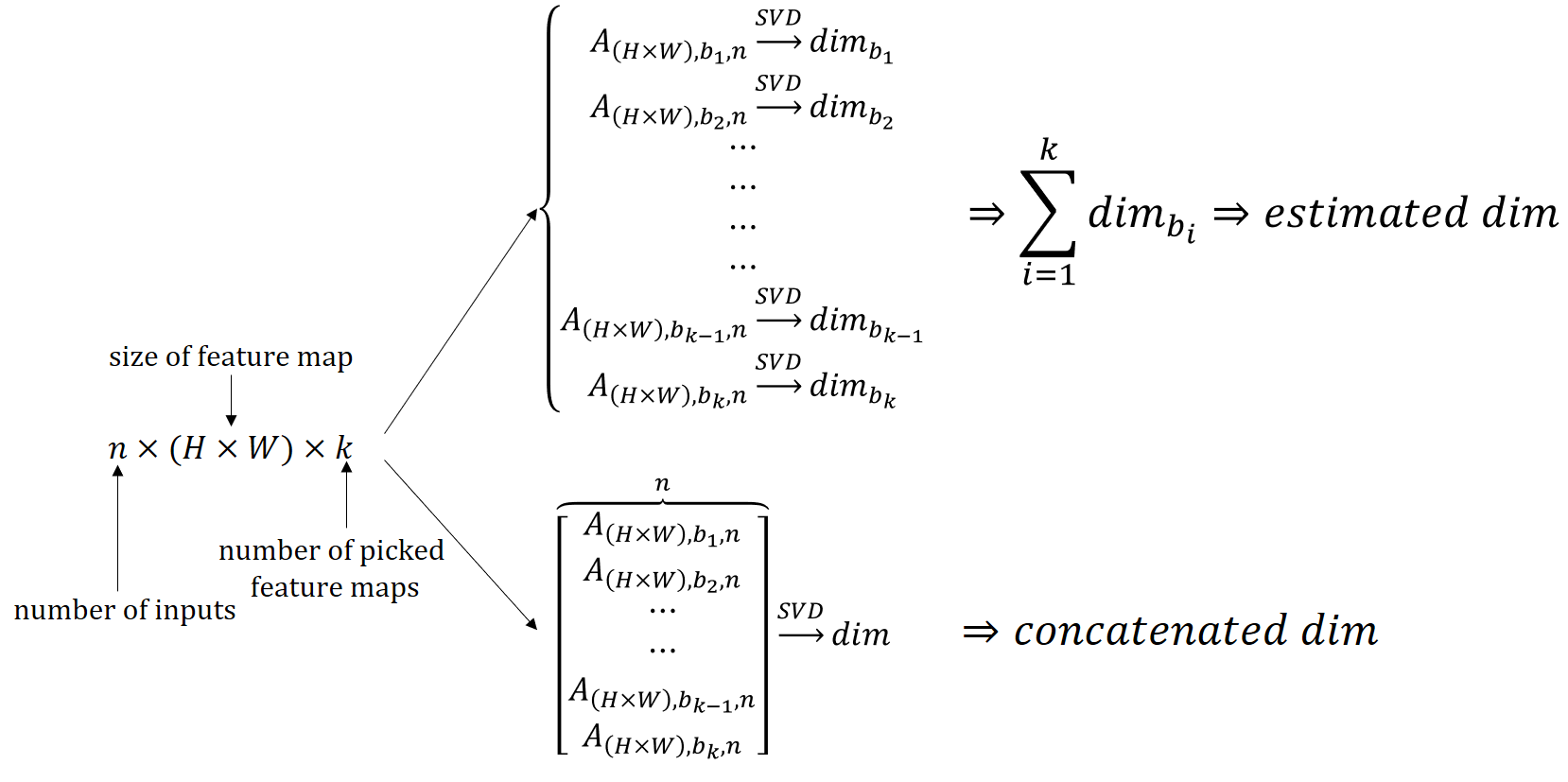
Convolutional layers. We denote as the activation space dimension of a specific layer with whose is feature map’s height, is the width of feature map , is the number of channel. For data cluster with size and the th feature map with height and width in the convolutional layer we got a corresponding matrix and calculate dimension respectively.
We define the estimated dimension by randomly picking feature maps and calculating their dimension one by one and sum the dimensions up. Concatenated dimension: concatenate the picked feature maps and calculate the concatenated matrix’s dimension. Original dimension: when we pick all the feature maps in a layer and calculate the concatenated dimension, this concatenated dimension is defined as the original dimension. Figure 2 is a illustration of these concepts.
We should note that fully-connected layers’ are 1 (), so in fully-connected layer, the estimated dimension = concatenated dimension = original dimension. We will refer to either of it for the same meaning. When we refer to a layer’s estimated dimension (or estimated dimension of a layer), we mean we choose all feature maps and do calculation ().
4 Experimental Setup
Network. VGG19 was proposed by Simonyan & Zisserman (2014), it was proved to have excellent performance in the ILSVRC competition, whose pre-trained model are still wildly used in many areas. In this paper, we use pre-trained VGG19 model to conduct our experiment, and give every layer a unique name so that they can be referred to directly. Table 2 in Appendix gives the name of every layer and its corresponding activation space dimension.
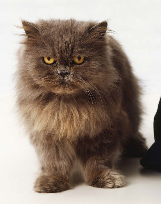
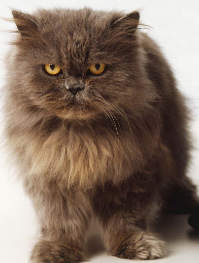
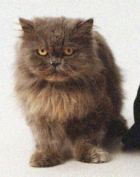
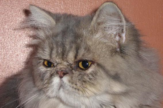
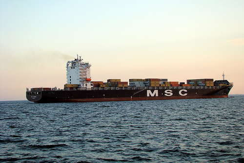
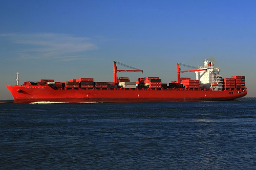
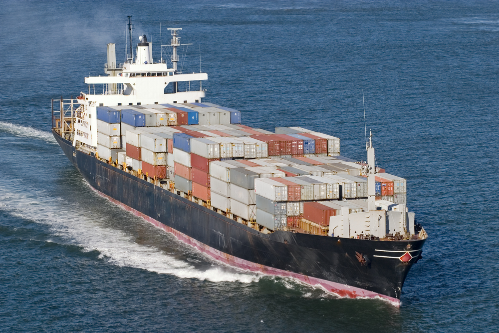
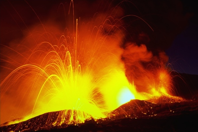
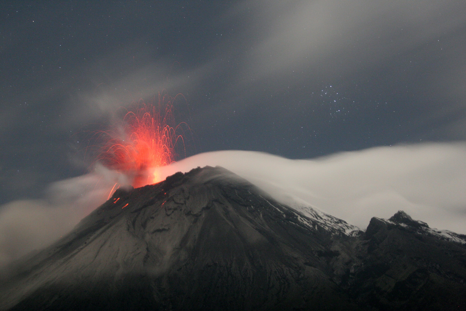
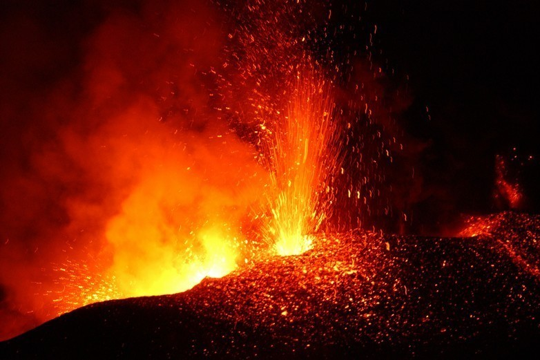
Image augmentation. We choose three categories in ImageNet dataset: Persian Cat (n02123394), Container Ship (n03095699) and Volcano (n09472597) (See Figure 11 in Appendix). Then for each category, we select three typical images with high probability as the original images, because the network firmly believe that they are in the category, their activation vectors can be considered as a data point on the same manifold representing Persian Cat.
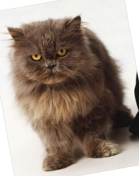
We use three augmentation methods to generate similar images which form a data point cluster, they are: 1) Cropping: randomly cut out a strip of few pixels from every edge; 2) Gaussian noise: add Gaussian noise (mean = 0.0, var = 0.01) to every single pixel; 3) Rotation: rotate the image by a random degree in . The exaggerated output images of these three methods are shown in Figure 3.
As these augmentation methods only apply small changes on the original image (also keep high probability ), activation vectors will concentrate around the activation vector of , which can be considered near a local tangent hyperplane of the manifold .
5 Supported Experiments
We have tried three Persian cat images, the dimension is within a small range. For other categories, we also tried three high-probability images for ship and three high-probability images for volcano. The dimension of vocano is slightly higher than that of cat, and the dimension of cat is slightly higher than ship for the same layer. All the three category show the same trend on dimension through the layers. Therefore, we will show the details mainly on a typical Persian cat as shown in Figure 3 (a).
Estimated dimension for a fully connected layer or a single feature map. We apply SVD on in fully connected layers and then plot the singular values in log10 scale ( Figure 5). If we specify a certain layer, we can find dramatic drop at for all the three augmenting methods: . So we can claim that for the local tangent hyperplane on manifold , the dimension is with high probability as long as we use enough samples (See Section 3.1). This “dramatic drop” also appears for a single feature map. The only exception is on the fc8 layer, there is no “dramatic drop”, inferring that the hyperplane spans the whole activation space. in fc8.
Rule 1. The estimated dimension of the local tangent hyperplane of the manifold for a fully connected layer or a single feature map can be determined by a dramatic drop along the singular values.
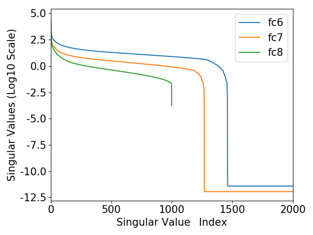
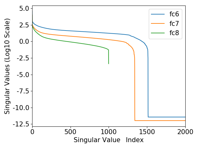
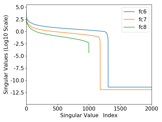
fc6 and fc7 have dramatic drops.
= concatenated dimension.
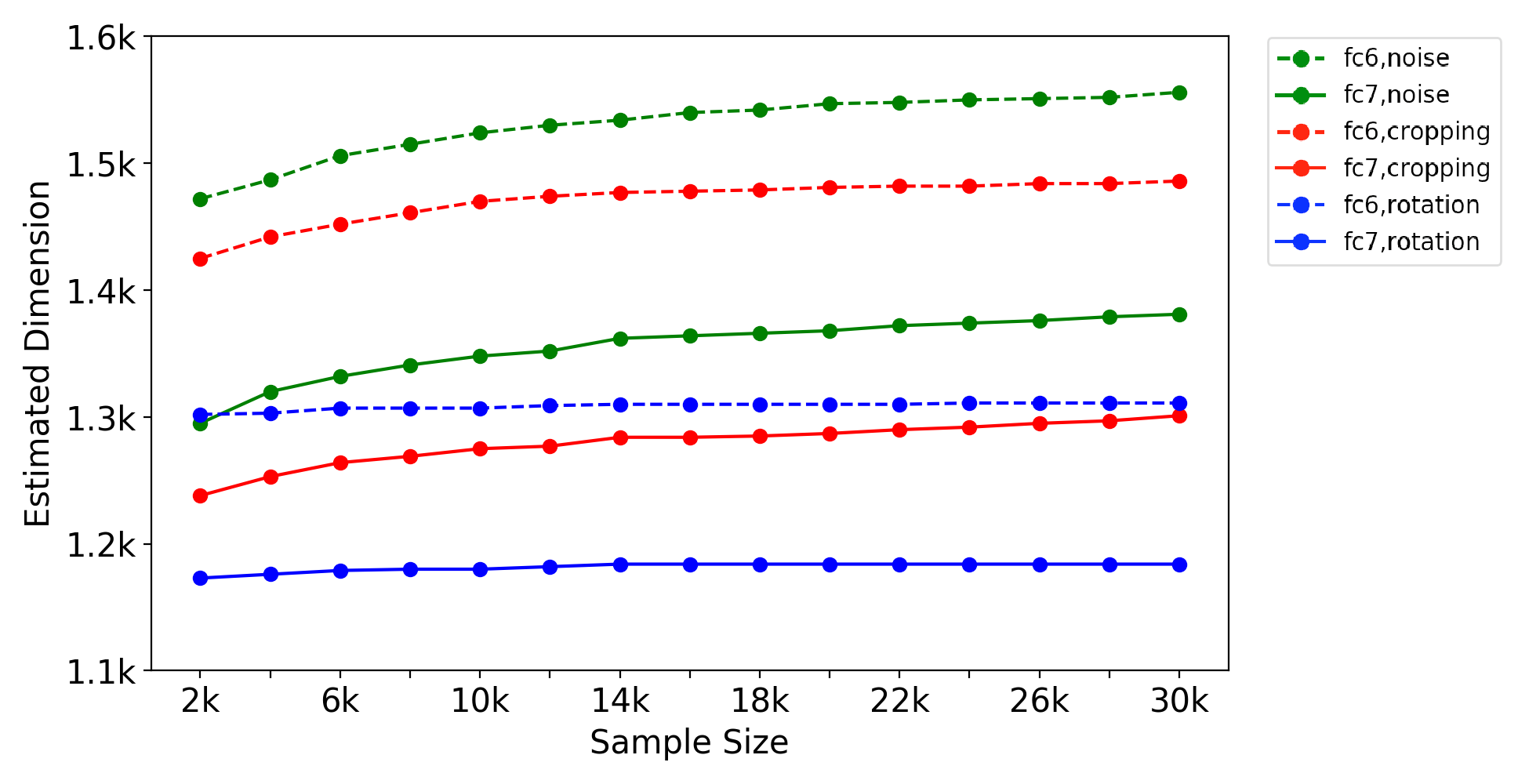
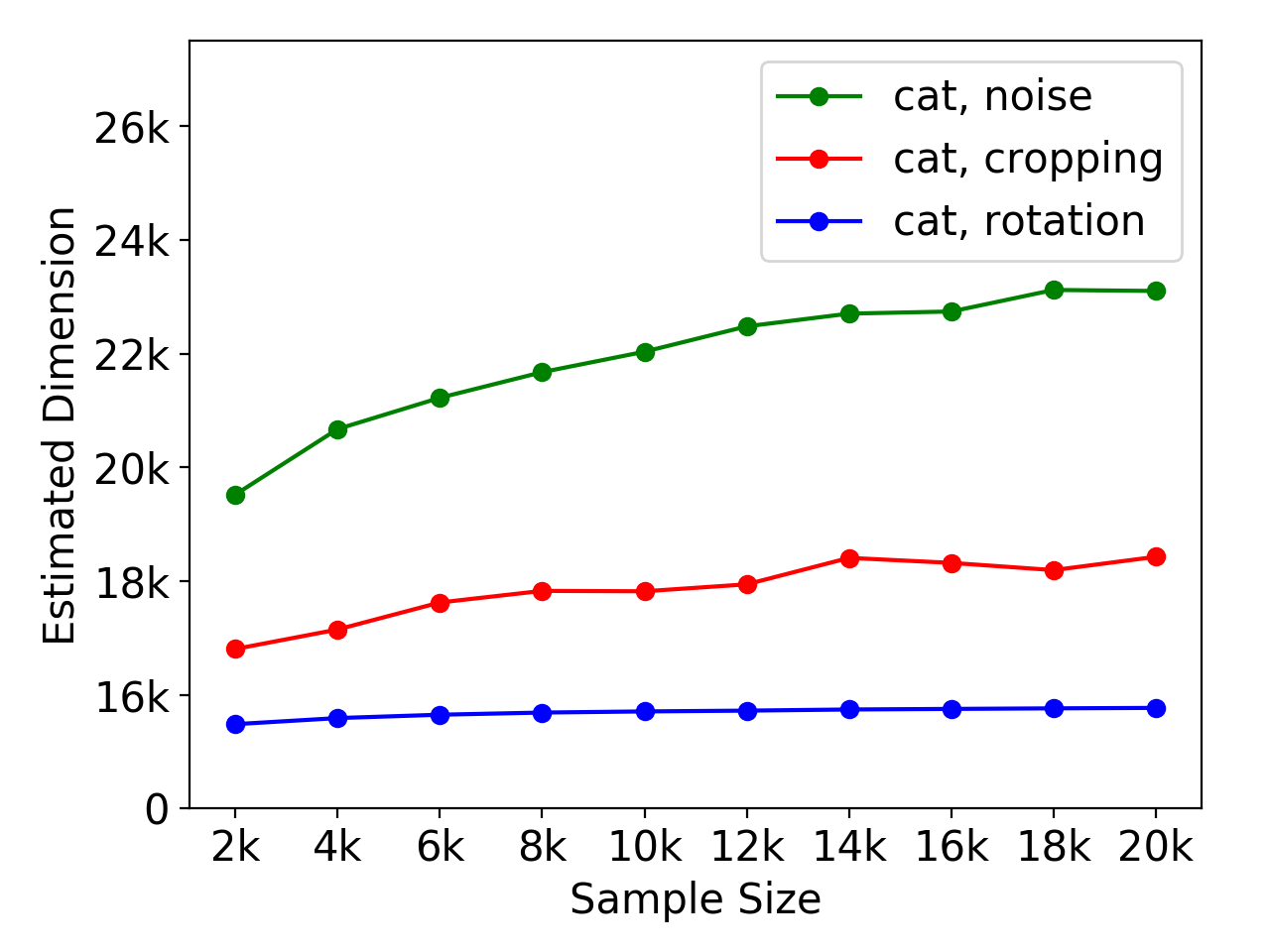
Influence on the estimated dimension by the data size. Figure 8 shows the estimated dimension versus the augmentation data size. The dimension grows slowly with the growth of the data size. Although the augmentation data scale influences the estimated dimension, the growth on the dimension along with the data size is fairly small. The dimension only grows by less than 3% as the data size triples. Thus, it is reasonable to use a fairly small data set to estimate the dimension. More importantly, as shown in Figure 8, such rule can also be generalized to calculate the estimated dimension of the convolutional layers.
Rule 2. We can determine the local tangent hyperplane’s estimated dimension of the manifold in a layer (fully connected or convolution) using a fairly small data cluster size, for example, 8k.
size in Conv5_4 layer.

dimension for maxpooling5.
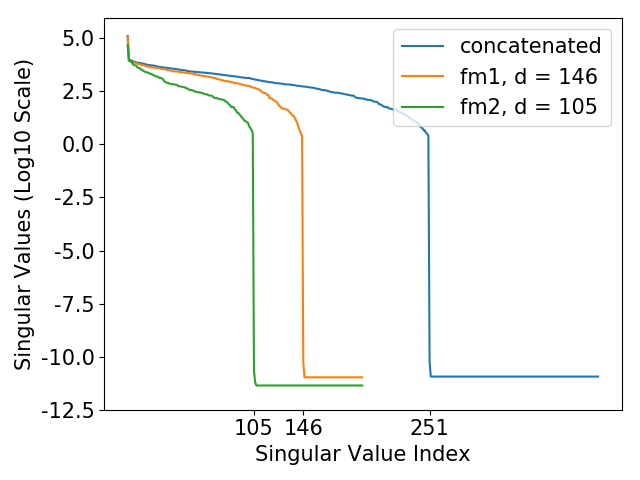
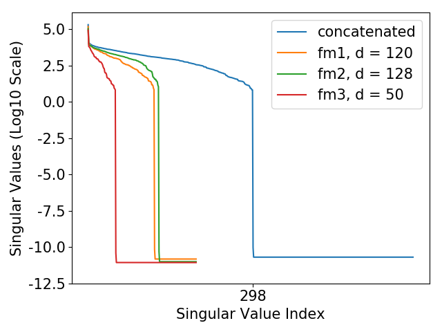
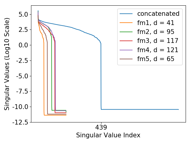
Estimated dimension and concatenated/original dimension. We randomly pick feature maps in layer Conv5_1 and calculate the estimated dimension as well as concatenated dimension. The result of are as shown in Figure 5. For the result of , see Table 3 in Appendix. The estimated dimension is very close to the corresponding concatenated dimension. Thus, we can use the estimated dimension to approximate the concatenated dimension.
We then pick all feature maps in maxpooling5, and calculate the estimated dimension, original dimension. Figure 8 shows that start from 8k of the data size, the estimated dimension is close to the original dimension. Thus, we can use a small amount of 8000 images to approximate the original dimension using the estimated dimension.
When the data cluster size is insufficient, assuming the local tangent hyperplane of the manifold is -dimensional, the result will be strictly restricted by the number of input images when . So that the concatenated dimension or original dimension we calculate would be almost equal to for small , while estimated dimension is a summation which can approximate .
Rule 3. The original dimension of the local tangent hyperplane can be approximated by the estimated dimension using a fairly small size of dataset, for example 8000.
6 Dimensions of the Deep Manifolds
For each of the three categories, Persian Cat (n02123394), Container Ship (n03095699) and Volcano (n09472597) in ImageNet, we randomly choose three images of high probability and determine the estimated dimensions based on the three rules drawn in Section 5.
Dimensions for Conv5 and fully connected layers. For Conv5 and fully connected layers, we summarize the average of the estimated dimensions in Table 1 and Figure 10. The estimated dimension gradually declines from Conv5_1 to fc8. For fc6 and fc7, the activations lie in a low-dimension manifold embedded in the 4096-dimension space. For fc8, the manifold’s dimension is exactly 1000. It makes sense as fc8 is directly linked to the final classification prediction, it is in full rank to achieve a higher performance. The dimensions of the three categories are close to each other and decline quickly inside the four convolutional layers and the last maxpooling layer.
| 5_1 | 5_2 | 5_3 | 5_4 | pool5 | fc6 | fc7 | fc8 | |
|---|---|---|---|---|---|---|---|---|
| cat | 59946 | 51347 | 47958 | 29834 | 8358 | 1580 | 1506 | 1000 |
| ship | 58329 | 44968 | 39781 | 25267 | 8851 | 1577 | 1691 | 1000 |
| volcano | 62540 | 53136 | 51939 | 30862 | 10816 | 2163 | 1887 | 1000 |
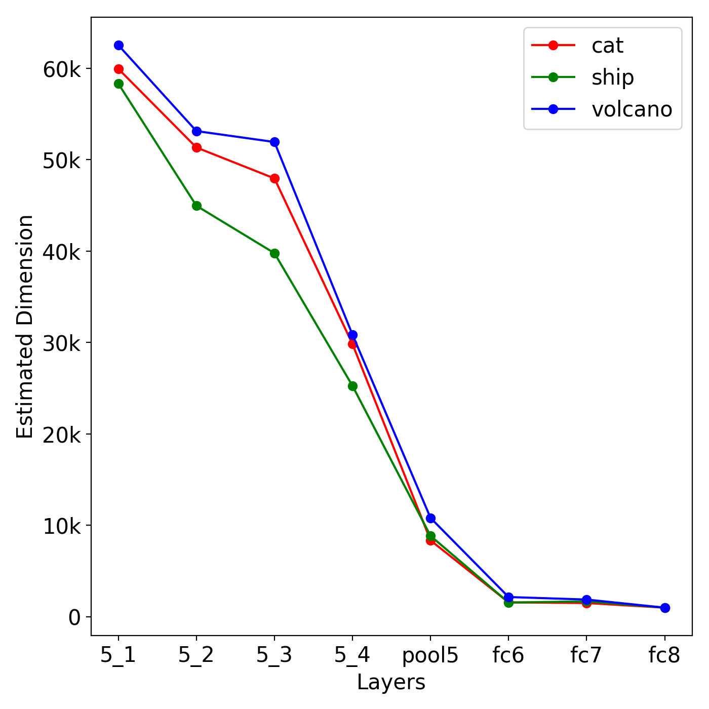
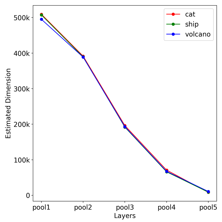
Dimensions for maxpooling layers. We illustrate the average of the estimated dimensions in Figure 10 all maxpooling layers. The dimensions of the three categories coincide with each other and decline quickly for deep pooling layers.
7 Conclusions
Through extensive experiments, we found that there exists a dramatic drop for the singular values of the fully connected layers or a single feature map of the convolutional layer, and the dimension of the concatenated feature vector almost equals the summation of the dimension of each feature map for several feature maps randomly picked. Based on the interesting observations we obtained, we developed an efficient and effective SVD based method to estimate the local dimension of deep manifolds in the VGG19 neural network. We found that the dimensions are close for different images of the same category and even images of different categories, and the dimension declines quickly along the convolutional layers and fully connected layers. Our results support the low-dimensional manifold hypothesis for deep networks, and our exploration helps unveiling the inner organization of deep networks. Our work will also inspire further possibility of observing every feature map separately for the dimension of convolutional layers, rather than directly working on the whole activation feature maps, which is costly or even impossible for the current normal computing power.
Acknowledgments
The work is supported by National Natural Science Foundation of China (61772219, 61472147) and US Army Research Office (W911NF-14-1-0477).
References
- Bengio & Monperrus (2005) Yoshua Bengio and Martin Monperrus. Non-local manifold tangent learning. In Advances in Neural Information Processing Systems, pp. 129–136, 2005.
- Cayton (2005) Lawrence Cayton. Algorithms for manifold learning. Univ. of California at San Diego Tech. Rep, 12:1–17, 2005.
- Dosovitskiy & Brox (2016) Alexey Dosovitskiy and Thomas Brox. Inverting visual representations with convolutional networks. pp. 4829–4837, 2016.
- Goodfellow et al. (2016) Ian Goodfellow, Yoshua Bengio, and Aaron Courville. Deep Learning. MIT Press, 2016.
- Haro et al. (2008) Gloria Haro, Gregory Randall, and Guillermo Sapiro. Translated poisson mixture model for stratification learning. Int. J. Comput. Vision, 80(3):358–374, 2008.
- He et al. (2016) Kun He, Yan Wang, and John Hopcroft. A powerful generative model using random weights for the deep image representation. In NIPS, pp. 631–639, 2016.
- Johnstone (2001) Iain M. Johnstone. On the distribution of the largest eigenvalue in principal components analysis. Ann. Statist., 29(2):295–327, 2001.
- Kingma et al. (2014) Diederik P Kingma, Shakir Mohamed, Danilo Jimenez Rezende, and Max Welling. Semi-supervised learning with deep generative models. In NIPS, pp. 3581–3589, 2014.
- Levina & Bickel (2005) Elizaveta Levina and Peter J. Bickel. Maximum likelihood estimation of intrinsic dimension. In L. K. Saul, Y. Weiss, and L. Bottou (eds.), NIPS, pp. 777–784. MIT Press, 2005.
- Li & Yuan (2017) Yuanzhi Li and Yang Yuan. Convergence analysis of two-layer neural networks with relu activation. CoRR, abs/1705.09886, 2017.
- Little et al. (2009) A. V. Little, J. Lee, Y. M. Jung, and M. Maggioni. Estimation of intrinsic dimensionality of samples from noisy low-dimensional manifolds in high dimensions with multiscale svd. In 2009 IEEE/SP 15th Workshop on Statistical Signal Processing, pp. 85–88, 2009.
- Mahendran & Vedaldi (2015) Aravindh Mahendran and Andrea Vedaldi. Understanding deep image representations by inverting them. In CVPR, pp. 5188–5196, 2015.
- Narayanan & Mitter (2010) Hariharan Narayanan and Sanjoy Mitter. Sample complexity of testing the manifold hypothesis. In NIPS, pp. 1786–1794, 2010.
- Rahimi & Recht (2009) Ali Rahimi and Benjamin Recht. Weighted sums of random kitchen sinks: Replacing minimization with randomization in learning. In NIPS, pp. 1313–1320, 2009.
- Rifai et al. (2011) Salah Rifai, Yann N Dauphin, Pascal Vincent, Yoshua Bengio, and Xavier Muller. The manifold tangent classifier. In NIPS, pp. 2294–2302, 2011.
- Saxe et al. (2011) Andrew Saxe, Pang W Koh, Zhenghao Chen, Maneesh Bhand, Bipin Suresh, and Andrew Y Ng. On random weights and unsupervised feature learning. In ICML, pp. 1089–1096, 2011.
- Simonyan & Zisserman (2014) K. Simonyan and A. Zisserman. Very Deep Convolutional Networks for Large-Scale Image Recognition. ArXiv e-prints, 2014.
- Strang et al. (1993) Gilbert Strang, Gilbert Strang, Gilbert Strang, and Gilbert Strang. Introduction to linear algebra, volume 3. Wellesley-Cambridge Press, MA, 1993.
- Van der Maaten & Hinton (2008) Laurens Van der Maaten and Geoffrey Hinton. Visualizing data using t-sne. Journal of Machine Learning Research, 9, 2008.
- Weinberger et al. (2004) Kilian Q Weinberger, Fei Sha, and Lawrence K Saul. Learning a kernel matrix for nonlinear dimensionality reduction. In ICML, pp. 106, 2004.
- Zhang et al. (2017) Chiyuan Zhang, Samy Bengio, Moritz Hardt, Benjamin Recht, and Oriol Vinyals. Understanding deep learning requires rethinking generalization. In ICLR, 2017.
Appendix

| Layer |
|
|
|
||||||
|---|---|---|---|---|---|---|---|---|---|
| conv1 | 224224 | 64 | 3211264 | ||||||
| maxpooling1 | 112112 | 64 | 802816 | ||||||
| conv2 | 112112 | 128 | 1605632 | ||||||
| maxpooling2 | 5656 | 128 | 401408 | ||||||
| conv3 | 5656 | 256 | 802816 | ||||||
| maxpooling3 | 2828 | 256 | 200704 | ||||||
| conv4 | 2828 | 512 | 401408 | ||||||
| maxpooling4 | 1414 | 512 | 100352 | ||||||
| conv5 | 1414 | 512 | 100352 | ||||||
| maxpooling5 | 77 | 512 | 25088 | ||||||
| fc6 | 4096 | 1 | 4096 | ||||||
| fc7 | 4096 | 1 | 4096 | ||||||
| fc8 | 1000 | 1 | 1000 |
| Sample1 | Sample2 | Sample3 | |
|---|---|---|---|
| Dim.0 | 124 | 131 | 158 |
| Dim.1 | 112 | 163 | 80 |
| Dim.2 | 141 | 126 | 62 |
| Dim.3 | 128 | 95 | 120 |
| Dim.4 | 141 | 156 | 61 |
| Dim.5 | 78 | 129 | 155 |
| Dim.6 | 96 | 152 | 112 |
| Dim.7 | 113 | 103 | 116 |
| Dim.8 | 123 | 62 | 118 |
| Dim.9 | 157 | 120 | 128 |
| Dim.estim | 1213 | 1237 | 1110 |
| Dim.concat | 1213 | 1237 | 1110 |