Abstract

Robust analysis of coauthorship networks is based on high quality data. However, ground-truth data are usually unavailable. Empirical data suffer several types of errors, a typical one of which is called merging error, identifying different persons as one entity. Specific features of authors have been used to reduce these errors. We proposed a Bayesian model to calculate the information of any given features of authors. Based on the features, the model can be utilized to calculate the rate of merging errors for entities. Therefore, the model helps to find informative features for detecting heavily compromised entities . It has potential contributions to improving the quality of empirical data.

Introduction

Studies of coauthorship networks with large scale provide a bird-eye view of collaboration patterns in scientific society, and have become an important topic of social sciences[2, 1, 3]. Ambiguities exist in the collection of coauthorship data, which manifest themselves in two ways: one person is identified as two or more entities (splitting error); two or more persons are identified as one entity (merging error). Here persons refer to authors, and entities refer to nodes of coauthorship networks[4]. These errors make the collected data deviate from ground truth. Merging errors deflate the number of persons, the average shortest path, and the global clustering coefficient[7, 5, 6]. These errors also inflate the average number of the papers per author, the average number of the collaborators per author, and the size of giant component.

Analysis drawn on imperfect data is at risk. However, in data-intensive research, ground-truth data are often unavailable. In social network analysis, there exist extensive research on detecting and reducing data errors[8], especially on missing and spurious connections[9, 10, 11]. In the case of coauthorship networks, such research is called name disambiguation. For the authors of different papers with the same name, it is reasonable to assume that the more similar (such coauthors, email, etc.) these authors’ features are, the more likely they are of the same person. Therefore, a range of name disambiguation methods have been provided to reduce the merging and splitting errors, based on the features extracted from the contents of publications (such as email address, title, abstract, and references), from the web information of authors, and so on[12, 14, 13]. Those methods have been proved to be effective in specific cases[15, 16, 17, 18, 19]. Utilizing the features of authors efficiently is still a challenge and needs further research[20]. Here we do not consider the specific techniques of reducing errors, but want to know the merging error level of empirical data. Whether the level is severe enough to warrant data reliability? Which data are most heavily compromised?

In the view of Bayesians, inference from data is the revision of a given opinion in the light of relevant new information[21]. Therefore, we proposed a Bayesian model for utilizing observed author features to revise the opinion reflected by empirical data. Our model is based on the Bayesian model provided by Newman, which is designed to infer network structures[22]. The novel aspect here is that we utilized the prior knowledge of error rates. This is inspired by the Bayesian model provided by Butts, which is designed to infer the errors of networks[23]. The different aspect from Butts’ model is that we removed the hyperparameters of the distribution of ground-truth data. Our model can be utilized to calculate the information of authors’ features. When knowing which features are informative, we can use them to calculate the rate of merging errors over entities effectively, and then find those entities heavily compromised. Therefore, the model has the ability to assess the error level of coauthorship networks, and to estimate the number of nodes for those networks. We demonstrated model functions by using the names of coauthors, a feature used in many name disambiguation methods.

This report is organized as follows: the model is described in Section 2; its demonstration is shown Section 3; the discussion and conclusions are drawn in Section 4.

The model

Consider $N_{l}$ authors to be of an entity $l$. Denote the ground-truth relationship by $A_{ij}$ for all author pair $(i,j)$, where $A_{ij}=1$ means the pair are actually one person, and $A_{ij}=0$ means not. That is, the probability of authors $i$ and $j$ being the same person depends only on $A_{ij}$. This dependence can be parameterized by two quantities: the false negative rate $e^{-}$, and the false positive rate $e^{+}$ that is merging error rate. Note that $e^{-}$ is not splitting error rate, because it does not address the case that a person is regarded as several entities.

Assume that the prior distribution of $A_{ij}$ is determined via a parameter $\rho\in[0,1]$, the specific form of which adopted here is $A_{ij}\sim\rho^{A_{ij}}(1-\rho)^{1-A_{ij}}$. Then the likelihood function of $\rho$ is

$$L(\rho) =\prod_{i<j}\rho^{A_{ij}}(1-\rho)^{1-A_{ij}}.$$ (1)

Maximizing it respect to $\rho$ gives rise to

$$\rho =\frac{2\sum_{i<j}A_{ij}}{N_{l}(N_{l}-1)}.$$ (2)

Assume that the error rates $e^{+}$ and $e^{-}$ are drawn independently from two Beta distributions, namely $e^{+}\sim\mathrm{Beta}(\alpha^{+},\beta^{+})$ and $e^{-}\sim\mathrm{Beta}(\alpha^{-},\beta^{-})$. The choice of the parameters of these distributions reflects the prior knowledge regarding the errors of data. The density function of a Beta distribution $\mathrm{Beta}(\alpha,\beta)$ is $\mathrm{Beta}(x|\alpha,\beta)=\Gamma(\alpha+\beta)x^{\alpha-1}(1-x)^{\beta-1}/(\Gamma(\alpha)\Gamma(\beta))$, where $x\in[0,1]$.

Specify a real value $N_{ij}$ to quantify any observed features (such as coauthor names, affiliation, email, and so on) of author pair $(i,j)$, and a real value $E_{ij}$ to quantify the similarity between their features. So $E_{ij}/N_{ij}\in[0,1]$ expresses the similar level between $i$ and $j$. Assume that the probability of observing the features and similarity (quantified as $E_{ij}$ and $N_{ij}$) conditional on $A_{ij}$, $e^{+}$ and $e^{-}$ is the following Bernoulli mixture

$$p(E_{ij},N_{ij}|A_{ij},e^{+},e^{-})=B(E_{ij},N_{ij}|1-e^{-})^{A_{ij}}\times B(E_{ij},N_{ij}|e^{+})^{(1-A_{ij})},$$ (3)

where $B(E_{ij},N_{ij}|x)$ is the density $\mathrm{Beta}(x|E_{ij}+1,N_{ij}-E_{ij}+1)$ for $x\in\{e^{+},1-e^{-}\}$.

Our model is designed to calculate the posteriors of $A_{ij}$ and $e^{\pm}$ given $E_{ij}$ and $N_{ij}$. Note that its aim is not to correcting data errors, but to assessing the merging error level of empirical data. Fig. 1 shows an illustration of the model.

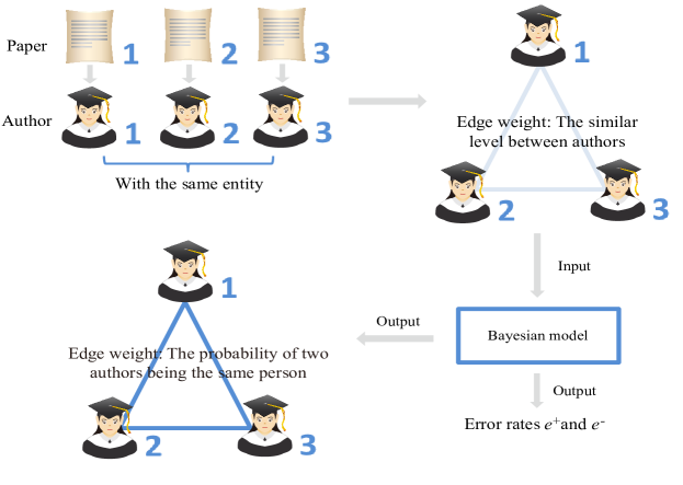
Figure 1: Illustration of the Bayesian model. The similar level between authors is calculated based on author features, such as full name, coauthors, affiliation, email address, etc.

The unnormalized posterior of $A_{ij}$ given $N_{ij}$, $E_{ij}$, $e^{+}$ and $e^{-}$ is

$$p(A_{ij}|E_{ij},N_{ij},e^{+},e^{-}) \propto p(E_{ij},N_{ij}|A_{ij},e^{+},e^{-})p(A_{ij})$$ (4)

$$= B(E_{ij},N_{ij}|1-e^{-})^{A_{ij}}\times B(E_{ij},N_{ij}|e^{+})^{(1-A_{ij})}$$

$$\times\rho^{A_{ij}}(1-\rho)^{1-A_{ij}}$$

Eq. (4) is an unnormalized form of a Beta density. Maximizing it with respect to $A_{ij}$ gives rise to

$${A}_{ij}=\frac{\rho(1-e^{-})^{E_{ij}}{e^{-}}^{N_{ij}-E_{ij}}}{\rho(1-e^{-})^{E_{ij}}{e^{-}}^{N_{ij}-E_{ij}}+(1-\rho){e^{+}}^{E_{ij}}(1-e^{+})^{N_{ij}-E_{ij}}}.$$ (5)

The same logic can be utilized for $e^{+}$, namely

$$p(e^{+}|(E_{ij}),(N_{ij}),(A_{ij}),e^{-}) \propto p((E_{ij}),(N_{ij})|(A_{ij}),e^{+},e^{-})p(e^{+})$$

$$= p(e^{+})\prod_{i<j}p(E_{ij},N_{ij}|A_{ij},e^{+},e^{-})$$

$$\propto \mathrm{Beta}(e^{+}|\alpha^{+}+1,\beta^{+}+1)\times\prod_{i<j}B(E_{ij},N_{ij}|e^{+})^{1-A_{ij}}$$

$$\propto {e^{+}}^{\sum_{i<j}E_{ij}(1-A_{ij})+\alpha^{+}}\times(1-e^{+})^{\sum_{i<j}(N_{ij}-E_{ij})(1-A_{ij})+\beta^{+}},$$ (6)

where $(A_{ij})$, $(E_{ij})$ and $(N_{ij})$ are $N_{l}\times N_{l}$ matrixes. Maximize it with respect to $e^{+}$ and perform the same calculation for $e^{-}$. Then, we obtained

$${{e}}^{+} =\frac{\sum_{i<j}E_{ij}(1-A_{ij})+\alpha^{+}}{\sum_{i<j}N_{ij}(1-A_{ij})+\alpha^{+}+\beta^{+}},$$

$${{e}}^{-} =1-\frac{\sum_{i<j}E_{ij}A_{ij}+\beta^{-}}{\sum_{i<j}N_{ij}A_{ij}+\alpha^{-}+\beta^{-}}.$$ (7)

Value $\alpha^{\pm}$ and $\beta^{\pm}$. Initialize $e^{\pm}$ and $\rho$. Iterate Eqs. (3), (5) and (The model) until convergence or the maximum number of iterations is reaching. Then we can obtain $({A}_{ij})$, ${e}^{\pm}$ and $\rho$. Table 1 shows this process.

Table 1: The process of the presented model.

Input: Observed $N_{l}\times N_{l}$ matrixes $(E_{ij})$ and $(N_{ij})$ for entity $l$.

Value $\alpha^{+}$, $\alpha^{-}$, $\beta^{+}$ and $\beta^{-}$;

Initialize $e^{+}$, $e^{-}$ and $\rho$;

Repeat:

calculate $A_{ij}$ through Eq. (5);

renew $e^{+}$ and $e^{-}$ through Eqs. (The model);

renew $\rho$ through Eq. (3).

Until convergence or the maximum number of iterations is reached.

Output: $(A_{ij})$, $e^{\pm}$ and $\rho$.

The values of error rates help us evaluate the contribution of the given features. Error rates $e^{+}\rightarrow\alpha^{+}/(\alpha^{+}+\beta^{+})$ and $e^{-}\rightarrow\alpha^{-}/(\alpha^{-}+\beta^{-})$ imply that the features, reflected by $E_{ij}$ and $N_{ij}$, carries no information. More broadly, the carried information can be measured by

$$I=1-(e^{+}+e^{-}).$$ (8)

For example, if a feature with $E_{ij}=N_{ij}$ for any $i$ and $j$, then $A_{ij}=1$ is a solution of Eq. (5). Submitting the solution to Eqs. (The model) gives rise to ${e}^{+}=\alpha^{+}/(\alpha^{+}+\beta^{+})$, ${e}^{-}=\alpha^{-}/({N_{l}(N_{l}-1)/2+\alpha^{-}+\beta^{-}})$, which are free of the feature. It means no information is carried by the feature. If a feature with $E_{ij}=0$ for any $i$ and $j$, then $A_{ij}=0$ is a solution of Eq. (5), then the error rates ${e}^{+}=\alpha^{+}/(N_{l}(N_{l}-1)/2+\alpha^{+}+\beta^{+})$, ${e}^{-}=\alpha^{-}/({\alpha^{-}+\beta^{-}})$, which are also free of the feature.

The formula (8) assesses the contribution of the given features to the improvement of the quality of empirical data. The contribution here means that using the feature helps us decrease the uncertainty of estimating the ground-truth data, namely $(A_{ij})$ for any $i$ and $j$. Increasingly positive or negative value of $I$ indicates increasing or decreasing information of the feature[23]. Based on the features with positive information, Eqs. (The model) can tell us whether the error level is severe enough to warrant data reliability, and which name entities are most heavily compromised.

Eq. (2) tells us the probability of $N_{l}$ authors being the same person. With the probability $\rho$, the estimated number of the persons wrongly merged is $(1-\rho)({N}_{l}-1)$. Adding $1$ to this number gives rise to the evaluated number of the persons with entity $l$

$$\hat{N}_{l} =(1-\rho)N_{l}+\rho.$$ (9)

Therefore, we obtained the evaluated number of a dataset’s persons, namely $\hat{N}=\sum_{l}\hat{N}_{l}$.

Demonstration of model functions

The feature of coauthors (e. g. the names of coauthors) has been adopted by a range of name disambiguation methods[20]. Here we used coauthors’ name to demonstrate model functions on three sets of papers: SCAD-zbMATH (28,321 mathematical papers during 1867–1999), PNAS-2007–2015 (36,732 papers of Proceedings of the National Academy of Sciences), and PRE-2007–2016 (24,079 papers of Physical Review E). The first set only contains the papers for which all authors are manually disambiguated[24]. The ground-truth entities of authors are denoted as author id. The other two sets are collected from Web of Science (www.webofscience.com), where their papers are published during those years in their name. They contain the names of authors on papers.

We applied our model to the entities generated through author id (zbMATH-a), to the entities generated through surname and the initials of all provided given names (PNAS-a, PRE-a), to the entities generated through the names on papers (zbMATH-b, PNAS-b, PRE-b), and to the entities through short name, namely surname and the initial of the first given name (zbMATH-c, PNAS-c, PRE-c). Table 2 shows certain statistical indexes for the nine datasets.

Table 2: Specific statistical indexes of empirical data.

Data	$N$	$M$	$a$	$b$	$c$	$d$
zbMATH-a	2,946	28,321	4.177	11.48	1.194	0.593
zbMATH-b	4,696		2.621	7.200		0.586
zbMATH-c	2,919		4.216	11.58		0.661
PNAS-a	136,322	34,630	17.82	1.793	7.059	0.310
PNAS-b	161,780		15.02	1.511		0.259
PNAS-c	115,463		21.04	2.117		0.356
PRE-a	30,552	21,634	7.495	2.365	3.339	0.412
PRE-b	36,915		6.203	1.957		0.355
PRE-c	27,925		8.201	2.587		0.443

Index $N$: the number of entities, $M$: the number of hyperedges, $a$: the average degree, $b$: the average hyperdegree, $c$: the average size of hyperedges, $d$: the proportion of the entities with hyperdegree$>1$.

Given a similar level $E_{ij}/N_{ij}$ between any two merged authors $i$ and $j$, we can demonstrate model functions on empirical data. Let $E_{ij}=1$ if $i$ and $j$ have some coauthors sharing the same short name, $E_{ij}=0$ if not, and $N_{ij}=1$. Note that the matrix $(E_{ij})$ also suffers merging errors, so it would not be always helpful for name disambiguation. Even without merging errors, its contributions would also be limited, because some authors would publish papers with different authors.

We run the model with the two settings in Table 3 for parameters ($\alpha^{\pm}$, $\beta^{\pm}$) and initializations ($e^{\pm}$, $\rho$). Our model with Setting 2 is just the model of Newman[22]. The reason of using Setting 1 is that it satisfies following restrictions. The number of pairs $\epsilon=N_{l}(N_{l}-1)/2$, which gives rise to $\alpha^{+}+\beta^{+}=\alpha^{-}+\beta^{-}=\epsilon$. When $E_{ij}=1$ for all possible $i$ and $j$, we let $e^{+}=1$, $e^{-}=0$ and $\rho=1$, because all of the $N_{l}$ authors are regarded as the same person. It gives rise to $\alpha^{-}=\beta^{+}=0$. When $E_{ij}=0$, we let $e^{+}=0$, $e^{-}=1$ and $\rho=0$, because all of the $N_{l}$ authors are regarded as different persons. It gives rise to $\alpha^{+}=\beta^{-}=0$.

We compared the results of our model with those of Newman’s model. The outputs of the two models are listed in Table 4. For zbMATH-a,b,c, their estimated number of authors $\hat{N}$ deviates far away from the number of entities $N$. There are 59.3% authors published more than one paper. The average hyperdegree of authors is $11.48$. Therefore, the size of matrix $(E_{ij})$ for over 59.3% entities is larger than $11\times 11$. Meanwhile, the average number of the authors per paper is only $1.194$, thus $(E_{ij})$ is sparse for many entities. It gives rise to the low value of $\rho$ for those entities, and thus leads to the large value of the ratio $\hat{N}/N$.

Table 3: The settings of parameters and initializations.

Setting 1: $\alpha^{+}=\beta^{-}=\epsilon\rho_{0}$, $\alpha^{-}=\beta^{+}=\epsilon(1-\rho_{0})$, $e^{+}=\rho=\rho_{0}$ and $e^{-}=1-\rho_{0}$,

where $\rho_{0}=\sum_{l,k}E_{lk}/\sum_{l,k}N_{lk}$, and $\epsilon={N_{l}(N_{l}-1)}/{2}$.

Setting 2: $\alpha^{+}=\beta^{-}=\alpha^{-}=\beta^{+}=0$, $e^{+}$, $e^{-}$ and $\rho$ are random variables drawn

from the uniform distribution $U(0,1)$.

Table 4: The comparisons between the outputs of our model and those of Newman’s model.

Data	$\hat{N}$	$\hat{N}/N$	$\bar{{e}}^{+}$	$\bar{{e}}^{-}$	$\bar{{I}}$	$\bar{\rho}$
zbMATH-a	30,943	1050.4%	0.304	0.696	0.000	0.304
	19,072	647.4%	0.313	0.692	-0.004	0.499
zbMATH-b	30,722	654.2%	0.247	0.753	0.000	0.247
	19,036	405.3%	0.255	0.747	-0.001	0.502
zbMATH-c	21,218	726.9%	0.281	0.719	0.000	0.281
	18,372	629.4%	0.288	0.711	0.001	0.504
PNAS-a	201,699	148.0%	0.537	0.463	0.000	0.537
	190,445	139.7%	0.546	0.455	-0.001	0.500
PNAS-b	198,231	122.5%	0.637	0.363	0.000	0.637
	203,420	125.7%	0.643	0.357	0.001	0.500
PNAS-c	186,601	161.6%	0.469	0.531	0.000	0.469
	180,628	156.4%	0.479	0.519	0.002	0.498
PRE-a	53,230	174.2%	0.585	0.415	0.000	0.585
	51,387	168.2%	0.594	0.406	0.000	0.501
PRE-b	53,159	144.0%	0.646	0.354	0.000	0.646
	54,450	147.5%	0.653	0.347	0.001	0.500
PRE-c	50,503	180.9%	0.554	0.446	0.000	0.554
	49,654	177.8%	0.564	0.438	-0.002	0.498

For each sub-table, the outputs of our model are listed in the first row, and those of Newman’s model in the second row. Index $\hat{N}$: the evaluated number of entities, $\hat{N}/N$: the ratio of $\hat{N}$ to the number of entities $N$, $\bar{\rho}$: the average of entities’ $\rho$ defined by Eq. (2), $\bar{e}^{\pm}$: the average of entities’ ${e}^{\pm}$ defined by Eqs. (The model), and $\bar{{I}}$: the average of entities’ $I$ defined by the formula (8).

The ratios of PNAS-a,b,c are smaller than those of zbMATH-a,b,c, and those of PRE-a,b,c, respectively. For PNAS-a,b,c, their average hyperdegree is relatively small, and their average degree is relatively large. Therefore, their $(E_{ij})$ is dense and has a small size on average, compared to that of other datasets. It gives rise to a small value of their ratio $\hat{N}/N$.

Fig. 2 shows the distributions of false positive rates and those of false negative rates for the datasets with the suffix -a. We found that the trends of those distributions calculated through our model and those through Newman’s model are the same. The number of entities with error rate $1$ or $0$ is large, compared with that of any other value. The distributions of false positive rates are symmetric to the corresponding distributions of false negative rates about $0.5$. This is because that coauthors’ short name carries null information, namely $e^{+}+e^{-}\approx 1$.

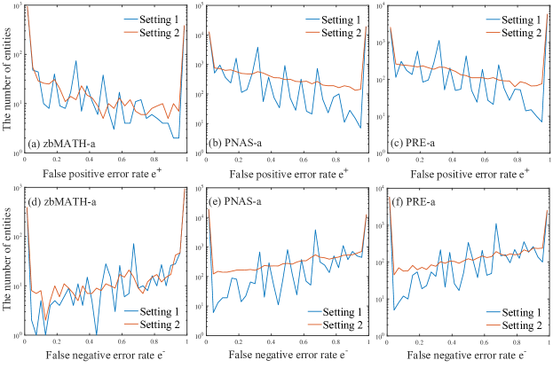
Figure 2: The distributions of error rates. Panels show the comparisons between the distributions calculated through our model (Setting 1) and those through Newman’s model (Setting 2).

Fig. 3 shows these distributions for the datasets with suffixes -b and -c. We found that these distributions for the entities obtained by different methods are positively correlated. In fact, the Pearson correlation coefficient of each pair from the datasets with the same prefix is larger than $0.95$. However, the error rates are different for the entities obtained through different methods. The highly positive correlations imply that the feature of coauthors’ short name is insensitive to merging errors.

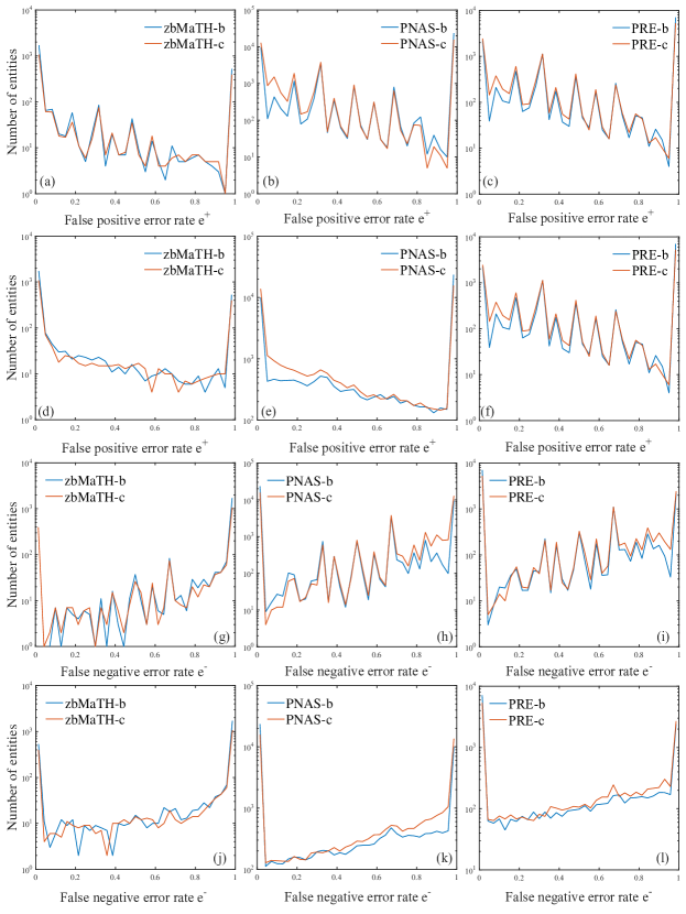
Figure 3: The error distributions of the entities generated through different methods. The entities of the datasets with suffix -b are generated through the names on papers, and those with suffix -c are generated through short name. The distributions in Panels (a-c, g-i) are calculated through our model, and those in Panels (d-f, j-l) are calculated through Newman’s model.

Because of the positive correlations, we now only discuss the model outputs for the datasets with suffix -a. Fig 4 shows the relationship between the model outputs ($I$, $\hat{N}$, and ${e}^{\pm}$) and hyperdegree. We found that the average value of the false positive rates over $k-$hyperdegree entities decreases with the growth of $k$. The case for the false negative error rates and that for the estimated numbers of persons are reverse. Underlying these phenomena is that the average value of $A_{ij}$ over $k-$hyperdegree entities decreases with the growth of $k$. This is caused by the property of empirical data: the probability that the authors of an entity have a coauthor with the same short name decreases with the growth of the entity’s hyperdegree, on average.

These phenomena shown in Fig 4 mean disambiguating by using the short names (surname and the initial of the first given name) of coauthors surfers high risk of false positive errors but low risk of false negative errors for the entities with a small hyperdegree. The case is reverse for the entities with a large hyperdegree. However, Fig 4 also shows that the average value of the information $I$ over $k-$hyperdegree entities is around $0$ for any possible $k$. It means that synthetically considering both risks, the short names of coauthors carry null information for improving the quality of the empirical datasets.

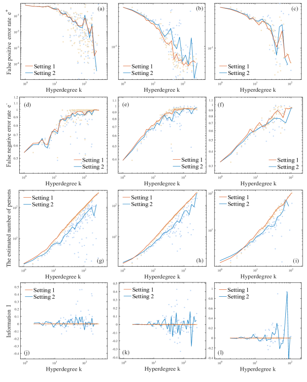
Figure 4: The relationship between hyperdegree and model outputs. The inputs of models are the datasets with suffix-a. Panels show the average value of each output (i. e., $e^{+}$, $e^{-}$, $\hat{N}_{l}$ and $I$) over the entities with hyperdegree $k$ (red circles, blue squares). These average values are binned on abscissa axes to extract the trends hiding in noise (red and blue lines).

Discussion and conclusions

A Bayesian model is provided to measure the quality of coauthorship data based on author features, and to assess the contribution of author features to the improvement of data quality. With the model, we can calculate the distribution of merging errors over the entities of authors, inferring the number of persons. Even where our model does not provide substantial uncertainty reduction (e. g., where only the information of coauthors’ name is available), it may still be of use in its ability to provide a theoretical assessment of merging error level for coauthorship data.

Network scale and data accuracy are two irreconcilable challenges for coauthorship analysis. It is easy to correct a small dataset, but the results obtained by studying small datasets are incomplete. Meanwhile, correcting a large dataset is a time-consuming mission. Even corrected data with large scale are available, they still cannot cover all coauthorship. Many existing results of coauthorship are based on incomplete or imperfect coauthorship data[25, 27, 26]. Our model has the potential to be extended for assessing the confidence level of these results, thus would have clear applicability to empirical research.

Funding

ZX acknowledges support from National Science Foundation of China (NSFC) Grant No. 61773020.

References

- 1. Glänzel W, Schubert A (2004) Analysing scientific networks through co-authorship. Handbook of quantitative science and technology research, 257-276.
- 2. Adams J (2012) Collaborations: The rise of research networks. Nature 490: 335-336.
- 3. Uzzi B, Mukherjee S, Stringer M, Jones B (2013) Atypical combinations and scientific impact. Science 342(6157): 468-472.
- 4. Smalheiser NR, Torvik VI (2009) Author name disambiguation. Annu Rev Inform Sci Technol 43: 287-313.
- 5. Milojević S (2013) Accuracy of simple, initials-based methods for author name disambiguation. J Informetr 7(4): 767-773.
- 6. Wang DJ, Shi X, D McFarland DA, Leskovec J (2012) Measurement error in network data: A re-classification. Soc Networks 34: 396-409.
- 7. Kim J, Diesner J (2016) Distortive effects of initial-based name disambiguation on measurements of large-scale coauthorship networks. J Assoc Inf Sci Technol 67(6): 1446-1461.
- 8. Oliveira SC, Cobre J, Ferreira TP (2017) A Bayesian approach for the reliability of scientific co-authorship networks with emphasis on nodes. Soc Networks 48: 110-115.
- 9. Guimerá R, Sales-Pardo M (2009) Missing and spurious interactions and the reconstruction of complex networks. Proc Natl Acad Sci USA 106: 22073-22078.
- 10. Han X, Shen Z, Wang WX, Di Z (2015) Robust reconstruction of complex networks from sparse data. Phys Rev Lett 114: 028701.
- 11. Xie Z, Dong EM, Li JP, Kong DX, Wu N (2014) Potential links by neighbor communities. Physica A 406: 244-252.
- 12. D’Angelo CA, Giuffrida C, Abramo G (2011) A heuristic approach to author name disambiguation in bibliometrics databases for large-scale research assessments. J Assoc Inf Sci Technol 62: 257-269.
- 13. Tang J, Fong ACM, Wang B, Zhang J (2012) A unified probabilistic framework for name disambiguation in digital library. IEEE T Knowl Data En 24: 975-987.
- 14. Ferreira AA, Gonçalves MA, Laender AHF (2012) A Brief Survey of Automatic Methods for Author Name Disambiguation. Sigmod Rec 41(2): 15-26.
- 15. Franceschet M (2011). Collaboration in Computer Science: A Network Science Approach. J Am Soc Inf Sci Technol 62(10): 1992-2012.
- 16. Ley M (2009). DBLP: some lessons learned. Proc VLDB Endow 2(2): 1493-1500
- 17. Onodera N, Iwasawa M, Midorikawa N, Yoshikane F, Amano K, Ootani Y et al (2011) A Method for Eliminating Articles by Homonymous Authors From the Large Number of Articles Retrieved by Author Search. J Assoc Inf Sci Technol 62(4): 677-690.
- 18. Torvik VI, Weeber M, Swanson DR, Smalheiser NR (2005) A probabilistic similarity metric for Medline records: A model for author name disambiguation. J Assoc Inf Sci Technol 56(2): 140-158.
- 19. Zhao D, Strotmann A (2011) Counting first, last, or all authors in citation analysis: A comprehensive comparison in the highly collaborative stem cell research field. J Assoc Inf Sci Technol 62(4): 654-676.
- 20. Hussain I, Asghar S (2017) A survey of author name disambiguation techniques: 2010-2016. Knowl Eng Rev 32, E22.
- 21. Edwards W, Lindman H, Savage LJ (1992) Bayesian Statistical Inference for Psychological Research. Breakthroughs in Statistics. Springer New York.
- 22. Newman MEJ (2018) Network structure from rich but noisy data. Nature Physics 14: 542-545.
- 23. Butts CT (2003) Network inference, error, and informant (in)accuracy: a Bayesian approach. Soc Networks 25: 103-140.
- 24. Müller MC, Reitz F & Roy N (2017) Datasets for author name disambiguation: an empirical analysis and a new resource. Scientometrics 111: 1467-1500.
- 25. Xie Z, Ouyang ZZ, Li JP (2016) A geometric graph model for coauthorship networks. J Informetr 10: 299-311.
- 26. Xie Z, Ouyang ZZ, Dong EM, Yi DY, Li JP (2018) Modelling transition phenomena of scientific coauthorship networks. J Am Soc Inf Sci Technol 69(2): 305-317.
- 27. Xie Z, Xie ZL, Li M, Li JP, Yi DY (2017) Modeling the coevolution between citations and coauthorship of scientific papers. Scientometrics 112: 483-507.