Abstract

Scientific coauthorship, generated by collaborations and competitions among researchers, reflects effective organizations of human resources. Researchers, their expected benefits through collaborations, and their cooperative costs constitute the elements of a game. Hence we propose a cooperative game model to explore the evolution mechanisms of scientific coauthorship networks. The model generates geometric hypergraphs, where the costs are modelled by space distances, and the benefits are expressed by node reputations, i. e. geometric zones that depend on node position in space and time. Modelled cooperative strategies conditioned on positive benefit-minus-cost reflect the spatial reciprocity principle in collaborations, and generate high clustering and degree assortativity, two typical features of coauthorship networks. Modelled reputations generate the generalized Poisson parts and fat tails appeared in specific distributions of empirical data, e. g. paper team size distribution. The combined effect of modelled costs and reputations reproduces the transitions emerged in degree distribution, in the correlation between degree and local clustering coefficient, etc. The model provides an example of how individual strategies induce network complexity, as well as an application of game theory to social affiliation networks.

Introduction

Collaborations between researchers contribute not only to the breakthrough achievement unattainable by individuals [1, 2], but also to the transmission and fusion of knowledge, and hence they incubate several interdisciplines [3, 4, 5, 6]. Coauthorship in scientific papers, as a valid proxy of collaborations, can be expressed graphically (termed as coauthorship network), where nodes and edges represent authors and coauthorship respectively. Studies of large-scale coauthorship networks provide a bird-eye view of collaboration patterns in diverse fields, and have become an important topic of social sciences [7, 8, 9, 10, 11].

Empirical coauthorship networks have specific common local (degree assortativity, high clustering) and global (fat-tail, small-world) features [14, 12, 13, 15, 16, 17]. Some important models have been proposed to reproduce those properties, such as modeling fat-tail through preferential attachment or cumulative advantage [18, 19, 20, 22, 21, 23], modeling degree assortativity by connecting two non-connected nodes that have similar degrees [24]. Except for preferential attachment, the inhomogeneity of node influences is an alternative explanation for fat-tail: Nodes with wider influences are likely to gain more connections [25]. The idea has been applied to model coauthorship networks in a geometric way: Node influences are modelled by attaching specific geometric zones to nodes [26, 27].

To find the essence from the above features, we face a basic question[28]: “How did cooperative behavior evolve?” Five typical mechanisms of cooperative evolution[29] all hold for coauthorship: Coauthoring frequently occurs between students and their tutors (Kin selection); Cooperation helps to achieve breakthroughs that are unattainable by individual (Direct reciprocity); Coauthoring someone could establish a good reputation (Indirect reciprocity); Spatial structures or social networks make some researchers interact more often than others and obtain more collaborators (Network reciprocity); A successful research team is attractive for collaborators (Group selection). To quantify collaborations and predict behavioral outcomes, a modelling approach termed as game theory is developed to find rational strategies. Then do there exist inherent game rules behind the complexity of coauthorship networks?

We try to find a solution for the above question through simulation. A cooperative game consists of two elements: a set of players and a characteristic function specifying the value (i. e. benefit-minus-cost) created by subsets of players in the game. Scientific cooperation has those elements. The diversity of researchers’ learning programs of leads to their individual research interests. Cooperation costs could be considered as investments of time and effort to complete a study by crossing the distance between research interests[30]. The reputation in academic society could be regarded as the expected benefit of cooperation: Coauthoring with a famous researcher contributes to achieve academic success.

In the model, the set of interests is abstracted as a circle, and players are located on the circle. Cooperative costs are geometrized as angular distances, and the reputation benefit of a player is valued as a power function of player generation time. Modelled cooperative strategies conditioned on positive benefit-minus-cost imitate the spatial reciprocity principle in collaborations[31], and yield high clustering and degree assortativity. The designed form of reputations, together with the strategies, yield the features (hook heads, fat tails[32]) of specific distributions of empirical data, such as degree distribution, the distribution of paper team sizes, etc. Moreover, the combined effect of spatial reciprocity and the diversity of reputations reproduce the transition phenomena in degree distribution, in the correlation between degree and local clustering coefficient, etc. The good model-data fitting shows the reasonability of the designed game mechanisms.

This paper is organized as follows: The model and data are described in Sections 2 and 3 respectively; Cooperation cost, reputation benefit and the relationship between them are discussed in Sections 4 and 5 respectively; The conclusion is drawn in Section 6.

The model

Hypergraph is a generalization of graph, in which an edge (termed as hyperedge) can join any number of nodes. Coauthorship relationship can be expressed by a hypergraph, where nodes represent authors, and the author group of a paper (called it a “paper team”) forms a hyperedge. A number of models have been proposed for generating hypergraphs in specific random ways, and some of them have been used for modelling coauthorship networks[33, 32, 34]. Meanwhile, there has been an amount of previous work on the structures of specific random hypergraphs, such as clustering, the emergence of a giant component, and so on[35, 36, 37, 38].

We provide a geometric hypergraph model, where the set of research interests is abstracted as a circle $S^{1}$, and researchers are expressed as nodes located on the circle (Fig. 1). The nodes are generated in batches from $1$ to $T\in\mathbb{Z}^{+}$, hence they can be identified by spatio-temporal coordinates. Some nodes are randomly selected as “lead nodes” to attach specific arcs that imitate their “reputations”. The nodes covered by a lead node’s arc constitute a “research team”. The paper teams are modelled by hyperedges, which are generated by following cooperative game mechanism.

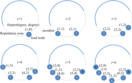
Figure 1: An illustration of an evolutionary research team. At each time, a new player joins the research team, and the group of the players with white numbers forms a hyperedge. It illustrates an usual scene: A new coming player $6$ wants to complete a work and write it as a paper. Suppose completing the paper needs four players. Then player $6$ would ask the leader $1$ for help, and the leader would suggest team members $2$ and $3$, who have most similar interest to player $6$, to cooperate.

A cooperative game consists of two elements: a set of players $N$ and a characteristic function specifying the value (benefit-minus-cost) created by subsets of players in the game. The characteristic function is a function $v$ mapping each subset $S$ of $N$ to the value $v(S)$ it creates. Regard nodes as players $N=\{i_{1},...,i_{n}\}$. Think of player $i_{l}$ as a lead node with players $i_{l_{1}},...,i_{l_{m}}$ as its research team members, and player $i_{c}$ as a candidate attempting to cooperate with $i_{l}$ and specific members (e. g. $i_{l_{1}},...,i_{l_{s}}$). Assume that the cooperation cost is $d(i_{l},i_{l_{1}},...,i_{l_{s}},i_{c})$, and suppose that those players will receive a benefit valued by $i_{l}$’s reputation $r(i_{l})$. We can define an intuitive characteristic function $v$ for this game as follows:

$$v(S)=\left\{\begin{aligned} r(i_{l})-d(i_{l},i_{l_{1}},...,i_{l_{s}},i_{c}),~{}~{}~{}{S=\{i_{l},i_{l_{1}},...,i_{l_{s}},i_{c}\};}\\ 0,~{}~{}~{}~{}~{}~{}~{}~{}~{}~{}~{}~{}~{}~{}~{}~{}~{}~{}~{}~{}~{}~{}~{}~{}~{}~{}~{}~{}~{}~{}~{}~{}~{}~{}{S\neq\{i_{l},i_{l_{1}},...,i_{l_{s}},i_{c}\}.}\end{aligned}\right.$$ (1)

Under the definition (1), if $v(\{i_{l},i_{l_{1}},...,i_{l_{s}},i_{c}\})>0$, those players will collaborate.

The empirical distributions of paper team sizes emerge a hook head and a fat tail, which means the sizes of substantial papers are around their average, and a few papers have a significantly large size. In reality, researchers in a small research team are more likely to write papers together. Members of a large research team rarely coauthor a paper all together, but rather with a fraction of members. Treating paper team size as a random variable $x$, we design a mechanism to simulate the distribution of $x$. Give the upper bound of small research team $\mu>0$, and the lower bound of large research team $\nu>0$. Denote the expected value of paper team size and the size of corresponding research team to be $\eta$ and $\lambda$ respectively. Let $\eta=\lambda$, if $\lambda\leq\mu$; Let $\eta=\mu$, if $\mu<\lambda\leq\nu$; Draw $\eta$ from a power law distribution with an exponent $\gamma$ and domain $[\mu,\lambda]$, if $\lambda>\nu$. Then draw $x$ from a Poisson distribution with expected value $\eta$. Note that in the description of the above game, $x=s+2$ and $\lambda=m+2$.

Cooperation costs could be considered as investments of time and effort to complete a study by crossing the distance between the research interest of the leader and that of the candidate, etc. Denote the spatio-temporal coordinates of player $i\in N$ by $(\theta_{i},t_{i})$, and write the player as $i(\theta_{i},t_{i})$. We abstractly geometrize the cost $d(i_{l},i_{l_{1}}...,i_{l_{s}},i_{c})=\pi-|\pi-|\theta_{i_{l}}-\theta_{i_{c}}||$, namely the angular distance between $i_{l}(\theta_{i_{l}},t_{i_{l}})$ and $i_{c}(\theta_{i_{c}},t_{i_{c}})$.

We now show how to value reputation. Considering the inefficient information of new players, we simply assume each lead node has the same attraction to new players and so value the reputation of a lead node $i(\theta_{i},t_{i})$ as $r(i)\propto 1/t_{i}$. Hence the expected number of $i$’s collaborators $k_{i}(t)=\alpha(T-t_{i})/t_{i}\approx\alpha T/t_{i}$ at time $T\gg t_{i}$, where $\alpha>0$. Those yield $P(k_{i}(T)<k)=P(t_{i}>\alpha T/k)$. The probability density of a lead node generated at $t_{i}$ is $1/T$. Hence $P(t_{i}>\alpha t/k)=1-P(t_{i}\leqslant\alpha T/k)=1-\alpha/k$. Then the tail of degree distribution $P(k)=\partial P(k_{i}(T)<k)/\partial k\propto 1/k^{2}$. We can obtain the general case $P(k)\propto 1/k^{1+1/\beta}$ for large enough $k$ by valuing the reputation $r(i)={\alpha}t^{-\beta}_{i}t^{\beta-1}$, where $\beta\in(0,1]$. The strict mathematical deduction of the degree distribution tail needs averaging on Poisson distribution, which is inspired by some of the same general ideas as explored in Ref. [25].

We next show how to generate a paper team, namely cooperation rule. Empirical collaboration behaviors have specific certainty (due to kin selection, network selection, etc.), as well as uncertainty. Consider an usual scene, a researcher $i$ of leader $j$’s research team wants to complete a work and write it as a paper, which needs $x\geq 2$ researchers to work together. Then $i$ would ask the leader $j$ for help, and $j$ would suggest $(\min(x,|R_{j}|)-2)$ members of his research team $R_{j}$, who have most similar interest to $i$, to cooperate with $i$. Such behavior can be viewed as kin selection, and is featured in certainty. When finishing the work is beyond the ability of the team $R_{j}$, the researcher $i$ would ask for external helpers. Uncertainty exists in this selection behavior, which inspires the design of randomly choosing $(x-\min(x,|R_{j}|)$ players outside of $R_{j}$ to cooperate. The uncertainty shorts the average shortest path length of modelled networks. Note that a researcher could belong to several research teams, hence above scene would happen in each team.

Based on above set-up, we build the hypergraph model as follows:

1.

Reputation assignment

For time $t=1,...,T\in\mathbb{Z}^{+}$ do:

Sprinkle nodes $N_{t}$ as new players uniformly and randomly on $S^{1}$. Select subset $N^{l}_{t}$ from $N_{t}$ randomly as lead nodes, and value the reputation of $j(\theta_{j},t_{j})\in N^{l}_{t}$ as $r(j)={\alpha}t^{-\beta}_{j}t^{\beta-1}$.

2.

Cooperation rule

For time $t=1,...,T$ do:

For each new node $i(\theta_{i},t_{i})\in N_{t}$, select a lead node set $M^{l}_{i}$ for which $\forall j(\theta_{j},t_{j})\in M^{l}_{i}$ satisfies $r(j)>\pi-|\pi-|\theta_{i}-\theta_{j}||$ and $t_{j}<t_{i}$. For each $j\in M^{l}_{i}$, add $i$ to $j$’s research team $R_{j}$, and generate a hyperedge at probability $p$ by grouping $i$, $j$, $(\min(x,|R_{j}|)-2)$ players of $R_{j}$ nearest to $i$, and $(x-\min(x,|R_{j}|))$ players $\not\in R_{j}$ randomly, where $x$ is the random variable above defined.

The player set of the model $N=\bigcup^{T}_{t=1}N_{t}$, and the number of players $n=|N|=\sum^{T}_{t=1}|N_{t}|$. Here we let $|N_{t}|$ and $|N^{l}_{t}|$ be constants over $t$. Compare with the model in Ref. [38], the new model reduces the number of parameters. Moreover, the new model has the ability to reproduce the empirical feature of the distribution of hyperdegrees, and that of paper team sizes. A node’s hyperdegree is the number of hyperedges that contain the node.

The data

To test the fitting ability of the proposed model, we analyze two empirical coauthorship networks (Table 1). Dataset PNAS is composed of 52,803 papers published in Proceedings of the National Academy of Sciences during 1999–2013. Dataset PRE comprises 24,079 papers published in Physical Review E during 2007-2016. Note that 43,304 papers of the first dataset belong to biological sciences, and the second dataset comes from physical sciences. The different collaboration level (reflected by the average number of authors per paper) of the two datasets (PNAS 6.028, PRE 3.102) helps to test the flexibility of the model.

In the process of extracting networks from those metadata, authors are identified by their names on their papers. For example, the author named “Carlo M. Croce” on his paper is represented by the name. We mainly focus on the distribution of degree and that of hyperdegree as well as some properties based on degrees. From the analysis of Ref. [39], we find that identifying authors by their name on papers holds the degree distribution feature of ground truth data, which partially verifies the reliability of the empirical networks used here.

Using surname and the initial of the first given name generates a lot of merging errors of name disambiguation[40]. Hence we compute the proportion of those authors, and that of those authors further conditioned on publishing more than one paper. Meanwhile, Chinese names were also found to account for the repetition of names[39]. We count the proportion of names with a given name less than six characters and a surname among major 100 Chinese surnames. The small proportions of such authors and those of such authors publishing more than one paper (Table 1) limit the impact of name repetition, especially for dataset PNAS.

Table 1: Specific statistical indexes of the empirical data.

Data	$a$	$b$	$c$	$d$
PNAS	2.62%	1.08%	2.90%	0.27%
PRE	3.85%	1.58%	19.2%	6.45%

Indexes $a$ and $b$ are the percent of authors who have a surname among major 100 Chinese surnames and only one given name shorter than six characters, and the percent of those authors further conditioned on publishing more than one papers respectively. Indexes $c$ and $d$ are the percent of authors who use surname and the initial of the first given name, and the percent of those authors further conditioned on publishing more than one papers respectively.

To reproduce specific features of the empirical data, we choose proper parameters (Table 2) to generate two hypergraphs, and extract simple graphs from them (where edges are formed between every two nodes in each hyperedge, isolated nodes are ignored, and multiple edges are viewed as one). Since the model is stochastic, we generate 20 networks with the same parameters, and compare their statistical indicators in Table 3. The finding is that the model is robust on those indicators (Table 4).

Table 2: The parameters of Synthetic-1, -2.

$T=5,000,6,000$	$N_{1}=100,15$	$N_{2}=5,5$	$p=0.25,0.4$
$\alpha=0.13,0.2$	$\beta=0.52,0.55$	$\gamma=4.2,4.2$	$\mu=6,2$	$\nu=42,6$

The parameters in the first row control network size, and those in the second row control a range of distributions, such as degree distribution, hyperdegree distribution, etc.

Table 3: Specific statistical indexes of the analyzed networks.

Network	NN	NE	GCC	AC	AP	MO	PG
PNAS	201,748	1,225,176	0.881	0.230	6.422	0.884	0.868
Synthetic-1	128,749	694,769	0.864	0.229	11.35	0.987	0.648
PRE	37,528	90,711	0.838	0.394	6.060	0.950	0.583
Synthetic-2	29,397	62,834	0.829	0.174	12.91	0.983	0.505

The indexes are the numbers of nodes (NN) and edges (NE), global clustering coefficient (GCC), assortativity coefficient (AC), average shortest path length (AP), modularity (MO), and the node proportion of the giant component (PG). The values of AP of the first two networks are calculated by sampling 300,000 pairs of nodes.

Table 4: The means and standard deviations (SDs) of specific indexes.

Synthetic-1	NN	NE	AC	GCC	PG	MO	AP
Mean	1.29E$+05$	6.23E$+04$	2.45E$-01$	8.64E$-01$	6.53E$-01$	9.87E$-01$	1.12E$+01$
SD	7.66E$+02$	1.14E$+04$	3.45E$-02$	7.08E$-04$	8.03E$-03$	4.97E$-04$	1.47E$-01$
Synthetic-2
Mean	2.93E$+04$	6.23E$+04$	1.35E$-01$	8.30E$-01$	5.06E$-01$	9.82E$-01$	1.22E$+01$
SD	1.48E$+02$	5.89E$+02$	2.93E$-02$	6.13E$-04$	6.48E$-03$	6.18E$-04$	5.33E$-01$

The meanings of headers are shown in the notes of Table 3.

Cooperation cost and reputation benefit

Based on the cost and the benefit of collaborations, we explain the distribution feature of paper team sizes. The benefit of joining a paper team is limited. The law of diminishing marginal utility holds in academic society. The allocation of academic achievements is often according to author order. Hence only the researchers with positive benefit-minus-cost would join the paper team. Assume the number of those researchers is $n_{r}$. Meanwhile, the joining behaviour has certain degrees of randomness. Let the joining probability be $p$. Then the paper team size will follow a binomial distribution, and so a Poisson distribution with expected value $n_{r}{p}$ approximately (Poisson limit theorem). Due to the law of diminishing marginal utility, the sizes of those papers would follow a generalized Poisson distribution, because this distribution describes situations where the occurrence probability of an event involves memory [41].

Some important works require many researchers (even from different research teams) work together, which would bring about huge economic and social benefits. The papers of those works would have many authors, and sometimes show their appearances in specific famous journals, e. g. a paper in Nature has 2,832 authors (see Fig. 3 in Ref.[34]). In fact, signing on a paper of a famous journal will also bring about a huge benefit. The existence of those papers leads to fat tails emerging paper team size distributions.

In brief, above analysis makes us think that benefit-minus-cost and the randomness of joining behaviour make a paper team size follow a generalized Poisson distribution, and huge expected benefits lead to fat-tail. There exists a cross-over between the two limits (Fig. 2). The fitting function of the distribution, including following discussed distribution of hyperdegree and that of degree, is a combination of a generalized Poisson distribution and a power-law function (Table 5). We perform a two-sample Kolmogorov-Smirnov (KS) test to compare the distributions of two data vectors: indexes (e. g. paper team sizes), the samples drawn from the corresponding fitting distribution. The null hypothesis is that the two data vectors are from the same distribution. The $p$-value of each fitting shows the test cannot reject the null hypothesis at the 5% significance level.

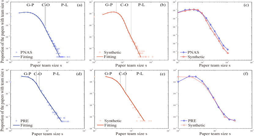
Figure 2: The distributions of sizes per paper team. In the panels of the first two columns, the regions “G-P”, “C-O”, “P-L” stand for generalized Poisson, cross-over and power-law respectively. The parameters and goodness of fittings are listed in Table 5.

Table 5: The parameters and goodness of fitting functions for degree distribution, hyperdegree distribution, and the distribution of paper team sizes, from the top down.

	$a$	$b$	$c$	$d$	$s$	$B$	$E$	$p$-value
	4.751	0.434	110.8	2.987	0.845	10	25	0.256
PNAS	0.085	0.367	2.368	2.941	11.99	3	7	0.128
	3.438	0.382	3,094	4.755	1.095	16	17	0.174
	5.082	0.380	708.4	3.580	0.898	13	32	0.074
Synthetic-1	0.664	0.365	16.15	3.694	1.999	4	9	0.971
	4.502	0.208	3,621	5.059	1.003	6	20	0.103
	2.776	0.156	8.910	2.758	0.898	5	6	0.118
PRE	0.038	0.399	4.260	3.079	25.56	3	10	0.875
	2.507	0.000	82.66	4.587	1.249	6	7	0.133
	2.352	0.2367	46.65	3.460	0.970	5	11	0.052
Synthetic-2	0.375	0.272	1.786	2.991	3.077	5	6	0.673
	2.007	0.065	116.1	4.756	1.146	5	7	0.887

The domains of generalized Poisson $f_{1}(x)={a(a+bx)^{x-1}}{\mathrm{e}^{-a-bx}/{x!}}$ , cross-over and power-law $f_{2}(x)=cx^{-d}$ are $[\min(x),E]$, $[B,E]$ and $[B,\max(x)]$ respectively. The fitting function defined on $[\min(x),\max(x)]$ is $f(x)=q(x)sf_{1}(x)+(1-q(x))f_{2}(x)$, where $q(x)=\mathrm{e}^{-(x-B)/(E-x)}$. The fitting processes are: Calculate parameters of $sf_{1}(x)$ and $f_{2}(x)$ by regressing the head and tail of empirical distribution respectively; Find $B$ and $E$ through exhaustion to make $f(x)$ pass KS test ($p$-value$>0.05$). The $p$-value measures the goodness-of-fit.

In the model, with a proper upper bound parameter $\mu$ (around average number of authors per paper of corresponding empirical data), the model can reproduce the generalized Poisson part of the distribution of paper team sizes, because most of modelled paper team sizes are drawn from Poisson distribution with an expected value around $\mu$. Meanwhile, with a proper lower bound parameter $\nu$, the mechanism can generate a few significantly large paper team sizes, and so the fat tails of the modelled paper team size distributions. We choose $\nu$ through iteration from the starting point of the power-law part in the corresponding empirical distribution of paper team sizes ($E$ in Table 5) until the modelled networks have the similar feature of the empirical distribution of degrees and that of paper team sizes.

Now we turn to explain the distribution feature of degrees. Substantial authors publish only one paper (PNAS: 64.8%, PRE: 63.9%), and most of paper team sizes draw from a generated Poisson distribution (PNAS: 99.9%, PRE: 99.9%). Those lead the generalized Poisson parts of degree distributions. Note that the boundaries of generated Poisson parts of paper team size distributions are 41 and 20 for PNAS and PRE respectively, which are detected by the boundary point detection algorithm for probability density functions in Ref.[38] (listed in Appendix).

With the growing of their papers, a few authors experience the cumulative process of collaborators over time, whose reputations also increase. As empirical data show, it is an accelerative process, which is often explained by cumulative advantage. The process reflects as the transition from a generated Poisson to a power-law (Fig. 3). Above explanation can also be used to explain the similar feature of hyperdegree distributions. Note that the nodes of large paper teams also have a large degree, which reflects as the outliers in the tails of degree distributions.

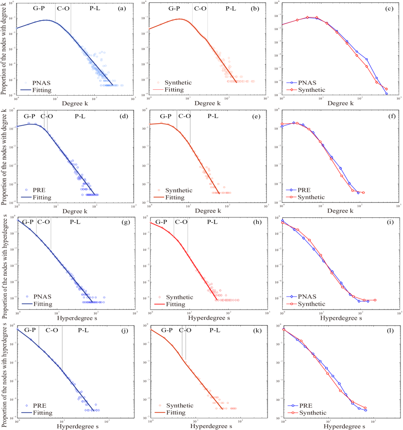
Figure 3: The empirical and synthetic distributions of collaborators/papers per author. The regions “G-P”, “C-O”, “P-L” stand for generalized Poisson, cross-over and power-law respectively. The parameters and goodness of fittings are listed in Table 5.

In the model, we can choose suitable parameters $\alpha$, $|N_{t}|$, $|N^{l}_{t}|$ and $p$ to make the hyperdegrees of substantial players be one (Synthetic-1: 48.5%, Synthetic-2: 61.5%). Meanwhile, the substantial modelled paper team sizes follow a generalized Poisson distribution (Synthetic-1: 99.9%, Synthetic-2: 100%). Those yield the generalized Poisson part of modelled degree distributions. The boundary of generalized Poisson part is 34 for Synthetic-1 and 23 for Synthetic-2. The mechanism of generating hyperedges makes only early lead nodes and specific players close to them can experience the cumulative process of connecting new players. The cumulative process generates the fat tails of modelled degree distributions, as well as those of modelled hyperdegree distributions (Fig. 3). The cumulative speed and so the power law exponent can be tuned by parameter $\beta$.

Spatial reciprocity and network reputation

Cooperation needs to be based on acquaintanceship. Hence there is an acquaintanceship network under each coauthorship network. Geographic contexts (such as organization, institution, etc.) contribute to emerging clustering structure in acquaintanceship network, namely “the friend of my friend is also my friend” [16]. The Internet extends the scope of acquaintanceship, which crosses spatial barriers even national boundaries. Therefore, the factor of clustering changes from geography to interest, namely “birds of a feather flock together”[42].

Cooperation costs make cooperators should have similar research interests, namely collaborations exist in researcher clusters formed by similar interests. Hence the spatial reciprocity principle in cooperative game theory[31] needs to be modified by interest in the situation of academic cooperation. In a network perspective, the extent of spatial reciprocity can be reflected by local clustering coefficient and the degree difference between a node and its neighbors.

Now we discuss the relationship between spatial reciprocity and network reputation. In the view of nodes, network reputation can be reflected by degree. Hence the relationship can be reflected by two functions of degree, namely the average local clustering coefficient of $k$-degree nodes $C(k)$, and the average degree of $k$-degree nodes’ neighbors $N(k)$. There is a transition in each of the functions (Fig. 4). The tipping points of $C(k)$ and $N(k)$ are detected by the boundary point detection algorithm for general functions in Ref.[38] (listed in Appendix). Inputs of the algorithm are $C(k)$/$N(k)$, $g(\cdot)=\log(\cdot)$ and $h(s)=a_{1}\mathrm{e}^{-((s-a_{2})/a_{3})^{2}}$/$h(s)=a_{1}s^{3}+a_{2}s^{2}+a_{3}s+a_{4}$ ($s$, $a_{i}\in{\mathbb{R}}$, $i=1,...,4$). Using those inputs is based on the observation of $C(k)$ and $N(k)$.

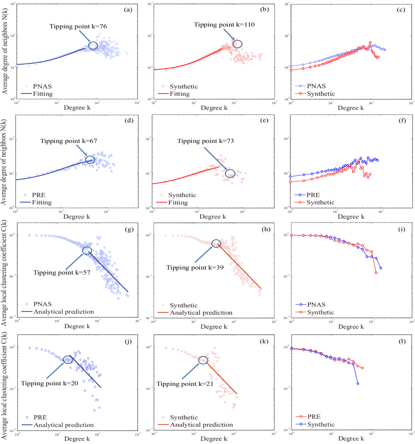
Figure 4: The relation between degree and average degree of neighbors, and that between local clustering coefficient and degree. The panels show $k$-degree nodes’ average degree of their neighbors and their the average local clustering coefficient respectively.

Coauthorship networks are found to have two features: high clustering (a high probability of a node s two neighbors connecting) and degree assortativity (a positive correlation coefficient between two random variables: a node’s degree and the average degree of the node’s neighbors), which are measured by GCC and AC in Table 3 respectively. To understand the essence of high clustering, degree assortativity, as well as the transitions in $C(k)$ and $N(k)$, we analyze the feature of the basic context of collaborations, i. e. research teams. Given the cost and benefit of joining a research team, only the researchers with positive benefit-minus-cost would join the team with a probability (that would be affected by previous members due to gossips, etc.). With an argument similar to the one used in the distribution of paper team sizes, we can assume the research team sizes follow a generalized Poisson distribution. A few research teams with a huge reputation would attract substantial collaborators and become significantly large ones.

Based on the above analysis, we can think that small degree authors comprises two parts: one is composed of the authors of small research teams, and other one comprises the unproductive authors belonging to small paper teams and to large research teams. Researchers in the small research team probably write a paper together, which causes they have a high local clustering coefficient, and a slight degree difference between them and their neighbors. Many authors in large research teams only write one paper, and the paper team only contains a few leaders. Hence those authors would have a relatively high local clustering coefficient, and a relatively small difference between their degree and the average degree of their neighbors. From above analysis, we can infer small degree authors contribute to degree assortativity and high clustering of coauthorship networks, which fits the empirical data (Figs. 4).

The collaborators of some productive authors may not coauthor, and some productive authors often have many collaborators. The degree difference emerges between those authors and their neighbors, on average. Hence we can infer those large degree authors negatively contribute to degree assortativity and high clustering. The inference fits the empirical data: the tails of $C(k)$ and $N(k)$ of each empirical network emerge a different trend from the heads (Figs. 4). Note that the authors of large paper teams also have a large degree, but contribute to degree assortativity and high clustering. The existence of those authors causes the scattered points of the tails of $C(k)$ and $N(k)$.

The model can generate research teams with a size distribution as above inferred. Due to the power function of reputation, the expected size $\mathbb{E}\lambda(T)$ of a research team of lead $i$ is proportional to $\sum^{T}_{s=t_{i}+1}{\alpha}t^{-\beta}_{i}s^{\beta-1}\approx{\alpha}(T/t_{i})^{\beta}$ for $T\gg t_{i}$. This yields $P(\mathbb{E}\lambda(T)<\kappa)=P(t_{i}>(\alpha/\kappa)^{1/\beta}T)$. With an argument similar for the reasonability of reputation function, we can obtain the tail of the distribution of modelled research team sizes $P(\kappa)=\partial P(\mathbb{E}\lambda_{i}(T)<\kappa)/\partial\kappa\propto 1/\kappa^{1+1/\beta}$. When $T\not\gg t_{i}$, the research team size $\lambda$ is drawn from a Poisson distribution with an expected value proper to ${\alpha}(T/t_{i})^{\beta}$ due to the Poisson point process of generating nodes. Hence the small modelled research team sizes are drawn from a range of Poisson distributions with expected values taking from a power function. With proper parameters, those can be used as basis to fit a given generalized Poisson distribution.

Most modelled hyperedges are generated by grouping a small fraction (around $\mu$) of nodes close in space, which expresses the spatial reciprocity principle. Moreover, to fit empirical hyperdegree distributions, we choose specific parameters make a large fraction of nodes only belong to one hyperedge. Meanwhile, most modelled hyperedges contain one lead node, and only early lead nodes and a few nodes close to them can be persistently contained by new hyperedges. Those yield that the small/large degree nodes contribute positively/negatively to degree assortativity and high clustering. Hence the model well reproduces the transitions. In addition, the tails of $C(k)$ proportional to $1/k$ also holds in modelled networks. For a lead node $i$, the probability of its new team member coauthor with the formers is $P=\int\alpha\mu t^{\beta}_{i}/t^{\beta}dt\propto t^{\beta}_{i}\propto 1/k_{i}$, where $k_{i}$ is the degree of node $i$.

Discussions and conclusions

Five typical mechanisms of cooperation evolution hold for academic collaborations, which inspires us to explore game mechanisms in the evolution of coauthorship networks. We define a cooperative game model on a circle, and reveal how the costs and benefits of individuals generate a range of statistical and topological features of coauthorship networks, such as fat-tail, small-world, etc. It overcomes the weakness of the model in Ref. [27], a lot of parameters, and has the new ability to fit the distribution of paper team sizes and that of hyperdegree. Moreover, it has the potential to illuminate specific views and implications in the broader study of cooperative behaviors as follows.

Do there exist innate rules behind the social complexity? It provides an example of how individual strategies based on maximizing benefit-minus-cost and on specific randomness generate the complexity emerged in coauthorship networks. The general idea of the model potentially bridges cooperative game theory and specific social networks generated by human strategies, e. g. social affiliation networks.

Does utilitarianism help the development of sciences? The strategy of maximizing benefit-minus-cost will give rise to flocking to famous research team or to hot fields. Taking such strategy helps to collect publications and citations, but suppresses diversity, and consequently does harm to the flexibility of academic environment. However, current academic evaluation methods and funding mechanisms are mainly oriented by specific indexes, e. g. the number of citations. Specific regulations could be simulated through the model to work out a way to maintain the balance in academic environment, while encouraging breakthroughs in key fields.

Authors’ contributions

The authors have contributed equally to this work. All authors conceived and designed the research. ZX, JPL and ML wrote the paper. ZX analyzed the data. All authors discussed the research and approved the final version of the manuscript.

Appendix

Detecting boundary points.

The following boundary detection algorithms come from Ref. [38].

Table 6: A boundary detection algorithm for probability density functions.

Input: Observations $D_{s}$, $s=1,...,n$, rescaling function $g(\cdot)$, and fitting model $h(\cdot)$.
For $k$ from $1$ to $\max(D_{1},...,D_{n})$ do:
Fit $h(\cdot)$ to the PDF $h_{0}(\cdot)$ of $\{D_{s},s=1,...,n|D_{s}\leq k\}$ by maximum-likelihood
estimation;
Do KS test for two data $g(h(t))$ and $g(h_{0}(t))$, $t=1,...,k$
with the null hypothesis they coming from the same continuous distribution;
Break if the test rejects the null hypothesis at significance level $5\%$.
Output: The current $k$ as the boundary point.

Table 7: Boundary point detection algorithm for general functions.

Input: Data vector $h_{0}(s)$, $s=1,...,K$, rescaling funtion $g(\cdot)$, and fitting model $h(\cdot)$.
For $k$ from $1$ to $K$ do:
Fit $h(\cdot)$ to $h_{0}(s)$, $s=1,...,k$ by regression;
Do KS test for two data vectors $g(h(s))$ and $g(h_{0}(s))$, $s=1,...,k$ with the null
hypothesis they coming from the same continuous distribution;
Break if the test rejects the null hypothesis at significance level $5\%$.
Output: The current $k$ as the boundary point.

References

- 1. Börner K, et al. (2010) A multi-level systems perspective for the science of team science. Sci Transl Med 2(49): 49cm24
- 2. Jones BF, Wuchty S, Uzzi B (2008) Multi-university research teams: Shifting impact, geography, and stratification in science. Science 322(5905): 1259-1262.
- 3. Adams J (2012) Collaborations: The rise of research networks. Nature 490: 335-336.
- 4. Shrum W, Genuth J, Chompalov I (2007) Structures of Scientific Collaboration (MIT, Cambridge, MA)
- 5. Uzzi B, Mukherjee S, Stringer M, Jones B (2013) Atypical combinations and scientific impact. Science 342(6157): 468-472.
- 6. Wuchty S, Jones BF, Uzzi B (2007) The increasing dominance of teams in production of knowledge. Science 316(5827): 1036-1039.
- 7. Glänzel W, Schubert A (2004) Analysing scientific networks through co-authorship. Handbook of quantitative science and technology research 11: 257-276.
- 8. Glänzel W (2014) Analysis of co-authorship patterns at the individual level. Transinformacao 26: 229-238.
- 9. Sarigöl E, Pfitzner R, Scholtes I, Garas A, Schweitzer F (2014) Predicting scientific success based on coauthorship networks. EPJ Data Science 3(1): 1-16.
- 10. Mali F, Kronegger L, Doreian P, Ferligoj A, Dynamic scientific coauthorship networks (2012) In: Scharnhorst A, Börner K, Besselaar PVD editors. Models of science dynamics. Springer. pp. 195-232.
- 11. Jia T, Wang D, Szymanski BK (2017) Quantifying patterns of research-interest evolution. Nature Human Behaviour 1: 0078.
- 12. Newman M (2001) Scientific collaboration networks. I. network construction and fundamental results. Phys Rev E 64: 016131.
- 13. Newman M (2001) Scientific collaboration networks. II. shortest paths, weighted networks, and centrality. Phys Rev E 64: 016132.
- 14. Newman M (2001) The structure of scientific collaboration networks. Proc Natl Acad Sci USA 98: 404-409.
- 15. Newman M (2004) Coauthorship networks and patterns of scientific collaboration. Proc Natl Acad Sci USA 101: 5200-5205.
- 16. Newman M (2002) Assortative mixing in networks. Phys Rev Lett 89: 208701.
- 17. Xie Z, Li M, Li JP, Duan XJ, Ouyang ZZ (2018) Feature analysis of multidisciplinary scientific collaboration patterns based on pnas. EPJ Data Science 7: 5.
- 18. Barabási AL, Jeong H, Néda Z, Ravasz E, Schubert A, Vicsek T. (2002) Evolution of the social network of scientific collaborations. Physica A 311: 590-614.
- 19. Moody J (2004) The strucutre of a social science collaboration network: disciplinery cohesion form 1963 to 1999. Am Sociol Rev 69(2): 213-238.
- 20. Perc C (2010) Growth and structure of Slovenia’s scientific collaboration network. J Informetr 4: 475-482.
- 21. Wagner CS, Leydesdorff L (2005) Network structure, self-organization, and the growth of international collaboration in science. Res Policy 34(10): 1608-1618.
- 22. Tomassini M, Luthi L (2007) Empirical analysis of the evolution of a scientific collaboration network. Physica A 285: 750-764.
- 23. Santos FC, Pacheco JM (2005) Scale-free networks provide a unifying framework for the emergence of cooperation. Phys Rev Lett 95(9): 098104.
- 24. Catanzaro M, Caldarelli G, Pietronero L (2004) Assortative model for social networks. Phys Rev E 70: 037101.
- 25. Krioukov D, Kitsak M, Sinkovits RS, Rideout D, Meyer D, Boguá M (2012) Network cosmology. Sci Rep 2: 793.
- 26. Xie Z, Rogers T (2016) Scale-invariant geometric random graphs. Phys Rev E 93: 032310.
- 27. Xie Z, Ouyang ZZ, Li JP (2016) A geometric graph model for coauthorship networks. J Informetr 10: 299-311.
- 28. Pennisi E (2005) How did cooperative behavior evolve? Science 309(5731): 93-93.
- 29. Nowak MA (2006) Five rules for the evolution of cooperation. Science 314(5805): 1560-3.
- 30. Hoekman J, Frenken K, Tijssen RJW (2010) Research collaboration at a distance: Changing spatial patterns of scientific collaboration within Europe. Res Policy 39: 662-673.
- 31. Hauert C, Doebeli M (2004) Spatial structure often inhibits the evolution of cooperation in the snowdrift game. Nature 428(6983): 643-6.
- 32. Milojević S (2014) Principles of scientific research team formation and evolution. Proc Natl Acad Sci USA 111: 3984-3989.
- 33. Börner K, Maru JT, Goldstone RL (2004) The simultaneous evolution of author and paper networks. Proc Natl Acad Sci USA 101(suppl 1), 5266-5273.
- 34. Xie Z, Xie ZL, Li M, Li JP, Yi DY (2017) Modeling the coevolution between citations and coauthorship of scientific papers. Scientometrics 112: 483-507.
- 35. Goldschmidt C (2005) Critical random hypergraphs: the emergence of a giant set of identifiable vertices. Ann Probab 33(4), 1573-1600.
- 36. Estrada E, Rodríguez-Velázquez JA (2006) Subgraph centrality and clustering in complex hyper-networks. Physica A 364, 581-594.
- 37. Darling RW, Norris JR (2005) Structure of large random hypergraphs. Ann Appl Probab, 15(1A), 125-152.
- 38. Xie Z, Ouyang ZZ, Li JP, Dong EM, Yi DY (2018) Modelling transition phenomena of scientific coauthorship networks. J Assoc Inf Sci Technol 69(2): 305-317.
- 39. Kim J, Diesner J (2016) Distortive effects of initial-based name disambiguation on measurements of large-scale coauthorship networks. J Assoc Inf Sci Technol 67(6): 1446-1461.
- 40. Milojević S (2010) Modes of collaboration in modern science-beyond power laws and preferential attachment. J Assoc Inf Sci Technol 61(7): 1410-1423.
- 41. Consul PC, Jain GC (1973) A generalization of the Poisson distribution. Technometrics 15(4): 791-799.
- 42. McPherson M, Smith-Lovin L, Cook JM (2001) Birds of a feather: homophily in social networks. Annu Rev Sociol 27(1): 415-444.