A class of simple bouncing and late-time accelerating cosmologies in $f(R)$ gravity

Abstract

We consider the field equations for a flat FRW cosmological model, in a generic $f(R)$ gravity model and cast them into a, completely normalized-dimensionless, system of O.D.Es for the scale factor and the function $f(R)$, with respect to the scalar curvature $R$. It is shown that under reasonable assumptions one can produce simple analytical and numerical solutions describing bouncing cosmological models where in addition there are late-time accelerating. Possibility of extending these results is briefly discussed.

PACS numbers: 11.25.Pm

1 Introduction

Extended theories of gravity, alternate to Einstein’s General Relativity (GR), were proposed to solve the problem of the standard cosmological model of GR and also in relation to the quantization of gravity (see e.g. [1]-[4]). Today the standard cosmological model (SCM) also called the Big-Bang cosmology is the most acceptable model of the Universe up to this day. Among its major successes is the Hubble law for the expansion of the Universe, the black body nature of the cosmic microwave background (CMB) radiation and the light element abundances predicted by it (see e.g. [5] and references therein). However the SCM includes a number of deficiencies such as the problems of magnetic monopoles, gravitons and baryon asymmetry. Also despite its success in describing the observable Universe up to a hundredth of a second after its initial moment, there exist unanswered questions regarding the initial state of it, namely the horizon and flatness problems [6].

Though the inflation concept has been introduced to solve the above problems of the SCM, it suffers also from another major unresolved problem, namely the existence of the initial cosmological singularity, predicted by standard singularity theorems [7]. A singular initial state is usually an extreme situation where physical observable quantities such as temperature, mass-energy density and curvature attain infinite values, a case which signifies the breakdown of the underlying physical theory. Attempts to remedy this situation include, among others, consideration of cosmological models where in fact at the initial moment (usually taken to be $t=0$) there exist finite values for the physical quantities and in particular for the scale factor $a(t)$ of the evolution of the Universe and the scalar curvature $R$. These are the so-called bouncing cosmological models, where presumably the Universe undergoes a previous contracting phase in its evolution.

There exists a vast literature on bouncing cosmological models, mainly in the frame of extended theories of gravity, where the GR action is replaced by a generic function of the scalar curvature $f(R)$. A very incomplete list includes the following: Bouncing cosmological models in the frame of $f(R)$ gravity and bi-gravity appeared in [8]. Bouncing cosmological models from higher powers of gravity appeared in [9]. Static Einstein models in power-law form of the action, namely in $f(R)$ gravity appeared in [10]. Bouncing cosmological models in Palatini $f(R)$ gravity appeared in [11], and also in [12]. Bouncing cosmological models in $F(R,\phi)$ gravity with phantom equation of state (EoS) appeared in [13]. Isotropic and anisotropic bouncing cosmological models in Palatini $f(R)$ gravity appeared in [14]. Bouncing cosmology from Lagrange-multiplier modified gravity appeared in [15], while an interesting review of the Palatini approach to modified gravity such as the case of $f(R)$ gravity appeared in [16]. Bouncing cosmological models in the $f(R)$-Palatini variational formalism appeared in [17], while $f(R,T)-$gravity and its various phenomena and cosmological models appeared in [18]. Bouncing cosmological models in the frame of Horava-Lifshitz $f(R)$ gravity appeared in [19], while bouncing and late-time accelerating cosmological models, in the Born-Infeld-like $f(R)$ gravity appeared in [20].

According to recent cosmological observations in terms of Supernovae Ia, large scale structure with the baryon acoustic oscillations, cosmic microwave background radiation and weak lensing, the current expansion of the universe is accelerating (see e.g. the introduction of [8] and references therein). In this context, cosmological models that attempt to incorporate both the early stage bouncing behavior with late time accelerating phase were vastly considered in the literature. An incomplete list includes e.g. [21]-[43] and references therein. In this paper we consider the field equations for an $f(R)$ cosmology with metric described by Eq. (5), as they appear in e.g. [1]. We use an approach that, to the author’s knowledge, has not been explicitly followed in the relevant literature. This consists of the assumption that we have a bouncing cosmological model where the scalar curvature increases monotonically, as we approach the initial moment $t=0$, in the contracting phase of the Universe. This solution is then matched to its mirror-symmetric, with respect to the time $t$, for the expanding phase of the Universe. By a direct calculation the field equations are transformed to a system consisting of a first order equation for the metric and a second order equation for the function $f(R)$, with respect to the scalar curvature $R$. These are then solved analytically, for some simple ansatze and numerically also, resulting in bouncing cosmological models with late-time acceleration.

This paper is organized as follows: In section 2 we provide the general setting, for an $f(R)$ cosmology, along with the field equations describing it. In section 3 we explicitly give our ansatz and assumptions. In section 4 we reduce the field equations to a completely normalized-dimensionless system of O.D.Es for the scale factor of the metric and the function $f(R)$ and we provide the class of simple analytical models that are proposed. In section 5 we give an example of a cosmological model from a numerical treatment of the above system. In section 6 we explain and justify our construction regarding its smoothness, as a solution to the field equations. Finally in section 7 we give a brief discussion of the results.

2 The Setting

We consider the $f(R)-$gravity action, with matter content [5]

$$S=S_{g}+S^{(m)}=\int d^{4}x\sqrt{-g}\left[\frac{1}{2\kappa^{2}}f(R)+L^{(m)}\right]$$ (1)

where $\kappa^{2}=8\pi G$ and we use geometrical units by setting $c=G=1$. The stress-energy tensor is given by [5]

$$T_{\mu\nu}:=\frac{-2}{\sqrt{-g}}\frac{\delta[\sqrt{-g}L^{(m)}]}{\delta g^{\mu\nu}}$$ (2)

Varying with respect to $g^{\mu\nu}$ we obtain the field equations [1]

$$f^{{}^{\prime}}(R)R_{\mu\nu}-\frac{f(R)}{2}g_{\mu\nu}=\nabla_{\mu}\nabla_{\nu}f^{{}^{\prime}}(R)-g_{\mu\nu}\Box f^{{}^{\prime}}(R)+\kappa^{2}T_{\mu\nu}$$ (3)

where a prime denotes derivative with respect to the scalar curvature $R$ and we use the notation $\Box:=g^{\mu\nu}\nabla_{\mu}\nabla_{\nu}$. The trace of Eq. (3) gives [1]

$$3\Box f^{{}^{\prime}}(R)+Rf^{{}^{\prime}}(R)-2f(R)=\kappa^{2}T$$ (4)

where $T:=T^{\alpha}_{\alpha}:=g^{\mu\nu}T_{\mu\nu}$ is the trace of the stress-energy tensor. Thus Eq. (4) shows that $f^{{}^{\prime}}(R)$ is a dynamical-scalar degree of freedom of the theory.

We consider now a flat FRW metric

$$ds^{2}=-dt^{2}+a^{2}(t)[dx^{2}+dy^{2}+dz^{2}]$$ (5)

where $a(t)$ is the scale factor and $H:=\dot{a}/a$ is the Hubble parameter. The stress-energy conservation $\nabla_{\nu}T^{\mu\nu}=0$ is automatically satisfied by the field equations (3). The field equations become [1]

$$3H^{2} = \frac{\kappa^{2}}{f^{{}^{\prime}}(R)}\left[\rho^{(m)}+\frac{Rf^{{}^{\prime}}(R)-f(R)}{2}-3H\dot{R}f^{{}^{\prime\prime}}(R)\right]$$

$$2\dot{H}+3H^{2} = \frac{-\kappa^{2}}{f^{{}^{\prime}}(R)}\left[P^{(m)}+f^{{}^{\prime\prime\prime}}(R)(\dot{R})^{2}+2H\dot{R}f^{{}^{\prime\prime}}(R)+\right.$$ (6)

$$+ \left.\ddot{R}f^{{}^{\prime\prime}}(R)+\frac{f(R)-Rf^{{}^{\prime}}(R)}{2}\right]$$

namely the generalized Friedman and Raychaudhuri equations.

We use now a single perfect fluid with barotropic equation of state (EoS) of the form $P^{(m)}=w\rho^{(m)}$. Thus, with the sign conventions we adopt for the metric, we have

$$T^{\mu}_{\nu}=diag\left(-\rho^{(m)},P^{(m)},P^{(m)},P^{(m)}\right)$$ (7)

where $T=-\rho^{(m)}+3P^{(m)}=(3w-1)\rho^{(m)}$, while we also have

$$R=6\left(\frac{\ddot{a}}{a}+\frac{\dot{a}^{2}}{a^{2}}\right)=6(\dot{H}+2H^{2})$$ (8)

for the scalar curvature of the cosmological spacetime metric of Eq. (5). For the rest of this paper we will be considering pressureless dust, i.e. $w=0$ and from the stress-energy tensor conservation $\nabla_{\nu}T_{\mu}^{\nu}=0$, we obtain

$$\rho^{(m)}=\rho_{0}\left(\frac{a_{0}}{a}\right)^{3},\;\;\;T=-\rho^{(m)}$$ (9)

3 The model

We now write the field equations (2) as [5]

$$3H^{2} = \kappa^{2}\rho_{(eff)}$$ (10)

$$2\dot{H}+3H^{2} = -\kappa^{2}P_{(eff)}$$ (11)

where

$$\rho_{(eff)} = \frac{1}{f^{{}^{\prime}}(R)}\left[\rho^{(m)}+\frac{Rf^{{}^{\prime}}(R)-f(R)}{2}-3H\dot{R}f^{{}^{\prime\prime}}(R)\right]$$

$$P_{(eff)} = \frac{1}{f^{{}^{\prime}}(R)}\left[P^{(m)}+f^{{}^{\prime\prime\prime}}(R)(\dot{R})^{2}+2H\dot{R}f^{{}^{\prime\prime}}(R)+\right.$$ (12)

$$+ \left.\ddot{R}f^{{}^{\prime\prime}}(R)+\frac{f(R)-Rf^{{}^{\prime}}(R)}{2}\right]$$

Also we have $\Box:=g^{\mu\nu}\nabla_{\mu}\nabla_{\nu}=-\partial_{tt}-3H\partial_{t}$ and thus using Eqs. (3) one can easily compute that

$$\Box f^{{}^{\prime}}(R) = \left(P^{(m)}-\frac{1}{3}\rho^{(m)}\right)-f^{{}^{\prime}}(R)\left(P_{(eff)}-\frac{1}{3}\rho_{(eff)}\right)+$$ (13)

$$+ \frac{2}{3}\left[f(R)-Rf^{{}^{\prime}}(R)\right]$$

From Eqs. (10) we have

$$\dot{\rho}_{(eff)}=-3H(\rho_{(eff)}+P_{(eff)})\Longrightarrow P_{(eff)}=-\frac{\dot{\rho}_{(eff)}}{3H}+\rho_{(eff)}$$ (14)

Then Eq. (4) becomes

$$T+f^{{}^{\prime}}(R)\left[\frac{\dot{\rho}_{(eff)}}{H}+2\rho_{(eff)}\right]-Rf^{{}^{\prime}}(R)=\kappa^{2}T$$ (15)

and the first of Eqs. (10) becomes

$$f^{{}^{\prime}}(R)\left[3H^{2}-\frac{\kappa^{2}R}{2}+\frac{\kappa^{2}\rho^{{}^{\prime}}_{(eff)}}{2}\frac{a}{a^{{}^{\prime}}}\right]=\frac{1}{2}\kappa^{2}(\kappa^{2}-1)T$$ (16)

while we will be using Eq. (9) also.

We now seek for a bouncing cosmological model, so that for $t=0$ we demand that the scalar curvature is finite, $R(t=0):=R_{0}>0$ and moreover we must have $\dot{R}(t=0)=\dot{R}(R=R_{0})=0$. This indeed implies, from $\dot{a}=a^{{}^{\prime}}(R)\dot{R}$, that $\dot{a}(t=0)=0$, while in general $a^{{}^{\prime}}(R=R_{0})\neq 0$. Also $a_{0}:=a(t=0)=a(R=R_{0})>0$ must be finite. Moreover we seek for a late time accelerating cosmology. Thus for $t\longrightarrow\infty$ we must have $\dot{H}_{\infty}=0$ and thus $R\longrightarrow R_{\infty}=6(\dot{H}_{\infty}+2H_{\infty}^{2})=12H_{\infty}^{2}>0$. Then from Eq. (8) we obtain

$$\frac{d}{dR}\left[(\dot{R})^{2}\right]+2\left[\frac{a^{{}^{\prime\prime}}}{a}+\frac{a^{{}^{\prime}}}{a}\right](\dot{R})^{2}=\frac{Ra}{3a^{{}^{\prime}}}$$ (17)

with solution

$$(\dot{R})^{2}=\frac{1}{3(aa^{{}^{\prime}})^{2}}\int_{R_{0}}^{R}Ra^{3}a^{{}^{\prime}}(R)dR$$ (18)

Now we compute from Eq. (18), the term $3H^{2}$ and also use Eq. (9) into Eq. (16). We then take a derivative with respect to $R$, and also we assume, as stated previously, that the matter content of the Universe is in the form of pressureless dust, namely we set $w=0$. After some algebra we finally obtain

$$\left(\frac{a^{{}^{\prime}}}{a}\right) = \frac{\kappa^{2}(\kappa^{2}-1)\rho_{0}}{2Rf^{{}^{\prime}}(R)}\left(\frac{a_{0}}{a}\right)^{3}\left(\frac{a^{{}^{\prime}}}{a}\right)-\frac{\kappa^{2}(\kappa^{2}-1)\rho_{0}}{2[f^{{}^{\prime}}(R)]^{2}}\left(\frac{a_{0}}{a}\right)^{3}\frac{f^{{}^{\prime\prime}}(R)}{R}+$$ (19)

$$+ \frac{\kappa^{2}}{2R}+2\kappa^{2}\left(\frac{a^{{}^{\prime}}}{a}\right)-\frac{5\kappa^{2}\rho^{{}^{\prime}}_{(eff)}(R)}{2R}-\frac{\kappa^{2}}{2}\left(\frac{a}{a^{{}^{\prime}}}\right)\frac{\rho^{{}^{\prime\prime}}_{(eff)}}{R}+$$

$$+ \frac{\kappa^{2}}{2}\frac{\rho^{{}^{\prime}}_{(eff)}(R)}{R}\frac{aa^{{}^{\prime\prime}}}{(a^{{}^{\prime}})^{2}}$$

We now normalize the curvature with respect to $R_{0}$, namely we define the new variable $R_{n}:=R/R_{0},\;\;\;0<R_{n}\leq 1$. Also it is assumed from now on that a prime denotes derivative with respect to the new normalized variable for the curvature, namely $()^{{}^{\prime}}:=d()/dR_{n}$. Also we define $Y:=(a_{0}/a)^{3}$, $c_{0}:=\frac{\kappa^{2}}{2(2\kappa^{2}-1)}$, $R_{\rho}:=\kappa^{2}\rho_{0}/2$ and $c_{1}:=\frac{(\kappa^{2}-1)}{(2\kappa^{2}-1)}$. It is evident that $R_{\rho}$ is a measure (in units of curvature) of the mass-energy density of the Universe, at the moment of bouncing. Then we make our unique central assumption in this paper, that specifies the class of solutions that we seek to study, in the form of $\rho_{(eff)}:=\rho_{1}Y^{m}$ where $m,\;\rho_{1}$ are constants to be determined below, Eq. (19) becomes

$$Y^{{}^{\prime}}=\frac{3Y\left[c_{0}-\frac{c_{1}R_{\rho}}{f^{{}^{\prime}}(R_{n})}\frac{f^{{}^{\prime\prime}}}{f^{{}^{\prime}}}Y\right]}{R_{n}\left[1+\frac{c_{1}R_{\rho}}{R_{n}f^{{}^{\prime}}(R_{n})}Y\right]}$$ (20)

In terms of the above definitions Eq. (18) becomes

$$(\dot{R}_{n})^{2}=\frac{R_{0}Y^{10/3}}{(Y^{{}^{\prime}})^{2}}\int_{R_{n}}^{1}\frac{R_{n}Y^{{}^{\prime}}}{Y^{7/3}}dR_{n}:=\frac{R_{0}GY}{(Y^{{}^{\prime}})^{2}}$$

$$G:=G(R_{n},Y)=\frac{3}{4}Y^{7/3}\left[\frac{R_{n}}{Y^{4/3}}-1+\int_{R_{n}}^{1}\frac{dR_{n}}{Y^{4/3}}\right]$$ (21)

while from the first of Eqs. (2) and using our assumption $\rho_{(eff)}:=\rho_{1}Y^{m}$ we obtain

$$\rho_{0}Y+\frac{1}{2}[R_{n}f^{{}^{\prime}}(R_{n})-f(R_{n})]+\frac{Y^{{}^{\prime}}}{Y}\frac{(\dot{R}_{n})^{2}}{R_{0}}f^{{}^{\prime\prime}}(R_{n})=\frac{\rho_{1}}{R_{0}}f^{{}^{\prime}}(R_{n})Y^{m}$$ (22)

4 Reduction of the system and analytical treatment

In principle we would have the freedom to assume a quite general form for the $f(R)-$gravity models under study. For example we would assume that we have the following class of polynomial $f(R)-$gravity models, of the form

$$f(R)=-2\Lambda+f_{1}R+\frac{1}{2}\frac{f_{2}}{R_{0}}R^{2}+\frac{1}{3}\frac{f_{3}}{R_{0}^{2}}R^{3}$$ (23)

Here $\Lambda>0$ is the cosmological constant, $f_{1},\;f_{2},\;f_{3}$ are dimensionless constants and $R_{0}$ is the finite curvature scalar at the moment of bouncing, which may be taken to be of the order of the inverse square of the Planck length, namely

$$R_{0}\simeq\frac{1}{L_{pl}^{2}}\simeq 0.385\times 10^{70}m^{-2}$$ (24)

Also we can make an assumption for the order of magnitude estimate of

$$R_{\rho}=\frac{8\pi}{2}\frac{M_{pl}}{L_{pl}^{3}}\simeq 4.835\times 10^{70}m^{-2}$$ (25)

and $\lambda:=R_{\rho}/R_{0}\simeq 12.563$. The dimension of the function $f(R)$ in Eq. (23) is that of a scalar curvature, namely that of $R_{0}$, for example, so we define the completely dimensionless function $F(R_{n}):=f(R_{n})/R_{0}$ and Eq. (20) assumes its completely dimensionless-normalized form, suitable for numerical treatment, as follows

$$Y^{{}^{\prime}}=\frac{3Y\left[c_{0}-\frac{c_{1}\lambda}{F^{{}^{\prime}}(R_{n})}\frac{F^{{}^{\prime\prime}}}{F^{{}^{\prime}}}Y\right]}{R_{n}\left[1+\frac{c_{1}\lambda}{R_{n}F^{{}^{\prime}}(R_{n})}Y\right]}$$ (26)

where of course from above we obtain $\lambda\simeq 12.563$, $c_{0}=0.255$ and $c_{1}=0.49$, due to the fact that we have chosen units where $\kappa^{2}=8\pi$. Also we define the free dimensionless parameter $\mu:=\rho_{1}/R_{0}$. Then Eq. (22) assumes its completely dimensionless-normalized form as

$$\lambda Y+2\pi[R_{n}F^{{}^{\prime}}(R_{n})-F(R_{n})]+\frac{G}{Y^{{}^{\prime}}}F^{{}^{\prime\prime}}(R_{n})=\mu F^{{}^{\prime}}(R_{n})Y^{m}$$ (27)

Finally using Eqs. (26), (3) into Eq. (27) we obtain after some algebra, the completely dimensionless-normalized form for the evolution of the $f(R)-$gravity curvature function as

$$F^{{}^{\prime\prime}} = \frac{G_{1}}{G_{2}}$$

$$G_{2} := G_{2}(R_{n},Y,F,F^{{}^{\prime}})=GR_{n}\left[1+\frac{c_{1}\lambda}{R_{n}F^{{}^{\prime}}}Y\right]+$$

$$+ 3Y^{2}\frac{c_{1}\lambda}{(F^{{}^{\prime}})^{2}}\left[\mu F^{{}^{\prime}}Y^{m}-\lambda Y-2\pi[R_{n}F^{{}^{\prime}}-F]\right]$$

$$G_{1} := G_{1}(R_{n},Y,F,F^{{}^{\prime}})=3c_{0}Y\left[\mu F^{{}^{\prime}}Y^{m}-\lambda Y-2\pi[R_{n}F^{{}^{\prime}}-F]\right]$$ (28)

Thus we can numerically integrate Eqs. (26), (4), using also the last of Eqs. (3).

Now we study the Hubble parameter of these models. Regarding the Hubble parameter in our epoch, in the notation used here, it is given by [6]

$$H_{\infty}=72\pm 8Km/sec/Mpc$$ (29)

Assuming that the Universe in the present moment is accelerating we obtain $R_{\infty}=6(\dot{H}_{\infty}+2H_{\infty}^{2})=12H_{\infty}^{2}=0.726\times 10^{-39}m^{-2}$. When expressed in normalized-dimensionless units, with respect to the curvature constant $R_{0}$ of Eq. (24), it assumes the form

$${\cal R}_{\infty}:=\frac{R_{\infty}}{R_{0}}\simeq 1.885\times 10^{-109}$$ (30)

A careful calculation, using Eqs. (17), (3) yields

$$A:=1+\frac{\dot{H}}{H^{2}}=1+\frac{\left[1-\int_{R_{n}}^{1}\frac{dR_{n}}{Y^{4/3}}\right]}{2\left[\frac{R_{n}}{Y^{4/3}}-1+\int_{R_{n}}^{1}\frac{dR_{n}}{Y^{4/3}}\right]}$$ (31)

A sufficient condition for late time acceleration is that as $R_{n}\longrightarrow 0$ we have $A>0$.

We now present a class on exact, analytical, cosmological models which are bouncing at the origin of time $t=0$ (corresponding to $R_{n}=1$), and also are late-time accelerating. We assume the following form of the functions $Y,\;F$

$$Y := y_{0}R_{n}^{a_{1}}$$

$$F := f_{0}R_{n}^{a_{1}}$$ (32)

where $y_{0},\;f_{0},\;a_{1}$ are positive constants. Then from Eq. (26) we obtain

$$r:=\frac{y_{0}}{f_{0}}=\frac{3c_{0}-a_{1}}{c_{1}\lambda(3a_{1}-1)}$$ (33)

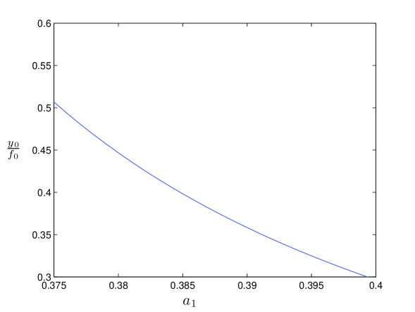
Figure 1: The function of Eq. (33), plotted against the permitted range of parameter values of $a_{1}$, given by Eq. (35).

This is plotted in Fig. 1, for the allowed parameter region of the constant $a_{1}$, to be determined below. We then substitute the first of Eqs. (4) into Eq. (31) and after a careful evaluation we find that in order to have late-time accelerating cosmologies, namely to have $A>0$ as $R_{n}\longrightarrow 0$ it is necessary that $\alpha_{1}>3/8$. Then we substitute the first of Eqs. (4) into the definition of the function $G$, of Eq. (3) and we choose to set

$$y_{0}^{4/3}:=\frac{1}{\left(1-\frac{4a_{1}}{3}\right)}>0$$ (34)

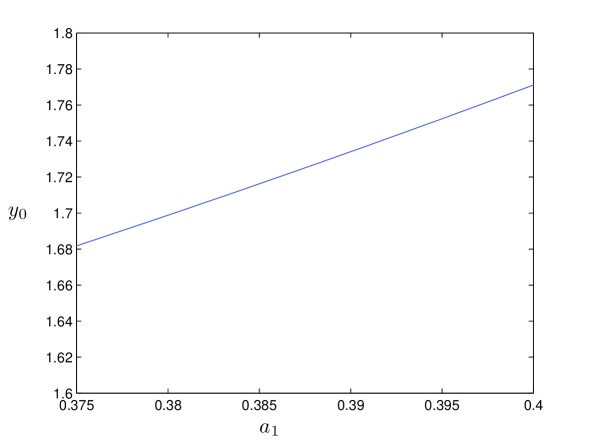
Figure 2: The function of Eq. (34), plotted against the permitted range of parameter values of $a_{1}$, given by Eq. (35).

This is plotted in Fig. 2, for the allowed parameter region of the constant $a_{1}$, to be determined below. From Eqs. (31), (34) we thus find that the range of permitted values of the constant $a_{1}$ is

$$\frac{3}{8}<a_{1}<\frac{3}{4}$$ (35)

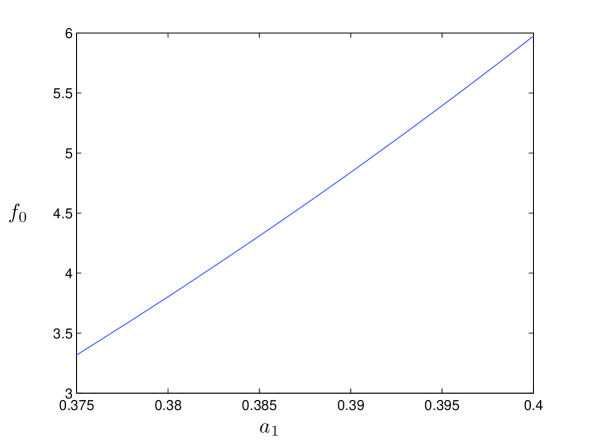
Figure 3: The constant $f_{0}$ of Eq. (4), plotted against the permitted range of parameter values of $a_{1}$, given by Eq. (35).

The constant $f_{0}$ is readily determined by the combination of Eqs. (33), (34) and it is plotted in Fig. 3. All the previous results are now substituted into Eq. (4). Also we assume that the constant $m=1/a_{1}$. We then find after some careful algebra that

$$3\mu\left[rc_{1}\lambda(a_{1}-1)-c_{0}a_{1}\right]y_{0}^{m}=a_{1}(a_{1}-1)(a_{1}+c_{1}\lambda r)+$$ (36)

$$+ \left[\frac{3rc_{1}\lambda(a_{1}-1)}{a_{1}}-3c_{0}\right]\left[\lambda r+2\pi(a_{1}-1)\right]$$

This determines the positive constant $\mu$ and it is plotted in Fig. 4. Thus Eqs. (4) constitute an exact analytic cosmological model for the range of the parameter $a_{1}$, given by Eq. (35). These are bouncing at the origin of time ($t=0$), as it will also be explained in Section 6, and are late-time accelerating. This model shows that one can obtain relatively easy, simple cosmological models with the aforementioned properties, in the frame of the $f(R)-$gravity theories. Using Eq. (30) into the first of Eqs. (4) we obtain

$$N:=ln\left(\frac{a_{\infty}}{a_{0}}\right)\simeq 251a_{1}$$ (37)

for the number of e-foldings from the initial moment of the Universe up to the present day. The minimum value thus is of the order of $N_{min}\simeq 94$, well within acceptable values required by inflation theory [6] .

5 Numerical treatment

As an explicit example of the possibility of numerical treatment of the set of Eqs. (26), (4) we give the following result. We have integrated numerically Eqs. (26), (4), with starting point $R_{n}=1$, backwards, towards $R_{n}\longrightarrow 0$, where presumably the present epoch occurs. We used fourth order Runge-Kutta method with step size as small as $h=10^{-3}$. The initial conditions used were $Y(1)=1$, $F(1)=150$, $F^{{}^{\prime}}(1)=10^{4}$. The values of the freely specified constants were assumed to be $\mu=1.1$, $m=1$. The result is shown in Figs. 5, 6, 7. Using fitting of the numerical data we have found that for Fig. 5

$$Y\sim R_{n}^{d},\;\;\;d:=2.191$$ (38)

while for Fig. 7 we found

$$F(R_{n})\sim F_{1}R_{n}+F_{2}R_{n}^{2}+F_{3}R_{n}^{3},$$

$$F_{1}:=109.6,\;\;F_{2}:=-276,\;\;F_{3}:=262.4$$ (39)

Finally from Fig. 6 we see that it is a late-time accelerating cosmology and using Eq. (37) the number of e-foldings is also well within acceptable values required by inflation theories.

6 Smoothness of solutions

Now a crucial point is to elucidated here. In the construction of the cosmological models appearing in this paper, we consider Eq. (18) with the positive sign for the root, namely

$$(\dot{R})=\frac{1}{\sqrt{3}(aa^{{}^{\prime}})}\left[\int_{R_{0}}^{R}Ra^{3}a^{{}^{\prime}}(R)dR\right]^{1/2}$$ (40)

This is because we assume that the scale factor decreases with increasing scalar curvature (for the case of the expanding phase of the Universe, namely for the case $0\leq t<+\infty$), and so $a^{{}^{\prime}}(R)<0$, implying that we also have $\dot{R}<0$. Now formally we would solve Eq. (40), with the initial condition $R(0)=R_{0}>0$ and obtain a solution for the scalar curvature of the form $R(t)=F(t),\;\;(0\leq t<+\infty)$. What we want to do here is then to match this solution with its mirror-symmetric, with respect to the origin $t=0$, solution $R(t)=G(t)=F(-t),\;\;(-\infty<t\leq 0)$ resulting from Eq. (18), when taken with the negative sign. We will show that this matching is smooth, i.e. the scalar curvature $R(t),\;\;(-\infty<t<+\infty)$ is of the $C^{(\infty)}-$differentiability class. Indeed we can easily demonstrate the equality of the two-side, even order, derivatives

$$\left.\frac{d^{2k}R}{dt^{2k}}\right|_{0^{+}}=\left.\frac{d^{2k}F}{dt^{2k}}\right|_{0^{+}}=\left.\frac{d^{2k}G}{dt^{2k}}\right|_{0^{-}}=\left.\frac{d^{2k}R}{dt^{2k}}\right|_{0^{-}}$$ (41)

Also from Eq. (40) we can relatively easy show that all the two-side odd order derivatives of the scalar curvature $R(t)$ vanish, at $t=0$, or equivalently at $R=R_{0}$, namely

$$\dot{R}(0)=\dddot{R}(0)=...=R^{(2k+1)}(0)=0$$ (42)

and thus one proves that the constructed function of the scalar curvature $R(t),\;\;(-\infty<t<+\infty)$ is everywhere smooth. From Eq. (26) this implies that the scale factor $a(R(t))$ is also smooth. As an additional argument to support the claim of this section, in Fig. 8 it is plotted the function of Eq. (18), for the case of the cosmological models of Eqs. (4) and for the permitted range of values for the parameter $a_{1}$, appearing in Eq. (35).

7 Discussion

We have considered the field equations for a flat FRW cosmological model in the frame of $f(R)$ gravity. We have reduced them into a completely normalized-dimensionless system of O.D.Es for the scale factor of the Universe and the function $f(R)$. Then through an ansatz we have produced a set of simple analytical cosmological models which are bouncing at the origin and late-time accelerating also. This occurs for certain values of the relevant parameters involved. Also a numerical treatment of this system results in similar cosmological models. It would be interesting to try to generalize and implement this construction for more general cosmological models and extended theories of gravity. Work along these lines is in progress.

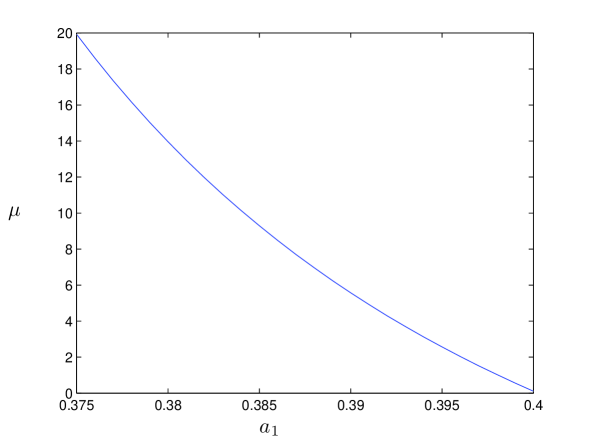
Figure 4: The constant $\mu>0$ of Eq. (36), plotted against the permitted range of parameter values of $a_{1}$, given by Eq. (35).

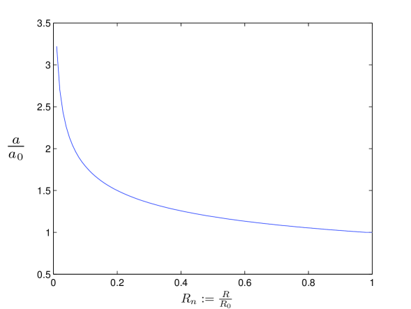
Figure 5: The scale factor as a function of the normalized scalar curvature for the numerically determined cosmological model of Eq. (38).

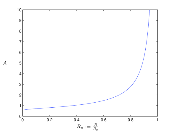
Figure 6: The function $A$, of Eq. (31) as a function of the normalized scalar curvature for the numerically determined cosmological model of Eq. (38).

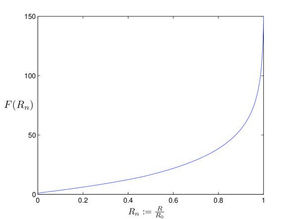
Figure 7: The function $F(R_{n})$, of Eq. (5) as a function of the normalized scalar curvature for the numerically determined cosmological model of Eq. (38).

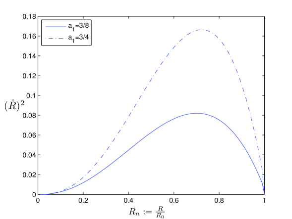
Figure 8: The function of Eq. (18), plotted against the normalized scalar curvature, for permitted range of parameter values of $a_{1}$, given by Eq. (35).

References

- [1] S. Capozziello, M. De Laurentis and V. Faraoni, Invited review for the special issue in Cosmology, The open Astronomy Journal, Eds. S. D. Odintsov et al., [arXiv:0909.4672v2 [gr-qc]]
- [2] S. Capozziello and M. Frangaviglia, Gen. Rel. Grav. 40 (2008) 357-420, [arXiv:0706.1146 [astro-ph]]
- [3] T. P. Sotiriou and V. Faraoni, Rev. Mod. Phys. 82 (2010) 451-497, [arXiv:0805.1726 [gr-qc]]
- [4] V. Faraoni, Presented at SIGRAV2008, 18th Congress of the Italian Society of General Relativity and Gravitation, Cosenza, Italy September 22-25, 2008, [arXiv:0810.2602 [gr-qc]]
- [5] H. Shabani and A. H. Ziaie, [arXiv:1708.07874v1 [gr-qc]]
- [6] W. H. Kinney, Lectures from the 2008 Theoretical Advanced Study Institiute at Univ. of Colorado, Boulder, [arXiv:0902.1529v2 [astro-ph.CO]]
- [7] S. W. Hawking and R. Penrose, Proc. Royal. Soc. London A 314 (1970) 529; S. W. Hawking and G. F. R. Ellis, The Large Scale Structure of Space-Time, Cambridge University Press (1975)
- [8] K. Bamba, A. N. Makarenko, A. N. Myayky, S. Nojiri and S. D. Odintsov, JCAP 01 (2014) 008 [arXiv:1309.3748v2 [hep-th]]
- [9] T. Clifton, Phys. Rev. D 78 (2008) 083501, [arXiv:0807.4682 [gr-qc]]
- [10] N. Goheer, R. Goswami and P. K. S. Dunsby, Class. Quant. Grav. 26 (2009) 105003, [arXiv:0809.5247 [gr-qc]]
- [11] C. Barragan, G. J. Olmc and H. Sanchis-Alepuz, Phys. Rev. D 80 (2009) 024016, [arXiv: 0907.0318 [gr-qc]]
- [12] T. S. Koivisto, Phys. Rev. D 82 (2010) 044022, [arXiv:1004.4298 [gr-qc]]
- [13] H. Farajollahi, M. Setare, F. Milani and F. Tayebi, Gen. Rel. Grav. 43 (2011) 1657, [arXiv:1005.2026 [phys.gen-ph]]
- [14] C. Barragan and G. J. Olmo, Phys. Rev. D 82 (2010) 084015, [arXiv:1005.4136 [gr-qc]]
- [15] Yi-Fu Cai and E. N. Saridakis, Class. Quant. Grav. 28 (2011) 035010, [arXiv:1007.3204 [astro-ph.CO]]
- [16] G. J. Olmo, Int. J. Mod. Phys. D 20 (2011) 413, [arXiv:1101.3864 [gr-qc]]
- [17] G. J. Olmo, J. Phys. Conf. Ser. 314 (2011) 012054, [arXiv:1101.4913 [gr-qc]]
- [18] T. Harko, F. S. N. Lobo, S. Nojiri and S. D. Odintsov, Phys. Rev. D 84 (2011) 024020, [arXiv:1104.2669 [gr-qc]]
- [19] S. K. Chakrabarti, K. Dutta and A. A. Sen, Phys. Lett. B 711 (2012) 147, [arXiv:1108.2781 [astro-ph.CO]]
- [20] J. C. Fubris, R. S. Perez, S. E. Perez-Bergliaffa and N. Pinto-Neto, Phys. Rev. D 86 (2012) 103525, [arXiv:1205.3458 [gr-qc]]
- [21] I. Dimitrijevic, B. Dragovich, J. Grujic and Z. Rakic, Rom. Journ. Phys. 58 (5-6) (2013) 550, [arXiv:1302.2794 [gr-qc]]
- [22] S. Nojiri and S. D. Odintsov, Problems of Modern Theoretical Physics, a volume in honour of Prof. I. L. Buchbinder in occasion of his 60th birthday, p. 266-285 TSPU Publishing Tomsk, [arXiv:0807.0685 [hep-th]]
- [23] S. Capozziello, E. Elizalde, S. Nojiri and S. D. Odintsov, Phys. Lett. B 671 (2009) 193-198, [arXiv:0809.1535v2 [hep-th]]
- [24] S. Bahamonde, S. D. Odintsov, V. K. Oikonomou and P. V. Tretyakov, Phys. Lett. B 766 (2017) 225-230, [arXiv:1701.02381v2 [gr-qc]]
- [25] T. Harko, T. S. Koivisto, F. S. N. Lobo and G. J. Olmo, Phys. Rev. D 85 (2012) 084016, [arXiv:1110.1049[gr-qc]]
- [26] H. Farajollahi, F. Tayebi, F. Milani and M. Enayati, Astr. Sp. Science 337, 2 (2012) 773-778, [arXiv:1110.3668 [gr-qc]]
- [27] R. Myrzakulov and L. Sebastiani, Astrophys.Space Sci. 352 (2014) 281-288, [arXiv:1403.0681 [gr-qc]]
- [28] M. Ghanaatian and F. Milani, Gen. Rel. Grav. 46 (2014) 1789, [arXiv:1403.6178 [physics.gen-ph]]
- [29] A. N. Makarenko, S. D. Odintsov and G. J. Olmo, Phys. Rev. D 90 (2014) 024066, [arXiv:1403.7409 [hep-th]]
- [30] P. Niladri, S. N. Chakrabarty and K. Bhattacharya, JCAP 1410 (2014) 10, 009, [arXiv:1405.0139 [gr-qc]]
- [31] S.D. Odintsov and V.K. Oikonomou, Phys. Rev. D 90 (2014) 124083, [arXiv:1410.8183 [gr-qc]]
- [32] V.K. Oikonomou, Astrophys. Space Sci. (2015) 359: 30, [arXiv:1412.4343 [gr-qc]]
- [33] S.D. Odintsov, V.K. Oikonomou and E. N. Saridakis, Annals Phys. 363 (2015) 141-163, [arXiv:1501.06591 [gr-qc]]
- [34] D. Momeni, R. Myrzakulov and E. Gudekli, Int. J. Geom. Methods Mod. Phys. 12 (2015) 1550101, [arXiv:1502.00977 [gr-qc]]
- [35] S.D. Odintsov and V.K. Oikonomou, Phys. Rev. D 91 (2015) 064036, [arXiv:1502.06125 [gr-qc]]
- [36] S.D. Odintsov and V.K. Oikonomou, Phys. Rev. D 92 (2015) 024016, [arXiv:1504.06866 [gr-qc]]
- [37] K. Bhattacharya and S. Chakrabarty, JCAP 02 (2016) 030, [arXiv:1509.01835 [gr-qc]]
- [38] S.D. Odintsov and V.K. Oikonomou, Phys. Rev. D 93 (2016) 023517, [arXiv:1511.04559 [gr-qc]]
- [39] A. R. Amani, Int. J. Mod. Phys. D 25 (2016) 1650071, [arXiv:1512.03475 [gr-qc]]
- [40] S.D. Odintsov and V.K. Oikonomou, Int. J. Mod. Phys. D 26 (2017) 1750085, [arXiv:1512.04787 [gr-qc]]
- [41] S. Nojiri, S.D. Odintsov and V.K. Oikonomou, Phys. Rev. D 93 (2016) 084050, [arXiv:1601.04112 [gr-qc]]
- [42] T. Miranda, J. C. Fabris and O. F. Piattella, JCAP 1709 (2017) no.09, 041, [arXiv:1707.06457 [gr-qc]]
- [43] S. Nojiri, S.D. Odintsov and V.K. Oikonomou, Phys.Rept. 692 (2017) 1-104, [arXiv:1705.11098 [gr-qc]]