Supplementary Materials for
Uncertainty conservation relations: theory and experiment

Hengyan Wang These authors contributed equally to this work. CAS Key Laboratory of Microscale Magnetic Resonance and Department of Modern Physics, University of Science and Technology of China, Hefei 230026, China    Zhihao Ma These authors contributed equally to this work. Department of Mathematics, Shanghai Jiaotong University, Shanghai 200240, China    Shengjun Wu These authors contributed equally to this work. Kuang Yaming Honors School, Nanjing University, Nanjing, Jiangsu 210023, China    Wenqiang Zheng Department of Applied Physics, Zhejiang University of Technology, Hangzhou, Zhejiang 310023, China    Zhu Cao Center for Quantum Information, Institute for Interdisciplinary Information Sciences, Tsinghua University, Beijing 100084 China    Zhihua Chen Department of Applied Physics, Zhejiang University of Technology, Hangzhou, Zhejiang 310023, China    Zhaokai Li CAS Key Laboratory of Microscale Magnetic Resonance and Department of Modern Physics, University of Science and Technology of China, Hefei 230026, China Synergetic Innovation Center of Quantum Information and Quantum Physics, University of Science and Technology of China, Hefei 230026, China    Shao-Ming Fei School of Mathematical Sciences, Capital Normal University, Beijing 100048, China Max-Planck-Institute for Mathematics in the Sciences, 04103 Leipzig, Germany    Xinhua Peng xhpeng@ustc.edu.cn CAS Key Laboratory of Microscale Magnetic Resonance and Department of Modern Physics, University of Science and Technology of China, Hefei 230026, China Synergetic Innovation Center of Quantum Information and Quantum Physics, University of Science and Technology of China, Hefei 230026, China    Vlatko Vedral phyvv@nus.edu.sg Atomic and Laser Physics, University of Oxford, Clarendon Laboratory, Parks Road, Oxford, OX1 3PU, United Kingdom Centre for Quantum Technologies, National University of Singapore, 3 Science Drive 2, 117543 Singapore    Jiangfeng Du djf@ustc.edu.cn CAS Key Laboratory of Microscale Magnetic Resonance and Department of Modern Physics, University of Science and Technology of China, Hefei 230026, China Synergetic Innovation Center of Quantum Information and Quantum Physics, University of Science and Technology of China, Hefei 230026, China

I Proof of the theorem

I.1 Mutually unbiased bases and bipartite basis states

In a d𝑑d-dimensional Hilbert space \mathcal{H}, let {|iθ|i=1,,d}conditionalketsubscript𝑖𝜃𝑖1𝑑\{\left|i_{\theta}\right\rangle|i=1,\cdots,d\} denote a basis labeled by θ𝜃\theta. A set of M𝑀M such bases is called mutually unbiased if

|iθ|jτ|2=1dsuperscriptinner-productsubscript𝑖𝜃subscript𝑗𝜏21𝑑|\left\langle i_{\theta}|j_{\tau}\right\rangle|^{2}=\frac{1}{d} (1)

for any i,j=1,2,,dformulae-sequence𝑖𝑗12𝑑i,j=1,2,\cdots,d, and θ,τ=1,,Mformulae-sequence𝜃𝜏1𝑀\theta,\tau=1,\cdots,M with θτ𝜃𝜏\theta\neq\tau. When d𝑑d is a power of a prime number, a complete set of d+1𝑑1d+1 MUBs exists. When d𝑑d is an arbitrary integer number, the maximal number of MUBs is unknown. For example, when d=6𝑑6d=6, only 333 MUBs have yet been found. However, for any d2𝑑2d\geqslant 2, there exist at least 333 MUBs. For the purpose of this paper, we only assume that M𝑀M MUBs are available in a d𝑑d-dimensional Hilbert space, where M𝑀M is less than or equal to the maximal number of MUBs that can exist.

In a composite Hilbert space tensor-product\mathcal{H}\otimes\mathcal{H} of two qudits, we construct the following M(d1)+1𝑀𝑑11M(d-1)+1 states,

|ΦketΦ\displaystyle|\Phi\rangle =\displaystyle= 1di=1d|i1A|i1B,1𝑑superscriptsubscript𝑖1𝑑tensor-productsubscriptketsubscript𝑖1𝐴superscriptsubscriptketsubscript𝑖1𝐵\displaystyle\frac{1}{\sqrt{d}}\sum_{i=1}^{d}|i_{1}\rangle_{A}\otimes|i_{1}\rangle_{B}^{*}, (2)
|ϕθ,kketsubscriptitalic-ϕ𝜃𝑘\displaystyle|\phi_{\theta,k}\rangle =\displaystyle= 1di=1dωk(i1)|iθA|iθB1𝑑superscriptsubscript𝑖1𝑑tensor-productsuperscript𝜔𝑘𝑖1subscriptketsubscript𝑖𝜃𝐴superscriptsubscriptketsubscript𝑖𝜃𝐵\displaystyle\frac{1}{\sqrt{d}}\sum_{i=1}^{d}\omega^{k(i-1)}|i_{\theta}\rangle_{A}\otimes|i_{\theta}\rangle_{B}^{*} (3)

with ω=e2πi/d𝜔superscript𝑒2𝜋𝑖𝑑\omega=e^{2\pi i/d}, k=1,,d1𝑘1𝑑1k=1,\ldots,d-1 and θ=1,2,,M𝜃12𝑀\theta=1,2,\ldots,M. Here |iθsuperscriptketsubscript𝑖𝜃|i_{\theta}\rangle^{*} denotes the complex conjugate of |iθketsubscript𝑖𝜃|i_{\theta}\rangle with respect to the computational basis (which can be chosen as the first basis {|i1}ketsubscript𝑖1\{|i_{1}\rangle\} without loss of generality). It is straightforward to show the following proposition.

Proposition 1. The M(d1)+1𝑀𝑑11M(d-1)+1 bipartite states defined in Eqs. (2, 3) are normalized and orthogonal to each other.

Therefore, these M(d1)+1𝑀𝑑11M(d-1)+1 states can be used for constructing a basis in the composite Hilbert space tensor-product\mathcal{H}\otimes\mathcal{H}. Since there are at most d2superscript𝑑2d^{2} orthogonal states in a d2superscript𝑑2d^{2}-dimensional space, one has M(d1)+1d2𝑀𝑑11superscript𝑑2M(d-1)+1\leqslant d^{2}, which implies Md+1𝑀𝑑1M\leqslant d+1, i.e., there are at most d+1𝑑1d+1 MUBs for a d𝑑d-dimensional Hilbert space. When M=d+1𝑀𝑑1M=d+1, i.e., a complete set of d+1𝑑1d+1 MUBs in a d𝑑d-dimensional space is available, the states defined in Eqs. (2,3) constitute a complete basis for the composite Hilbert space tensor-product\mathcal{H}\otimes\mathcal{H}. On the other hand, when M<d+1𝑀𝑑1M<d+1, one can complete a basis of the composite Hilbert space by adding p=(d1)(d+1M)𝑝𝑑1𝑑1𝑀p=(d-1)(d+1-M) additional orthonormal states {|φα|α=1,,p}conditionalketsubscript𝜑𝛼𝛼1𝑝\{\left|\varphi_{\alpha}\right\rangle|\alpha=1,\cdots,p\}. The projector onto the subspace spanned by these additional states is denoted by 𝒫𝒫\mathcal{P}, i.e.,

𝒫=II|ΦΦ|θ=1Mk=1d1|ϕθ,kϕθ,k|=α=1p|φαφα|.𝒫tensor-product𝐼𝐼ketΦquantum-operator-productΦsuperscriptsubscript𝜃1𝑀superscriptsubscript𝑘1𝑑1subscriptitalic-ϕ𝜃𝑘brasubscriptitalic-ϕ𝜃𝑘superscriptsubscript𝛼1𝑝ketsubscript𝜑𝛼brasubscript𝜑𝛼\mathcal{P}=I\otimes I-\left|\Phi\right\rangle\left\langle\Phi\right|-\sum_{\theta=1}^{M}\sum_{k=1}^{d-1}\left|\phi_{\theta,k}\right\rangle\left\langle\phi_{\theta,k}\right|=\sum_{\alpha=1}^{p}\left|\varphi_{\alpha}\right\rangle\left\langle\varphi_{\alpha}\right|. (4)

It is obvious that 𝒫=0𝒫0\mathcal{P}=0 when M=d+1𝑀𝑑1M=d+1.

Let T2subscript𝑇2T_{2} denote the partial transpose with respect to the computational basis of the second Hilbert space. One immediately has

(|ΦΦ|)T2=1di,j=1d|i1j1||j1i1|.superscriptketΦbraΦsubscript𝑇21𝑑superscriptsubscript𝑖𝑗1𝑑tensor-productketsubscript𝑖1brasubscript𝑗1ketsubscript𝑗1brasubscript𝑖1(\left|\Phi\right\rangle\left\langle\Phi\right|)^{T_{2}}=\frac{1}{d}\sum_{i,j=1}^{d}\left|i_{1}\right\rangle\left\langle j_{1}\right|\otimes\left|j_{1}\right\rangle\left\langle i_{1}\right|.\\ (5)

As k=1d1ωk(ij)superscriptsubscript𝑘1𝑑1superscript𝜔𝑘𝑖𝑗\sum_{k=1}^{d-1}\omega^{k(i-j)} equals to 11-1 for ij𝑖𝑗i\neq j and d1𝑑1d-1 when i=j𝑖𝑗i=j, it is not difficult to show

(k=1d1|ϕθ,kϕθ,k|)T2superscriptsuperscriptsubscript𝑘1𝑑1ketsubscriptitalic-ϕ𝜃𝑘brasubscriptitalic-ϕ𝜃𝑘subscript𝑇2\displaystyle\left(\sum_{k=1}^{d-1}\left|\phi_{\theta,k}\right\rangle\left\langle\phi_{\theta,k}\right|\right)^{T_{2}} =\displaystyle= i=1d|iθiθ||iθiθ|superscriptsubscript𝑖1𝑑tensor-productketsubscript𝑖𝜃brasubscript𝑖𝜃ketsubscript𝑖𝜃brasubscript𝑖𝜃\displaystyle\sum_{i=1}^{d}\left|i_{\theta}\right\rangle\left\langle i_{\theta}\right|\otimes\left|i_{\theta}\right\rangle\left\langle i_{\theta}\right| (6)
\displaystyle- 1di,j=1d|iθjθ||jθiθ|.1𝑑superscriptsubscript𝑖𝑗1𝑑tensor-productketsubscript𝑖𝜃brasubscript𝑗𝜃ketsubscript𝑗𝜃brasubscript𝑖𝜃\displaystyle\frac{1}{d}\sum_{i,j=1}^{d}\left|i_{\theta}\right\rangle\left\langle j_{\theta}\right|\otimes\left|j_{\theta}\right\rangle\left\langle i_{\theta}\right|.

I.2 A useful nonnegative-definite operator

Suppose ρABsubscript𝜌𝐴𝐵\rho_{AB} is a bipartite state on the composite Hilbert space ABtensor-productsubscript𝐴subscript𝐵\mathcal{H}_{A}\otimes\mathcal{H}_{B} of dimension d×D𝑑𝐷d\times D, and suppose {|iθA}subscriptketsubscript𝑖𝜃𝐴\{\left|i_{\theta}\right\rangle_{A}\} is the θ𝜃\theta-th MUB in the d𝑑d-dimensional Hilbert space Asubscript𝐴\mathcal{H}_{A}, after system A𝐴A is projected onto the θ𝜃\theta-th MUB the overall bipartite state is written as

ρθB=i=1d|iθAiθ|Aiθ|ρAB|iθA.subscript𝜌𝜃𝐵superscriptsubscript𝑖1𝑑subscripttensor-product𝐴subscriptketsubscript𝑖𝜃𝐴brasubscript𝑖𝜃subscriptquantum-operator-productsubscript𝑖𝜃subscript𝜌𝐴𝐵subscript𝑖𝜃𝐴\rho_{\theta B}=\sum_{i=1}^{d}\left|i_{\theta}\right\rangle_{A}\left\langle i_{\theta}\right|\otimes_{A}\left\langle i_{\theta}\right|\rho_{AB}\left|i_{\theta}\right\rangle_{A}. (7)

Given a bipartite state ρABsubscript𝜌𝐴𝐵\rho_{AB} and a set of M𝑀M MUBs in Asubscript𝐴\mathcal{H}_{A}, we define an operator

ΓABIAρB+M1dρABθ=1MρθBsubscriptΓ𝐴𝐵tensor-productsubscript𝐼𝐴subscript𝜌𝐵𝑀1𝑑subscript𝜌𝐴𝐵superscriptsubscript𝜃1𝑀subscript𝜌𝜃𝐵\Gamma_{AB}\equiv I_{A}\otimes\rho_{B}+\frac{M-1}{d}\rho_{AB}-\sum_{\theta=1}^{M}\rho_{\theta B} (8)

on ABtensor-productsubscript𝐴subscript𝐵\mathcal{H}_{A}\otimes\mathcal{H}_{B}. This operator is Hermitian, and it has the following nice property.

Proposition 2. When M=d+1𝑀𝑑1M=d+1, the operator ΓABsubscriptΓ𝐴𝐵\Gamma_{AB} vanishes: ΓAB=0subscriptΓ𝐴𝐵0\Gamma_{AB}=0. When Md𝑀𝑑M\leqslant d, it is nonnegative-definite

ΓAB0.subscriptΓ𝐴𝐵0\Gamma_{AB}\geqslant 0. (9)

In order to prove proposition 2, we introduce an additional Hilbert space Csubscript𝐶\mathcal{H}_{C} of dimension d𝑑d, and introduce a linear map \mathcal{F} that maps operators on Csubscript𝐶\mathcal{H}_{C} to operators on Asubscript𝐴\mathcal{H}_{A}, such that (|i1Cj1|)=|i1Aj1|subscriptketsubscript𝑖1𝐶brasubscript𝑗1subscriptketsubscript𝑖1𝐴brasubscript𝑗1\mathcal{F}(\left|i_{1}\right\rangle_{C}\left\langle j_{1}\right|)=\left|i_{1}\right\rangle_{A}\left\langle j_{1}\right| (i,j=1,,dformulae-sequence𝑖𝑗1𝑑i,j=1,\cdots,d). One can easily show that (|iθCjθ|)=|iθAjθ|subscriptketsubscript𝑖𝜃𝐶brasubscript𝑗𝜃subscriptketsubscript𝑖𝜃𝐴brasubscript𝑗𝜃\mathcal{F}(\left|i_{\theta}\right\rangle_{C}\left\langle j_{\theta}\right|)=\left|i_{\theta}\right\rangle_{A}\left\langle j_{\theta}\right| for θ=1,,M𝜃1𝑀\theta=1,\cdots,M. Let 1superscript1\mathcal{F}^{-1} denote the inverse map, and let ρCB1(ρAB)subscript𝜌𝐶𝐵superscript1subscript𝜌𝐴𝐵\rho_{CB}\equiv\mathcal{F}^{-1}(\rho_{AB}) denote the corresponding state on CBtensor-productsubscript𝐶subscript𝐵\mathcal{H}_{C}\otimes\mathcal{H}_{B} with respect to the state ρABsubscript𝜌𝐴𝐵\rho_{AB} on ABtensor-productsubscript𝐴subscript𝐵\mathcal{H}_{A}\otimes\mathcal{H}_{B}. Therefore, the map :ρCB(ρCB):subscript𝜌𝐶𝐵subscript𝜌𝐶𝐵\mathcal{F}:\rho_{CB}\rightarrow\mathcal{F}(\rho_{CB}) can also be conveniently written via a partial trace over system C𝐶C

(ρCB)subscript𝜌𝐶𝐵\displaystyle\mathcal{F}(\rho_{CB}) =\displaystyle= ijTrC{[|iθAjθ||jθCiθ|]ρCB}subscript𝑖𝑗𝑇subscript𝑟𝐶delimited-[]tensor-productsubscriptketsubscript𝑖𝜃𝐴brasubscript𝑗𝜃subscriptketsubscript𝑗𝜃𝐶brasubscript𝑖𝜃subscript𝜌𝐶𝐵\displaystyle\sum_{ij}Tr_{C}\left\{\left[\left|i_{\theta}\right\rangle_{A}\left\langle j_{\theta}\right|\otimes\left|j_{\theta}\right\rangle_{C}\left\langle i_{\theta}\right|\right]\rho_{CB}\right\}
=\displaystyle= ij|iθAjθ|iθ|ρCB|jθsubscript𝑖𝑗tensor-productsubscriptketsubscript𝑖𝜃𝐴brasubscript𝑗𝜃quantum-operator-productsubscript𝑖𝜃subscript𝜌𝐶𝐵subscript𝑗𝜃\displaystyle\sum_{ij}\left|i_{\theta}\right\rangle_{A}\left\langle j_{\theta}\right|\otimes\left\langle i_{\theta}\right|\rho_{CB}\left|j_{\theta}\right\rangle
=\displaystyle= ρABsubscript𝜌𝐴𝐵\displaystyle\rho_{AB}

for any θ{1,,M}𝜃1𝑀\theta\in\{1,\cdots,M\}. Similarly, ρθBsubscript𝜌𝜃𝐵\rho_{\theta B} can be written as

ρθB=TrC{[i=1d|iθAiθ||iθCiθ|]ρCB}.subscript𝜌𝜃𝐵𝑇subscript𝑟𝐶delimited-[]superscriptsubscript𝑖1𝑑tensor-productsubscriptketsubscript𝑖𝜃𝐴brasubscript𝑖𝜃subscriptketsubscript𝑖𝜃𝐶brasubscript𝑖𝜃subscript𝜌𝐶𝐵\rho_{\theta B}=Tr_{C}\left\{\left[\sum_{i=1}^{d}\left|i_{\theta}\right\rangle_{A}\left\langle i_{\theta}\right|\otimes\left|i_{\theta}\right\rangle_{C}\left\langle i_{\theta}\right|\right]\rho_{CB}\right\}. (11)

Hence

θ=1M(1dρABρθB)superscriptsubscript𝜃1𝑀1𝑑subscript𝜌𝐴𝐵subscript𝜌𝜃𝐵\displaystyle\sum_{\theta=1}^{M}(\frac{1}{d}\rho_{AB}-\rho_{\theta B}) (12)
=\displaystyle= θ=1MTrC{1dij|iθAjθ||jθCiθ|ρCB}superscriptsubscript𝜃1𝑀𝑇subscript𝑟𝐶1𝑑subscript𝑖𝑗tensor-productsubscriptketsubscript𝑖𝜃𝐴brasubscript𝑗𝜃subscriptketsubscript𝑗𝜃𝐶brasubscript𝑖𝜃subscript𝜌𝐶𝐵\displaystyle\sum_{\theta=1}^{M}Tr_{C}\left\{\frac{1}{d}\sum_{ij}\left|i_{\theta}\right\rangle_{A}\left\langle j_{\theta}\right|\otimes\left|j_{\theta}\right\rangle_{C}\left\langle i_{\theta}\right|\rho_{CB}\right\}
θ=1MTrC{i|iθAiθ||iθCiθ|ρCB}superscriptsubscript𝜃1𝑀𝑇subscript𝑟𝐶subscript𝑖tensor-productsubscriptketsubscript𝑖𝜃𝐴brasubscript𝑖𝜃subscriptketsubscript𝑖𝜃𝐶brasubscript𝑖𝜃subscript𝜌𝐶𝐵\displaystyle-\sum_{\theta=1}^{M}Tr_{C}\left\{\sum_{i}\left|i_{\theta}\right\rangle_{A}\left\langle i_{\theta}\right|\otimes\left|i_{\theta}\right\rangle_{C}\left\langle i_{\theta}\right|\rho_{CB}\right\}
=\displaystyle= TrC{(θ=1Mk=1d1|ϕθ,kACϕθ,k|)TCρCB}.𝑇subscript𝑟𝐶superscriptsuperscriptsubscript𝜃1𝑀superscriptsubscript𝑘1𝑑1subscriptketsubscriptitalic-ϕ𝜃𝑘𝐴𝐶brasubscriptitalic-ϕ𝜃𝑘subscript𝑇𝐶subscript𝜌𝐶𝐵\displaystyle-Tr_{C}\left\{\left(\sum_{\theta=1}^{M}\sum_{k=1}^{d-1}\left|\phi_{\theta,k}\right\rangle_{AC}\left\langle\phi_{\theta,k}\right|\right)^{T_{C}}\rho_{CB}\right\}.

We have used Eq. (6) to obtain the last equality. From Eqs. (5) and (I.2) with θ=1𝜃1\theta=1, we also have

1dρAB=TrC{(|ΦACΦ|)TCρCB}.1𝑑subscript𝜌𝐴𝐵𝑇subscript𝑟𝐶superscriptsubscriptketΦ𝐴𝐶braΦsubscript𝑇𝐶subscript𝜌𝐶𝐵\frac{1}{d}\rho_{AB}=Tr_{C}\left\{(\left|\Phi\right\rangle_{AC}\left\langle\Phi\right|)^{T_{C}}\rho_{CB}\right\}. (13)

From Eqs. (12) and (13) and the obvious relation IAρB=TrC[(IaIC)ρCB]tensor-productsubscript𝐼𝐴subscript𝜌𝐵𝑇subscript𝑟𝐶delimited-[]tensor-productsubscript𝐼𝑎subscript𝐼𝐶subscript𝜌𝐶𝐵I_{A}\otimes\rho_{B}=Tr_{C}[(I_{a}\otimes I_{C})\rho_{CB}], we can rewrite ΓABsubscriptΓ𝐴𝐵\Gamma_{AB} as

ΓABsubscriptΓ𝐴𝐵\displaystyle\Gamma_{AB} =\displaystyle= IAρB1dρAB+θ=1M(1dρABρθB)tensor-productsubscript𝐼𝐴subscript𝜌𝐵1𝑑subscript𝜌𝐴𝐵superscriptsubscript𝜃1𝑀1𝑑subscript𝜌𝐴𝐵subscript𝜌𝜃𝐵\displaystyle I_{A}\otimes\rho_{B}-\frac{1}{d}\rho_{AB}+\sum_{\theta=1}^{M}(\frac{1}{d}\rho_{AB}-\rho_{\theta B}) (14)
=\displaystyle= TrC{𝒫ACTCρCB}.𝑇subscript𝑟𝐶superscriptsubscript𝒫𝐴𝐶subscript𝑇𝐶subscript𝜌𝐶𝐵\displaystyle Tr_{C}\left\{\mathcal{P}_{AC}^{T_{C}}\rho_{CB}\right\}.

Here the operator 𝒫ACsubscript𝒫𝐴𝐶\mathcal{P}_{AC} is the projector defined on ACtensor-productsubscript𝐴subscript𝐶\mathcal{H}_{A}\otimes\mathcal{H}_{C} according to (4), i.e.,

𝒫ACsubscript𝒫𝐴𝐶\displaystyle\mathcal{P}_{AC} =\displaystyle= II|ΦΦ|θ=1Mk=1d1|ϕθ,kϕθ,k|tensor-product𝐼𝐼ketΦquantum-operator-productΦsuperscriptsubscript𝜃1𝑀superscriptsubscript𝑘1𝑑1subscriptitalic-ϕ𝜃𝑘brasubscriptitalic-ϕ𝜃𝑘\displaystyle I\otimes I-\left|\Phi\right\rangle\left\langle\Phi\right|-\sum_{\theta=1}^{M}\sum_{k=1}^{d-1}\left|\phi_{\theta,k}\right\rangle\left\langle\phi_{\theta,k}\right| (15)
=\displaystyle= α=1p|φαACφα|.superscriptsubscript𝛼1𝑝subscriptketsubscript𝜑𝛼𝐴𝐶brasubscript𝜑𝛼\displaystyle\sum_{\alpha=1}^{p}\left|\varphi_{\alpha}\right\rangle_{AC}\left\langle\varphi_{\alpha}\right|.

When M=d+1𝑀𝑑1M=d+1, then p=0𝑝0p=0, the states |φαACsubscriptketsubscript𝜑𝛼𝐴𝐶\left|\varphi_{\alpha}\right\rangle_{AC} in ACtensor-productsubscript𝐴subscript𝐶\mathcal{H}_{A}\otimes\mathcal{H}_{C} do not exist, both 𝒫ACsubscript𝒫𝐴𝐶\mathcal{P}_{AC} and ΓABsubscriptΓ𝐴𝐵\Gamma_{AB} vanish. When Md𝑀𝑑M\leqslant d, we have

ΓABsubscriptΓ𝐴𝐵\displaystyle\Gamma_{AB} =\displaystyle= TrC{α=1p(|φαACφα|)TCρCB}𝑇subscript𝑟𝐶superscriptsubscript𝛼1𝑝superscriptsubscriptketsubscript𝜑𝛼𝐴𝐶brasubscript𝜑𝛼subscript𝑇𝐶subscript𝜌𝐶𝐵\displaystyle Tr_{C}\left\{\sum_{\alpha=1}^{p}\left(\left|\varphi_{\alpha}\right\rangle_{AC}\left\langle\varphi_{\alpha}\right|\right)^{T_{C}}\rho_{CB}\right\}
=\displaystyle= α=1pTrC{(|φαACφα|)TCρCB}superscriptsubscript𝛼1𝑝𝑇subscript𝑟𝐶superscriptsubscriptketsubscript𝜑𝛼𝐴𝐶brasubscript𝜑𝛼subscript𝑇𝐶subscript𝜌𝐶𝐵\displaystyle\sum_{\alpha=1}^{p}Tr_{C}\left\{\left(\left|\varphi_{\alpha}\right\rangle_{AC}\left\langle\varphi_{\alpha}\right|\right)^{T_{C}}\rho_{CB}\right\}
=\displaystyle= α=1pTrC{(|φαAC)TCρCB(φα|AC)TC}.superscriptsubscript𝛼1𝑝𝑇subscript𝑟𝐶superscriptsubscriptketsubscript𝜑𝛼𝐴𝐶subscript𝑇𝐶subscript𝜌𝐶𝐵superscriptsubscriptbrasubscript𝜑𝛼𝐴𝐶subscript𝑇𝐶\displaystyle\sum_{\alpha=1}^{p}Tr_{C}\left\{\left(\left|\varphi_{\alpha}\right\rangle_{AC}\right)^{T_{C}}\rho_{CB}\left(\left\langle\varphi_{\alpha}\right|_{AC}\right)^{T_{C}}\right\}.

The last equality is due to the fact that operators on Csubscript𝐶\mathcal{H}_{C} can have cyclic permutations under the partial trace over C𝐶C. Let Θα(|φαAC)TCρCBsubscriptΘ𝛼superscriptsubscriptketsubscript𝜑𝛼𝐴𝐶subscript𝑇𝐶subscript𝜌𝐶𝐵\Theta_{\alpha}\equiv\left(\left|\varphi_{\alpha}\right\rangle_{AC}\right)^{T_{C}}\sqrt{\rho_{CB}}, which are operators on ACBtensor-productsubscript𝐴subscript𝐶subscript𝐵\mathcal{H}_{A}\otimes\mathcal{H}_{C}\otimes\mathcal{H}_{B}. Then we have

ΓAB=α=1pTrC{Θα(Θα)}.subscriptΓ𝐴𝐵superscriptsubscript𝛼1𝑝𝑇subscript𝑟𝐶subscriptΘ𝛼superscriptsubscriptΘ𝛼\Gamma_{AB}=\sum_{\alpha=1}^{p}Tr_{C}\left\{\Theta_{\alpha}(\Theta_{\alpha})^{\dagger}\right\}. (16)

Since Θα(Θα)subscriptΘ𝛼superscriptsubscriptΘ𝛼\Theta_{\alpha}(\Theta_{\alpha})^{\dagger} are always nonnegative-definite operators on ACBtensor-productsubscript𝐴subscript𝐶subscript𝐵\mathcal{H}_{A}\otimes\mathcal{H}_{C}\otimes\mathcal{H}_{B}, the operators TrC{Θα(Θα)}𝑇subscript𝑟𝐶subscriptΘ𝛼superscriptsubscriptΘ𝛼Tr_{C}\left\{\Theta_{\alpha}(\Theta_{\alpha})^{\dagger}\right\} are nonnegative-definite operators on ABtensor-productsubscript𝐴subscript𝐵\mathcal{H}_{A}\otimes\mathcal{H}_{B}, so is their sum. Therefore ΓAB0subscriptΓ𝐴𝐵0\Gamma_{AB}\geqslant 0. This completes the proof of proposition 2.

I.3 Uncertainty equality and inequality

According to proposition 2, ΓABsubscriptΓ𝐴𝐵\Gamma_{AB} is a nonnegative-definite operator when Md𝑀𝑑M\leqslant d, and it vanishes when M=d+1𝑀𝑑1M=d+1. Hence, for any nonnegative-definite operator ΠABsubscriptΠ𝐴𝐵\Pi_{AB} on ABtensor-productsubscript𝐴subscript𝐵\mathcal{H}_{A}\otimes\mathcal{H}_{B},

TrAB(ΓABΠAB)0subscriptTr𝐴𝐵subscriptΓ𝐴𝐵subscriptΠ𝐴𝐵0{\rm Tr}_{AB}(\Gamma_{AB}\Pi_{AB})\geqslant 0 (17)

when Md𝑀𝑑M\leqslant d, and the inequality becomes an equality when M=d+1𝑀𝑑1M=d+1.

Let ΠAB=ρABsubscriptΠ𝐴𝐵subscript𝜌𝐴𝐵\Pi_{AB}=\rho_{AB}, Eq. (17) yields

00\displaystyle 0 \displaystyle\leqslant TrAB(ΓABρAB)subscriptTr𝐴𝐵subscriptΓ𝐴𝐵subscript𝜌𝐴𝐵\displaystyle{\rm Tr}_{AB}(\Gamma_{AB}\rho_{AB}) (18)
=\displaystyle= Tr(ρB2)+M1dTr(ρAB2)θ=1MTr(ρθB2).Trsuperscriptsubscript𝜌𝐵2𝑀1𝑑Trsuperscriptsubscript𝜌𝐴𝐵2superscriptsubscript𝜃1𝑀Trsuperscriptsubscript𝜌𝜃𝐵2\displaystyle{\rm Tr}(\rho_{B}^{2})+\frac{M-1}{d}{\rm Tr}(\rho_{AB}^{2})-\sum_{\theta=1}^{M}{\rm Tr}(\rho_{\theta B}^{2}).

Therefore,

θ=1MTr(ρθB2)Tr(ρB2)M1dTr(ρAB2).superscriptsubscript𝜃1𝑀Trsuperscriptsubscript𝜌𝜃𝐵2Trsuperscriptsubscript𝜌𝐵2𝑀1𝑑Trsuperscriptsubscript𝜌𝐴𝐵2-\sum_{\theta=1}^{M}{\rm Tr}(\rho_{\theta B}^{2})\geqslant-{\rm Tr}(\rho_{B}^{2})-\frac{M-1}{d}{\rm Tr}(\rho_{AB}^{2}). (19)

Adding MTr(ρB2)𝑀Trsuperscriptsubscript𝜌𝐵2M{\rm Tr}(\rho_{B}^{2}) to the above inequality, we immediately have

θ=1M(Tr(ρB2)Tr(ρθB2))(M1)(Tr(ρB2)1dTr(ρAB2)).superscriptsubscript𝜃1𝑀Trsuperscriptsubscript𝜌𝐵2Trsuperscriptsubscript𝜌𝜃𝐵2𝑀1Trsuperscriptsubscript𝜌𝐵21𝑑Trsuperscriptsubscript𝜌𝐴𝐵2\sum_{\theta=1}^{M}({\rm Tr}(\rho_{B}^{2})-{\rm Tr}(\rho_{\theta B}^{2}))\geqslant(M-1)\left({\rm Tr}(\rho_{B}^{2})-\frac{1}{d}{\rm Tr}(\rho_{AB}^{2})\right). (20)

The inequality becomes an equality when M=d+1𝑀𝑑1M=d+1. Thus, the theorem in the main text has been proved.

Remark The approach we admitted here is methodologically similar to the one used in [Phys. Rev. Lett. 83, 3354 (1999)] (see also [Phys. Rev. A. 63, 022113(2001)]). In pra14 an elegant uncertainty equality has also been presented based on ONE positive operator-valued measure consisting uniformly all the measurement operators of d+1𝑑1d+1 MUBs. As we take into account all the d+1𝑑1d+1 MUB projection measurements individually, our uncertainty relation is completely different from the one given in pra14 . In fact, the uncertainty relation in pra14 cannot be applied to our QRNG self-testing scenario, because the equality derived in pra14 holds only when the system is measured in one of the MUBs with uniformly random probability. While our equality holds no matter whether the MUB is uniformly chosen. Such a property is crucial in practical QRNG application, as one needs to restrict the input randomness to choose a mutually unbiased basis.
II Quantum register

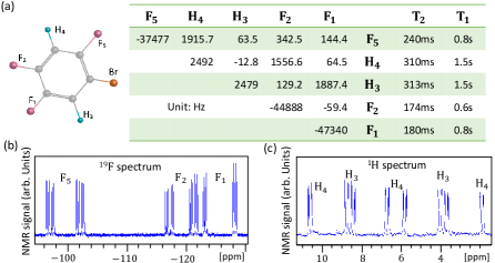
We used the sample named 1-bromo-2,4,5-trifluorobenzene as a 5-qubit NMR quantum system which consists of two 1H spins and three 19F spins, dissolved in the liquid crystal N-(4-methoxybenzylidene)-4-butylaniline. The structure of the molecule is shown in Fig. 1. Due to the partial average effect in the liquid crystal solution, the direct dipole-dipole interaction will be scaled down by the order parameter Dong97 . In our sample, the partial average effect makes the direct dipole-dipole couplings of homonuclear spins much smaller than the difference between the chemical shifts of related nuclear spins, all the dipole-dipole Hamiltonians are reduced to the form of σziσzjsuperscriptsubscript𝜎𝑧𝑖superscriptsubscript𝜎𝑧𝑗{\sigma_{z}^{i}}{\sigma_{z}^{j}}. Therefore, the effective Hamiltonian of the 555-qubit system in rotating frame is

HNMR=i=15πνiσzi+1j<k5π2(Jjk+2Djk)σzjσzk,subscript𝐻NMRsuperscriptsubscript𝑖15𝜋subscript𝜈𝑖superscriptsubscript𝜎𝑧𝑖subscript1𝑗𝑘5𝜋2subscript𝐽𝑗𝑘2subscript𝐷𝑗𝑘superscriptsubscript𝜎𝑧𝑗superscriptsubscript𝜎𝑧𝑘{H_{\mathrm{NMR}}}=\sum\limits_{i=1}^{5}{\pi{\nu_{i}}\sigma_{z}^{i}}+\sum\limits_{1\leq j<k\leq 5}{\frac{\pi}{2}\left({{J_{jk}}+2{D_{jk}}}\right)\sigma_{z}^{j}\sigma_{z}^{k}}, (21)

where σzsubscript𝜎𝑧\sigma_{z} is the pauli operator, νisubscript𝜈𝑖\nu_{i} is the chemical shift of spin-i𝑖i and Jjk+2Djksubscript𝐽𝑗𝑘2subscript𝐷𝑗𝑘{{J_{jk}}+2{D_{jk}}} is the effective coupling constant of spin-j𝑗j and spin-k𝑘k. The relevant parameters are shown in Fig. 1.

Refer to caption
Figure 1: (a) Characteristics of the 1-bromo-2,4,5-trifluorobenzene molecule. The chemical shifts and effective coupling constants (in Hz) are on and above the diagonal in the table, respectively. The last two columns show the transversal relaxation times and the longitudinal relaxation times of each nucleus. (b) The thermal equilibrium 19F and 1H spectra.

III Initial state preparation

We first initialized the quantum register into a labeled pseudo-pure state (LPPS) ρLPPS=εσzprobe|0000ABAB0000|+1/32I32subscript𝜌𝐿𝑃𝑃𝑆tensor-product𝜀superscriptsubscript𝜎𝑧𝑝𝑟𝑜𝑏𝑒subscriptket0000𝐴𝐵superscript𝐴superscript𝐵bra0000132subscript𝐼32\rho_{LPPS}=\varepsilon\sigma_{z}^{probe}\otimes{\left|{0000}\right\rangle_{ABA^{\prime}B^{\prime}}}\langle 0000|+1/32{I_{32}} from the equilibrium state where ε𝜀\varepsilon is the polarization about 105superscript10510^{-5}. We just neglected the identity part because unitary and non-unitary operations all have no influence on it. We applied 303030 unitary operators with the form U=eiβij𝒱ij𝑈superscript𝑒𝑖subscript𝛽𝑖𝑗subscript𝒱𝑖𝑗U=e^{-i\beta_{ij}\mathcal{V}_{ij}} to redistribute the populations between energy levels i𝑖i and j𝑗j. Here 𝒱ijsubscript𝒱𝑖𝑗\mathcal{V}_{ij} is the single quantum transition operator between levels i𝑖i and j𝑗j, that is, a 32×32323232\times 32 matrix whose elements are zero except for two elements 𝒱ij(i,j)=𝒱ij(j,i)=1/2subscript𝒱𝑖𝑗𝑖𝑗subscript𝒱𝑖𝑗𝑗𝑖12\mathcal{V}_{ij}(i,j)=\mathcal{V}_{ij}(j,i)=1/2. According to the desired distribution, the angle βijsubscript𝛽𝑖𝑗\beta_{ij} were numerically calculated. In this produce, the unitary operators generated undesired coherence terms that were eliminated by a following field gradient pulse Gz𝐺𝑧Gz. Accordingly, the LPPS ρLPPSsubscript𝜌𝐿𝑃𝑃𝑆\rho_{LPPS} was prepared.

In the following we only consider the deviation part σzprobe|0000ABAB0000|tensor-productsuperscriptsubscript𝜎𝑧𝑝𝑟𝑜𝑏𝑒subscriptket0000𝐴𝐵superscript𝐴superscript𝐵bra0000\sigma_{z}^{probe}\otimes{\left|{0000}\right\rangle_{ABA^{\prime}B^{\prime}}}\langle 0000|. The composite system was prepared into the state

σzprobeρAB(α,x)ρAB(α,x)=σzprobe(x|ψαψα|+1x4I4)(x|ψαψα|+1x4I4),tensor-producttensor-productsuperscriptsubscript𝜎𝑧𝑝𝑟𝑜𝑏𝑒subscript𝜌𝐴𝐵𝛼𝑥subscript𝜌superscript𝐴superscript𝐵𝛼𝑥tensor-productsuperscriptsubscript𝜎𝑧𝑝𝑟𝑜𝑏𝑒𝑥ketsubscript𝜓𝛼brasubscript𝜓𝛼1𝑥4subscript𝐼4𝑥ketsubscript𝜓𝛼brasubscript𝜓𝛼1𝑥4subscript𝐼4\displaystyle\sigma_{z}^{probe}\otimes\rho_{AB}(\alpha,x)\otimes\rho_{A^{\prime}B^{\prime}}(\alpha,x)=\sigma_{z}^{probe}\otimes(x|\psi_{\alpha}\rangle\langle\psi_{\alpha}|+\frac{1-x}{4}I_{4})\otimes(x|\psi_{\alpha}\rangle\langle\psi_{\alpha}|+\frac{1-x}{4}I_{4}), (22)

from σzprobe|00000000|tensor-productsuperscriptsubscript𝜎𝑧𝑝𝑟𝑜𝑏𝑒ket0000bra0000\sigma_{z}^{probe}\otimes|0000\rangle\langle 0000|, where |ψα=cos(α/2)|01sinα/2|10ketsubscript𝜓𝛼𝛼2ket01𝛼2ket10|\psi_{\alpha}\rangle=\cos(\alpha/2)|01\rangle-\sin{\alpha/2}|10\rangle.

Refer to caption
Figure 2: (a) Quantum circuit of preparing σzprobeρAB(α,1)ρAB(α,1)tensor-producttensor-productsuperscriptsubscript𝜎𝑧𝑝𝑟𝑜𝑏𝑒subscript𝜌𝐴𝐵𝛼1subscript𝜌superscript𝐴superscript𝐵𝛼1\sigma_{z}^{probe}\otimes\rho_{AB}(\alpha,1)\otimes\rho_{A^{\prime}B^{\prime}}(\alpha,1) from LPPS. The rectangles represent single-qubit rotations with angles α𝛼\alpha, π/2𝜋2\pi/2 and π𝜋\pi along y𝑦y-axis. Gz𝐺𝑧Gz is the field gradient pulse along z𝑧z-axis. (b) Pulse sequences for preparing σzprobeρAB(π/2,x)ρAB(π/2,x)tensor-producttensor-productsuperscriptsubscript𝜎𝑧𝑝𝑟𝑜𝑏𝑒subscript𝜌𝐴𝐵𝜋2𝑥subscript𝜌superscript𝐴superscript𝐵𝜋2𝑥\sigma_{z}^{probe}\otimes\rho_{AB}(\pi/2,x)\otimes\rho_{A^{\prime}B^{\prime}}(\pi/2,x) with the temporal averaging method. The rotation angles δ1,2,3,4subscript𝛿1234\delta_{1,2,3,4} are arccos[(1x)2]superscript1𝑥2\arccos[(1-x)^{2}], arccos[x(1x)]𝑥1𝑥\arccos[x(1-x)], arccos[x(1x)]𝑥1𝑥\arccos[x(1-x)] and arccos(x2)superscript𝑥2\arccos(x^{2}), which are used to adjust the coefficients of 444 parts in eg. (23).

In the case of x=1𝑥1x=1, the bipartite systems are entangled where the rotation angle α𝛼\alpha varies from 00 to π/2𝜋2\pi/2 for producing different entanglement. α=0𝛼0\alpha=0 corresponds to separable state and α=π/2𝛼𝜋2\alpha=\pi/2 corresponds to the maximally entangled state. Setting α=π/2𝛼𝜋2\alpha=\pi/2 and scanning x𝑥x from 00 to 111 with interval 0.250.250.25, we prepared the states with different mixedness. In preparing σzprobeρAB(π/2,x)ρAB(π/2,x)tensor-producttensor-productsuperscriptsubscript𝜎𝑧𝑝𝑟𝑜𝑏𝑒subscript𝜌𝐴𝐵𝜋2𝑥subscript𝜌superscript𝐴superscript𝐵𝜋2𝑥\sigma_{z}^{probe}\otimes\rho_{AB}(\pi/2,x)\otimes\rho_{A^{\prime}B^{\prime}}(\pi/2,x), we divided it into 444 parts, i.e.,

σzprobe(1x4I2)(1x4I2),tensor-productsuperscriptsubscript𝜎𝑧𝑝𝑟𝑜𝑏𝑒1𝑥4subscript𝐼21𝑥4subscript𝐼2\displaystyle\sigma_{z}^{probe}\otimes(\frac{1-x}{4}I_{2})\otimes(\frac{1-x}{4}I_{2}), (23)
σzprobe(1x4I2)(x|ψπ/2ψπ/2|),tensor-productsuperscriptsubscript𝜎𝑧𝑝𝑟𝑜𝑏𝑒1𝑥4subscript𝐼2𝑥ketsubscript𝜓𝜋2brasubscript𝜓𝜋2\displaystyle\sigma_{z}^{probe}\otimes(\frac{1-x}{4}I_{2})\otimes(x|\psi_{\pi/2}\rangle\langle\psi_{\pi/2}|),
σzprobe(x|ψπ/2ψπ/2|)(1x4I2),tensor-productsuperscriptsubscript𝜎𝑧𝑝𝑟𝑜𝑏𝑒𝑥ketsubscript𝜓𝜋2brasubscript𝜓𝜋21𝑥4subscript𝐼2\displaystyle\sigma_{z}^{probe}\otimes(x|\psi_{\pi/2}\rangle\langle\psi_{\pi/2}|)\otimes(\frac{1-x}{4}I_{2}),
σzprobe(x|ψπ/2ψπ/2|)(x|ψπ/2ψπ/2|),tensor-productsuperscriptsubscript𝜎𝑧𝑝𝑟𝑜𝑏𝑒𝑥ketsubscript𝜓𝜋2brasubscript𝜓𝜋2𝑥ketsubscript𝜓𝜋2brasubscript𝜓𝜋2\displaystyle\sigma_{z}^{probe}\otimes(x|\psi_{\pi/2}\rangle\langle\psi_{\pi/2}|)\otimes(x|\psi_{\pi/2}\rangle\langle\psi_{\pi/2}|),

and adopted the temporal averaging method TemporalAverage to realize them. By summing the four output states, we obtained the desired state σzprobeρAB(π/2,x)ρAB(π/2,x)tensor-producttensor-productsuperscriptsubscript𝜎𝑧𝑝𝑟𝑜𝑏𝑒subscript𝜌𝐴𝐵𝜋2𝑥subscript𝜌superscript𝐴superscript𝐵𝜋2𝑥\sigma_{z}^{probe}\otimes\rho_{AB}(\pi/2,x)\otimes\rho_{A^{\prime}B^{\prime}}(\pi/2,x). The pulse sequences for the state preparation are shown in Fig. 2 b.

IV Experimental procedure

The total experimental procedure is shown in Fig. 3, including the LPPS preparation, the initial state preparation, MUB measurements and the readout of the purities. When the measurement is along y𝑦y-axis, the first and last rotations in the MUB measurement part should be substituted by rotations along x𝑥x and x𝑥-x, and the angles remain also π/2𝜋2\pi/2. In the z𝑧z-axis measurement case, these two rotations are omitted.

Refer to caption
Figure 3: Experimental pulse sequence. The LPPS preparation contains one GRAPE pulse and one z𝑧z-axis gradient pulse. The GRAPE pulse is used to redistribute the populations and the field gradient pulse is used to eliminate the undesired coherences. The operation V(α,x)𝑉𝛼𝑥V(\alpha,x) is to prepare the initial state σzprobeρAB(α,x)ρAB(α,x)tensor-producttensor-productsuperscriptsubscript𝜎𝑧𝑝𝑟𝑜𝑏𝑒subscript𝜌𝐴𝐵𝛼𝑥subscript𝜌superscript𝐴superscript𝐵𝛼𝑥\sigma_{z}^{probe}\otimes\rho_{AB}(\alpha,x)\otimes\rho_{A^{\prime}B^{\prime}}(\alpha,x). Its specific form is shown in Fig. 2. The solid blue rectangle is π/2𝜋2\pi/2 rotation along (y)𝑦(-y)-axis in x𝑥x-measurement and along x𝑥x-axis in y𝑦y-measurement. The dashed blue rectangles denotes π/2𝜋2\pi/2 rotations with the opposite phases to those in solid blue rectangles. No need to operate them in z𝑧z-measurement. The readout part contains two Cswapsubscript𝐶𝑠𝑤𝑎𝑝{C_{swap}} gates applying on subsystems AA𝐴superscript𝐴AA^{\prime} and BB𝐵superscript𝐵BB^{\prime}. The dashed Cswap(AA)subscript𝐶𝑠𝑤𝑎𝑝𝐴superscript𝐴{C_{swap}}(AA^{\prime}) is not required in reading out the purity of subsystem B𝐵B.

V Experimental results of directly measured purities

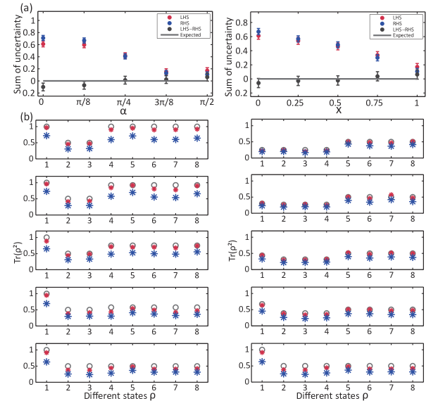
The final experimental signals are influenced by decoherence effect. We simulated the decoherence effect and rescaled the final results. Fig. 4(a) shows the un-rescaled original results. From this we can see that even though the right and left sides of the uncertainty equation are all reduced, they almost equal to each other. Fig. 4(b) shows the directly measured the purities of different states required in the uncertainty conversation relation.

Refer to caption
Figure 4: (a) The original results without rescaling of verifying the uncertainty conservation. The bars are plotted from the infidelity of readout process. (b) The directly measured purities. he hollow dots are the expected purities. The blue asterisks are the directly measured purities and the red ones are the rescaled results. The left five figures correspond to purities when the initial bipartite state is ρAB(α,1)subscript𝜌𝐴𝐵𝛼1\rho_{AB}(\alpha,1) where α=0,π/8,π/4,3π/8,π/2𝛼0𝜋8𝜋43𝜋8𝜋2\alpha=0,\pi/8,\pi/4,3\pi/8,\pi/2 from top to bottom. And the right five figures correspond to ρAB(π/2,x)subscript𝜌𝐴𝐵𝜋2𝑥\rho_{AB}(\pi/2,x) where x=0,0.25,0.5,0.75,1𝑥00.250.50.751x=0,0.25,0.5,0.75,1 from top to bottom. In each figure, from left to right, they are Tr(ρAB2)Trsuperscriptsubscript𝜌𝐴𝐵2{\rm Tr}(\rho_{AB}^{2}), Tr(ρxB2)Trsuperscriptsubscript𝜌𝑥𝐵2{\rm Tr}(\rho_{xB}^{2}), Tr(ρyB2)Trsuperscriptsubscript𝜌𝑦𝐵2{\rm Tr}(\rho_{yB}^{2}), Tr(ρzB2)Trsuperscriptsubscript𝜌𝑧𝐵2{\rm Tr}(\rho_{zB}^{2}), Tr(ρB2)Trsuperscriptsubscript𝜌𝐵2{\rm Tr}(\rho_{B}^{2}), Tr[(ρB|x)2]Trdelimited-[]superscriptsubscript𝜌conditional𝐵𝑥2{\rm Tr}[(\rho_{B|x})^{2}], Tr[(ρB|y)2]Trdelimited-[]superscriptsubscript𝜌conditional𝐵𝑦2{\rm Tr}[(\rho_{B|y})^{2}], Tr[(ρB|z)2]Trdelimited-[]superscriptsubscript𝜌conditional𝐵𝑧2{\rm Tr}[(\rho_{B|z})^{2}], where ρθBsubscript𝜌𝜃𝐵\rho_{\theta B} (θ=x,y,z)𝜃𝑥𝑦𝑧(\theta=x,y,z) are the resulting state after the complete MUB measurements on subsystem A𝐴A, and ρB|θ=TrA(ρθB)subscript𝜌conditional𝐵𝜃subscriptTr𝐴subscript𝜌𝜃𝐵\rho_{B|\theta}={\rm Tr}_{A}(\rho_{\theta B}).

References

  • (1) Dong, R. Y. Nuclear Magnetic Resonance of Liquid Crystals. (Springer, New York, 1997).
  • (2) Knill, E., Chuang, I. & Laflamme, R. Effective pure states for bulk quantum computation. Phys. Rev. A 57, 3348 (1998).
  • (3) Berta, M., Coles, P. J., & Wehner, S. Entanglement-assisted guessing of complementary measurement outcomes. Phys. Rev. A 90, 062127 (2014).