Solar System Science with ESA Euclid

Abstract

Context. The ESA Euclid mission has been designed to map the geometry of the dark Universe. Scheduled for launch in 2020, it will conduct a six-years visible and near-infrared imaging and spectroscopic survey over 15,000 deg² down to V${}_{\textrm{AB}}$$\sim$24.5. Although the survey will avoid ecliptic latitudes below 15°, the survey pattern in repeated sequences of four broad-band filters seems well-adapted to Solar System objects (SSOs) detection and characterization.

Aims. We aim at evaluating Euclid capability to discover SSOs, and measure their position, apparent magnitude, and spectral energy distribution. Also, we investigate how these measurements can lead to the determination of their orbits, morphology (activity and multiplicity), physical properties (rotation period, spin orientation, and 3-D shape), and surface composition.

Methods. We use current census of SSOs to extrapolate the total amount of SSOs detectable by Euclid, i.e., within the survey area and brighter than the limiting magnitude. For each different population of SSO, from neighboring near-Earth asteroids to distant Kuiper-belt objects (KBOs) and including comets, we compare the expected Euclid astrometry, photometry, and spectroscopy with SSO properties to estimate how Euclid will constrain the SSOs dynamical, physical, and compositional properties.

Results. With current survey design, about 150,000 SSOs, mainly from the asteroid main-belt, should be observed by Euclid. These objects will all have high inclination, which contrasts with many SSO surveys focusing on the ecliptic plane. There is a potential for discovery of several 10⁴ SSOs by Euclid, in particular distant KBOs at high declination. Euclid observations, consisting in a suite of four sequences of four measurements, will refine the spectral classification of SSOs by extending the spectral coverage provided by, e.g., Gaia and the LSST to 2 microns. The time-resolved photometry, combined with sparse photometry such as measured by Gaia and the LSST, will contribute to the determination of SSO rotation period, spin orientation, and 3-D shape model. The sharp and stable point-spread function of Euclid will also allow to resolve binary systems in the Kuiper Belt and detect activity around Centaurs.

Conclusions. The depth of Euclid survey (V${}_{\textrm{AB}}$$\sim$24.5), its spectral coverage (0.5 to 2.0 $\mu$m), and observation cadence has great potential for Solar System research. A dedicated processing for SSOs is being set in place within Euclid consortium to produce catalogs of astrometry, multi-color and time-resolved photometry, and spectral classification of some 10⁵ SSOs, delivered as Legacy Science.

1 Introduction

Euclid, the second mission in ESA’s Cosmic Vision program, is a wide-field space mission dedicated to the study of dark energy and dark matter through a mapping of weak gravitational lensing (Laureijs et al., 2011). It is equipped with a silicon-carbide 1.2 m-aperture Korsch telescope and two instruments: a VISible imaging camera and a Near Infrared Spectrometer and Photometer (VIS and NISP, see Cropper et al., 2014; Maciaszek et al., 2014). The mission design combines a large field of view (FoV, 0.57 deg²) with high angular resolution (pixel scales of 0.1″ and 0.3″ for VIS and NISP, corresponding to the diffraction limit at 0.6 and 1.7 $\mu$m).
Scheduled for a launch in 2020 and operating during six years from the Sun-Earth Lagrange L2 point, Euclid will carry out an imaging and spectroscopic survey of the extra-galactic sky of 15,000 deg² (the Wide Survey), avoiding galactic latitudes smaller than 30° and ecliptic latitudes below 15° (Fig. 1), totaling 35,000 pointings. A second survey, two magnitudes deeper and located at very high ecliptic latitudes, will cover 40 deg² spread in three areas (the Deep Survey). Additionally, 7,000 observations of 1,200 calibration fields, mainly located at -10° and +10° of galactic latitude, will be acquired over the course of the mission to monitor the stability of the telescope point-spread function (PSF), and assess the mission photometric and spectroscopic accuracy.

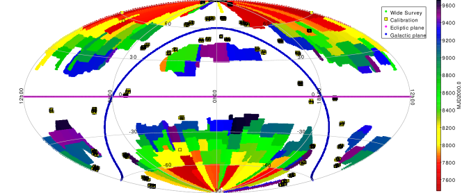
Figure 1: Expected coverage of the Euclid Wide survey (called the reference survey), color-coded by observing epoch, in an Aitoff projection of ecliptic coordinates. The horizontal gap corresponds to low ecliptic latitudes (the cyan line represents the ecliptic plane), and the circular gap to low galactic latitudes (the deep blue line stands for the galactic plane). The black squares filled with yellow are the calibration fields, repeatedly observed over the six years of the mission, to assess the stability and accuracy of Euclid point-spread function (PSF), photometry, and spectroscopy.

Euclid imaging detection limits are required at m${}_{\textrm{AB}}$ = 24.5 (10 $\sigma$ on a 1″ extended source) with VIS, and m${}_{\textrm{AB}}$ = 24 (5 $\sigma$ point source) in the Y, J, and H filters with NISP. Spectroscopic requirements are to cover the same near-infrared wavelength range at a resolving power of 380 and to detect at 3.5 $\sigma$ an emission line at $3.10^{-16}$ erg.cm^-1.s^-1 (on a 1″ extended source). The NISP implementation consists in two grisms, red (1.25 to 1.85 $\mu$m) and blue (0.92 to 1.25 $\mu$m, which usage will be limited to the Deep Survey), providing a continuum sensitivity to m${}_{\textrm{AB}}$ $\approx$ 21. To achieve these goals, the following survey operations were designed:

1. The observations will consist in a step-and-stare tiling mode, in which both instruments target the common 0.57 deg² field of view before the telescope slews to other coordinates.

2. Each tile will be visited only once, with the exception of the Deep Survey in which each tile will be pointed 40 times, and the calibration fields, observed 5 times each on average.

3. The filling pattern of the survey will follow lines of ecliptic longitude at quadrature. Current survey planning foresees a narrow distribution of solar elongation of $\Psi$ = 91.0 $\pm$ 1.5° only, the range of solar elongation available to the telescope being limited to 87°–110°.

4. The observation of each tile will be sub-divided in four observing blocks, differing only by small jitters (100″ $\times$ 50″). These small pointing offsets will allow to fill the gaps between the detectors composing each instrument focal plane, resulting in 95% of the sky covered by three blocks, and 50% by four.

5. In each block, near-infrared slitless spectra will be obtained with NISP simultaneously to a visible image with VIS, with an integration time of 565 s. This integration time implies a saturation limit of V${}_{\textrm{AB}}$$\approx$17 for a point-like source. Then, three NISP images will be taken with the Y, J, and H near-infrared filters, with integration time of 121, 116, and 81 s respectively (Fig. 2) .

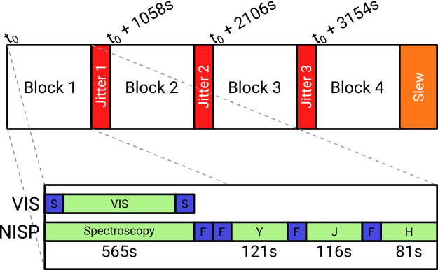
Figure 2: Observation sequence for each pointing. The observing block composed by a simultaneous VIS and NISP/spectroscopy exposure, and three NISP/imaging exposures (Y, J, H) is repeated four times, with small jitters (100″ $\times$ 50″). Blue boxes F and S stand for overheads due to the rotation of the filter wheel and shutter opening/closure. Figure adapted from Laureijs et al. (2011)

All these characteristics make Euclid a potential prime data set for legacy science. In particular, the access to the near-infrared sky, about 7 magnitudes fainter than DENIS and 2MASS (Epchtein et al., 1994; Skrutskie et al., 2006) surveys, and 2–3 magnitudes fainter than current ESO VISTA Hemispherical Survey (VHS, McMahon et al., 2013), makes Euclid appealing for surface characterization of Solar System Objects (SSOs), especially in an era rich in surveys operating in visible wavelengths only such as the Sloan Digital Sky Survey (SDSS), Pan-STARRS, ESA Gaia, and the Large Synoptic Sky Survey (LSST) (Abazajian et al., 2003; Jewitt, 2003; Gaia Collaboration et al., 2016; LSST Science Collaboration et al., 2009).
We discuss here the potential of the Euclid mission for Solar System Science. In the following, we consider the following populations of SSOs, defined by their orbital elements (Appendix A):

• the near-Earth asteroids (NEAs), including the Aten, Apollo, and Amor classes, which orbits cross that of terrestrial planets;

• the Mars-crossers (MCs), a transitory population between the asteroid main belt and the near-Earth space;

• the main-belt asteroids (MBA), in the principal reservoir of asteroids in the Solar System, between Mars and Jupiter, split into Hungarian, Inner Main-Belt (IMB), Middle Main-Belt (MMB), Outer Main-Belt (OMB), Cybele, and Hilda;

• the Jupiter trojans (Trojans), orbiting the Sun at the Lagrange L4 and L5 points of the Sun-Jupiter system;

• the Centaurs, which orbits cross that of giant planets;

• the Kuiper-belt objects (KBOs), further than Neptune, divided into Detached, Resonant, and Scattered-Disk Objects (SDO), and Inner, Main, and Outer Classical Belt (ICB, MCB, OCB); and

• the comets, from the outskirts of the solar system, on highly eccentric orbits, and characterized by activity (presence of coma) at short heliocentric distances.

The discussion is organized as following: the expected number of observation of Solar System Objects by Euclid is presented in Section 2, and their challenges in Section 3. The issue of source identification, and contribution to astrometry and orbit determination is discussed in Section 4. Then the potential for spectral characterization from VIS and NISP photometry is detailed in Section 5, and from NISP spectroscopy in Section 6. Euclid capabilities to directly image satellites and activity of SSOs are presented in Section 7, and its contribution to 3-D shape and binarity modeling from lightcurves in Section 8.

2 Expected number of SSO observations

Although Euclid Wide survey will avoid the ecliptic plane (Fig. 1), its design is casually very much adapted to detect moving objects. As described above, each FoV will be imaged 16 times in one hour, in four repeated blocks. Given the pixel scale of VIS and NISP cameras of 0.1″ and 0.3″, any SSO with an apparent motion larger than $\approx$0.2″/h should therefore be detected by its trailed appearance and/or motion across the different frames (Fig. 3).

Figure 3: Examples of the contamination of Euclid field of view by SSOs. Left: Survey field #15117 centered on (RA,Dec) = (167.218°,+12.740°) and starting on 2022, June the 16${}^{\textrm{th}}$ at 20:26:05 UTC. The successive trails impressed by the 6 known SSOs during the Euclid hour-long sequence of VIS-NISP imaging observations are drawn in different colors, one for each filter (VIS, Y, J, and H). We can expect about a hundred times more SSOs at Euclid limiting magnitude (e.g., Fig. 4). The inset is a magnified view of 2014 WQ501, a main-belt asteroid, illustrating the highly elongated shape of SSO in Euclid frames. The scale bar of 6″ corresponds to 60 pixels in VIS frames and 20 pixels in NISP. The timings reported are the starting time of VIS exposures. The slitless spectra will be acquired by NISP simultaneously to the VIS images. Right: Calibration field #13165 centered on (RA,Dec) = (76.785°,+23.988°) and starting on 2022, March the 9${}^{\textrm{th}}$ at 20:37:37 UTC. There are 117 known SSOs in the field, and here also, a hundred times more SSOs shall be detected at Euclid limiting magnitude.

To estimate the number of SSOs that could be detected by Euclid, we first build the cumulative size distribution (CSD) of each population. We use the absolute magnitude H as a proxy for the diameter $D$. The relation between both being $D(\textrm{km})=1329p_{V}^{-1/2}10^{-0.2H}$ (e.g., Bowell et al., 1989), where $p_{V}$ is the albedo of the surface in V, which quantifies its capability to reflect light. Minor planets, especially asteroids, tend to be very dark, and their albedo is generally very low, from a few percents to $\approx$30% (see, e.g., Mainzer et al., 2011).
We retrieve the absolute magnitude from the astorb database (Bowell et al., 1993), with the exception of comets, not listed in astorb, for which we use the compiled data by Snodgrass et al. (2011). The challenge is then to extrapolate the observed distributions (shown as solid lines in Fig. 4) to smaller sizes. Most are close to power-law distributions (Dohnanyi, 1969) in the form $dN/dH\propto 10^{\gamma H}$, with different slope $\gamma$. In the following, we model each population as following, and represent them with dashed lines in Fig. 4:

• NEAs: We use the synthetic population by Granvik et al. (2016) which is very similar to the one by Harris & D’Abramo (2015). We, however, take a conservative approach and increase the uncertainty of the model to encompass both estimates.

• MCs: There is no dedicated study of the CSD of MCs in the literature. We thus take the NEA model above, scaled by a factor of three to match currently known MC population. The upper estimate is taken as a power-law fit to current population with $\gamma$=0.41, and the lower estimate is the scaled NEA model by Granvik et al. (2016), reduced by a factor of two.

• MBAs: We use the knee distribution by Gladman et al. (2009), in which large objects (H $\in$ [11,15]) follow a steep slope ($\gamma\sim 0.5$) while smaller asteroids follow a shallower slope of $\gamma=0.30\pm 0.02$ in the range H $\in$ [15, 18], after which no constrain is available. This model is scaled to 25 954 asteroids at H = 15. These authors found the CSD to be very smooth in that absolute magnitude range, compared to earlier works (Jedicke & Metcalfe, 1998; Ivezić et al., 2001; Wiegert et al., 2007). We only slightly modify their model, changing the slope at H=15.25 instead of H=15: the shallower slope does not fit the observed data below H=15.25 anymore. The observing strategy by Gladman et al. (2009) was indeed aimed at constraining the faint end of the CSD, and the constraints on large bodies was weak (only a small sky area had been targeted).

• Trojanss: We use the model of Jewitt et al. (2000), with $\gamma=0.4\pm 0.06$. More recently, Grav et al. (2011) found a similar $\gamma$, but restricted their study to Trojans with $D>10$ km. We scale their model to the number of 310 known Trojans at H = 12.5. The steeper slope (i.e., $\gamma=0.46$) seems to reproduce more accurately current observed population. The baseline numbers for Trojan presented here may therefore be underestimated, and the upper estimate could represent better the real Trojan population. Finally, we do not use the knee model by Yoshida & Nakamura (2005), who predicted a change of slope at D$\approx$5 km, because their model does not fit the known population anymore.

• Centaurs: We use the $\gamma=0.34\pm 0.04$ from Bauer et al. (2013), which is close from the 0.4 estimate from Jedicke et al. (2002). We scale the power-law to correspond to the cumulative population (7) at H = 8.25.

• KBOs: First, we build the CSD of the Resonant population using a single power-law of index $\gamma=0.9_{-0.4}^{+0.2}$, scaled to a total of 22,000 objects a H = 8.66, proposed by Volk et al. (2016) based on the early results of the Outer Solar System Origins Survey (OSSOS, Bannister et al., 2016) which is consistent with the earlier work by Gladman et al. (2012) based on the Canada-France Ecliptic Plane Survey (CFEPS). Then, we build the CSD of the Scattered-disk objects using the divot distribution by Shankman et al. (2016): large objects follow a steep slope ($\gamma\sim 0.9$), scaled to a total of 6500 objects a H = 8, which changes at H = 8.0 to a shallower $\gamma=0.50_{-0.08}^{+0.15}$. The differential size distribution present a drop at H = 8.0 where the slope changes, the smaller objects being less numerous by a factor of 5.6 (see Shankman et al., 2016, for details). Finally, we take the CSD of objects in the Classical Belt from Petit et al. (2016) which propose a knee distribution: $\gamma=1.02$, scaled to a total of 1800 objects at H = 7, until H=7.0 (in agreement with Adams et al., 2014) where it switches to $\gamma=0.65\pm 0.05$. The CSD for the entire KBO population is the sum of the three aforementioned CSD.

• Comets: We use the knee CSD from Snodgrass et al. (2011). Largest comets follow an $\gamma=0.38_{-0.04}^{+0.06}$ until H = 17 (converted from the turnover radius of 1.25 km using an albedo of 0.04) after which the CSD is shallower, although less constrained, and we assume the average slope found by Snodgrass et al. (2011) with arbitrary uncertainties: $\gamma=0.04_{-0.02}^{+0.06}$.

Figure 4: Cumulative size distribution of each SSO population, for current census (solid lines) and synthetic populations (average estimates represented by the dashed lines, upper and lower estimate not plotted for clarity). The number of known objects, observable at Euclid limiting apparent magnitude over the entire celestial sphere, are represented by the dot-dashed lines. The open squares and circles represent the 0-25-50-75-100% marks of the (H-V) cumulative probability function at the saturation and photon-starving ends. The total number of objects expected on the sky are marked by the filled circles. The difference between these filled circles and the current census represents the margin for discovery.

The question is then what range of absolute magnitude will be accessible to Euclid for each population, considering it will observe in the range V${}_{\textrm{AB}}$ = 17–24.5. This conversion from apparent to absolute magnitude only depends on the geometry of observation (Bowell et al., 1989) through the heliocentric distance ($\Delta$), range to observer ($r$), and phase angle ($\alpha$, the angle between the target-Sun and target-observer vectors):

$$H=V+2.5\log\Big{(}r^{2}\Delta^{2}\Big{)}-2.5\log\Big{(}(1-G)\phi_{1}+G\phi_{2}\Big{)}$$ (1)

with the phase functions approximated by

$$\phi_{1} = \exp\left(\ -3.33\tan\left(\frac{\alpha}{2}\right)^{0.63}\right)$$ (2)

$$\phi_{2} = \exp\left(\ -1.87\tan\left(\frac{\alpha}{2}\right)^{1.22}\right)$$ (3)

Although a more accurate model (with two phase slopes $G_{1}$ and $G_{2}$) of the phase dependence has been developed recently (Muinonen et al., 2010), the differences in the predicted magnitudes between the two systems are minor for our purpose. We thus use the former and simplier H-G system in the following, assuming the canonic value of $G=0.15$.
The three geometric parameters ($r$,$\Delta$,$\alpha$) are tight together by the solar elongation $\Psi$, which is imposed by the spacecraft operations ($\Psi$ = 91.0 $\pm$ 1.5°). In practice, it is sufficient to estimate the range of heliocentric distances at which Euclid will observe an SSO from a given population to derive the two other geometric quantities, and hence the (H-V) index:

$$r = \cos{\Psi}+\sqrt{\cos^{2}{\Psi}-1+\Delta^{2}.}$$ (4)

$$\alpha = \left|\operatorname{asin}\left(\frac{\sin\Psi}{\Delta}\right)\right|$$ (5)

Table 1: Expected number of SSOs observed by Euclid for each population. For the whole celestial sphere, we report the current number of known SSOs ($\mathcal{N}$${}_{\textrm{now}}$, at the time of the writing on 2017 June 28), the expected number of objects observable ($\mathcal{N}$${}_{\textrm{S}}$) at Euclid limiting apparent magnitude (V${}_{\textrm{AB}}$$<$24.5) and solar elongation ($\Psi$ = 91.0 $\pm$ 1.5°). Using the fraction of known SSOs present within the area of the Euclid Wide survey ($f_{W}$) and calibration frames ($f_{C}$), we estimate total number of discoveries ($\mathcal{N}$${}_{\textrm{E,d}}$) and observations ($\mathcal{N}$${}_{\textrm{E,o}}$) by Euclid. The absolute magnitude corresponding to a probability of 100%, 50%, and 1% that SSOs will be within Euclid detection envelop are also reported.

Population		All-Sky	$f_{W}$	$f_{C}$	Euclid		Absolute magnitude limits
Name	$\mathcal{N}$${}_{\textrm{now}}$	$\mathcal{N}$${}_{\textrm{S}}$	(%)	(%)	$\mathcal{N}$${}_{\textrm{E,d}}$	$\mathcal{N}$${}_{\textrm{E,o}}$	H${}_{\textrm{100}}$	H${}_{\textrm{50}}$	H${}_{\textrm{1}}$
NEA	16062	$1.9_{-0.6}^{+1.1}\times 10^{5}$	$7.2\pm 0.4$	$0.8\pm 0.1$	$1.4_{-0.5}^{+1.0}\times 10^{4}$	$1.5_{-0.6}^{+1.0}\times 10^{4}$	22.75	23.75	26.50
MC	15488	$1.2_{-0.8}^{+1.6}\times 10^{5}$	$9.0\pm 0.6$	$0.6\pm 0.1$	$1.0_{-0.8}^{+1.7}\times 10^{4}$	$1.2_{-0.8}^{+1.7}\times 10^{4}$	21.00	21.25	22.75
MB	674981	$4.3_{-0.9}^{+1.0}\times 10^{6}$	$1.5\pm 0.0$	$0.7\pm 0.0$	$8.2_{-2.2}^{+2.5}\times 10^{4}$	$9.7_{-2.2}^{+2.5}\times 10^{4}$	19.50	20.00	21.25
Trojan	6762	$1.3_{-0.7}^{+0.9}\times 10^{5}$	$5.1\pm 1.5$	$0.5\pm 0.4$	$7.1_{-4.9}^{+9.3}\times 10^{3}$	$7.5_{-5.0}^{+9.5}\times 10^{3}$	17.00	17.25	18.25
Centaur	470	$1.8_{-1.0}^{+1.4}\times 10^{4}$	$12.2\pm 0.9$	$0.6\pm 0.4$	$2.2_{-1.4}^{+2.1}\times 10^{3}$	$2.2_{-1.4}^{+2.1}\times 10^{3}$	14.75	15.50	18.25
KBO	2331	$9.8_{-1.9}^{+2.2}\times 10^{4}$	$4.9\pm 0.2$	$0.6\pm 0.1$	$5.3_{-1.3}^{+1.6}\times 10^{3}$	$5.5_{-1.3}^{+1.6}\times 10^{3}$	8.25	8.75	10.00
Comet	1301	$185.2_{-13.5}^{+15.4}$$\times 10^{0}$	$19.5\pm 0.5$	$1.0\pm 0.3$	$21.5_{-3.6}^{+4.2}$$\times 10^{0}$	$38.2_{-4.3}^{+4.9}$$\times 10^{0}$	18.25	19.00	22.00
Total	717395	$4.9_{-1.2}^{+1.4}\times 10^{6}$	$2.1\pm 0.1$	$0.7\pm 0.0$	$1.2_{-0.4}^{+0.7}\times 10^{5}$	$1.4_{-0.4}^{+0.7}\times 10^{5}$

We thus compute the probability density function (PDF) of the heliocentric distance of each population. For that, we compute the 2-D distribution of the semi-major axis vs eccentricity of each population using bins of 0.05 in AU and eccentricity. For each bin, we compute the PDF of heliocentric distance from Kepler’s second law. We then sum individual PDF from each bin, normalized by the number of SSO in each bin divided by the entire population.
We then combine the distribution of solar elongation from the reference survey and the PDF of heliocentric distance of each population in Eqs. 4 and 5 to obtain a PDF of the (H-V) index (Eq. 1). The fraction of populations to be observed by Euclid at each magnitude is estimated by multiplying the CSD of the synthetic populations with the cumulative distribution of the (H-V) index, at both ends of Euclid magnitude range (V${}_{\textrm{AB}}$ = 17–24.5, see the dot-dashed lines in Fig. 4). The number of SSOs observable on the entire celestial sphere ($\mathcal{N}$${}_{\textrm{S}}$) can be simply read on this graph, and are reported in Table 1. The difference between synthetic and observed population also provides an estimate of the potential number of objects to be discovered by Euclid down to V${}_{\textrm{AB}}$ = 24.5.
We then estimate how many of these objects will be observed by Euclid. For that, we compute the position of all known SSOs every six months for the entire duration of Euclid operations (2020 to 2026) by using the Virtual Observatory (VO) web service SkyBot 3-D (Berthier et al., 2008). This allows to compute the fraction of known SSOs present within the area covered by Euclid surveys ($f_{W}$, $f_{D}$, and $f_{C}$ for the Wide and Deep surveys, and calibration frames). We report these fraction in Table 1, except $f_{D}$ which is negligible (of the order of 1-10 ppm) due to the low number of known SSOs on highly inclined orbits (although there is a clear bias against discovering such objects in current census of SSOs, see Petit et al., 2017; Mahlke et al., 2017). These figures are roughly independent of the epoch for all populations but for the Trojans, which are confined around Lagrangian L4 and L5 points on Jupiter’s orbit and therefore cover a limited range in right ascension at each epoch.
Overall, about 150,000 SSOs are expected to be observed by Euclid, in a size range currently unexplored by large surveys. This estimate could be refined once dedicated studies of the detection envelop of moving objects will be performed on simulated data. Euclid could discover thousands of outer solar system objects and tens of thousands of sub-kilometric main-belt, Mars-crosser, and near-Earth asteroids (see typical absolute magnitudes probed by Euclid in Table 1). Nevertheless, the Large Synoptic Survey Telescope (LSST, LSST Science Collaboration et al., 2009) is expected to have its scientific first-light in 2021. The LSST will repeatedly image the sky down to V$\approx$24, over a wide range of solar elongations, and will be a major discoverer of faint SSOs. Assuming a discovery rate of 10,000 NEAs, 10,000 MCs, 550,000 MBAs, 30,000 Trojans, 3000 Centaurs, 4000 KBOs, and 1000 comets per year (LSST Science Collaboration et al., 2009), most of the SSOs potentially available for discovery should be discovered by LSST in the southern hemisphere. Exploration of small KBOs in the northern hemisphere will however be specific of Euclid.

3 Specificity of Euclid observations of SSOs

The real challenge of SSO observations with Euclid will be the astrometry and photometry of highly elongated sources (as hinted by Fig. 3). We present in Fig. 5 and Table 2 a summary of the apparent non-sidereal rate of the different population of SSOs. With the exception of the distant-most populations of KBOs, Centaurs, and comets, all SSOs will present rates above 10″/h. This implies a motion of hundreds of pixels between the first and last VIS frame. During a single exposure, each SSO will move and produce a trailed signature, a streak, which length will typically range from 1 to 50 pixels for VIS. The situation will be more favorable for NISP, thanks to the shorter integration times and larger pixel scale, and most SSOs will not trail, or over a few pixels only (Table 2).
There have been some recent developments to detect streaks, motivated by the optical detection and tacking of artificial satellites and debris on low orbits around the Earth. Dedicated image processing for trails can be set up to measure the astrometry and photometry of moving objects within a field of fixed stars, without an a priori knowledge of their apparent motion (e.g., Virtanen et al., 2016). The success rate in detecting these trails has been shown to reach up to 90%, even in low signal-to-noise ratio ($\approx$1) regime. Such algorithms are currently being tested on simulated Euclid data of SSOs (M. Granvik, personal communication).

Table 2: For each main population of SSOs, we report the apparent rate and its 25% and 75% quartile variations (i.e., half the population is within these two values), and the length of the trails on the detector during the simultaneous VIS imaging and NISP spectroscopic 565 s exposure, and the following NISP Y, J, and H imaging exposures of 121, 116, and 81 s.

Population	Rate	VIS	NISP	Y	J	H
	(″/h)	(pix)	(pix)	(pix)	(pix)	(pix)
NEA	43.3${}_{\scriptscriptstyle-19.9}^{\scriptscriptstyle+36.5}$	67.9	22.6	4.8	4.6	3.2
MC	41.3${}_{\scriptscriptstyle-14.9}^{\scriptscriptstyle+22.6}$	64.8	21.6	4.6	4.4	3.1
MB	32.5${}_{\scriptscriptstyle-5.5}^{\scriptscriptstyle+7.9}$	51.0	17.0	3.6	3.5	2.4
Trojan	13.3${}_{\scriptscriptstyle-1.1}^{\scriptscriptstyle+1.4}$	20.9	7.0	1.5	1.4	1.0
Centaur	4.0${}_{\scriptscriptstyle-1.5}^{\scriptscriptstyle+2.9}$	6.2	2.1	0.4	0.4	0.3
KBO	0.6${}_{\scriptscriptstyle-0.1}^{\scriptscriptstyle+0.3}$	1.0	0.3	0.1	0.1	0.0
Comet	4.4${}_{\scriptscriptstyle-1.8}^{\scriptscriptstyle+6.2}$	6.9	2.3	0.5	0.5	0.3

Figure 5: Five-number summary (minimum, maximum, median, 25% and 75% quartiles) of the apparent rate of each population of SSOs. The Euclid mode of observation at quadrature reduces the apparent rate compared to, e.g., opposition.

4 Source identification, astrometry, and dynamics

As established in Section 2, Euclid will observe of the order of 150,000 SSOs, even if its nominal survey is avoiding ecliptic latitudes below 15°, with the notable exception of the calibration fields (Fig. 1).
The design of the surveys, with hour-long sequences of observation of each field, will however preclude orbit determination for newly discovered objects. This hour-long coverage is nevertheless sufficient to discriminate between NEAs, MBAs, and KBOs (Spoto et al., 2017). The situation will be very similar to the SDSS Moving Object Catalog (MOC), in which many SSO sightings corresponded to unknown objects at the time of the release (still about 53% at the time of the 4${}^{\textrm{th}}$ release, Ivezić et al., 2001, 2002). Attempts for identification will have to be regularly performed a posteriori once the number of known objects, hence orbits, will increase, like we did for the SDSS MOC, identifying 27% of the unknown sources (Carry et al., 2016), using the SkyBoT Virtual Observatory tool (Berthier et al., 2006, 2016). The success rate for a posteriori identification of SSOs detected by Euclid should even be higher than in aforementioned study, as the LSST will be sensitive to the same apparent magnitude range.
Compared with tens of points over many years provided by the LSST, the astrometry by Euclid should contribute little to the determination of SSO orbits, with the following exceptions. First, the objects in the outer solar system (Centaurs and KBOs) in the northern hemisphere will not be observed by LSST. In this respect, the Deep survey will allow to study the population of highly inclined Centaurs and KBOs (e.g., Petit et al., 2017), thanks to the repeated observations of the northern Ecliptic cap (about 40 times). Second, the parallax between the Earth and the Sun-Earth L2 point is large, from about a degree for asteroids in the inner belt, to a few tens of arcseconds for KBOs. Simultaneous observation of the same field from the two locations thus provides the distance of the SSO, reducing drastically the possible orbital parameters space (Eggl, 2011). Thus, an interesting synergy between LSST and Euclid would reside in planning these simultaneous observations (see, Rhodes et al., 2017). The practical implementation may however be difficult as the observations by Euclid at a solar elongation $\Psi$ of 91.0 $\pm$ 1.5° impose observations close to sunset or sunrise from LSST.

5 Photometry and spectral classification

Figure 6: Examples of asteroids classes (A, L, S, and V) which are degenerated over visible wavelength range. For reference, the wavelength coverage of each photometric filter and grism on-board Euclid is shown, together with SDSS and LSST set of filters (u, g, r, i, z, Ivezić et al., 2001), 2MASS and VISTA, and Gaia blue and red photometers (BP, RP) that will produce low-resolution spectra (resolving power of a few tens, Delbo et al., 2012).

In this section we study the impact of Euclid on spectral classification of SSOs, thanks to the determination of their spectral energy distribution (SED, see Appendix B) over a large wavelength range, from the visible with VIS (0.5 $\mu$m) to the near-infrared with NISP (2 $\mu$m). While colors in the visible have been and will be obtained for several 10⁶ SSOs thanks to surveys like ESA Gaia and the LSST (Gaia Collaboration et al., 2016; LSST Science Collaboration et al., 2009), collection of near-infrared photometry is lacking. The only facility currently operating from which near-infrared colors for numerous SSOs have been obtained is the ESO VISTA telescope (Popescu et al., 2016). As described above, the upcoming ESA Euclid (and also the NASA WFIRST mission which shares many specifications with Euclid, see Green et al., 2012; Holler et al., 2017) may radically change this situation.
At first order, SSOs display a G2V spectrum at optical wavelength, due to the reflection of the Sun light by their surface. Depending on their surface composition, regolith packing, and degree of space weathering, their spectra are however modulated by absorption bands and slope effects. Historically, SSOs spectra have always been studied in reflectance, that is their recorded spectrum divided by the spectrum of the Sun, approximated by a G2V star observed with the same instrument setting as the scientific target. The colors and low-resolution (R $\approx$ 300-500) of asteroids have been used since decades to classify them, in a scheme called taxonomy, using the visible range only, or the near-infrared only, or both (see, Chapman et al., 1975; Barucci et al., 1987; Bus & Binzel, 2002b, a; DeMeo et al., 2009). For KBOs, broad-band colors and medium-resolution (R$\approx$3000–5000) have been used to characterize their surface composition (e.g., Snodgrass et al., 2010; Carry et al., 2011, 2012), although current taxonomy is based on broad-band colors only (Fulchignoni et al., 2008).

Figure 7: The eleven asteroid (A- to X-type) and four KBO (BB, BR, IR, RR) spectral classes considered here, converted into photometry for classification simulation (see text). The transmission curves of VIS and NISP filters are also plotted for reference.

Information on the taxonomic class has been derived for about 4000 asteroids based on their low-resolution spectra (mainly from SMASS, SMASSII, and S³OS² surveys, see Bus & Binzel, 2002b, a; Lazzaro et al., 2004). Using the broad-band photometry from the Sloan Digital Sky Survey (SDSS), many studies have classified tens of thousands of asteroids (e.g., Ivezić et al., 2001, 2002; Nesvorný et al., 2005; Carvano et al., 2010; DeMeo & Carry, 2013). These studies opened a new era in the study of asteroid families (Carruba et al., 2013), space weathering (Nesvorný et al., 2005; Thomas et al., 2012), distribution of material in the inner solar system (DeMeo & Carry, 2014; DeMeo et al., 2014), and origins of near-Earth asteroids (Carry et al., 2016). The on-going survey by ESA Gaia will provide low-resolution spectra (R$\approx$35) for 300,000 asteroids, with high photometric accuracy, and the taxonomic class will be determined for each SSO (Delbo et al., 2012).
Nevertheless, any classification based on SDSS, Gaia, or LSST (which will use a filter set comparable with SDSS), suffers from a wavelength range limited to the visible only. It is, however, known that several classes are degenerated over this spectral range, and only near-infrared colors/spectra can disentangle them (Fig. 6 and DeMeo et al., 2009). The near-infrared photometry provided by Euclid will therefore be highly valuable, alike that reported from 2MASS (Sykes et al., 2000) or ESO VISTA VHS (McMahon et al., 2013; Popescu et al., 2016) surveys.
To estimate the potential of Euclid photometry for spectral classification of asteroids, we simulate data using the visible and near-infrared spectra of the 371 asteroids that were used to create the Bus-DeMeo taxonomy (DeMeo et al., 2009), and of 43 KBOs with known taxonomy (Merlin et al., 2017). We convert their reflectance spectra into photometry (Fig. 7), taking the reference VIS and NISP filter transmission curves .

Figure 8: Result of the classification of the 371 asteroids from Bus-DeMeo taxonomy, presented in three filter combinations: VIS-Y, VIS-J, and Y-H. Several extreme classes, like A, B, D, V, and T, can be easily sorted out thanks to the large wavelength coverage of Euclid.

One key aspect of Euclid operations for determining the colors of SSO is the repetition of the four-filters sequence over an hour. Thus, each filter will be bracketed by other filters in time. This will allow to determine magnitude difference between each pair of filters without biases otherwise introduced by the intrinsic variation of the target (Appendix B). For a detailed discussion on that effect, see Popescu et al. (2016).
For each class and combination of filter, we compute the average color, dispersion, and co-variance. This allows to classify objects based on their distance to all the class centers, normalized by the typical spread of the class (Pajuelo, 2017). This learning sample is of course limited in number, and all classes are not evenly represented. It nevertheless allows to estimate Euclid capabilities by applying the classification scheme to the same sample. This is presented in Fig. 8. The leverage provided by the long wavelength coverage allows to clearly identify several classes: A, B, D, V, Q, and T (DeMeo et al., 2009). The main classes in the asteroid belt, the C, S, and X (DeMeo & Carry, 2014), are more clumped, and our capabilities to classify them will depend on the exact throughput of Euclid optical path.

Figure 9: Percentage of correct (solid bar) and compatible (open bar) classification for each Bus-DeMeo taxonomic classes. The Euclid photometry alone allows to classify asteroids into 11 classes.

For KBOs, their spectral behavior from the blue-ish BB to the extremely red RR will place them in these graphs along a line going though the C, T, and D-types (which colors are close to the BB, BR, and IR classes). The RR-types will be even further from the central clump than the D-types. Identifying the different KBO spectral classes should therefore be straightforward with Euclid set of filters.
In all cases, spectral characterization using Euclid colors will benefit from the colors and spectra in the visible observed by Gaia and LSST (Delbo et al., 2012; LSST Science Collaboration et al., 2009), visible albedo (from IRAS, AKARI, WISE, Herschel observations, e.g., Tedesco et al., 2002; Müller et al., 2009; Masiero et al., 2011; Usui et al., 2011), and solar phase function parameters (see Oszkiewicz et al., 2012, for an example of the use of phase function for taxonomy). The success rate of classification from Euclid photometry only hence represents a lower estimate.
We present in Fig. 9 the success rate of classification of the 371 asteroids from the Bus-DeMeo taxonomy. The classes are generally recovered with a success rate above 60%, and when misclassified, asteroids end up in spectrally similar (compatible) classes with a success rate closer to 90%, but for the C and X classes. We do not repeat the exercise for KBOs given the limited size of the available sample. Their spectral classes being, however, much alike the C, T, and D-type asteroid, and even redder, their identification should be straightforward with Euclid filter set.
In summary, the VIS and NISP photometry that will be measured by Euclid seems very promising to class SSOs among their historical spectral classes.

6 Near-infrared spectroscopy with NISP

Euclid will also acquire near-infrared low-resolution (resolving power of 380) spectra for many SSOs, down to m_AB $\approx$ 21, i.e., similar to Gaia limiting magnitude. Simultaneously to the four VIS exposures, NISP will acquire four slitless spectra of the same field of view. In the wide survey, only the red grism (1.25 to 1.85 $\mu$m) will be used, the usage of the blue grism (0.92 to 1.25 $\mu$m) being limited to the deep survey. The red grism will cover typical absorption bands of volatile compounds (e.g., water or methane ices) such as found on distant KBOs. The main diagnostic features of asteroids (NEAs, MBAs) are however located within the blue arm at 1 $\mu$m, and at 2 $\mu$m, outside the spectral range of the red grism.
Because there is no slit, many sources will be blended. To decontaminate each slitless spectrum from surrounding sources, the exposures will be taken with three different grism orientations, 90° apart. For exposures with the spectral dispersion aligned with the ecliptic, i.e., parallel to the typical SSO motion, as each SSO will blend with itself. For the remaining orientations, SSOs will often blend with background sources, degrading both spectra. This may be an issue for the wide survey in its lowermost ecliptic latitude range, where many sources will be blended with G2V spectra from SSOs.
The apparent motion of outer solar system objects being limited (Table 2), their spectra may be extracted by the Euclid consortium tools, designed to work on elongated sources (typically 1″). Near-infrared spectra for thousands of Centaurs and KBOs could thus be produced by Euclid. For objects in the inner solar system, the extraction of their spectra may be challenging, and in-depth assessment of the feasibility of such measurements is beyond the scope of this paper. In both cases, these spectra be very similar to the low-resolution spectra used to define current asteroid taxonomy (DeMeo et al., 2009) and diagnostic of KBOs class as defined by (Fulchignoni et al., 2008).

7 Multiplicity and activity of SSOs

With a very stable PSF and a pixel scale of 0.1″ and 0.3″ for VIS and NISP, close to the diffraction limit of Euclid, the morphology of sources can be studied. This is indeed one of the main goals of the cosmological survey (Laureijs et al., 2011). We first assess how Euclid could detect satellites around SSOs, and then activity, i.e., dust trails.

7.1 Direct imaging of multiple systems with Euclid

In two decades since the discovery of the first satellite of asteroids, Dactyl around (243) Ida, by the Galileo mission (Chapman et al., 1995), direct imaging has been the main source of discovery and characterization of satellites around large SSOs, in the main belt (e.g., Merline et al., 1999; Berthier et al., 2014), among Jupiter Trojans (Marchis et al., 2006, 2014), and KBOs (e.g., Brown et al., 2005, 2006, 2010; Carry et al., 2011; Fraser et al., 2017). This is particularly evident for KBOs, for which 65 of the 80 known binary systems where discovered by the Hubble Space Telescope, and the other 14 by large ground-based telescopes, often supported by adaptive optics (see, e.g., Parker et al., 2011; Johnston, 2015; Margot et al., 2015). The situation is different for NEAs and small MBAs, for which most discoveries and follow-up observations were made with optical lightcurves and radar echoes (e.g., Pravec & Harris, 2007; Pravec et al., 2012; Fang et al., 2011; Brozović et al., 2011).
To estimate Euclid capabilities to angularly resolve a multiple system, we use the compilation of system parameters by Johnston (2015). We compute the magnitude difference between components $\Delta m$ from their diameter ratio, and their typical separation $\Theta$ from the ratio of the binary system semi-major axis to its heliocentric semi-major axis (Table 3).

Table 3: Typical magnitude difference ($\Delta m$) and angular separation ($\Theta$) between components of multiple SSO systems. NEA and MCs share similar characteristics, and so does large MBAs and Trojans. We split MBAs into two categories, according to the diameter $D$ of the main component. Estimates on the frequency of binaries in each populations are based on the reviews by Noll et al. (2008) and Margot et al. (2015). We only consider high-inclination KBOs here, the fraction of binaries in the cold belt being closer to 30% (Fraser et al., 2017).

Population	$\Delta m$	$\Theta$	$f$
	(mag)	(″)	(%)
NEA & MC	$1.8_{-1.8}^{+2.0}$	$0.01_{-0.01}^{+0.01}$	$15\pm 5$
MBA ($D<10$ km)	$2.5_{-0.9}^{+0.9}$	$0.01_{-0.01}^{+0.01}$	$15\pm 5$
MBA ($D>100$ km)	$5.4_{-2.7}^{+2.7}$	$0.30_{-0.25}^{+0.25}$	$3\pm 2$
KBO	$1.5_{-1.5}^{+2.0}$	$0.43_{-0.43}^{+0.60}$	$6\pm 4$

The angular resolution of Euclid will thus allow to detect satellites of KBOs and large MBAs, but not those around NEAs, MCs, and small MBAs. The case of KBOs is straightforward, owing to the very little smearing of their PSF from their apparent motion (Table 2). Based on the expected number of observations of KBOs (Table 1) and their binarity fraction, Euclid should observe 300 $\pm$ 200 multiple KBO systems, i.e., a four fold increase.
The case of MBAs is more complex. First, there are only 25 large MBAs with an inclination higher than 15°, i.e., potentially observable by Euclid. Second, the fraction and properties of multiple systems for MBAs with a diameter between 10 and 100 km is terra incognita. This is due to observational biases: detection by lightcurves is more efficient on close-by components, and direct imaging, especially from ground-based telescopes using adaptive optics, focused on bright, hence large, primaries. If most binaries around small asteroids ($D<10$ km) are likely formed by rotational fission caused by YORP spin-up (Walsh et al., 2008; Pravec et al., 2010; Walsh & Jacobson, 2015), satellites of larger bodies are the result of re-accumulation of ejecta material after impacts (Michel et al., 2001; Durda et al., 2004). Some satellites around mid-sized MBAs are therefore to be expected, but with unknown frequency. Considering a ratio of $\approx$5 between the semi-major axis of binary system and the diameter of the main component (typical of large MBAs, see Margot et al., 2015) and the size distribution of high-inclination MBAs, only a handful of potential systems would have separations angularly resolvable by Euclid. Finally, the apparent motion of MBAs implies highly elongated PSFs, diminishing even further the fraction of detectable systems.
For these reasons, Euclid will therefore contribute little, if at all, to the characterization of multiple systems among asteroids. Prospects for discoveries of KBO binaries is however very promising.

7.2 Detection of activity

The distinction between comets and other kind of small bodies in our Solar System is, by convention, based on the detection of activity, i.e., of unbound atmosphere also called coma. Comets cannot be distinguished from their orbital elements only (Fig. 12). The figure blurred further with the discovery of comae around Centaurs, and even MBAs, called active asteroids (see Jewitt, 2009; Jewitt et al., 2015, for reviews).
The cometary-like behavior of these objects was discovered either by sudden surges in magnitude, or diffuse non-point-like emission around them. There are currently 18 known active asteroids and 12 known active Centaurs, corresponding to 25 ppm and 13% of their host populations respectively. The property of the observed comae is typically 1 to 5 magnitude fainter than the nucleus, within a 3″ radius (although this large aperture was chosen to avoid contamination from the nucleus PSF which extended to about 2″ due to atmospheric seeing, Jewitt, 2009).
With much higher angular resolution, and its very stable PSF required for its primary science goal (Laureijs et al., 2011), Euclid has the capability to detect such activity. Based on the expected number of observations (Table 1) and the aforementioned fraction of observed activity, Euclid could observe a couple of active asteroids and about 300${}_{-200}^{+300}$ active Centaurs. As in the case of multiple systems however, detection capability will be diminished by the trailed appearance of SSOs. This will be dramatic for MBAs, but limited for Centaurs (Table 2): typical motion will be of 6 pixels, i.e., 0.6″, while typical coma extend over several arcseconds.

8 Time-resolved photometry

The observations of each field, in four repeated sequences of VIS and NISP photometry, will provide hour-long lightcurves sampled by 4 $\times$ 4 measurements, or a single lightcurve made of 16 measurements by converting all magnitudes from the knowledge of the SED (Fig. 10, Appendix B).

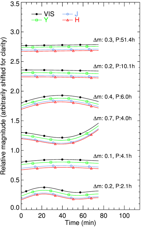
Figure 10: Examples of simulated SSO multi-filter lightcurves as observed by Euclid VIS and NISP. For each lightcurve, the amplitude ($\Delta m$) and rotation period (P) is reported. For each, the four lightcurves corresponding to the different filters are printed (with a magnitude difference reduced by a factor 10 for clarity), together with the photometry at the cadence of Euclid.

Since decades, optical lightcurves have been the prime data set for 3-D shape modeling and study of SSO multiplicity from mutual eclipses (see the reviews by Margot et al., 2015; Ďurech et al., 2015). Taken alone, a single lightcurve, such as those Euclid will provide, does not provide much constrains. Both shape and dynamical modeling indeed require multiple Sun-target-observer geometries, which can only be achieved by accumulating data over many years and oppositions.

8.1 Period, spin, and 3-D shape modeling

Traditionally, the period, spin orientation, and 3-D shape of asteroids were determined by using many lightcurves taken over several apparitions (e.g., Kaasalainen & Torppa, 2001; Kaasalainen et al., 2001). It has been show later on that photometry measurements, sparse in time, convey the same information and can be use alone or in combination with dense lightcurves (Kaasalainen, 2004). Large surveys such as Gaia and the LSST will deliver sparse photometry for several 10^5-6 SSOs (Mignard et al., 2007; LSST Science Collaboration et al., 2009).
In assessing the impact of PanSTARRS and Gaia data on shape modeling, Ďurech et al. (2005) and Hanuš & Ďurech (2012) however showed that searching for the rotation period with sparse photometry only may result in many ambiguous solutions. The addition of a single dense lightcurve often removes many aliases and harmonics in a periodogram, removing the ambiguous solutions, the impact of the single lightcurve depending on the fraction of the period it covers (J. Durech, personnal communication).

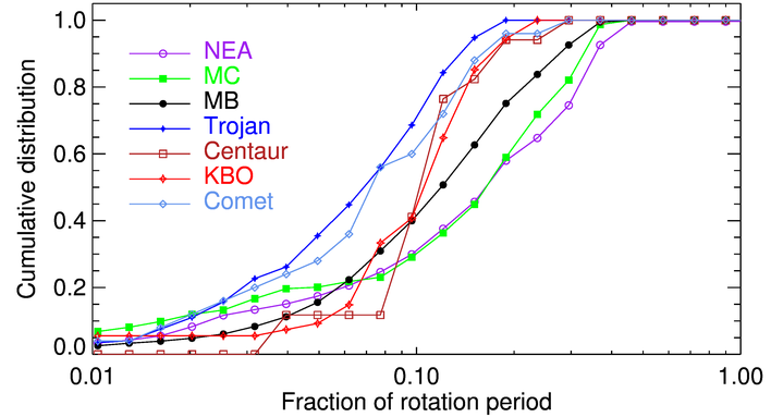
Figure 11: Cumulative distribution of the fraction of rotation covered by one hour of observations, computed on the 5759 entries with a quality code 2 or 3 from the Planetary Data System archive (Harris et al., 2017), and the 25 comets from Samarasinha et al. (2004) and Lowry et al. (2012).

The rotation periods of SSOs range from a few minutes to several hundreds of hours. The bulk of the distribution is however confined between 2.5 h (which is called the spin barrier, see e.g., Scheeres et al., 2015) and 10–15 h. This implies that Euclid lightcurves will typically cover between 5–10 and 40% of the rotation period of SSOs (Fig. 11). Euclid lightcurves will cover more than a quarter of rotation (the maximum change in geometry over a rotation, used here as a baseline) for 35% of NEAs, 28% of MCs, and 16% of MBAs, and only a handful of outer solar system objects The hour-long lightcurves provided by Euclid will thus be valuable for 3-D shape modeling of thousands of asteroids ($5.25_{-2.10}^{+3.50}\times 10^{3}$ NEAs, $3.36_{-2.24}^{+4.76}\times 10^{3}$ MCS, and $1.55_{-0.35}^{+0.40}\times 10^{4}$ MBAs).

8.2 Mutual events and multiplicity

Binary asteroids represent about 15 $\pm$ 5% of the population of NEAs larger than 300 m (Sect. 7, Pravec et al., 2006), and a similar fraction is expected among MCs and MBAs with a diameter smaller than 10 km (Table 3, Margot et al., 2015). Most of these multiple systems were discovered by lightcurve observations recording mutual eclipsing and occulting events (140 of the 205 binary asteroid systems known to date, the remaining being mostly binary NEAs discovered by radar echoes, see Johnston, 2015).
These systems have orbital periods of 24 $\pm$ 10 h, and diameter ratio of $0.33\pm 0.17$, which implies a magnitude drop of $0.11_{-0.08}^{+0.13}$ during mutual eclipses and occultations (computed from the compilation of the properties of binary systems by Johnston, 2015). The hour-long lightcurves provided by Euclid will thus typically cover 4${}_{-1}^{+3}$% of the orbital period. Considering the systems are in mutual events for about 20% of the orbital period at the high phase angle probed by Euclid (e.g., Pravec et al., 2006; Carry et al., 2015), there is a corresponding probability of $\approx$(5 $\pm$ 2)% to witness mutual events. Hence, Euclid could record mutual events for 900${}_{-450}^{+700}$ NEAs, MCs, and MBAs, helping characterizing these systems in combination with other photometric data sets such as those provided by Gaia and the LSST.

9 Conclusion

We have explored how the ESA mission Euclid can contribute to Solar System science. The operation mode of Euclid is by chance well designed for detection and identification of moving objects. The deep limiting magnitude (V${}_{\textrm{AB}}$ $\sim$ 24.5) of Euclid and large survey coverage (even if avoiding low ecliptic latitude) promise about 150,000 observations of solar system objects (SSOs), in all dynamical classes, from the near-Earth asteroids to the distant Kuiper-belt objects, including comets.
The spectral coverage of Euclid photometry, from the visible to the near-infrared complements the spectroscopy and photometry obtained in the visible only by Gaia and the LSST, allowing spectral classification. The hour-long sequence of observations can be used to constrain the rotation period, spin orientation, 3-D shape, and multiplicty of SSOs, once combined with the sparse photometry of Gaia and LSST. The high angular resolution of Euclid should allow the detection of several hundreds of satellites around KBOs, and activity for the same amount of Centaurs.
The exact number of observations of SSOs, the determination of the astrometric, photometric, and spectroscopic precision as function of apparent magnitude and rate, and the details of data treatments will have to be refined, once the instruments will be fully characterized. The exploratory work presented here aims at motivating further studies, on each aspect of Euclid observation of SSOs.
In summary, against all odds, a survey explicitly avoiding the ecliptic promises great scientific prospects for solar system research, which could be delivered as Legacy Science for Euclid. A dedicated SSO processing is currently being developed within the framework on Euclid data analysis pipeline. The main goal of the mission will benefit from this addition, from the identification of blended sources (e.g., stars, galaxies) with SSOs.
Furthermore, any extension of the survey to lower latitude would dramatically increase the figures reported here: there are twice as more SSOs for every 3° closer to the ecliptic. Any observation at low ecliptic latitude, like calibration fields, or during idle time of the main survey or after its completion, or dedicated to a Solar System survey would provide thousands of SSOs each time, allowing to study the already-known dark matter of our solar system: the low-albedo minor planets.

Appendix A Definition of small body populations

We explicit here the boundaries in orbital elements to define the population used thorough the article. The boundaries for NEAs classes are taken from Carry et al. (2016), and that of the outer solar system from Gladman et al. (2008).

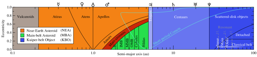
Figure 12: The different classes of SSOs used thorough the article. H stands for Hungarias, and IMB, MMB, and OMB for inner, middle, and outer belt respectively. Comets orbital elements formally overlap with other classes because their classification is based on the presence of a coma at short heliocentric distance.

Class	Semi-major axis (au)		Eccentricity		Perihelion (au)		Aphelion (au)
	min.	max.	min.	max.	min.	max.	min.	max.
NEA	–	–	–	–	–	1.300	–	–
Atira	–	a${}_{\textrm{\earth}}$	–	–	–	–	–	q${}_{\textrm{\earth}}$
Aten	–	a${}_{\textrm{\earth}}$	–	–	–	–	q${}_{\textrm{\earth}}$	–
Apollo	a${}_{\textrm{\earth}}$	4.600	–	–	–	Q${}_{\textrm{\earth}}$	–	–
Amor	a${}_{\textrm{\earth}}$	4.600	–	–	Q${}_{\textrm{\earth}}$	1.300	–	–
MC	1.300	4.600	–	–	1.300	Q${}_{\textrm{\mars}}$	–	–
MBA	Q${}_{\textrm{\mars}}$	4.600	–	–	Q${}_{\textrm{\mars}}$	–	–	–
Hungaria	–	J4:1	–	–	Q${}_{\textrm{\mars}}$	–	–	–
IMB	J4:1	J3:1	–	–	Q${}_{\textrm{\mars}}$	–	–	–
MMB	J3:1	J5:2	–	–	Q${}_{\textrm{\mars}}$	–	–	–
OMB	J5:2	J2:1	–	–	Q${}_{\textrm{\mars}}$	–	–	–
Cybele	J2:1	J5:3	–	–	Q${}_{\textrm{\mars}}$	–	–	–
Hilda	J5:3	4.600	–	–	Q${}_{\textrm{\mars}}$	–	–	–
Trojan	4.600	5.500	–	–	–	–	–	–
Centaur	5.500	a${}_{\textrm{\neptune}}$	–	–	–	–	–	–
KBO	a${}_{\textrm{\neptune}}$	–	–	–	–	–	–	–
SDO	a${}_{\textrm{\neptune}}$	–	–	–	–	37.037	–	–
Detached	a${}_{\textrm{\neptune}}$	–	0.24	–	37.037	–	–	–
ICB	37.037	N2:3	–	0.24	37.037	–	–	–
MCB	N2:3	N1:2	–	0.24	37.037	–	–	–
OCB	N1:2	–	–	0.24	37.037	–	–	–

Table 4: The definition of all the dynamical populations use here, as function of their semi-major axis, eccentricity, perihelion, and aphelion (using the definitions in Carry et al. 2016; Gladman et al. 2008). See Fig. 12 for the distribution of these populations in the semi-major axis - eccentricity orbital element space. The numerical value of the semi-major axes $a$, perihelion $q$, aphelion $Q$, and mean-motion resonances (Indices _i:j) are for the Earth a${}_{\textrm{\earth}}$, q${}_{\textrm{\earth}}$, and Q${}_{\textrm{\earth}}$ at 1.0, 0.983, and 1.017 AU; for Mars Q${}_{\textrm{\mars}}$ at 1.666 AU; for Jupiter J_4:1, J_3:1, J_5:2, J_2:1, and J_5:3 at 2.06, 2.5, 2.87, 3.27, 3.7 AU; and for Neptune a${}_{\textrm{\neptune}}$, N_2:3, and N_1:2 at 30.07, 47.7, and 39.4 AU. The somewhat arbitrary limit of 37.037 AU corresponds to the innermost perihelion accessible to detached KBOs (semi-major axis of N_1:2 and eccentricity of 0.24).

Appendix B Euclid colors and lightcurves of SSOs

Due to the ever changing Sun-SSO-observer geometry and SSO rotating irregular shape, the apparent magnitude of SSOs is constantly changing. Magnitude variations in multi-filter time series are thus a mixture of low frequency geometric evolution, high frequency shape-related variability, and intrinsic surface colors.

The slow geometric evolution can easily be taken into account (Eq. 1), but disentangling the intrinsic surface colors from the shape-related variability is required to build the SED (Section 5) and to obtain a dense lightcurve (Section 8). Often, only the simplistic approach of taking the pair of filters closest in time can be used to determine the color (e.g., Popescu et al. 2016), while hoping the shape-related variability will not affect the color measurements (Fig. 10, Szabó et al. 2004).

The sequence of observation by Euclid in four repeated blocks, each containing all four filters (Fig. 2), however allows a more subtle approach. For any given color, i.e., pair of filter, each filter will be bracketed in time three times by the other filter. The reference magnitudes provided by the bracketing filter allow to estimate the magnitude at the observing time of the other filter. For instance, to determine the (VIS-Y) index, one can use the first two measurements in VIS to estimate what should be the VIS magnitude at the time the Y filter was acquired (by simple linear interpolation for instance). This corrects, although only partially, for the shape-related variability. Hence, any colors will be evaluated six times over an hour, although not entirely independently each time.

The only notable assumption here is that the SED is constant over rotation, i.e., that the surface composition and properties are homogeneous on the surface, which is a soft assumption based on the history of spacecraft rendezvous with asteroids (i.e., Eros, Gaspra, Itokawa, Mathilde, Ida, Šteins, Lutetia, Ceres, with the only exception of the Vesta, see e.g., Veverka et al. 2000; Sierks et al. 2011; Russell et al. 2012).

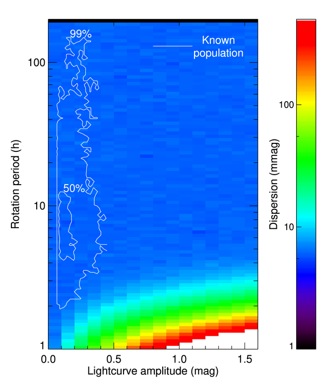
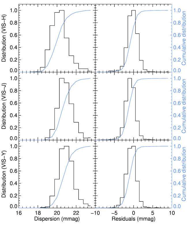
Figure 13: Left: Distribution of the dispersion of color measurement in period-amplitude space. The white contours represent the regions encompassing respectively 50% and 99% of the population with known rotation period and amplitude. Largest uncertainties are found for high-amplitude short-rotation-period lightcurves, outside the typical space sampled by SSOs. Right: Distribution of the dispersion and residuals of color determination in VIS-Y, VIS-J, and VIS-H colors (the remaining colors being a combination of these three). Dispersion is typically at the level of individual measurement uncertainty (here 0.020 magnitude). Residuals are much smaller, close to zero and with dispersion below 0.01 magnitude.

We test this approach by simulating sequences of observation by Euclid. For each of the 371 asteroids of the DeMeo et al. (2009), we simulate 800 lightcurves made of Fourier series of the second order, with random coefficients to produce lightcurve amplitude between 0 and 1.6 magnitude, and random rotation period between 1 and 200 hours. These $\approx$300,000 lightcurves span the observed range of amplitude and period parameter space, estimated from the 5759 entries with a quality code 2 or 3 from the Planetary Data System archive (Fig. 13, Harris et al. 2017). We limit the simulation to second order Fourier series as dense lightcurves for about a thousand asteroids from the Palomar Transient Factory showed that is was sufficient to reproduce most asteroid lightcurves (Polishook et al. 2012; Chang et al. 2014; Waszczak et al. 2015). For each lightcurve, we determine the 4$\times$4 apparent magnitude measurements using the definition of Euclid observing sequence (Fig. 2), the SSO color (from Section 5), and add a random Gaussian noise of 0.02 magnitude.

We then analyze these 4$\times$4 measurements with the method described above. For each SSO and each lightcurve, we determine all the colors (VIS-Y, VIS-J, VIS-H, Y-J, Y-H, J-H) and compare them with the input of the simulation, hereafter the residuals. For each color, we also record the dispersion of estimates.

The accuracy on each colors is found to be at the level of single measurement uncertainty (Fig. 13). This is due to the availability of multiple estimates of each color, improving the resulting signal to noise ratio. The residuals are found very close to zero: offsets below the milli-magnitude (mmag) with a standard deviation below 0.01, i.e., smaller than individual measurement uncertainty (about a factor of five). We repeated the analysis with higher levels of Gaussian noise on individual measurements (0.05 and 0.10 magnitude, the latter corresponding to the expected precision at Euclid limiting magnitude), adding 600,000 simulated lightcurves to the exercise, and found similar results: color uncertainty remains at the level of the uncertainty on individual measurement, and residuals remain close to zero, with a dispersion following the individual measurement uncertainty reduced by a factor of about five. The colors determined with this technique are therefore precise and reliable.

The processing described here is a simple demonstrator that SED can be precisely determined from Euclid multi-filters time series. As a corollary, a single lightcurve of 16 measurements can be reconstructed from the 4$\times$4 measurements. These will be the root of the spectral classification (Section 5) and time-resolved photometry analysis (Section 8). The technique will be further refined for the data processing: we considered here each color, i.e. pair of filters, independently. No attempt for multi-pair analysis was made for this simple demonstration of the technique, while a combined analysis should reduce even further the residuals, i.e., potential biases.